Comparative Study of RNN-Based Deep Learning Models for Practical 6-DOF Ship Motion Prediction

Abstract

Accurate prediction of ship motion is essential for ensuring the safety and efficiency of maritime operations. However, the ship dynamics’ nonlinear, non-stationary, and environment-dependent nature presents significant challenges for reliable short-term forecasting. This study uses a simulated dataset designed to reflect realistic maritime variability to evaluate the performance of recurrent neural network (RNN)-based models—including RNN, LSTM, GRU, and Bi-LSTM—under both single and multi-environment conditions. The analysis examines the effects of input sequence length, downsampling intervals, model complexity, and input dimensionality. Results show that Bi-LSTM consistently outperforms unidirectional architectures, particularly in complex multi-environment scenarios. In single-environment settings, the prediction horizon exceeded 40 s, while it decreased to around 20 s under more variable conditions, reflecting generalization challenges. Multi-degree-of-freedom (DOF) inputs enhanced performance by capturing the coupled nature of ship dynamics, whereas incorporating wave height data yielded inconsistent results. A sequence length of 200 timesteps and a downsampling interval of 5 effectively balanced motion feature preservation with high-frequency noise reduction. Increasing model size improved accuracy up to 256 hidden units and 10 layers, beyond which performance gains diminished. Additionally, Peak Matching was introduced as a complementary metric to MSE, emphasizing the importance of accurately predicting motion extrema for practical maritime applications.

1. Introduction

Accurate prediction of wave-induced ship motions has long been recognized as a fundamental challenge in marine engineering and autonomous navigation system development [1,2,3]. Ships exhibit complex six degrees-of-freedom (6-DOF: surge, sway, heave, roll, pitch, yaw) dynamics under varying sea conditions and operational speeds [4]. Particularly in challenging sea conditions with high wave variability, precise prediction of dynamic responses to wave excitation plays a crucial role in ensuring autonomous system stability and expanding operational envelopes [5]. Consequently, extensive research has been directed toward developing methods for predicting short-term ship motion responses faster than in real time.

Early research primarily focused on numerical analysis-based models such as Kalman filters [6], followed by the adoption of statistical time series models based on Auto-Regression (AR) and Auto-Correlation Function (ACF) for predicting roll, pitch, and heave motions [7,8]. While these models offer advantages in terms of simplicity and interpretability, they face significant limitations in adequately capturing the highly nonlinear characteristics of ship motions [9]. Recent work has also validated Kalman filtering for ship-movement prediction using operational AIS-type inputs, underscoring the practicality of classical estimators in maritime settings [10]. Quaternion-based Kalman filtering has also been explored for distributed orientation estimation [11]. Such methods are primarily suited for sensor fusion and attitude tracking. Traditional AR models depend on predefined parameters and exhibit poor adaptability to diverse operational scenarios, particularly when dealing with non-stationary ship motion time series [12]. Furthermore, ACF-based methods suffer from significant lag time errors in instantaneous sample calculations, limiting their real-time prediction capabilities [13].

In recent years, deep learning-based time series prediction models have been increasingly adopted to address these limitations [14,15]. RNN-based models, particularly LSTM and GRU architectures, have demonstrated superior capability in learning complex ship dynamics and promise for full 6-DOF prediction [16,17]. For maritime trajectory prediction using AIS data, recurrent models (LSTM/GRU) outperform classical baselines when combined with rigorous preprocessing and spatiotemporal handling [18]. Various approaches have been explored to enhance prediction accuracy and generalization performance, including encoder–decoder structures with attention mechanisms [19], input vector optimization, wavelet-based multi-scale processing [20], and hybrid architectures incorporating CNN components [21]. Beyond maritime applications, physics-guided GNNs and transformers improve forecasting by combining topology, signals, and temporal embeddings [22,23], suggesting that such designs could also advance maritime motion prediction.

Recent studies have incorporated advanced optimization strategies to improve model performance. Particle Swarm Optimization (PSO) algorithms have been successfully applied to optimize bidirectional LSTM networks for ship motion attitude prediction, demonstrating enhanced accuracy compared to conventional approaches [24]. Similarly, Binary System Optimization (BSO) algorithms have optimized complex hybrid architectures combining Temporal Convolutional Networks with BiGRU and attention mechanisms [25]. These optimization strategies have shown meaningful progress in real-time capability and prediction accuracy through systematic hyperparameter tuning and architectural refinement. Beyond pure deep models, hybrid approaches combining physics and learning are increasingly applied in transport and marine domains [26,27]. For ship motions, comparisons of physics-informed and data-driven models reveal an accuracy–interpretability trade-off, underscoring the need for clear baselines [28,29].

However, most studies remain limited by their reliance on data collected under specific ocean conditions or focus on partial DOF [30]. Significant challenges persist in simultaneously addressing the complexity and diversity of actual operational conditions while achieving precise predictions for all 6-DOF. Furthermore, overfitting issues, where models become excessively adapted to training data and exhibit degraded performance in test environments, continue to be reported [8,31]. Neural network models for ship motion prediction face particular challenges in generalization, requiring careful validation strategies to prevent overfitting while maintaining prediction accuracy across varying maritime conditions [32].

The present study systematically investigates the prediction performance of four representative RNN-based architectures (RNN, LSTM, GRU, Bi-LSTM) under single- and multi-sea-state environments (Section 3, Section 4 and Section 5). It quantifies the effects of input sequence length, downsampling interval, model scale, and input dimensionality. In addition, using both standard error metrics (MSE/MAE) and peak-related evaluation indicators enables the formulation of practical design guidelines for real-world implementation. Given the growing interest and adoption of deep learning models in maritime applications, there is a critical need for comprehensive comparative studies that can guide researchers and engineers in selecting appropriate architectures.

The contributions of this paper can be summarized as follows:

• Unified baseline for 6-DOF prediction. Four representative RNN-based models were systematically compared under consistent experimental conditions, establishing a practical baseline for ship motion prediction across maritime environments.
• Basic RNN model design insights. Practical guidelines were designed using basic PyTorch libraries (version 2.8.0) on sequence length, downsampling strategy, input dimensionality, and model capacity, highlighting conditions under which RNN-based models can achieve stable and reliable performance.
• Safety-relevant evaluation. Peak Matching and the Overestimation Ratio were proposed as complementary evaluation metrics to traditional error measures, emphasizing the importance of extrema prediction for safety-critical maritime operations.

2. Related Works

Table 1. Summary of related studies, including data acquisition methods, degrees of freedom considered in the time series, and inclusion of external forces.

Paper	Base Methodology	Data Type	Motion	Wave	Other Factors
Yumori (1981) [2]	AR	Real Data	1DOF (Heave)	O	O
Zhao et al. (2004) [3]	MCA	Simulation	6DOF	O	X
Takami et al. (2021) [7]	ACF	Real	2DOF (Heave, Roll)	O	O
Li et al. (2017) [9]	Neural Network	Real	2DOF (Roll, Pitch)	X	O
Zhang et al. (2023) [14]	Transformer	Real	6DOF	O	O
Duan et al. (2015) [31]	AR	Simulation	2DOF (Pitch, Heave)	O	-
Nielsen & Jensen (2017) [32]	ACF	Real	3DOF (Roll, Pitch, Heave)	O	X
Nielsen et al. (2018) [33]	ACF	Simulation	3DOF (Heave, Roll, Pitch)	O	X
Jiang et al. (2020) [34]	AR	Model test	2DOF (Pitch, Heave (Roll))	X	X
Zhang et al. (2023) [35]	Kalman Filter	Simulation	3DOF (Surge, Sway, Yaw)	X	O
Yin et al. (2013) [36]	Neural Network	Real	1DOF (Roll)	X	X
Zhang & Liu (2014) [37]	Neural Network	Real	2DOF (Roll, Yaw)	O	O
Li et al. (2017) [38]	Neural Network	Real	1DOF (Roll)	X	O
Skulstad et al. (2021) [39]	Neural Network	Real	3DOF (Surge, Sway, Yaw)	X	O
Silva & Maki (2022) [40]	LSTM	Simulation	6DOF	O	X
Lee et al. (2023) [41]	LSTM	Simulation	2DOF (Heave, Pitch)	O	X
Tian & Song (2023) [42]	LSTM	Simulation	1DOF (Roll)	O	O
Lee et al. (2023) [43]	LSTM	Simulation	2DOF (Heave, Pitch)	O	X
D’Agostino et al. (2022) [44]	RNN, LSTM, GRU	Simulation	6-DOF	O	O
Liu et al. (2020) [45]	LSTM	Simulation	2DOF (Pitch, Heave)	O	X
Zhou et al. (2023) [46]	GRU	Real	1DOF (Roll)	O	X
Zhang et al. (2021) [47]	LSTM	Simulation	3DOF (Roll, Pitch Heave)	O	X
Gao et al. (2023) [48]	RNN	Simulation	2DOF (Roll, Pitch)	O	O
Gong et al. (2025) [49]	LSTM	Simulation	6DOF	O	O
Xu & Yin (2024) [50]	SVR	Real	1DOF (Roll)	O	X
Mak & Düz (2019) [51]	CNN-RNN	Real	6DOF	O	O
Shi et al. (2025) [52]	CNN-Transformer	Simulation, Real	1DOF (Heave)	O	X
Zhang et al. (2023) [53]	TCN-Attention	Real	3DOF (Roll, Pitch, Heave)	O	X
Zhang et al. (2024) [54]	CNN-RNN	Real	6DOF	O	O
Lee et al. (2024) [55]	CNN, RNN	Simulation	3DOF (Heave, Roll, Pitch)	O	X

presents a comprehensive overview of existing studies organized according to several key criteria: prediction methodologies employed, data types (simulation or measured data), DOF of ship motions predicted, utilization of wave information as input variables, and inclusion of external environmental variables such as wind speed and ship state variables, including vessel speed, position, and hull length. This systematic categorization enables a comparative analysis of the scope of problems addressed, the complexity of input configurations, and differences in modeling approaches across various studies. Specifically, the “Base Methodology” column summarizes the fundamental technical approach adopted in each study. The “Data Type” classification distinguishes between simulation data obtained from numerical or CFD analysis, model test data collected from physical scale experiments, and real-world data measured from operating vessels. The “Motion” category specifies which of the six degrees of freedom (DOF) of ship motion were considered in the analysis. The “Wave” column indicates whether wave information was included as an external forcing variable. At the same time, other environmental and operational inputs such as wind speed, vessel speed, and ship dimensions are listed under “Other Factors”. This detailed categorization provides insights into how input variables and environmental conditions were structured and addressed in previous research.

With the advent of machine learning techniques, statistical time series models based on Auto Regression (AR) and Auto-Correlation Function (ACF) have gained widespread adoption in ship motion prediction. Yumori [2] pioneered AR and Moving Average methods to achieve up to 10 s ahead predictions for the heave motion. Subsequently, researchers expanded the prediction scope to encompass up to three degrees of freedom, including roll, pitch, and heave, using AR and ACF-based models [7,31,32,33]. Jiang et al. [34] demonstrated that prediction performance varies with wave spectrum characteristics and hull dimensions, indicating the sensitivity of AR model performance to environmental conditions. The traditional Kalman filter approach remains valid and effective. Zhang et al. [35] proposed a real-time collision avoidance decision-making system integrated with autonomous navigation control, utilizing 3-DOF MMG models combined with numerical analysis and Kalman filter-based trajectory prediction. While these statistical models offer relatively efficient and straightforward short-term predictions without requiring wave information, they exhibit limitations in adapting to sea state variations, capturing nonlinear ship motion characteristics, and providing long-term predictions. Furthermore, the requirement for offline learning to predefine model parameters restricts their flexibility in responding to diverse operational scenarios.

Deep learning-based time series prediction models have been actively introduced to overcome these limitations. Yin et al. [36] demonstrated the feasibility of roll prediction using neural network-based models. At the same time, Zhang and Liu [37] employed Time-delay Wavelet Neural Networks to incorporate dynamic system characteristics and enhance generalization capabilities. Li et al. [38] partly showed the superiority of neural network-based predictions over time series analysis-based AR models. Skulstad et al. [39] proposed a Co-operative Hybrid Model combining physics-based dynamic models with neural networks, presenting an approach to compensate for prediction errors arising from mismatches and unmeasured external forces. However, these studies predominantly focused on limited degrees of freedom, such as roll and pitch, or were trained under specific sea state conditions, thus exhibiting limitations in generalization performance across diverse operational conditions.

Recent developments have witnessed the application of various time series prediction techniques to ship motion forecasting, with particular emphasis on RNN-based deep learning models. Silva and Maki [40] proposed an LSTM (Long Short-Term Memory) model utilizing wave height information as input to predict all six degrees of freedom. Lee et al. [41] incorporated wave elevation data into the input of an LSTM model to obtain time series of ship motion responses, specifically heave and pitch, and linear motion response functions. Tian et al. [42] demonstrated that incorporating wave elevation data as an LSTM input significantly improves the accuracy and provides adequate lead time for roll motion prediction. A modification of the LSTM model using wave elevation as an input have been introduced, enabling more accurate prediction of ship motions [43]. Based on CFD-generated wave and motion data, their study showed that multi-point wave elevation inputs enhance model robustness and stability by increasing data richness and depth. D’Agostino et al. [44] conducted a comparative multi-DOF motion prediction performance analysis using Encoder–Decoder architectures based on RNN, LSTM, and GRU. While these approaches demonstrated generally favorable prediction results, relatively lower prediction accuracy was observed for specific degrees of freedom (e.g., sway), and higher errors in test data compared to training data indicated tendencies toward overfitting. These findings align with observations by Li et al. [38], who compared the advantages and disadvantages of various prediction models and highlighted the vulnerability of neural networks to overfitting. Such results underscore the necessity for careful consideration to avoid overfitting to specific marine conditions. This study shares this perspective and aims to secure generalization performance without overfitting through data-driven learning, reflecting the complexity and diverse conditions of marine environments.

Many different approaches have been explored to enhance prediction accuracy in ship motion forecasting. Liu et al. [45] improved LSTM learning efficiency through input vector space optimization, while Zhou et al. [46] combined GRU with signal decomposition techniques, utilizing Binary System Optimization (BSO) for VMD parameter tuning. Wavelet-based methods have been actively employed to address the nonlinear and non-stationary nature of ship motion data. Zhang et al. [47], Gao et al. [48], and Gong et al. [49] introduced wavelet-transformed multi-frequency features into models incorporating attention mechanisms, residual RNNs, and PCA-enhanced LSTM architectures, respectively, to improve accuracy and generalization. Furthermore, Xu and Yin [50] proposed a hybrid ship roll prediction scheme combining TVF-EMD and support vector regression, optimized using an improved black widow algorithm, which achieved superior performance over conventional decomposition-based methods using real sea data.

Additionally, attempts combining CNN and Transformer architectures have increased. Mak et al. [51] utilized CNN and RNN to estimate relative wave directions from ship motion time series. Shi et al. [52] developed a multi-step heave prediction model for active compensation control by combining attention-based multi-scale CNN with Transformer encoders. Zhang et al. [53] proposed a ship motion prediction model that integrates an Improved Whale Optimization Algorithm (IWOA), Temporal Convolutional Networks (TCN), and an attention mechanism, effectively enhancing prediction accuracy by extracting long-term temporal features, emphasizing critical components through attention weighting, and optimizing hyperparameters via IWOA. Zhang et al. [14] improved the 6-DOF prediction performance of Transformer-based models by integrating various real-world data sources, including AIS, bathymetry, and nowcast data. Zhang et al. [54] achieved high prediction accuracy through a hybrid spatial-temporal model combining CNN-MRNN with IADPSO. Instead of relying solely on wave elevation time history data at a fixed location obtained from simulations, it is possible to develop an RNN-based prediction model that utilizes two-dimensional wave information acquired through real-time sensing technologies such as cameras or radar data [55].

3. Neural Networks

While traditional statistical models have demonstrated reasonable performance in short-term predictions or single-degree-of-freedom motion forecasting, their limitations become evident in real-world scenarios requiring simultaneous consideration of complex marine environments and 6-DOF ship motions. Deep learning-based time series prediction models have been actively introduced to address these challenges in recent years, with particular attention given to Recurrent Neural Network (RNN) architectures. Since this study aims to predict time series of future ship motions from a specific point in time, RNN-based artificial neural network models are most closely aligned with the physical characteristics of our research objectives. Therefore, we examine four representative recurrent neural network models, with their schematic representations illustrated in Figure 1. This section briefly introduces the structural characteristics and operational principles of RNN, Long Short-Term Memory (LSTM), Gated Recurrent Unit (GRU), and Bidirectional LSTM (Bi-LSTM).

3.1. Recurrent Neural Network (RNN)

RNN is an architecture designed to model temporal dependencies in time series data by updating the current hidden state by considering both the current input and previous hidden state [56]. This structure effectively captures the sequential nature of input sequences and is expressed by the following equation:

$$h_t=\tanh \left(W_{xh}{x}_t+W_{hh}{h}_{t-1}+b_h\right)$$

(1)

where $h_t$ represents the hidden state at time $t$, $x_t$ is the input at time $t$, $y_t$ is the output at time $t$, $W_{hh}$, $W_{xh}$, and $W_{hy}$ are weight matrices, and $b_h$ and $b_y$ are bias vectors. At each time step, the hidden state is updated using a nonlinear activation function such as hyperbolic tangent $\left(tanh\right)$, incorporating both the current input and previous hidden state. However, conventional RNN structures suffer from the vanishing gradient problem, leading to information loss as sequences become longer, which limits their ability to capture long-term dependencies [57].

3.2. Long Short-Term Memory (LSTM)

LSTM was designed to address the long-term dependency problem of RNNs by introducing a cell state and three gates to control information flow [58]. The following equations define the LSTM operations:

$$f_t=\sigma \left(W_f\left[h_{t-1},x_t\right]+b_f\right)$$

(2)

$$i_t=\sigma \left(W_i\left[h_{t-1},x_t\right]+b_i\right)$$

(3)

$$\widetilde{C_t}=\mathit{tanh}\left(W_C\left[h_{t-1},x_t\right]+b_C\right)$$

(4)

$$C_t=f_t\cdot C_{t-1}+i_t\cdot \widetilde{C_t}$$

(5)

$$o_t=\sigma \left(W_o\left[h_{t-1},x_t\right]+b_o\right)$$

(6)

$$h_t=o_t\cdot \mathit{tanh}\left(C_t\right)$$

(7)

where $\sigma$ denotes the sigmoid activation function, $\cdot$ represents element-wise multiplication, and $\left[h_{t-1},x_t\right]$ indicates concatenation of vectors.

The Forget Gate ($f_t$) selectively determines which information from the previous cell state to retain or discard. Values close to 0 indicate information to be forgotten, while values close to 1 indicate information to be retained. The Input Gate ($i_t$) determines which parts of new information should be added to the cell state based on the current input and previous hidden state. The candidate cell state ($\widetilde{C_t}$) represents potential new information generated from the current input that could be added to the cell state. The new cell state ($C_t$) is updated by combining the selected portions of the previous cell state (through the Forget Gate) with the chosen new candidate information (through the Input Gate). This mechanism enables LSTM to integrate new information while effectively maintaining important past information. Output Gate ($o_t$) determines which information from the cell state should be sent to the output, with values close to 0 indicating minimal contribution to the output. Finally, the hidden state ($h_t$) is calculated by multiplying the output gate values with the hyperbolic tangent of the cell state. This architecture allows LSTM to separately process information to be output at each time step and information to be maintained internally, enabling stable learning and prediction without information loss even for long sequence predictions.

3.3. Gated Recurrent Unit (GRU)

GRU represents a simplified version of LSTM that merges the cell and hidden states while utilizing only two gates [59]. The following equations describe the GRU operations:

$$z_t=\sigma \left(W_z\left[h_{t-1},x_t\right]+b_z\right)$$

(8)

$$r_t=\sigma \left(W_r\left[h_{t-1},x_t\right]+b_r\right)$$

(9)

$$h{̃}_t=tanh\left(W_h\left[r_t\cdot h_{t-1},x_t\right]+b_h\right)$$

(10)

$$h_t=\left(1-z_t\right)\cdot h_{t-1}+z_t\cdot h{̃}_t$$

(11)

The Update Gate ($z_t$) determines how much past information to retain, while the Reset Gate ($r_t$) determines how much past information to forget. The final hidden state is updated based on the Update Gate and candidate hidden state. Due to its simpler structure, GRU offers faster computational speed while providing prediction performance comparable to LSTM, making it efficient for long sequence prediction problems.

3.4. Bidirectional LSTM (Bi-LSTM)

A bidirectional structure for RNNs was first proposed by M. Schuster and K. K. Paliwal (1997) [60], enabling the model to incorporate both forward and backward temporal dependencies. This structure was later combined with the Long Short-Term Memory (LSTM) architecture, resulting in the widely adopted Bidirectional LSTM (Bi-LSTM). Equations (12)–(14) illustrate the operational mechanism of Bi-LSTM.

$${\overrightarrow{h}}_t=\mathrm{LST}{\mathrm{M}}_{\mathrm{fwd}}\left(x_t\right)$$

(12)

$${\overleftarrow{h}}_t=\mathrm{LST}{\mathrm{M}}_{\mathrm{bwd}}\left(x_t\right)$$

(13)

$$h_t=[{\overrightarrow{h}}_t;{\overleftarrow{h}}_t]$$

(14)

where ${\overrightarrow{h}}_t$ and ${\overleftarrow{h}}_t$ represent the forward and backward hidden states, respectively, and [;] denotes concatenation.

While the forward LSTM processes the input sequence in chronological order, the backward LSTM processes the same sequence in reverse. The hidden states from both directions are combined to form the final representation. Because Bi-LSTM captures contextual information in both temporal directions, it has been shown to outperform unidirectional LSTM models in time series forecasting tasks [61]. Furthermore, the backward pass of Bi-LSTM was implemented without feeding future measurements beyond the given input window. The same input sequence was processed forward and reverse, ensuring a fair comparison with unidirectional models.

4. Materials and Methods

This section describes the data, preprocessing procedures, model architectures, and training and evaluation methods used to construct time series prediction models applicable to marine operational environments. Figure 2 schematically illustrates the overall experimental process, depicting the procedure for predicting future ship motions by training RNN-based models (RNN, LSTM, GRU, Bi-LSTM) using ship motion and wave data. The experiments were conducted stepwise, deriving the optimal model in a single environment, then extending its application to nine diverse marine environments. This approach systematically verified prediction performance, generalization capability, and adaptability to environmental changes in single and multiple environments.

Additionally, model performance was compared and analyzed based on input data configuration (single DOF vs. 6-DOF) and wave time series data inclusion to examine the impact of input variable settings on prediction performance. The main experimental configurations are as follows:

To evaluate the influence of input variable configurations on prediction performance, model comparisons were conducted concerning input motion complexity (single DOF vs. 6-DOF) and the inclusion of wave time series data—the experimental framework comprised four major configurations. First, to assess the effect of environmental diversity on model generalization, models trained on data from a single environment were compared to those trained on integrated data from nine different environments. Second, the impact of input motion degrees of freedom was examined by comparing models using single-DOF input data with those utilizing full 6-DOF input, thereby evaluating the influence of variable complexity. Third, the contribution of wave information to prediction accuracy was analyzed by including or excluding wave data in the input variables. Fourth, the effect of input sequence length was investigated to determine its influence on predictive performance and the maximum horizon of accurate forecasting. This led to the identification of optimal sequence lengths for practical implementation. Lastly, the impact of down-sampling input variations on prediction performance and computational efficiency was analyzed, and an appropriate sampling interval was identified to balance information retention and model accuracy.

4.1. Experimental Setup

4.1.1. Dataset

The wave-induced motions of a ship were simulated using a time-domain approach grounded in the impulse response function (IRF) methodology, as introduced by Cummins (1962) [62]. The model accounts for 6-DOF motions—namely surge ${\xi }_1$, sway ${\xi }_2$, heave ${\xi }_3$, roll ${\xi }_4$, pitch ${\xi }_5$, and yaw ${\xi }_6$ at the vessel’s forward speed. Each regular wave component is characterized by its amplitude $A_n$, frequency ${\omega }_n$, propagation direction (or heading angle) ${\chi }_n$, and phase ${\epsilon }_n$ for the wave excitation.

The governing equations of motion can be expressed as follows:

$$\left(M_{jk}+M_{jk}^{\infty }\right){\ddot{\xi }}_k+{\int }_{-\infty }^t{R}_{jk}\left(t-\tau \right){\dot{\xi }}_k\left(\tau \right)d\tau +C_{kj}^R{\xi }_k=F_{r,j}+F_{F.K,j}+F_{d,j}$$

(15)

Here, $M_{jk}$ and $M_{jk}^{\mathrm{\infty }}$ represent the mass matrix and the added mass matrix at infinite frequency, respectively. The term $C_{kj}^R$ corresponds to the restoring coefficient modified by the forward motion of the vessel [63]. The memory effect of past motions is captured by the retardation function $R_{jk}$, which is derived from the frequency-dependent added mass $A_{jk}\left(\omega \right)$ and damping coefficient $B_{jk}\left(\omega \right)$ via Fourier transformation.

$$R_{jk}\left(t\right)={\displaystyle \frac{2}{\pi }}{\int }_0^{\infty }{B}_{jk}\left(\omega \right)cos\left(\omega t\right)d\omega$$

(16)

$$M_{jk}^{\infty }-{\displaystyle \frac{C_{kj}^R}{{\omega }^2}}=A_{jk}\left(\omega \right)+{\displaystyle \frac{1}{\omega }}{\int }_0^{\infty }{R}_{jk}\left(\tau \right)sin\left(\omega \tau \right)d\tau$$

(17)

The hydrodynamic coefficients required to calculate the retardation function were obtained from two-dimensional (2D) strip theory computations [64]. In this simulation framework, hydrostatic restoring forces $F_{r,j}$ and Froude–Krylov forces $F_{F.K,j}$ were computed directly from the instantaneous wetted surface of the hull, accounting for both the incident wave profile and the resulting ship motions in the time domain. Additionally, the wave diffraction forces $F_{d,j}$ were evaluated using transfer functions derived from the same 2D strip theory. This hybrid approach allows for partial incorporation of the nonlinearities arising from complex hull geometries, thereby constituting a weakly nonlinear simulation framework.

To develop the training dataset for the neural network models, the KRISO Container Ship (KCS) was chosen as the representative vessel, with its principal particulars provided in

Table 2. KCS model details.

	Values
L [m]	230
B [m]	32.2
T [m]	10.8
∇ [m]	52,030
$x_G$ [m], fwd+	−1.480
$C_b$	0.651
$k_{yy}$/L	0.250

. Assuming operation at the design cruising speed, simulations were carried out under multiple sea conditions, as detailed in

Table 3. Database description.

	Values
$\mathrm{Mean}\mathrm{period},T_{mean}$ [s]	7.5	9.5	11.5	7.5	9.5	11.5	7.5	9.5	11.5
$\mathrm{Propagation}\mathrm{direction},\chi$ [deg]	90	90	90	135	135	135	180	180	180
$\mathrm{Significant}\mathrm{height},H_S$ [m]	3.5
Simulation time [s]	10,000 for each condition
$\mathrm{Time}\mathrm{step},dt$ [s]	0.01

, by combining various sea states with different wave heading angles. A long-crested irregular wave field was generated by decomposing the ITTC wave spectrum into 100 sinusoidal components with random phase superposition to mimic natural irregularity. For each condition, time-series data of the 6-DOF ship motions were produced over 10,000 s with a sampling interval of 0.01 s, resulting in 90,000 s of simulation and about 9 million data points in total. This dataset was balanced across all environmental conditions to ensure fair model training. To capture the nonlinear dependence of ship responses on sea-state severity, a total of eighteen sea states with different significant wave heights and mean periods were considered, restricted to long-crested irregular head seas. The motion databases were generated through weakly nonlinear IRF-based simulations. Independent test sets were configured for each operating scenario to evaluate the generalization performance of the models.

4.1.2. Data Preprocessing

Gaussian normalization was applied to remove scale differences between environments to improve model training stability and convergence speed [39]. This prevented excessive dependence on value ranges of specific environments and induced uniform learning effects across all environments.

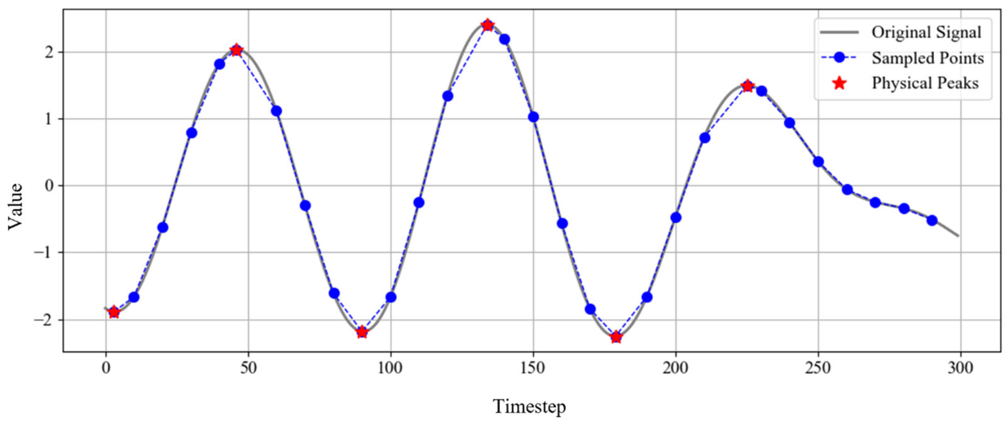
Considering the vulnerability of RNN-based models to long-term dependencies, data within the same time range was downsampled at regular intervals. In addition to the original high-resolution time series, experiments utilized data sampled at n = {2, 5, 10} intervals. However, simple downsampling can omit physically significant peaks (local maxima/minima) in the time series. A peak-preserving correction method was applied to address this. When no actual peak exists within a downsampling interval, the sampled value closest to the actual peak within that interval is designated as a substitute peak value. This approach maintains key dynamic characteristics while reducing resolution, enabling effective prediction even in downsampled environments.

Figure 3 visualizes an example under a downsampling interval n = 10, where the gray line represents the original signal, blue dots indicate sampled points, and red stars mark corrected actual peak points. This correction process ensures the validity of data configuration by preventing the omission of critical physical events.

4.2. Model Architecture and Training

4.2.1. Model Architecture

Four recurrent neural network architectures—RNN, LSTM, GRU, and Bi-LSTM—were compared for time series prediction. Experiments were conducted with three input variable configurations: (1) single DOF (heave), (2) full 6-DOF, and (3) 6-DOF plus wave height information (see Figure 1). All input variables were normalized through Gaussian normalization to remove scale differences between various environments and ensure training stability.

Model outputs were configured as 6-DOF motion predictions for future intervals following the input sequence. All models were trained on identical input sequence lengths and datasets to ensure fair performance comparison between architectures. The intended scope of the present study is primarily offline or near-real-time prediction scenarios where a short delay is acceptable (e.g., decision support, risk assessment, or planning). Unidirectional models would be more appropriate for strictly real-time control applications, but Bi-LSTM was included here to establish comparative baselines and explore their potential for operational analysis.

4.2.2. Training

All experiments were conducted on a workstation with an NVIDIA GeForce RTX 3090 GPU. On average, training time per epoch was approximately 1.7 s (RNN), 2.0 s (LSTM), 1.9 s (GRU), and 2.6 s (Bi-LSTM), confirming that training was computationally feasible under this setting.

In addition, the core hyperparameters—including hidden units, number of layers, batch size, and input sequence configurations—were kept consistent across experiments. These settings are summarized in

Table 4. Summary of the baseline hyperparameter settings for all models.

Model	Sequence Length	Downsampling	Hidden Units	Layers	Batch Size	Learning Rate (Initial)	Loss Function
RNN	{50, 100, 200, 300, 400, 500}	{1, 2, 5, 10}	64	2~10	64~	0.01 → 1 × 10−6	MSE
LSTM	{50, 100, 200, 300, 400, 500}	{1, 2, 5, 10}	64	2~10	64~	0.01 → 1 × 10−6	MSE
GRU	{50, 100, 200, 300, 400, 500}	{1, 2, 5, 10}	64	2~10	64~	0.01 → 1 × 10−6	MSE
Bi-LSTM	{50, 100, 200, 300, 400, 500}	{1, 2, 5, 10}	64	2~20	64~	0.01 → 1 × 10−6	MSE

to ensure reproducibility and provide a clear reference for model configurations. The number of layers was set to a minimum of 2 and increased stepwise (up to 20 for Bi-LSTM) to evaluate performance scalability depending on problem complexity. Similarly, the batch size was set to 64 as the most stable configuration, with additional tests conducted using larger batch sizes for sensitivity analysis.

Mean Squared Error (MSE) was used as the loss function with Adam optimizer for model training. Early stopping was implemented to prevent overfitting and enhance generalization performance across diverse marine environments. This technique terminates training when validation loss shows no improvement for a specified number of epochs, selecting the optimal weights up to that point as the final model.

The initial learning rate was set to 0.01, with adaptive learning rate scheduling applied to reduce the rate by a factor of 0.5 when validation performance plateaued for a specific period. The minimum learning rate was 1 × 10⁻⁶ to ensure training stability and convergence performance.

All models were trained under identical conditions: same data configuration, Gaussian normalization-based standardization, input sequence length, and downsampling intervals n = {1, 2, 5, 10}. This experimental design enabled fair and consistent performance comparison between architectures. Performance evaluation was comprehensively conducted using quantitative metrics, including MSE, MAE, and peak matching-based indicators.

4.3. Evaluation: Metrics and Peak Matching Algorithm

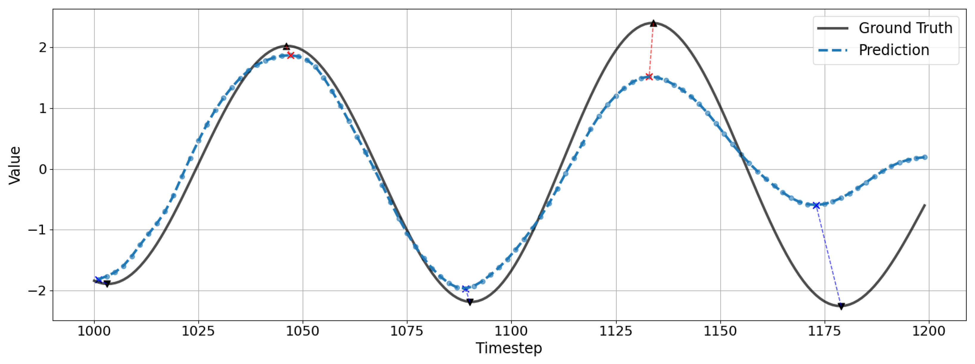
Model performance evaluation was conducted using MSE (Mean Squared Error) across the entire test data range and prediction accuracy at peak (local maxima/minima) intervals, which is crucial in marine engineering for ship motion time series. Since peak regions are directly related to ship control and safety, quantitative analysis beyond general average errors is necessary. To evaluate how accurately the predicted time series captures the peak values of the ground truth data, it is essential to compare the magnitudes of corresponding peaks. However, due to phase shifts between the predicted and actual time series, a dedicated algorithm is required to identify the matching peaks for comparison correctly. An example of this discrepancy is presented in Figure 4.

To address this challenge, we developed a Peak Matching algorithm to quantitatively evaluate the correspondence between predicted and actual time series peaks. This algorithm identifies the most closely matching predicted peak candidates to actual peaks within specified intervals, operating under the following constraints:

• Step 1: Peak Candidate Extraction—Extract peak candidate points from the predicted time series at intervals of n timesteps.
• Step 2: Peak Matching—Match peak candidates within ±n timesteps of actual peaks in the ground truth data to their corresponding local maxima/minima.
• Step 3: Uniqueness Constraint—Ensure no duplicate matching occurs for the same actual peak, maintaining a minimum separation of n timesteps between matched peaks.
• Step 4: Temporal Ordering Constraint—Enforce sequential matching by selecting only peaks that occur after previously matched peaks, preserving temporal causality.

This algorithm was specifically designed to prevent coincidental matching of physically meaningless predicted values that may occur during simple MSE-based loss minimization processes. Instead, it enables focused performance analysis at genuinely significant points in the time series. This approach provides a more reliable evaluation of physically important peak prediction performance that conventional average error metrics cannot adequately capture.

Formally, the Peak Matching score is defined as:

$$PM={\displaystyle \frac{1}{N_m}}\sum _{i=1}^{N_m}1\left(|\widehat{p_i}-p_i|\le ϵ\right)$$

(18)

where $p_i$ denotes the actual peak value, $\widehat{p_i}$ represents the corresponding predicted peak value, ϵ is the allowable error tolerance, and $N_m$ is the total number of successfully matched peaks. The indicator function 1(⋅) equals 1 if the condition is satisfied and 0 otherwise. The tolerance ϵ was determined from the distribution of validation peak errors (e.g., percentile- or MAD/IQR-based thresholds), ensuring robustness against heavy-tailed noise and avoiding arbitrary hand-tuning. This formulation quantifies the proportion of correctly matched peaks within a predefined tolerance, complementing conventional error metrics (MSE, MAE) by focusing on local extrema that are critical in safety-sensitive ship motion prediction.

Furthermore, in marine environments, overestimating predicted values may be more advantageous than underestimating from a vessel control perspective, as it allows for more conservative operational decisions. Accordingly, we incorporated the Overestimated Peak Ratio as an additional analytical metric, quantifying the proportion of peaks where predicted values exceed actual values. This metric provides crucial interpretive information regarding model prediction tendencies and safety assurance aspects, contributing to a comprehensive understanding of model behavior in practical applications.

5. Results

5.1. Single Environment Evaluation

The time series prediction performance was compared and analyzed in a relatively less challenging single marine environment. The comparison models included RNN, LSTM, GRU, and Bi-LSTM, with all experiments conducted under unified conditions of 64 hidden nodes and two layers.

5.1.1. Effect of Trained Sequence Length and Down-Sampling

The analysis examined how prediction performance varies with input sequence length (SL) and downsampling interval (n). Sequence lengths were set as 50, 100, 200, 300, 400, and 500. The downsampling intervals (n) were set as n = {1, 2, 5, 10}, with all models trained using identical architectures.

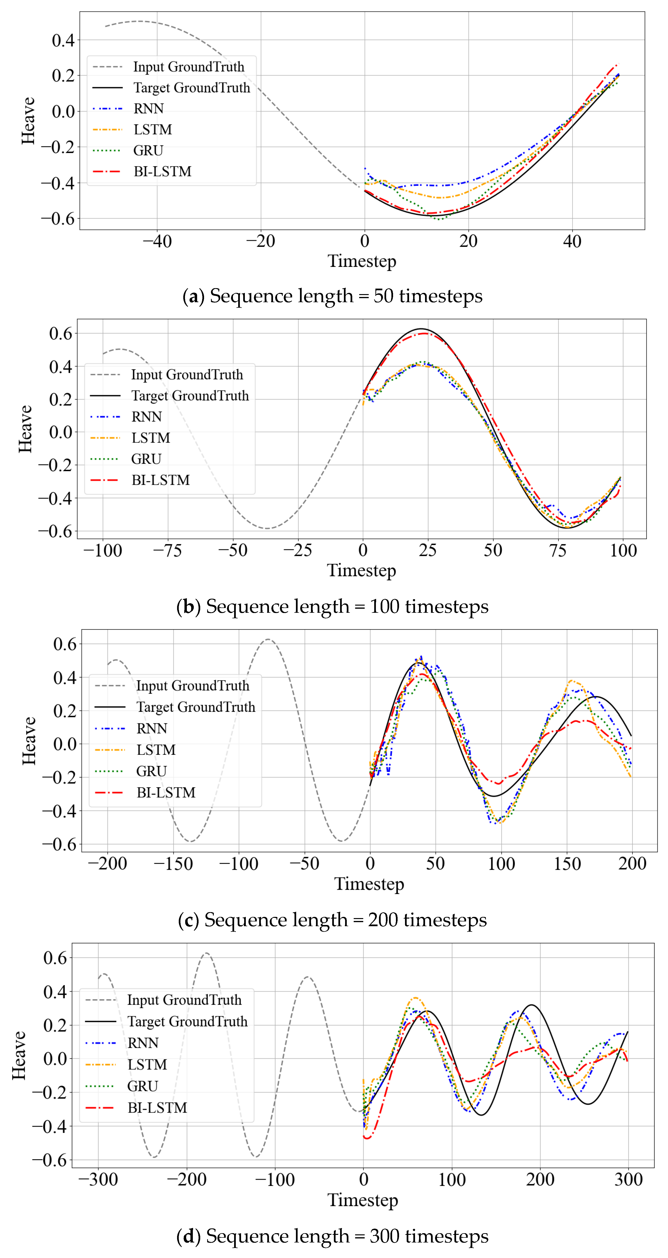
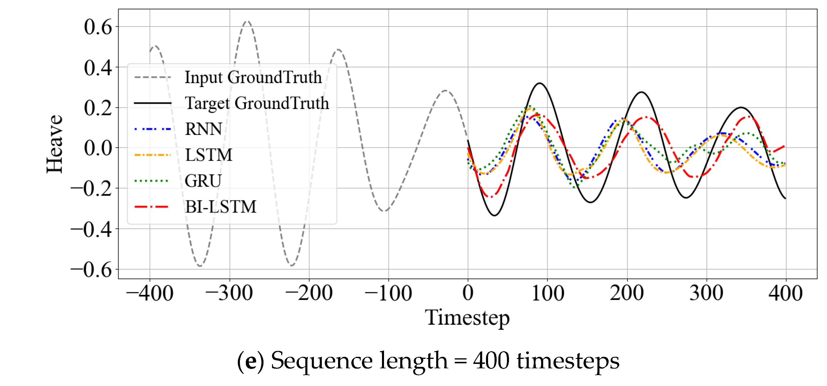
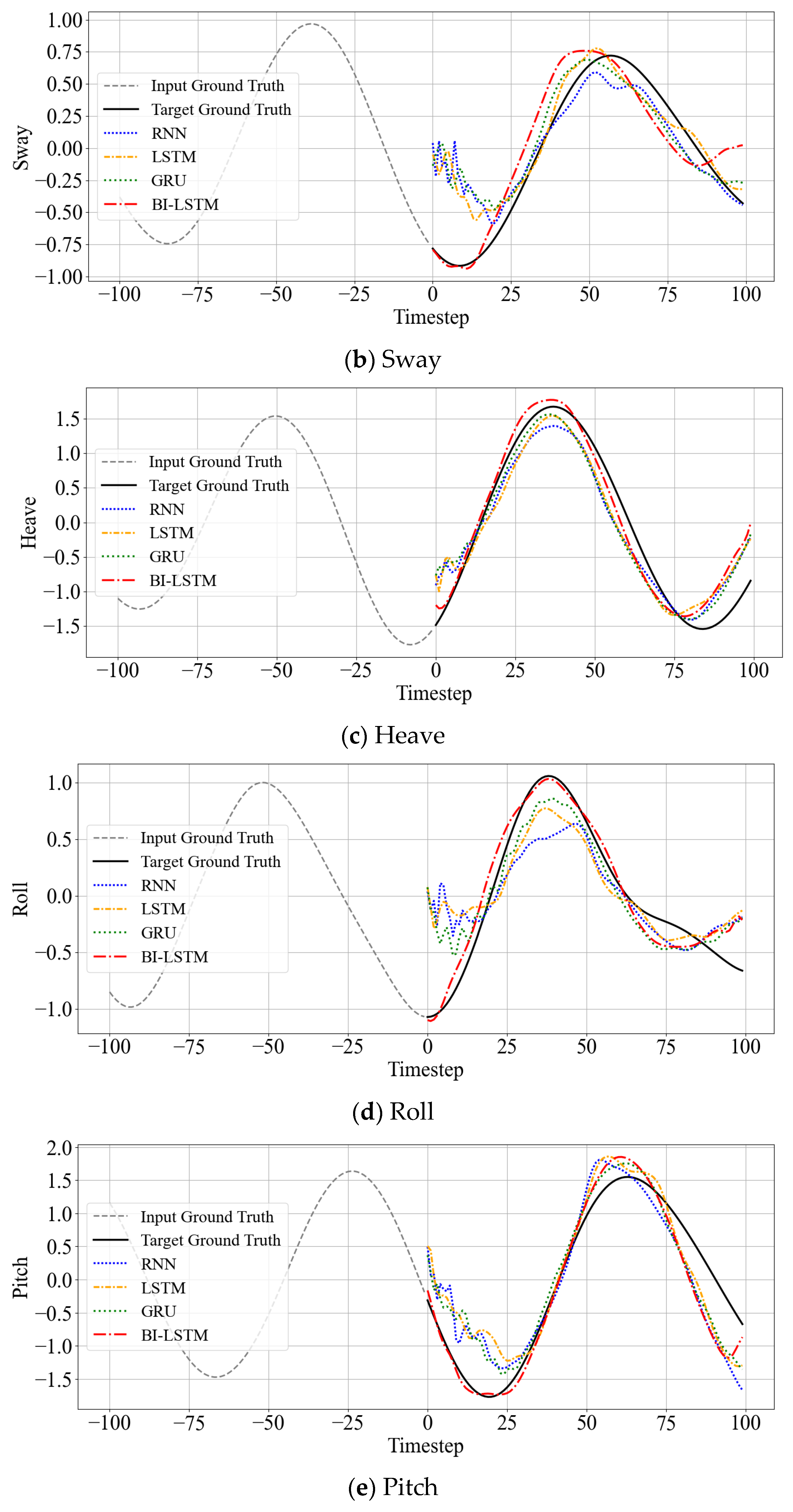
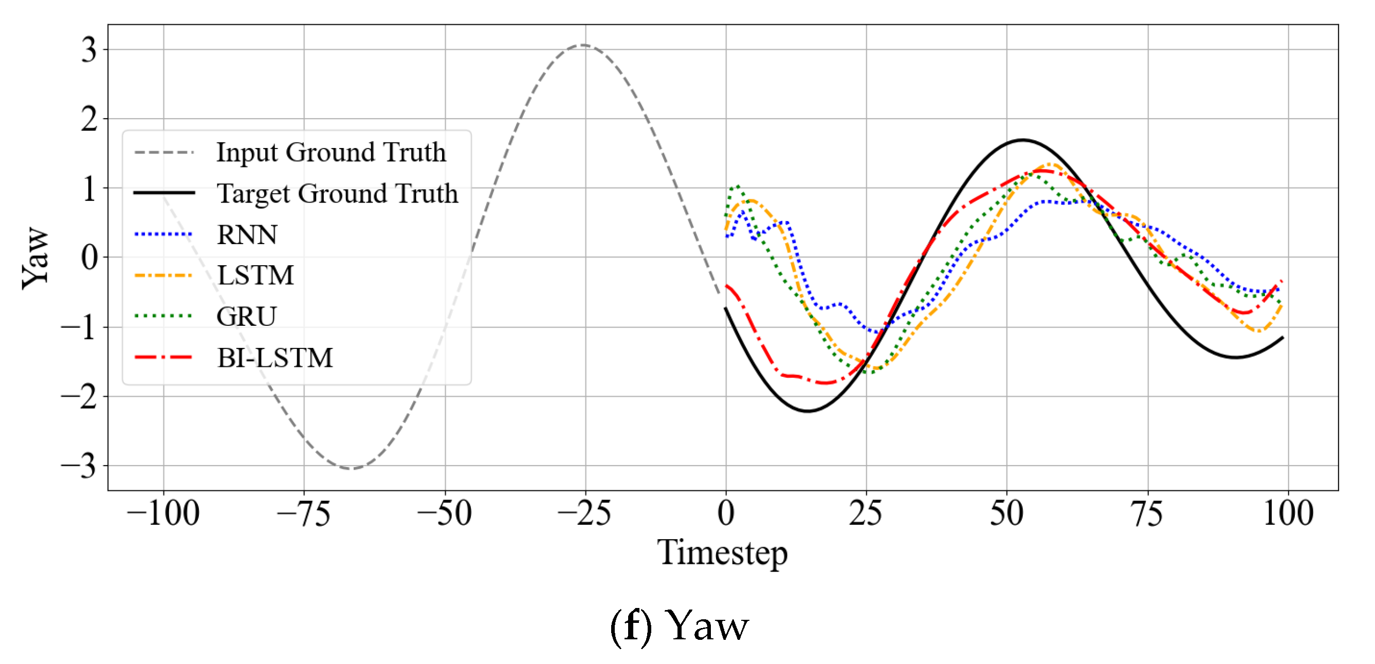
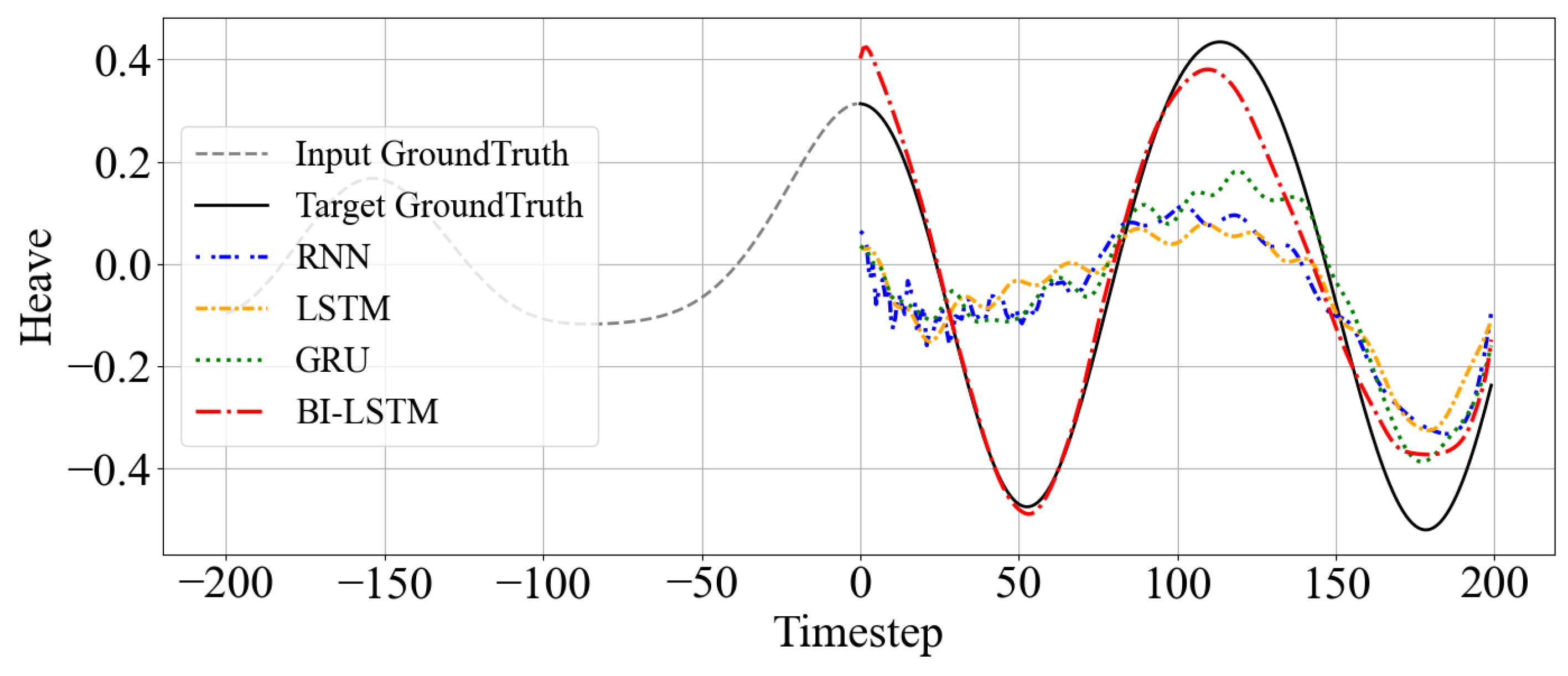
Figure 5 presents a comparative analysis of Mean Squared Error (MSE) across different sequence lengths of 50, 100, 200, 300, and 400. The corresponding actual prediction for each model, arranged from the shortest to the most extended sequence length, are provided in Appendix A (Figure A1a–e) to improve readability while still allowing a comprehensive comparison. The experimental results demonstrate that models achieved remarkably high prediction accuracy up to sequence length 200, confirming the capability of RNN-based models to predict future states up to 20–50 s ahead. However, as sequence length increased beyond this threshold, most models exhibited deteriorating performance, with RNN, LSTM, and GRU models showing particularly pronounced degradation. In contrast, Bi-LSTM maintained relatively stable performance, successfully capturing general time series trends even when sequences extended to 500 timesteps.

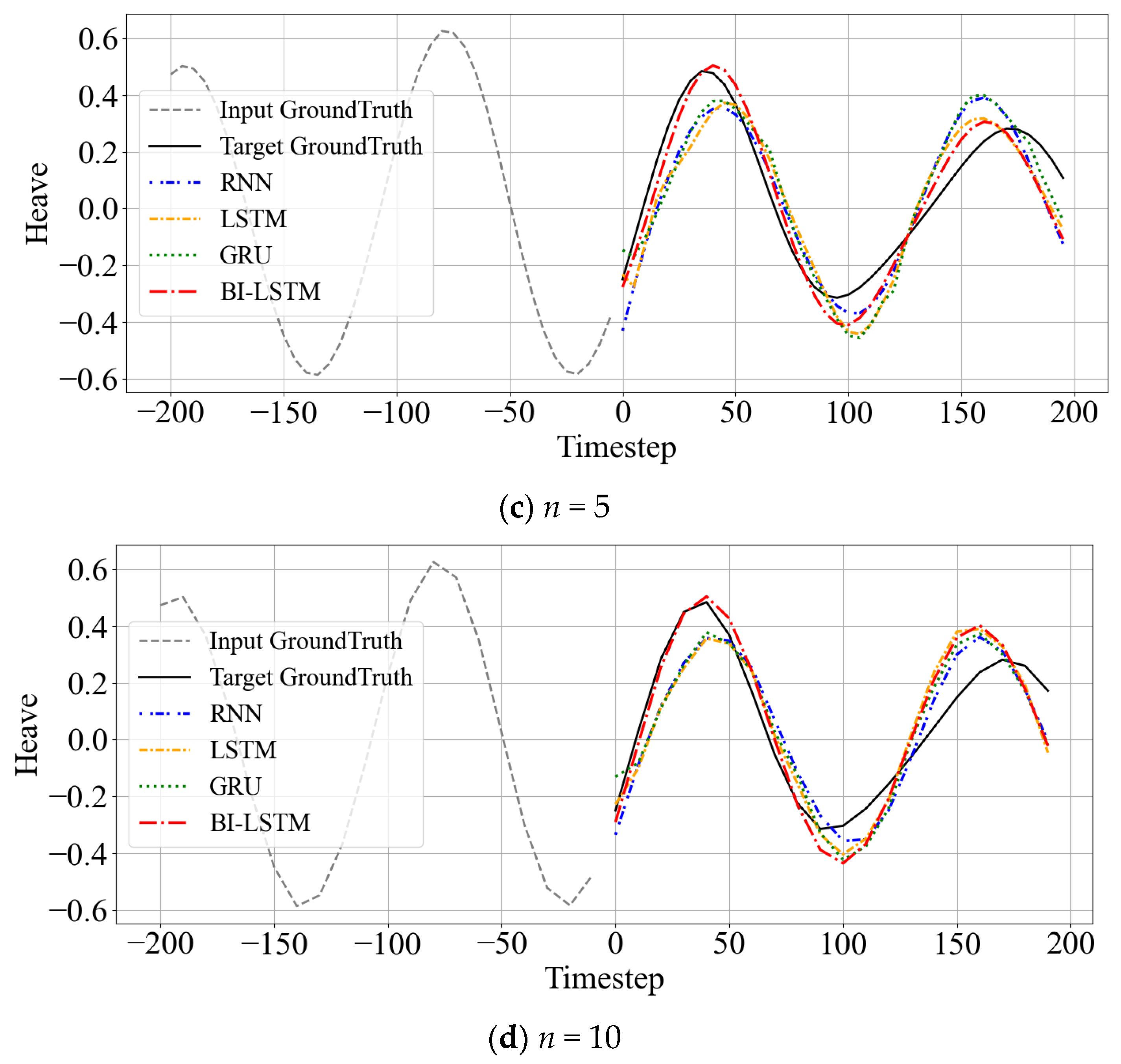
The impact of downsampling on model performance was investigated using intervals n = {1, 2, 5, 10}, with representative results shown in Appendix A (Figure A2a–d) for sequence length 200. The application of downsampling demonstrated a clear trend of enhanced prediction stability through noise reduction. Notably, all models achieved optimal prediction performance under the n = 5 condition, suggesting an ideal balance between information retention and noise suppression.

These findings yield several vital insights for practical applications. First, short-term prediction tasks in single environments can achieve satisfactory performance levels for 20–50 s horizons without requiring complex model architectures. Second, Bi-LSTM demonstrates superior prediction stability and generalization capabilities across sequence lengths and input conditions. Third, appropriate downsampling strategies can significantly enhance prediction performance by filtering high-frequency noise components while preserving essential temporal patterns. These results collectively indicate that even relatively simple model architectures can be effective for single-environment short-term predictions when combined with appropriate preprocessing strategies.

5.1.2. Performance Under Non-Representative Inputs

This section examines how model prediction performance changes when input data inadequately represents the target environment or when dealing with extended time series. Particular emphasis was placed on analyzing predictions from input intervals containing abrupt wave changes or atypical ship motion patterns.

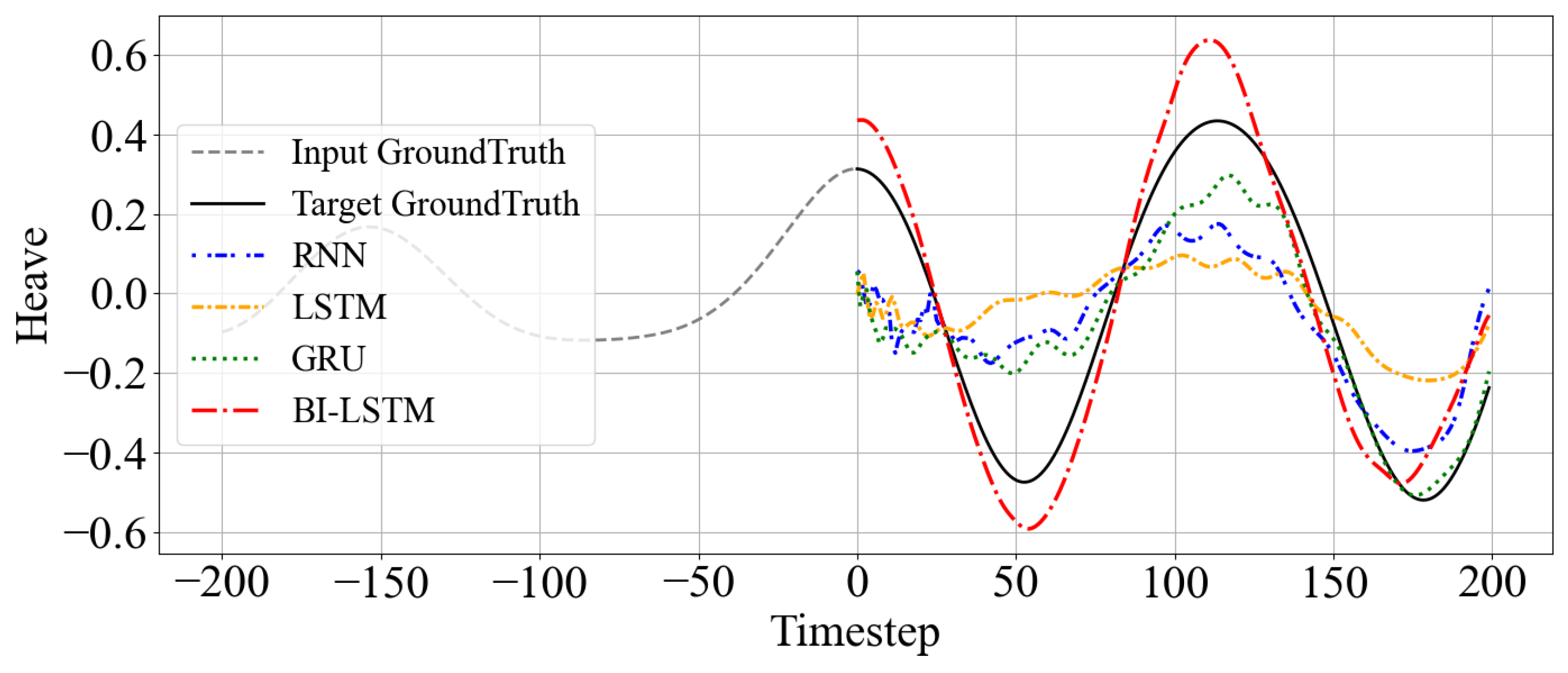
Figure 6 illustrates time series prediction results for atypical input intervals characterized by sudden wave changes. Across this and other non-representative cases, the experimental results consistently reveal significant accuracy degradation across most models. This pattern may suggest that the models did not simply memorize training-specific features, but instead avoided strong overfitting to particular patterns. However, the findings also indicate that uncertainty arising from input variations remains, suggesting the need for training strategies and model interpretations that explicitly account for such uncertainty.

Despite these challenging conditions with insufficient input representativeness, the Bi-LSTM model maintained relatively high prediction accuracy and stable outputs. This superior performance can be attributed to Bi-LSTM’s structural capability to leverage bidirectional temporal information, enabling more accurate predictions simultaneously.

To further investigate prediction performance in non-representative intervals, we conducted additional experiments examining whether model capacity expansion (e.g., hidden nodes: 64 → 128, layers: 2 → 10) could improve performance in these challenging scenarios. Figure 7 visualizes time series prediction results when model sizes were increased for RNN, LSTM, GRU, and Bi-LSTM architectures in environments containing complex waveform variations. Predictions were performed across four different environments, comparing actual values (solid black lines) with each model’s predictions.

RNN, LSTM, and GRU showed partial performance improvements following model expansion. However, these models struggled to capture time series trends during the initial 8 s (80 timesteps) of prediction. Conversely, the expanded Bi-LSTM model demonstrated faster and more accurate predictions, effectively reflecting the amplitude and phase of actual time series from the prediction start point. This indicates that Bi-LSTM can effectively learn meaningful features across sequences and immediately incorporate them into predictions.

5.2. Multi-Environment Generalization Test

The time series prediction models that are generalizable across diverse marine environments have been constructed. To this end, the generalization performance of RNN, LSTM, GRU, and Bi-LSTM-based models was evaluated using data collected from nine marine environmental conditions.

5.2.1. Performance Comparison by Input Features: DOF Combinations and External Variable Effects

The impact of input data configuration on model performance was evaluated when constructing generalizable prediction models across diverse environments. To this end, three different input settings were examined. In the first setting, only a single degree of freedom—heave—was used as input, presented in

Table 5. Experimental setup of input data configurations used to evaluate the impact on prediction model performance across diverse environments.

Input Configuration	Description
Single-DOF	Heave time histories
6-DOF	6-DOF time histories
6-DOF and Wave Elevation	6-DOF time histories and wave elevation at COG

. To capture more comprehensive motion dynamics, the second configuration employed 6-DOF, including roll, pitch, yaw, surge, sway, and heave. In the third configuration, wave elevation data at the center of gravity of the vessel (COG) were incorporated alongside the full 6-DOF input to assess the contribution of external environmental information to the overall prediction accuracy.

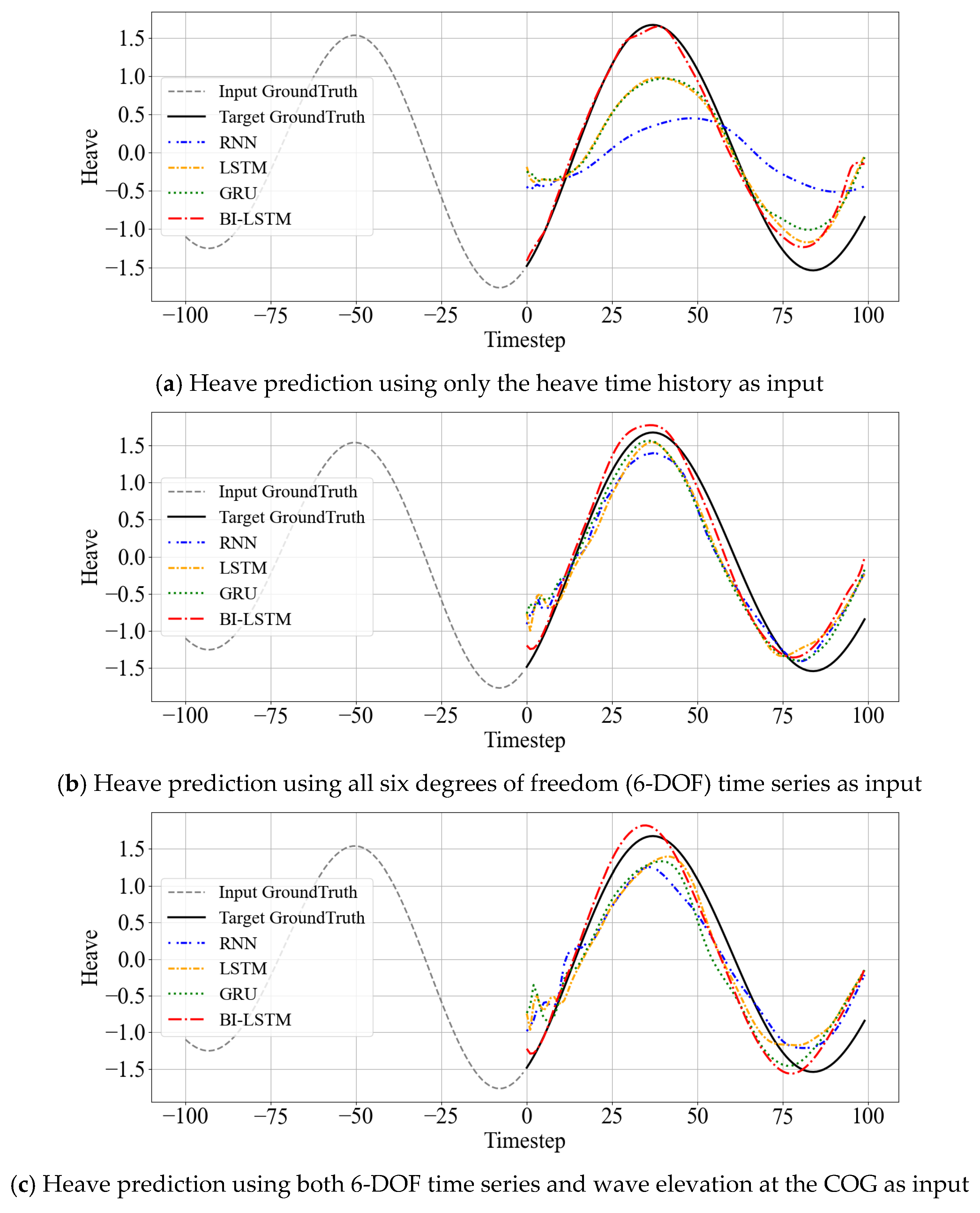
Figure 8 illustrates the variation in heave prediction results depending on the input configuration. Panel (a) presents the prediction based on the heave time history as the sole input. Panel (b) shows the results when all 6-DOF time series are used as input, while panel (c) depicts the prediction obtained when both the six-DOF time series and wave elevation at the COG are provided as inputs. All predictions were evaluated over the same test time intervals, using models with an identical architecture consisting of a hidden size of 64 and two layers. 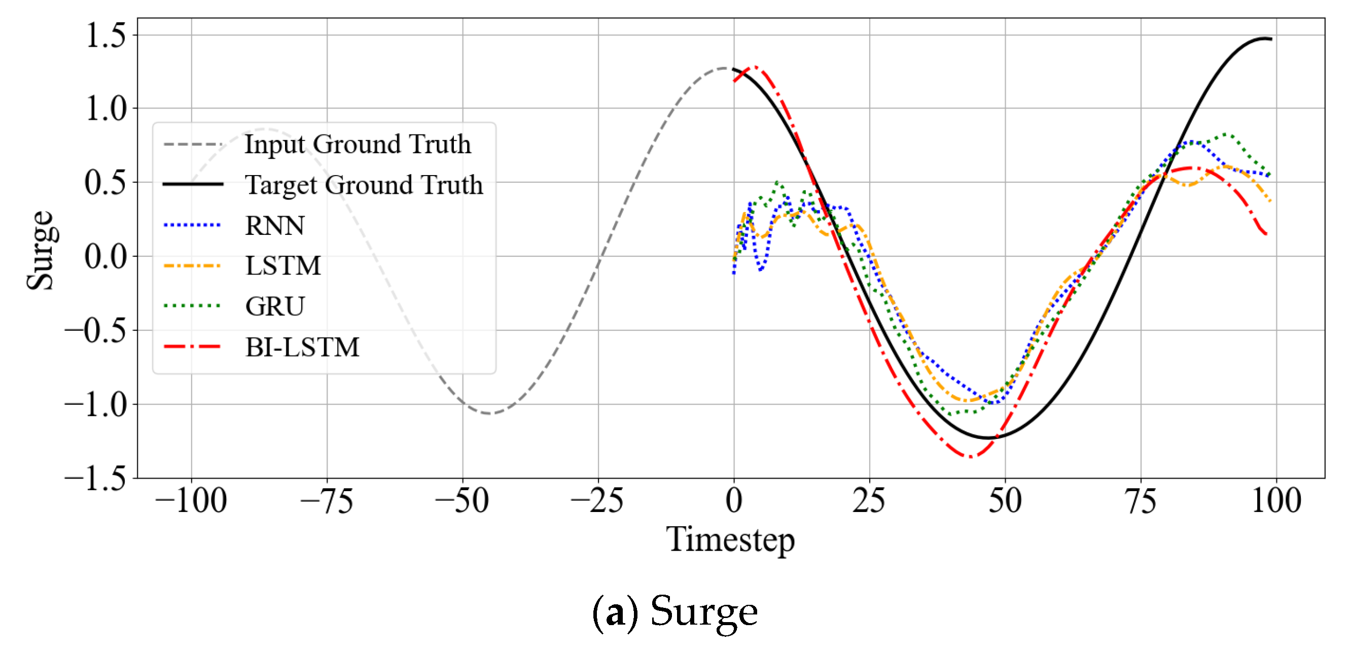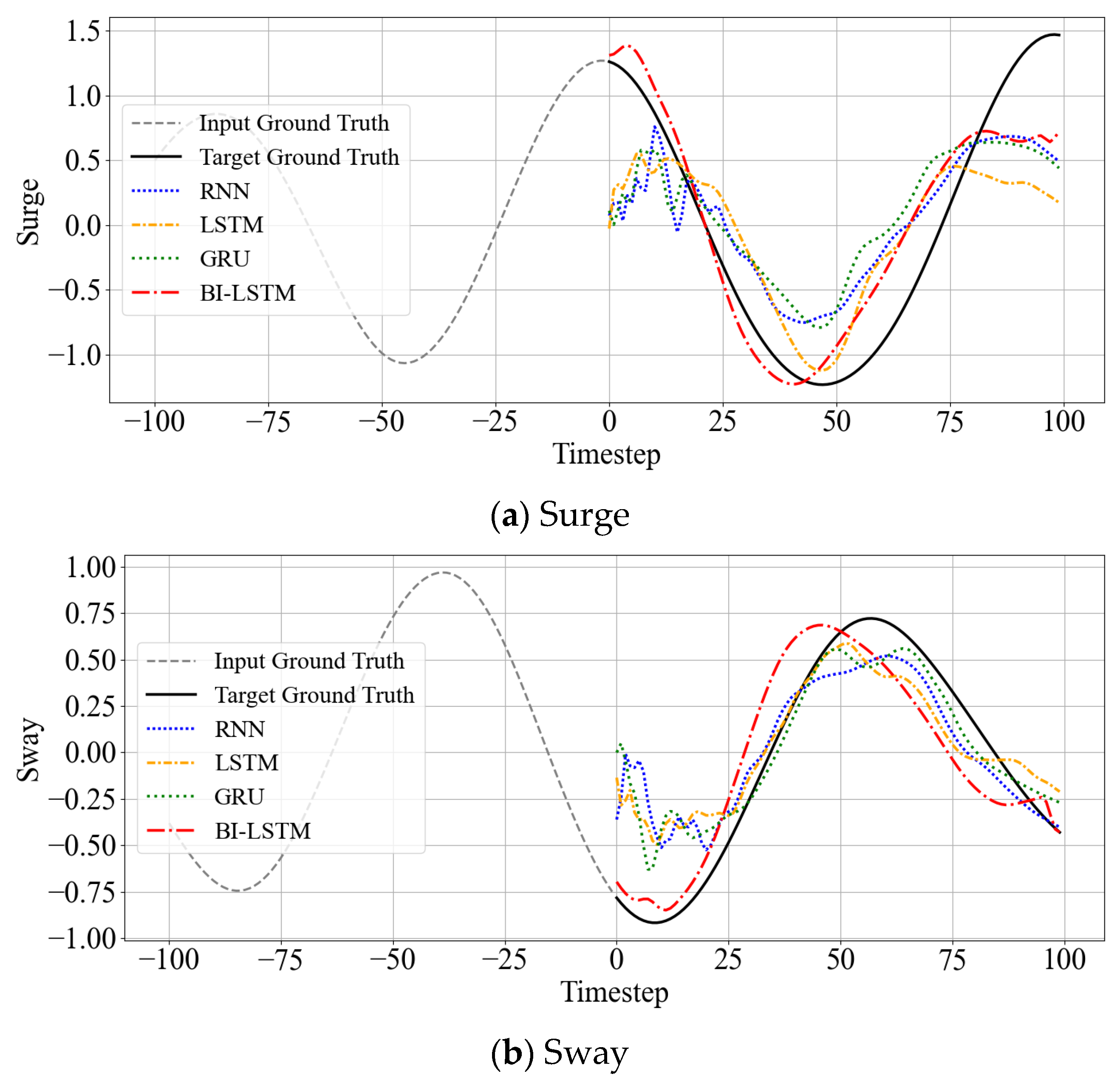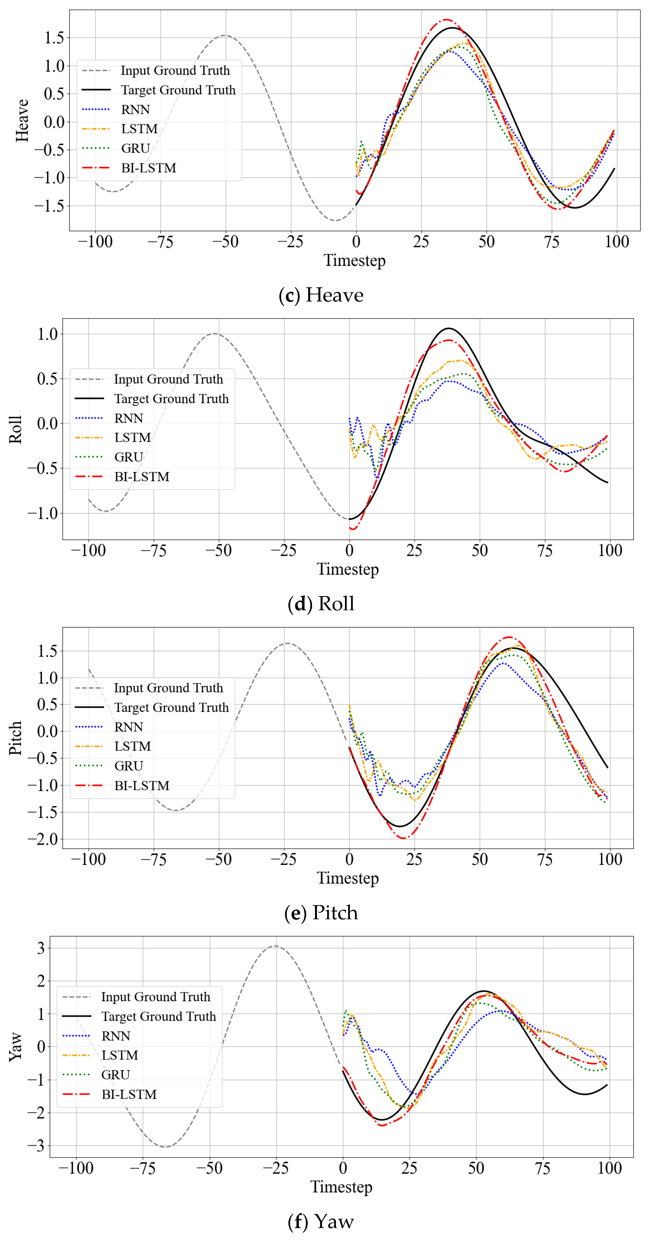For clarity, Figure 8 presents only the heave prediction results as a representative case for comparison. The complete prediction results for all six DOFs (surge, sway, heave, roll, pitch, and yaw) under the different input configurations are provided in Appendices B.1 (Figure A3a–f) and B.2 (Figure A4a–f). These supplementary results confirm that the performance patterns observed in heave prediction are consistently reflected across the other DOFs.

Experimental results showed that using all 6-DOF as input consistently demonstrated superior prediction performance compared to single DOF input. This is interpreted as the physical associations and correlations between DOFs being effectively learned in RNN-based models. For example, Roll or Pitch movements have close correlations with Heave changes, and such linked information contributes to improved prediction accuracy.

Conversely, prediction performance deteriorated in some environments when wave data was added. While wave data is an exogenous variable affecting DOF, it may lack explicit predictable patterns or include time-lagged and nonlinear relationships. Particularly, waves often affect DOF with time delays, potentially leading to confusion rather than sufficient reflection in simple sequential models.

These results suggest that input configurations with direct and explicit correlations are advantageous for prediction performance improvement in simple time series models. By contrast, incorporating exogenous variables such as wave elevation introduced mixed effects in our tested cases, possibly due to time-lagged or nonlinear relationships. This observation indicates that effectively leveraging such variables may require more advanced model structures or additional mechanisms, and further investigation is needed to confirm this across diverse settings.

5.2.2. Sensitivity to Sequence Length

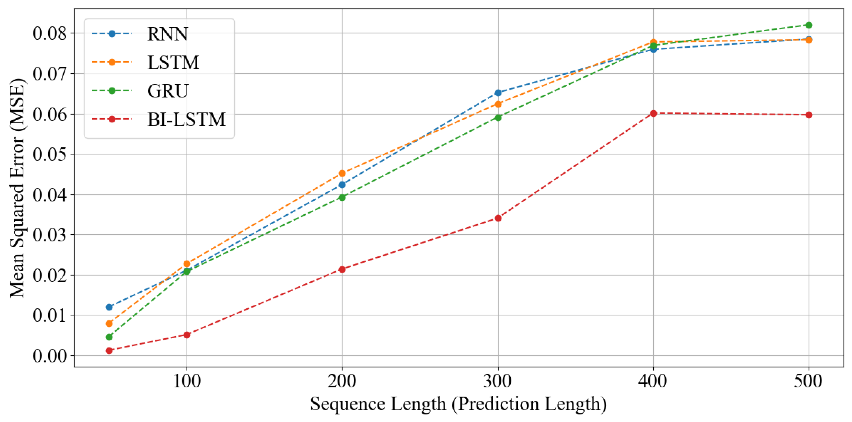
Time series prediction performance sensitivity to input sequence length variations was analyzed. The experiments used four models (RNN, LSTM, GRU, Bi-LSTM), with input data and prediction targets set to 6-DOF. Sequence lengths were set as 50, 100, 200, and 300 timesteps, with analysis focused on average prediction error (MSE) and actual prediction curves.

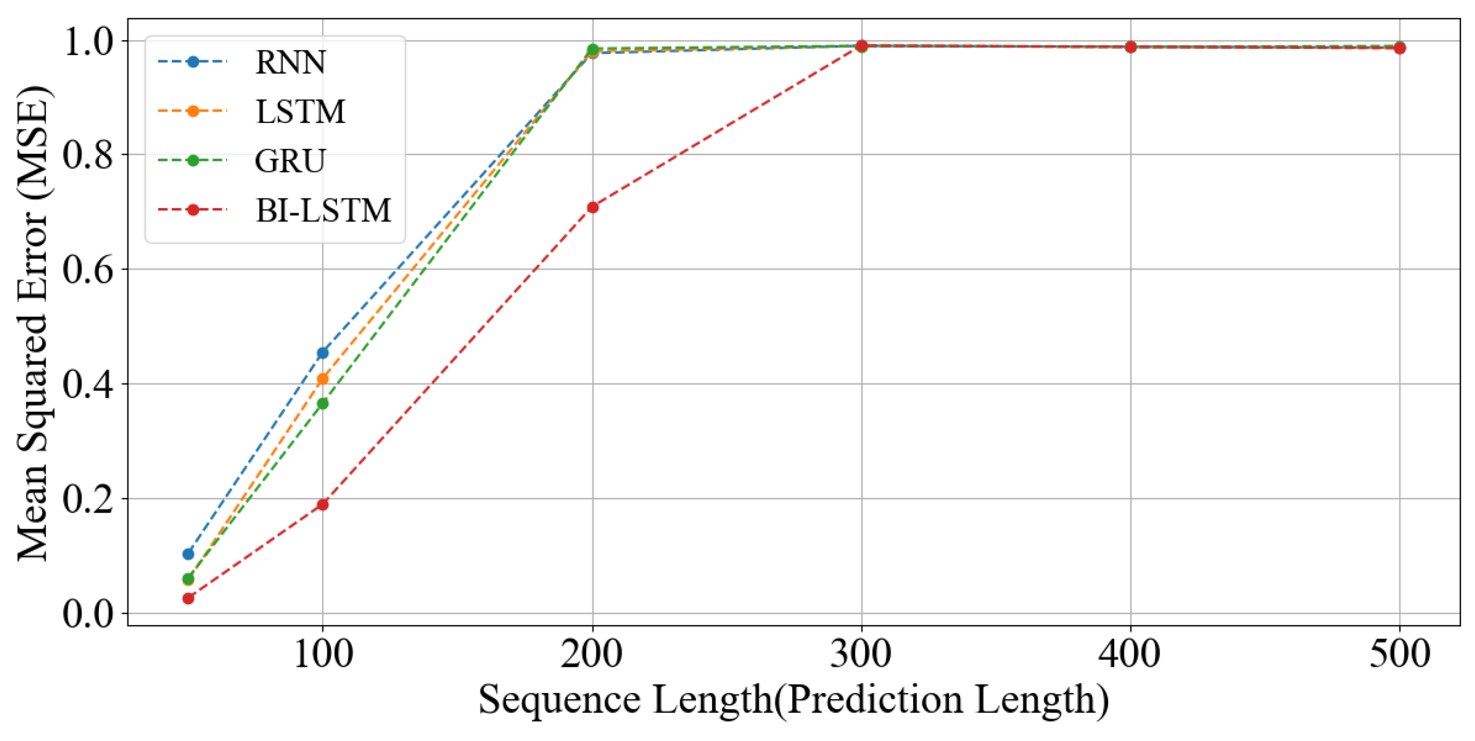
Figure 9 compares average MSE values for each sequence length. When sequence length increased beyond 200 timesteps, prediction performance deteriorated sharply in most models. This suggests structural limitations in RNN-based models for effectively learning long-term time series dependencies and potential information loss accumulation or gradient vanishing problems as sequences lengthen. RNN, LSTM, and GRU models showed significantly decreased MSE values beyond sequence 200 timesteps, while Bi-LSTM maintained relatively stable performance, demonstrating structural superiority.

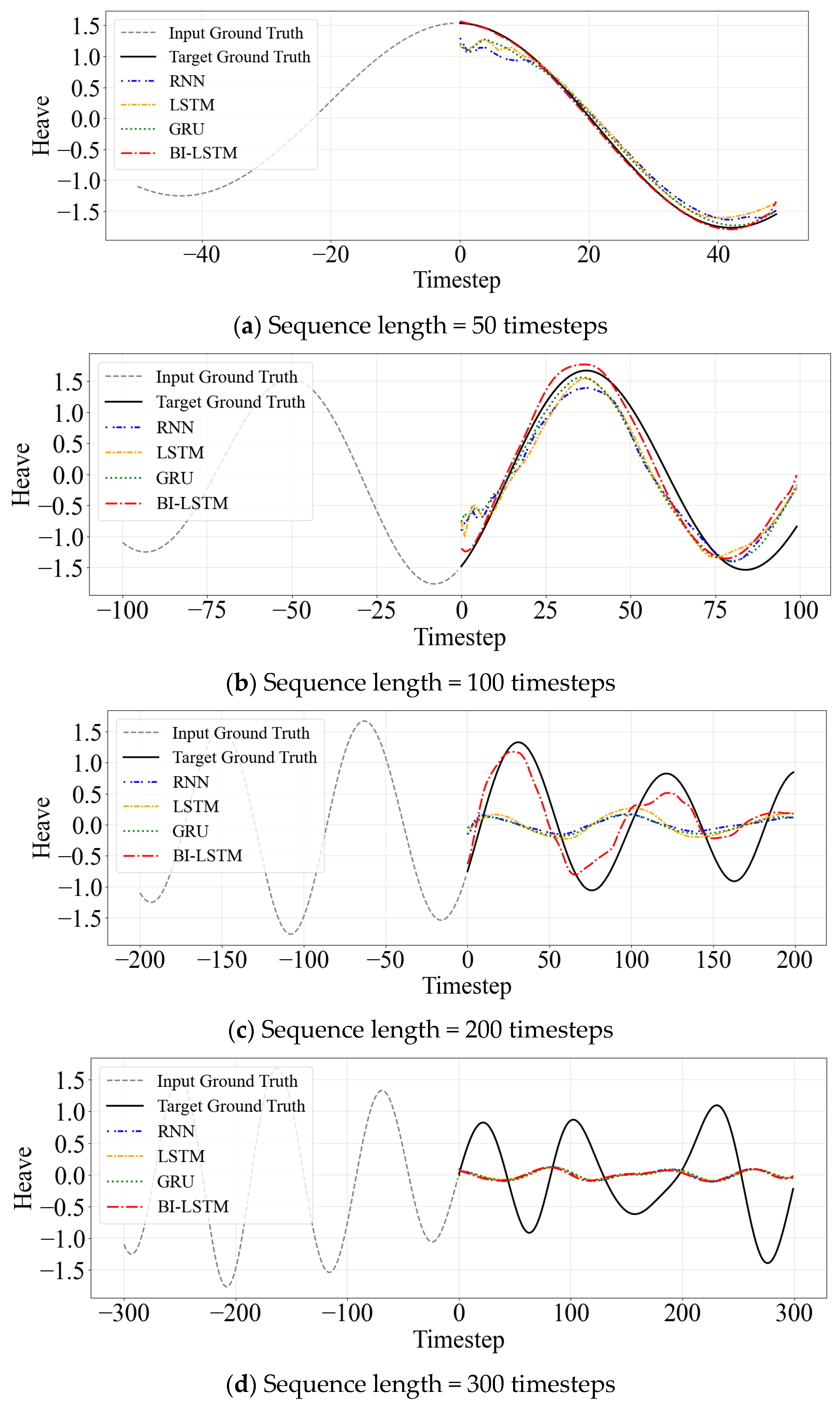
Figure A5a–d in Appendix B visualizes actual prediction curves under identical conditions. While most models followed overall time series flow in short sequences of 50 and 100, RNN, LSTM, and GRU models showed near-prediction failure results in long sequences of 200 and 300. Only Bi-LSTM reproduced relatively accurate predictions even in long sequences, though overall accuracy decreased somewhat compared to shorter sequences. This suggests that while Bi-LSTM enables more effective long-term dependency processing than other RNN models, excessively long input sequences may negatively impact prediction accuracy through unnecessary information.

Consequently, increasing sequence length does not directly lead to improved prediction performance, demonstrating the importance of balanced adjustment between input sequence length and model structure. Particularly in time series prediction problems where long-term dependencies are essential, such as complex marine environments, bidirectional structures like Bi-LSTM can provide more robust performance.

5.2.3. Sensitivity to Down-Sampling

High-resolution time series data inherently contains high-frequency noise components that can impair model generalization and induce overfitting. Downsampling represents a fundamental preprocessing technique to mitigate these challenges by strategically reducing temporal resolution while preserving essential dynamic patterns. This section investigates the effects of varying downsampling intervals on Bi-LSTM prediction performance using a fixed sequence length of 200 timesteps and downsampling intervals n = {1, 2, 5, 10}.

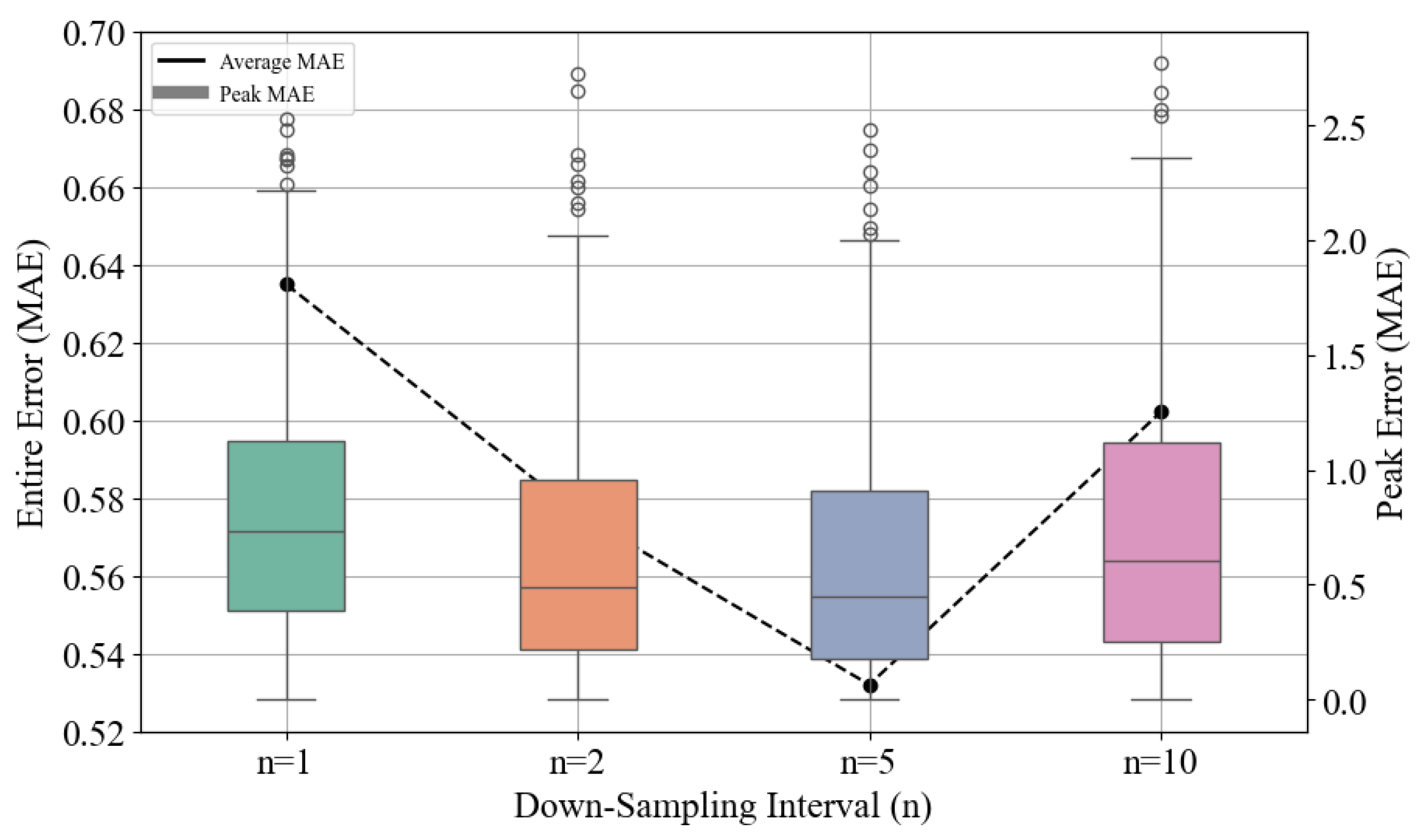
Figure 10 presents the Mean Absolute Error (MAE) analysis across different downsampling intervals, comparing both overall time series errors and errors specifically at peak points, which hold critical physical significance in ship motion dynamics. The peak point errors are presented as box plots using the right y-axis, while the overall time series errors are shown as a black dashed line using the left y-axis. The results demonstrate that appropriate downsampling effectively filters high-frequency noise, enabling models to focus on fundamental time series structures and thereby enhancing prediction accuracy. The optimal performance was achieved at n = 5, recording the lowest errors for overall and peak point predictions. However, excessive downsampling at n = 10 led to performance degradation due to the loss of essential waveform information. This finding suggests that sampling intervals exceeding 1 s may prevent models from adequately capturing crucial temporal patterns.

As shown in

Table 6. t-test results comparing ground truth and predicted peak values (BI-LSTM, n = 5).

	Values
Mean (Ground Truth)	0.0057
Mean (Prediction)	−0.0106
T-Statistic	0.3629
p-value	0.7169

, a paired t-test between ground truth and predicted peak values under the optimal downsampling condition (n = 5) yielded a non-significant result (t = 0.363, p = 0.717 > 0.05). This indicates that predicted peaks are statistically indistinguishable from actual values, validating the model’s ability to reproduce peak dynamics without systematic bias.

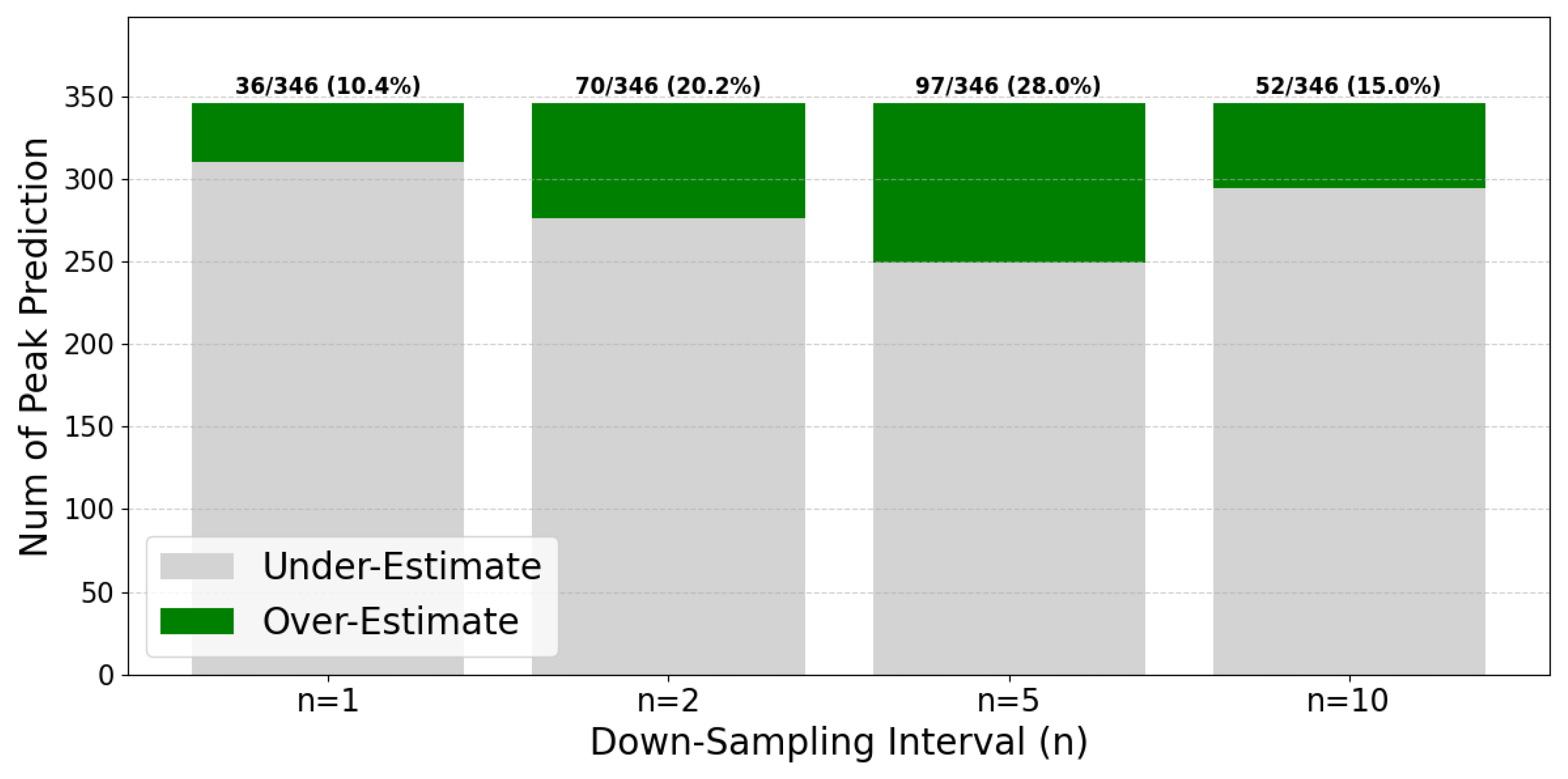
The analysis of prediction directionality provides additional insights into model behavior. Figure 11 compares the Overestimated Peak Ratio across downsampling intervals, quantifying the proportion of predicted peaks exceeding actual values. In marine applications, overestimation is generally preferable to underestimation from a vessel control perspective, as it enables more conservative operational decisions. The n = 5 condition exhibited the most stable overestimation ratio, indicating that the model maintains appropriately conservative predictions while achieving optimal accuracy.

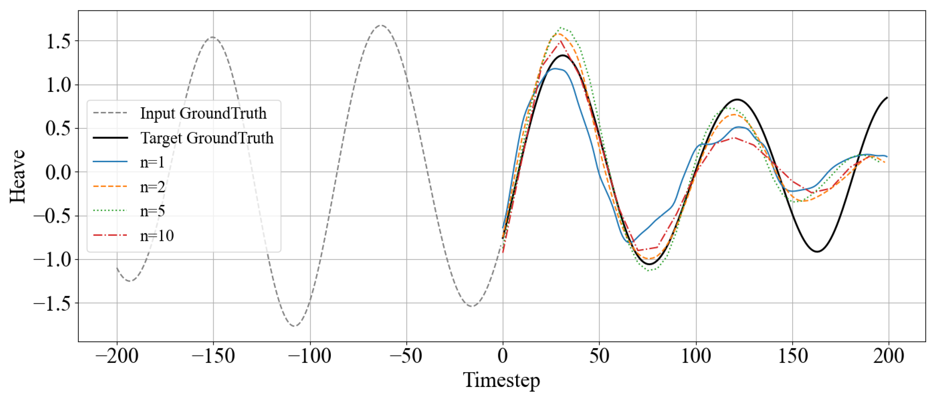
Figure 12 provides a visual comparison of prediction curves under different downsampling conditions. Consistent with the quantitative analysis, the n = 1 condition exhibited rapidly fluctuating prediction curves due to unfiltered high-frequency noise. Conversely, the n = 10 condition showed degraded performance compared to n = 2 and n = 5. The n = 5 condition achieved an optimal balance, maintaining waveform similarity to actual data while minimizing noise and securing prediction stability and accuracy.

These findings collectively demonstrate that strategic downsampling, rather than direct utilization of high-resolution data, significantly contributes to prediction performance enhancement. The results emphasize that appropriate data preprocessing is crucial in addressing complex, high-dimensional time series prediction challenges of marine environments.

5.2.4. Effect of Model Upsizing on Multi-Environment Generalization

To improve generalization performance across diverse marine environments, this section examines the impact of systematic model architecture expansion on prediction capabilities. All experiments utilized 6-DOF (Surge, Sway, Heave, Roll, Pitch, Yaw) time series data for both input and output, with a fixed 20 s prediction horizon and the optimal downsampling interval of n = 5 established in previous experiments. Model scaling was implemented through progressive expansion of hidden nodes (64, 128, 256, 512) and layer depth (2, 3, 5, 10, 15, 20).

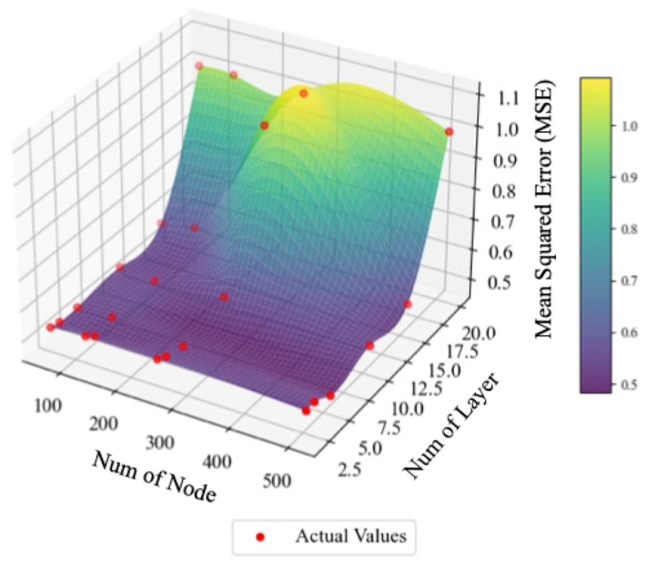
Figure 13 visualizes the three-dimensional relationship between model architecture parameters and prediction performance for the Bi-LSTM model. The surface plot illustrates average RMSE variations as functions of hidden node count and layer depth, with each data point representing averaged results from repeated experiments under identical conditions. The analysis reveals that prediction performance generally improved with increasing layer depth up to 15 layers, beyond which performance deteriorated significantly at 20 layers. This pattern suggests that excessive network depth introduces optimization challenges that compromise generalization capabilities. Similarly, increasing hidden nodes contributed to performance improvements up to 256 nodes, with diminishing returns beyond this threshold. These observations underscore that simple parameter multiplication does not guarantee performance enhancement and highlight the critical importance of balanced architectural design.

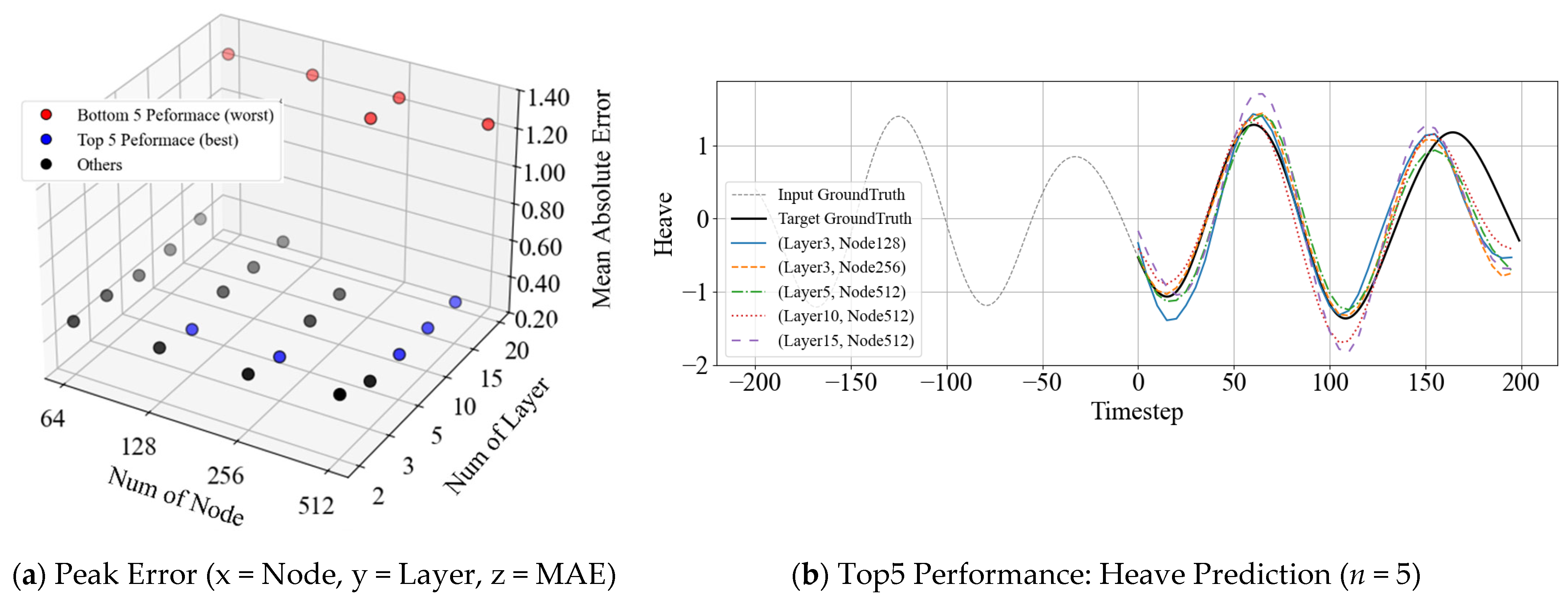
Figure 14 evaluates model configurations based on physical peak errors (MAE at local maxima) for more nuanced analysis, identifying top-performing architectures. Figure 14a maps peak error measurements across different layer and node configurations, with the five worst-performing models highlighted in blue and the five best-performing models in red. Figure 14b presents prediction curves from the top five models, demonstrating their ability to accurately reproduce the ground truth data’s amplitude and phase characteristics. The curves are shown in different colors, with the number of layers and nodes for each model indicated.

As shown in

Table 7. t-test results comparing ground truth and predicted peak values (BI-LSTM, n = 5, Layer= 15, Node = 512).

	Values
Mean (Ground Truth)	0.0078
Mean (Prediction)	−0.0002
T-Statistic	0.2156
p-value	0.8294

, the enlarged Bi-LSTM architecture (15 layers, 512 nodes) yielded a paired t-test result that was statistically non-significant (t = 0.216, p = 0.829 > 0.05), consistent with the smaller model in Table 6. This finding indicates that increasing model capacity does not introduce systematic bias, and peak predictions remain statistically aligned with the ground truth.

6. Discussion

The experimental results provide insights into the capabilities and limitations of RNN-based models for ship motion prediction across varying marine environments. The observed differences in prediction performance between single and multi-environment scenarios warrant further examination of the underlying factors affecting model generalization.

In addition to the heave motion, the other five motion components (surge, sway, roll, pitch, and yaw) were analyzed. The results demonstrated that the trends observed for heave, such as the relative stability of Bi-LSTM and the effects of sequence length and downsampling, were consistently reproduced across all 6DOF motions. Therefore, only heave is shown in the main text for clarity, while the findings represent all motion components.

The reduction in prediction horizon from over 40 s in single-environment conditions to approximately 20 s in multi-environment scenarios suggests that model complexity increases substantially when attempting to capture diverse maritime dynamics. This performance gap may be attributed to the increased variability in wave patterns, vessel responses, and environmental conditions across different scenarios. The sharp degradation observed when input data poorly represent the training distribution indicates that these models rely heavily on learned ecological patterns, which may limit their applicability in highly variable operational conditions.

The superior performance of multi-DOF inputs compared to single DOF inputs aligns with the physical understanding of ship dynamics, where motions in different degrees of freedom are inherently coupled. The correlations between roll, pitch, and heave, for instance, reflect the integrated response of the vessel to wave excitation. However, the unexpected performance degradation with wave height inclusion requires careful interpretation. While D’Agostino et al. (2022) [44] attributed similar observations to measurement location issues, our results suggest that the relationship between wave measurements and vessel response may be more complex than what simple sequential models can capture. This could involve nonlinear wave-structure interactions, frequency-dependent transfer functions, or spatial variations in wave fields not adequately represented in point measurements.

The performance characteristics across sequence lengths and downsampling intervals reveal fundamental trade-offs in time series modeling. The degradation beyond 200 timesteps may reflect the well-documented vanishing gradient problem in RNNs, though the relatively better performance of Bi-LSTM suggests that bidirectional processing partially mitigates this issue. The optimal downsampling interval of n = 5 likely represents a balance between preserving motion dynamics (at relatively low frequencies for ship motions) and filtering high-frequency measurement noise. The performance variations across different downsampling intervals are evident in the MAE results (Figure 12) and the corresponding prediction curves’ comparisons (Figure 8 and Figure 14). These findings suggest that moderate downsampling may not significantly degrade model performance, providing a rationale for balancing sampling frequency and data storage requirements in system design.

It is observed that increasing the number of layers and units in Bi-LSTM tends to improve prediction performance (Figure 13), which aligns with previous findings that highlight the contribution of LSTM/Bi-LSTM model capacity to generalization in time series forecasting tasks [61]. The optimal configuration of 256 hidden nodes and 15 layers for Bi-LSTM may represent a sweet spot where the model has sufficient capacity to capture complex patterns without overfitting to training data specifics. The performance degradation beyond these thresholds could indicate optimization difficulties associated with intense networks or memorizing training data patterns that do not generalize well.

The introduction of Peak Matching as an evaluation metric addresses a specific limitation of MSE-based assessments in the context of ship motion prediction. While MSE provides an average measure of error, it does not capture the accuracy of extrema prediction. It is often more critical for safety-critical operational decisions such as cargo handling, collision avoidance, helicopter operations, or structural load assessments. The strength of the Peak Matching metric lies in its intuitive interpretability and ability to highlight dynamics directly relevant to maritime safety. Nevertheless, its effectiveness may depend on the specific application context, and future validation with real-world operational data will be necessary to establish its full utility. In particular, future work may include rigorously validating this metric using operational datasets to ensure its practical relevance.

Several limitations of this study should be acknowledged. First, the experiments were conducted on a simulated dataset of a specific vessel (KCS model) under nine sea states. Although this setting considers a range of wave environments, it inherently limits the generalizability of the findings to different vessel types and real-world maritime conditions. Therefore, future validation with measurement data from sea trials or operational environments will be essential to confirm the robustness of the models. Second, the scope of model architectures was deliberately limited to RNN-based variants to establish a clear and consistent comparative baseline. This choice reflects the recent surge of research activity in artificial intelligence-driven approaches, and the study focused exclusively on fundamental RNN-based architectures. Traditional methods such as ARIMA, Kalman filtering, and physics-based models were not considered within the present scope. Nonetheless, emerging techniques—such as attention mechanisms, Transformer-based networks, and physics-informed neural architectures—may provide enhanced capabilities for capturing complex nonlinear vessel–wave interactions. Third, the analysis was restricted to deterministic predictions without explicit quantification of predictive uncertainty, which represents a valuable direction for future work in support of risk-informed decision-making.

These findings suggest several directions for improving ship motion prediction systems. The challenges with exogenous variables indicate a need for more sophisticated approaches to handle asynchronous or spatially distributed measurements. The performance patterns across different architectures suggest hybrid approaches combining physics-based models with data-driven components might better capture the underlying dynamics. Additionally, developing uncertainty quantification methods would enhance the practical utility of these predictions in operational contexts where risk assessment is crucial.

7. Concluding Remarks

This study investigated neural network–based time series prediction models for ship motion forecasting under varying environmental and input configurations. Several academic contributions and engineering implications can be articulated based on a comprehensive set of experiments.

First, the study established the first unified baseline for full 6-DOF ship motion prediction by systematically comparing four representative RNN-based architectures (RNN, LSTM, GRU, Bi-LSTM) under both single- and multi-environmental conditions. In addition, two complementary evaluation metrics, Peak Matching and the Overestimation Ratio, were proposed to extend conventional error measures such as MSE and MAE by explicitly capturing the accuracy and tendencies of extrema prediction, which are critical in safety-sensitive maritime contexts. Furthermore, practical design guidelines were derived regarding sequence length, downsampling strategies, model capacity, and input dimensionality, providing actionable insights for selecting and configuring models in different operational scenarios.

From an engineering perspective, accurately predicting peak motions directly affects navigation safety, including cargo handling, collision avoidance, helicopter operations, and structural load management. The proposed evaluation framework underscores the importance of conservative forecasting, where overestimation may be preferable to underestimation for risk mitigation. Moreover, the trade-offs identified in sequence length, downsampling, and model scaling offer practical references for implementing ship motion forecasting systems that balance accuracy, computational efficiency, and robustness.

The experimental results further highlight several key findings. Prediction horizons varied between approximately 40 s in single-environment settings and about 20 s in multi-environment settings, illustrating the increased complexity of generalized forecasting. Multi-DOF inputs generally enhanced prediction performance relative to single-DOF inputs, while including wave data yielded mixed results. The Bi-LSTM architecture demonstrated relatively stable performance across diverse conditions, and moderate downsampling (n = 5) improved predictive accuracy. At the same time, model scaling exhibited diminishing returns beyond specific architecture sizes, with optimal configurations appearing to be task dependent.

Looking ahead, validation with full-scale measurement data will be essential to confirm model robustness in real-world applications. Hybrid modeling frameworks that combine physical models with data-driven learning offer a promising direction for better capturing nonlinear vessel–wave interactions. Furthermore, incorporating uncertainty quantification into predictive outputs could strengthen risk-informed decision-making in safety-critical maritime operations.

This study advances methodological and practical insights into ship motion forecasting. Emphasizing peak-based evaluation and systematically comparing RNN-based models under diverse conditions provides a rigorous foundation for future developments in hybrid, data-driven, and risk-aware prediction frameworks that enhance maritime safety and operational reliability.