Abstract
The assessment of ship dynamic stability in waves is crucial for navigation safety. To mitigate accidents, the International Maritime Organization (IMO) has formulated corresponding technical standards. However, evaluating the dynamic stability performance of ships involves complex numerical simulation or model experiments based on hydrodynamic methods, which demands professionalism, substantial time, and significant financial cost. This paper analyzes the feasibility of using the Generalized Regression Neural Network (GRNN) method to build a surrogate model for ship dynamic stability performance calculation. Comparisons with hydrodynamics-based simulations reveal that the surrogate model matches the trends well, yet the root-mean-square error (RMSE) remains non-negligible. Therefore, an improved GRNN surrogate model is proposed to solve this problem. By incorporating enhanced feature preprocessing and clustering techniques, the improved model not only increases predictive accuracy but also achieves significant efficiency gains, reducing the computational time from days or weeks for numerical simulations to seconds or minutes. Experimental results show that the improved surrogate model outperforms the baseline GRNN model, and this framework can serve as a practical surrogate for hydrodynamics-based numerical models to rapidly assess pre-voyage dynamic stability.
1. Introduction
Container ships sailing at sea are exposed to irregular motions characterized by nonlinearity and non-stationarity, induced by extreme weather, wind, waves, and currents, which significantly increase navigational risks [1]. For example, in late October 1998, a fully loaded post-Panamax C11 container ship “APL CHINA” sailed eastward from Kaohsiung to Seattle, encountered a severe storm in the North Pacific and experienced pronounced parametric roll, which caused extensive cargo collapse and severe economic losses. To mitigate such risks, The International Maritime Organization (IMO) promulgated the second-generation intact stability (SGIS) standards [2] in 2020, which encompass the primary stability failure modes in waves: parametric roll (PR), pure loss of stability (PL), excessive acceleration (EA), dead ship condition and surf-riding. These standards introduced safety requirements and numerical approaches for the evaluation of dynamic stability in waves: once the loading condition is determined, stability may be assessed either by hydrodynamics-based simplified vulnerability criteria [3,4], or by higher-fidelity time-domain numerical simulations [5,6,7,8].
Viscous-flow computational fluid dynamics (CFD), founded on the continuity equation and the Navier–Stokes equations, is capable of resolving viscous effects on flow structures and velocity distributions with high accuracy, thereby demonstrating significant advantages in simulating complex ship-flow fields. For instance, Liu et al. employed the URANS method to realize, for the first time, full-scale high-accuracy CFD simulations of parametric roll, effectively avoiding model-scale effects [9]; Huang et al. used CFD to evaluate seakeeping performance in bi-directional beam seas and regular waves [10]; and Kim et al. conducted CFD-based investigations into ship maneuverability under different current conditions [11]. These studies collectively confirm the validity and methodological rigor of CFD.
Nevertheless, in engineering applications, relying solely on CFD or other high-fidelity numerical/experimental methods for large-scale condition assessment still presents three major bottlenecks.
- (1)
- High computational cost: mesh resolution and free-surface capturing sharply increase computational demand; even under O(102)-core parallel conditions, a single case often requires days to weeks, making rapid iteration and batch evaluations impractical.
- (2)
- Modeling and solution complexity: six-degree-of-freedom coupling and turbulence–free-surface interactions substantially increase algorithmic complexity, imposing stringent requirements on hardware and operator expertise.
- (3)
- Coverage limitations: phenomena such as parametric roll are highly sensitive to loading parameters such as draft, trim, and vertical center of gravity (KG), while operational loading patterns exhibit high-dimensional, discrete distributions; thus, existing frameworks cannot exhaustively cover all cases, constraining comprehensive design-stage verification and timely operational-stage risk assessment.
Even with potential flow theory, although computational speed improves, the approach remains inadequate for large-scale coverage and near-real-time decision-making, and is still highly labor-intensive.
As the maritime industry progresses toward intelligent and unmanned shipping, safety assessment and route planning require automated, rapid, and robust capabilities. In particular, the strong nonlinearity and high sensitivity of ship dynamic stability to loading, operational, and environmental conditions lead to high-dimensional, large-scale, and complex data structures, where simplified methods such as tabulated interpolation cannot capture the essential dynamics [7]. This motivates the exploration of data-driven surrogate models that can provide rapid approximations to high-fidelity solutions while maintaining physical consistency.
To meet this demand, existing studies can broadly be categorized into two directions. The first line of research is short-term time-series-oriented, focusing on motion extrapolation from continuous observations and capturing long-range dependencies. For example, Zhang et al. developed a hybrid model that integrated a CNN, an MRNN and IADPSO to predict the ship pitch, roll, and heave motions. The CNN is used to extract the spatial features from the ship data of the time series, and then the MRNN is used to extract the temporal features of the new time series, and finally, the IADPSO algorithm is used to optimize the hyper-parameters of the CNN-MRNN model for accurate prediction [12]. Li et al. uses a sequence-to-sequence approach for short-term prediction of ship roll motion using a Bidirectional Long Short-Term Memory Network (Bi-LSTM) with teacher forcing [13]. Li et al. proposed a method combining phase space reconstruction theory with an improved Elman neural network to predict ship roll motion, demonstrating higher accuracy compared to using the Elman network alone [14]. Li et al. proposed a ship roll motion prediction model based on an NARX neural network with wind speed and direction as external inputs, which demonstrated higher accuracy compared to a BP neural network in experimental validations [15]. Peña et al. uses two and three hidden layer structure ANN models to realize the time series prediction of the ship’s transverse rocking motion, and through experiments, it is concluded that the accurate prediction can be realized 40 s ahead of time in simple cases and 10 s ahead of time in complex cases [16]. Fu et al. developed a variable-weight combination model integrating ConvLSTM and XGBoost, which adaptively fuses spatiotemporal features and decision tree predictions via k-NN, achieving superior accuracy in ship motion forecasting compared to individual models [17]. The second line of research, consistent with the data form used in this paper, does not rely on raw time series but instead employs statistical indicators or database-style features as modeling inputs to improve efficiency and generalization. For example, Xu et al. computed added inertia and damping in real time and used cubic-spline interpolation to build a hydrodynamic database, thereby accelerating heel-response assessment [18]. Bassam et al. compared different ANN architectures and concluded that a two-hidden-layer network with 100 neurons per layer performed best for ship speed prediction [19] and Nie et al. combined EMD with SVR, decomposing non-stationary sequences into statistical components and conducting short-term motion prediction, effectively improving accuracy [20]. These works indicate that when data are organized as statistical indicators or database entries, non-sequential regression and surrogate approaches can achieve reliable accuracy while significantly reducing computational cost.
Building on this foundation, this paper proposes a GRNN-based surrogate model for ship dynamic stability across large condition spaces spanning loading and sea states. To further address the heterogeneity of conditions, K-means clustering is incorporated into the modeling framework. The model is trained on datasets generated by the industry-recognized CCS COMPASS stability module through hydrodynamic numerical simulations, with part of the load condition data reserved as a test set for performance validation. In particular, the surrogate framework is designed to capture three representative failure modes of ship dynamic stability—EA, PL, and PR. The results demonstrate that the proposed method not only preserves trend agreement with numerical results but also substantially improves predictive accuracy, offering an effective solution for rapid stability assessment under complex conditions and providing methodological support for future intelligent maritime safety assurance. In addition, the framework achieves significantly higher computational efficiency than conventional numerical simulations, reducing the time cost from days or weeks to seconds or minutes, which further underscores its practical applicability.
2. A Ship Dynamic Stability Performance Surrogate Model Based on GRNN
2.1. The GRNN Ship Dynamic Stability Performance Surrogate Model
GRNN is a forward propagation radial basis function neural network [21,22]. The GRNN has three advantages: (1) based on the radial basis function, it has good nonlinear approximation performance; (2) it does not need backpropagation to find the model parameters, and the convergence speed is fast; and (3) it needs only a fraction of the training samples a backpropagation neural network would need.
According to the principle of GRNN, the ship stability GRNN fast prediction algorithm model can be expressed as follows:
where Y represents the output result, which is the result of ship dynamic stability performance, expressed as
y1, y2, and y3 respectively correspond to the roll amplitude in the ship dynamic stability performance results, lateral acceleration amplitude parallel to the deck direction, and the GZ curves in waves across different wave steepness and encounter headings. X represents the input of the GRNN model, expressed as
X1, X2..., X10 respectively correspond to the displacement, longitudinal position of the center of gravity, vertical position of the center of gravity, roll moment of inertia, the midship section coefficient, incident wave direction, irregular wave significant wave height, irregular wave average zero-cross period, ship speed, and equivalent regular wave steepness in the typical stowage scheme of the ship.
The ship dynamic stability performance surrogate model based on the GRNN neural network is shown in Figure 1. It consists of four layers, namely the input layer, pattern layer, summation layer, and output layer.
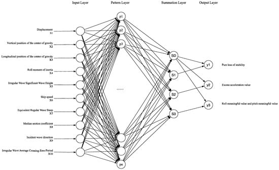
Figure 1.
Architecture of the GRNN-based surrogate model.
(1) Input layer. Receive data from learning samples and the number of neurons is equal to the dimension of the input vector, that is, X1, X2…, X10.
(2) Pattern layer. Calculate the value of the Gaussian function for each sample in the training and test samples. The number of neurons in the pattern layer equals the number of training samples. The transfer function of the neurons in the pattern layer is
In the formula, X is the network input vector, Xi is the training sample vector corresponding to the input neuron, and σ is the hyperparameter of the GRNN.
(3) Summation layer. Two types of summing neurons are utilized for summing. One type performs an arithmetic summation of the outputs from all neurons in the pattern layer, where the connection weights between the pattern layer and these neurons are set to 1, and the transfer function is
The other type of summation calculates the weighted summation of all pattern layer neurons, and weighting coefficient is the j-th element of the label of the training sample corresponding to the j-th pattern layer node, and the transfer function is
(4) Output layer. The output layer corresponds to the ship’s dynamic stability performance, such as the GZ curve value in the wave in the PL mode, the acceleration value in the EA mode, and the roll amplitude in the PR mode. These values have the ratio of the two types of node values in the summation layer, namely
A GRNN can be regarded as a kernel regression model, in which each training sample defines a radial basis function. The smoothing parameter governs the bias–variance trade-off. Unlike conventional neural networks, training does not require backpropagation; it only involves storing the samples. The inference complexity is O(N), where N is the number of training samples. Such complexity is acceptable for offline pre-computation or after prototype selection. These characteristics make the GRNN an appealing surrogate modeling approach when both accuracy and simplicity are prioritized.
2.2. The Algorithm Flow of the GRNN Ship Dynamic Stability Performance Surrogate Model
The algorithm of the GRNN ship dynamic stability performance forecasting process is shown in Figure 2. And the pseudocode of the algorithm is presented below (Algorithm 1).
| Algorithm 1: GRNN model | |
| Input: | |
| The original data matrix: | |
| The Euclidean distance: ED | |
| The smoothing parameter: | |
| The training data: | |
| The test data: | |
| Output: | |
| GRNN model with determined | |
| 1 | Normalize D. |
| 2 | using K-fold cross-validation |
| 3 | Repeat |
| 4 | For do |
| 5 | Compute |
| 6 | End for |
| 7 | Compute |
| 8 | Compute |
| 9 | based on the value of RMSE and R2, |
| 10 | Until that minimizes the RMSE and maximizes R2 |
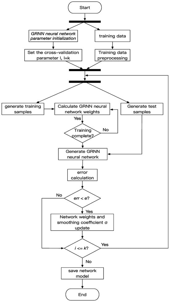
Figure 2.
Algorithmic workflow of the GRNN ship dynamic stability performance surrogate model.
2.3. Verification for the GRNN Ship Dynamic Stability Performance Surrogate Model
To verify the validity of the model, a large container ship is selected. The main dimensions of the ship are shown in Table 1, and its ship type is shown in Figure 3. The dynamic performance characteristic data set (the parameters are shown in Table 2), and the numerical model results of the dynamic stability performance of the ship are directly calculated by the IMO second-generation intact stability criterion calculation function in the calculation software stability module of the COMPASS project developed by the CCS [23,24]. The software has undergone validation through numerical simulations and model testing, and has been utilized by the Chinese delegation for their research in developing the second-generation intact stability criteria in collaboration with the IMO.

Table 1.
Parameters of a large container ship [7].
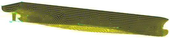
Figure 3.
Meshes used by the simplified method for 10,000-TEU container ship (S25) [7].
Table 2.
The dynamic performance characteristic data set.
The verification of the validity of the GRNN model takes the following steps:
- (1)
- (2)
- Randomly select one working condition from the remaining working conditions in the data set for prediction.
- (3)
- Compare and analyze the accuracy of the prediction results and the calculation results of the numerical model.
Table 3.
Model Training/Testing Parameters.
Table 3.
Model Training/Testing Parameters.
| Ship Dynamic Stability Model | Number of Training Data (Piece)/Working Conditions | Number of Testing Data (Piece)/Working Conditions |
|---|---|---|
| EA | 13,158/44 | 306/1 |
| PL | 20,000/21 | 1000/1 |
| PR | 111,384/29 | 3978/1 |
The working conditions in Table 2 were randomly split into training and testing sets; Table 3 summarizes the split.
To accurately measure the prediction accuracy of the prediction model, this paper uses the root mean square error (RMSE) and the coefficient of determination (R2) to compare the prediction results. It is defined as follows.
where T represents the number of output data; is the true value of ship dynamic stability; is the predicted value of ship dynamic stability; is the average value of .
Table 4 reports the prediction accuracy of the GRNN dynamic stability surrogate model for eight randomly selected working conditions. The results demonstrate good agreement with the numerical simulation outcomes, with the average R2 values reaching 0.996, 0.998, and 0.999 for EA, PL, and PR, respectively. This indicates that the GRNN surrogate can effectively approximate the numerical model. In terms of accuracy, the method achieves high precision for EA and PL, with root mean square errors of about 0.02 and 0.04, respectively. However, there is a notable deviation in the prediction of PR, where the maximum root mean square error reaches 0.2 and the average value is around 0.08, indicating that further refinement is required to ensure reliability in practical applications.
Table 4.
Prediction accuracy of GRNN ship dynamic stability performance prediction model.
Complementing the accuracy analysis, Table 5 presents the training and inference times of the GRNN surrogate model for the three stability failure modes across eight randomly selected working conditions. Experiments were performed on a workstation with Intel Core i7-14700HX CPU, 48 GB RAM and NVIDIA GeForce RTX 4070 GPU. The results show that the average one-time training costs for EA, PL, and PR are 3.371, 38.162, and 629.117 s, respectively. The corresponding average inference times per condition are 0.336, 0.852, and 2.245 s. Compared with the median runtime of the COMPASS solver under comparable conditions, the GRNN surrogate achieves several orders of magnitude reduction in computational cost. These findings highlight that, once trained, the surrogate model can rapidly evaluate new loading and sea state conditions with negligible additional burden, thereby providing strong support for large-scale and near real-time stability assessment.
Table 5.
Computational cost of GRNN ship dynamic stability performance prediction model.
It should be emphasized that the input features used in this study already explicitly incorporate parameters closely related to the ship’s geometrical characteristics, such as displacement, longitudinal and vertical centers of gravity (LCG, VCG), roll moment of inertia (RMI), and midship section coefficient. These quantities are determined by the hull geometry and appendage configuration and play essential roles in dynamic stability behavior. For example, displacement and center-of-gravity positions directly influence buoyancy distribution and trim, while the roll moment of inertia strongly affects the amplitude and period of roll response. Therefore, the dataset effectively captures the geometric attributes of the vessel through its feature representation.
3. An Improved Ship Dynamic Stability Performance Surrogate Model Based on K-Means and GRNN Hybrid Neural Network
The previous experiments indicate that, except for the large mean square error of the PR prediction results, the results of the GRNN ship dynamic stability performance surrogate model are comparable to those based on hydrodynamics under the same type of loading conditions, navigation, and environmental conditions of the ship in waves. The calculation results of the method numerical simulation have a good fit.
However, during actual ship operations, loading, navigation, and environmental conditions vary continuously, and the hydrodynamic characteristics of the same vessel change accordingly. Figure 4 shows the distribution of the center-of-gravity coordinates across the 49 working conditions considered in the experiments, where variations in the center of gravity is closely related to buoyancy and thus affects the trim. It also illustrates that the loading conditions—particularly displacement and center-of-gravity position—exhibit clear clustering patterns.
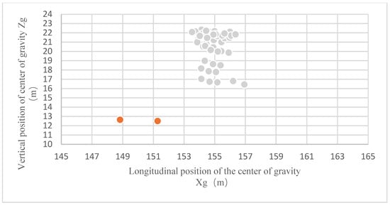
Figure 4.
Scatter diagram of ship center of gravity in different working conditions.
The GRNN is a kernel-based model in which each training sample corresponds to a radial basis function. Consequently, the predictive behavior of GRNN is highly sensitive to the spatial distribution of training samples: inference is essentially performed as a normalized weighted average over all stored patterns, and the relative contribution of each sample depends on its kernel similarity to the query point. When the input space exhibits heterogeneous sub-regions, a single global GRNN may struggle to capture cross-cluster nonlinearities.
In the context of ship dynamic stability, the observed clustered patterns in loading conditions (Figure 4) can be interpreted as arising from underlying physical characteristics such as displacement, center of gravity, and roll inertia. These physical drivers induce a natural clustering structure in the stability responses.
Hypothesis 1.
Clustering the input space and training cluster-specific GRNNs is expected to significantly improve prediction accuracy compared with a single global GRNN.
To verify the proposed hypothesis, K-means clustering is employed to partition the input feature space into K relatively homogeneous subsets, followed by the independent training of GRNN models within each subset, as illustrated in Figure 5. Prior to model comparison, candidate values of K are preliminarily examined, and clustering quality is assessed using the within-cluster sum of squared errors (SSE). The optimal number of clusters is then determined according to the elbow criterion, while the specific analysis of the SSE–K relationship is presented in the experimental section.
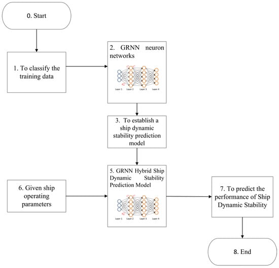
Figure 5.
Flow chart of ship stability performance prediction based on K-means and GRNN hybrid neural network.
The integration of clustering into the surrogate modeling framework is motivated by the fact that classification of training data according to intrinsic characteristics may improve the accuracy of machine learning algorithms. Therefore, a GRNN ship dynamic stability surrogate model hybridized with the K-means method is proposed to enhance the basic GRNN framework. The K-means algorithm is one of the most widely adopted clustering techniques due to its favorable trade-off between accuracy and computational simplicity. Its fundamental principle is to iteratively assign each sample to the nearest cluster center, update the centroid of each cluster as the mean of its assigned samples, and repeat this process until convergence. With advantages such as strong clustering performance, ease of implementation, and computational efficiency, K-means is chosen to classify the ship loading data, effectively partitioning the training samples by loading parameters. Once the training data are classified, independent GRNNs are trained within each cluster under a unified protocol (cluster-wise cross-validation) for feature usage and parameter tuning. A global GRNN trained on all samples is used as a baseline. Finally, predictive performance is evaluated on a held-out test set, with RMSE and R2 reported for EA, PL, and PR. The algorithmic workflow is summarized in Figure 5.
4. Verifications for the Improved Surrogate Model
To analyze the impact of feature classification and preprocessing on the ship dynamic stability performance surrogate model, this paper will combine the ship dynamic stability performance surrogate model based on K-means and GRNN hybrid neural network and the ship dynamic stability performance surrogate model of GRNN neural network model methods for comparison.
The object of the test is still the large container ship shown in Figure 2, and the test parameters are the same as those in Table 1, Table 2 and Table 3.
4.1. Selection of K Value
In the K-means algorithm, the selection of the K value directly affects the clustering results. When the K value is too low, the closest sample points will be correspondingly reduced, and when the selection of the sample points is biased, it may lead to large errors in ship stability prediction; if the value of K is too large, it is easier to introduce many samples with large differences in loading conditions, which will also lead to an increase in the error of ship dynamic stability prediction. Here, the Sum of the Squared Error (SSE) method is used to determine the optimal K value. The error sum of squares is defined as follows.
where is the centroid of cluster .
Figure 6 shows the effect of k on the within-cluster error variance. It can be found that an inflection point appears when k = 3, indicating that a k value of 3 is a good choice. Therefore, the K value in the K-means algorithm in this paper is 3, that is, the training sample data set is divided into 3 clusters.
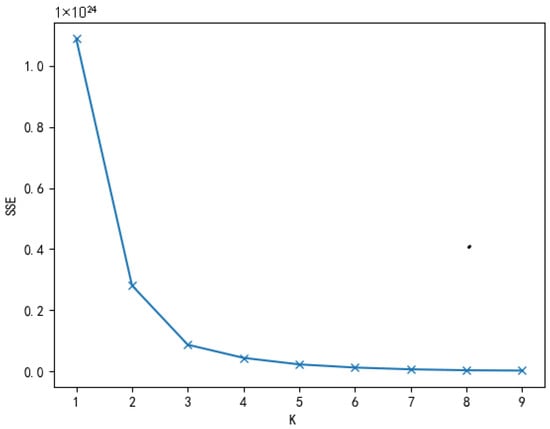
Figure 6.
Relationship between the SSE value and the K value.
4.2. Analysis of Training Data Classification Results
Classifying the input training data set can obtain the training data set of ship dynamic stability stratification, as shown in Table 6, Table 7 and Table 8. It can be seen from the results that (1) the classification of EA is affected by displacement. For example, the displacement of the first category is between 75,000 tons and 95,000 tons, the displacement of the second category is between 146,000 tons and 161,000 tons, and the displacement of the third category is between 140,000 tons and 141,000 tons. (2) In the PL classification, it is mainly affected by the heel angle, followed by the GZ value. For example, the heel angle between 60 and 80 is mainly distributed in the second category. When the heel angle is between 10 and 50, the data are mainly distributed in the first and third categories, the distribution of the smaller GZ value is in the first category, and the distribution of the larger GZ value is in the third category. (3) In the classification of rolling parameters, roll moment of inertia influences the clustering of roll-related samples. The larger roll moment of inertia is classified into the first category, and the smallest roll moment of inertia is classified into the third category.
Table 6.
Clustering results of EA training data.
Table 7.
Clustering results of pure stability loss training data.
Table 8.
Clustering results of PR training data.
4.3. Comparison and Analysis of Ship Dynamic Stability Results
For EA, the comparison results are based on a working condition, 1 wave direction, 1 ship speed, 17 significant wave heights in irregular seas, and 18 irregular wave average zero-crossing periods. The results Including the meaningful value of lateral acceleration, the total number of calculation examples is 306. Eight working conditions were randomly selected, and the results of their EA are shown in Table 9. For the PL, the comparison results are based on a working condition, 1 wave direction, 1 equivalent regular wave wavelength, and 10 equivalent regular wave steepness. The results include the GZ in the wave Curve value, the total number of calculation instances is 1000. The comparison results of pure stability loss are shown in Table 10. For PR, the comparison results are based on a parameter combination example of a working condition, 13 ship speeds, 2 wave directions, 17 significant wave heights in irregular seas, and 18 irregular wave average zero-crossing periods. The results include PR amplitude, and the total number of calculation examples is 3978. The comparison results of rolling amplitude are shown in Table 11. It can be seen from the results in Table 9, Table 10 and Table 11 that, compared with the GRNN neural network method, the mixed neural network method based on K-means and GRNN is superior to the basic GRNN method in terms of root mean square error and determination coefficient of the results. The experimental results are consistent with the above hypothesis, that is, the ship dynamic stability performance data will be affected by its physical characteristics and exhibit clustering patterns.
Table 9.
Comparison of EA result errors.
Table 10.
Comparison of PL result errors.
Table 11.
Comparison of PR result errors.
For completeness, the computational cost of K-means + GRNN is reported in Table 12. The results indicate that the effect of clustering on training time is mode-dependent. For EA and PL, the clustered models achieve shorter training times than the global GRNN, because the relatively small datasets are partitioned into even smaller subsets, thereby reducing the burden of each GRNN and improving GPU utilization. In contrast, for PR, which involves a larger and more complex dataset, training time becomes longer, as splitting into clusters still results in sizable subsets and parallelization introduces additional overhead. Despite these variations, the inference time per sample remains comparable between K-means + GRNN and the global GRNN. More importantly, both approaches require only a fraction of the time demanded by traditional numerical simulations, confirming that the proposed method maintains significant efficiency advantages while improving predictive accuracy.
Table 12.
Computational cost of the K-means + GRNN surrogate model.
5. Conclusions
This study explores the application of a neural network approach to develop a surrogate model for assessing ship dynamic stability, aimed at effectively addressing the limitations in efficiency and implementation cost associated with the traditional CFD-based numerical simulation method. In this paper, the method of using a GRNN to construct a surrogate model of ship dynamic stability is studied. The experimental results show that this method can be used to replace the traditional numerical calculation model. In dynamic changes, the accuracy of the model directly trained by the GRNN method will be affected by the training data. It is not enough to use the coefficient of determination (R2) as the basis for measuring the quality of the model. Sometimes the coefficient of determination between the prediction result and the numerical calculation result is even above 0.9, but there are still deviations between the actual prediction results and the numerical results (Figure 7a and Figure 8a) and even a large deviation (Figure 9a). Therefore, it cannot be directly used as a surrogate model for numerical calculation models.
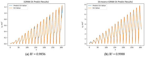
Figure 7.
Comparison of EA Prediction.
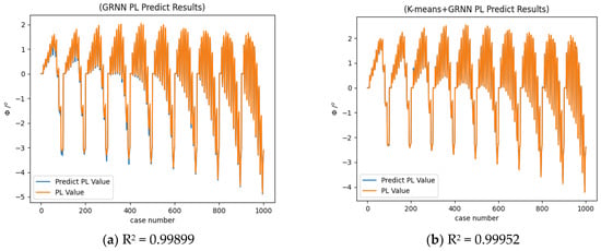
Figure 8.
Comparison of Pure Stability Loss Forecasts.
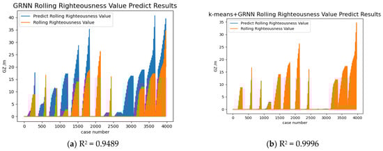
Figure 9.
Comparison of PR Forecast Results.
For this reason, this paper considers the influence of stowage parameters on the dynamic stability of the ship during its actual operation. Based on the GRNN prediction model, the K-means algorithm is used to cluster the input sample data by constructing a hybrid neural network. In this framework, the clustering step does not merely reorder the input data; instead, each cluster of samples is used to train an independent GRNN model, ensuring that the learned relationships are specialized to homogeneous subsets of loading conditions. Through empirical analysis and comparison, the ship dynamic stability performance prediction model can control the variance within 0.05, which basically agrees with the numerical simulation results based on the hydrodynamic method at 98.9%.
In addition, the results on computational cost demonstrate that both GRNN and the K-means + GRNN framework provide significant time efficiency compared with CFD-based simulations, with training and inference times reduced from days or weeks to seconds or minutes. This confirms that the proposed surrogate modeling approach not only improves predictive accuracy through clustering but also retains the computational efficiency necessary for practical engineering applications.
Author Contributions
Conceptualization, J.T.; Methodology, Q.S.; Software, Q.S.; Validation, J.T.; Investigation, Y.Z.; Data curation, Q.S. and Y.Z.; Writing—original draft, Q.S.; Writing—review & editing, J.T. and Y.Z.; Visualization, Q.S., J.T. and Y.Z.; Supervision, Y.Z.; Project administration, Y.Z. All authors have read and agreed to the published version of the manuscript.
Funding
This research received no external funding.
Data Availability Statement
The datasets presented in this article are not readily available because [ship information has not been authorized for publication]. Requests to access the datasets should be directed to [yhzhou@ccs.org.cn].
Conflicts of Interest
The authors declare no conflict of interest.
References
- Gao, N.; Hu, A.; Hou, L.; Chang, X. Real-time ship motion prediction based on adaptive wavelet transform and dynamic neural network. Ocean Eng. 2023, 280, 114466. [Google Scholar] [CrossRef]
- Peters, W.S.; Belenky, V.I. Second Generation Intact Stability Criteria: An Overview. In Proceedings of the SNAME Maritime Convention (SMC 2022), Houston, TX, USA, 27–29 September 2022. [Google Scholar] [CrossRef]
- International Maritime Organization. Interim Guidelines on the Second Generation Intact Stability Criteria; MSC.1/Circ.1627; IMO: London, UK, 2020. [Google Scholar]
- Li, Z.; Ren, H.; Shi, Y. Prediction of wave force based on acceleration potential method. Ship Build. China 2016, 57, 98–108. Available online: https://www.engineeringvillage.com/share/document.url?mid=cpx_M1de782f815a8587305cM619010178163176&database=cpx (accessed on 3 June 2023).
- Yang, B.; Shi, A.-G.; Wang, X.; Wu, M. Simulation of ship’s non-linear roll motion. Chuan Bo Li Xue/J. Ship Mech. 2015, 19, 509–517. [Google Scholar] [CrossRef]
- Li, Z.-F.; Ren, H.-L.; Shi, Y.-Y. Simulation of Ship Motions Based on the HOBEM Acceleration Potential Method. Chuan Bo Li Xue/J. Ship Mech. 2019, 23, 1034–1044. [Google Scholar] [CrossRef]
- Jiao, J.-L.; Sun, S.-Z.; Li, J.-D.; Chen, C.-H. Extrapolation of actual ship responses from large-scale model seakeeping measurement based on system identification. Chuan Bo Li Xue/J. Ship Mech. 2019, 23, 1310–1319. [Google Scholar] [CrossRef]
- Zhou, Y.; Sun, Q.; Shi, X. Experimental and numerical study on the parametric roll of an offshore research vessel with extended low weather deck. Ocean Eng. 2022, 262, 111914. [Google Scholar] [CrossRef]
- Liu, L.; Chen, M.; Wang, X.; Zhang, Z.; Yu, J.; Feng, D. CFD prediction of full-scale ship parametric roll in head wave. Ocean Eng. 2021, 233, 109180. [Google Scholar] [CrossRef]
- Huang, S.; Jiao, J.; Chen, C. CFD prediction of ship seakeeping behavior in bi-directional cross wave compared with in unidirectional regular wave. Appl. Ocean Res. 2021, 10, 102426. [Google Scholar] [CrossRef]
- Kim, D.; Tezdogan, T.; Incecik, A. A high-fidelity CFD-based model for the prediction of ship manoeuvrability in currents. Ocean Eng. 2022, 256, 111492. [Google Scholar] [CrossRef]
- Zhang, L.; Feng, X.; Wang, L.; Gong, B.; Ai, J. A hybrid ship-motion prediction model based on CNN–MRNN and IADPSO. Ocean Eng. 2024, 299, 117428. [Google Scholar] [CrossRef]
- Li, S.; Wang, T.; Li, G.; Skulstad, R.; Zhang, H. Short-term ship roll motion prediction using the encoder–decoder Bi-LSTM with teacher forcing. Ocean Eng. 2024, 295, 116917. [Google Scholar] [CrossRef]
- Li, Z.; Dong, J.; Song, Z.; Zhang, H.; Guo, Y. Prediction of ship roll motion based on combination of phase space reconstruction theory and Elman network. In Proceedings of the 2016 IEEE International Conference on Information and Automation (ICIA), Ningbo, China, 1–3 August 2016; pp. 686–689. [Google Scholar]
- Li, C.; Zhang, W.; Zhou, T.; Ma, S.; Wang, C. Prediction of ship rolling motion based on NARX neural network. In Proceedings of the 2021 33rd Chinese Control and Decision Conference (CCDC), Kunming, China, 22–24 May 2021; pp. 4664–4668. [Google Scholar]
- Peña, F.L.; Gonzalez, M.M.; Casás, V.D.; Duro, R.J. Ship roll motion time series forecasting using neural networks. In Proceedings of the 2011 IEEE International Conference on Computational Intelligence for Measurement Systems and Applications (CIMSA), Ottawa, ON, Canada, 19–21 September 2011; pp. 1–6. [Google Scholar]
- Fu, H.; Gu, Z.; Wang, H.; Wang, Y. Ship motion prediction based on ConvLSTM and XGBoost variable weight combination model. In Proceedings of the OCEANS 2022-Chennai, Chennai, India, 21–24 February 2022; pp. 1–8. [Google Scholar]
- Xu, S.; Gao, Z.; Xue, W. CFD database method for roll response of damaged ship during quasi-steady flooding in beam waves. Appl. Ocean Res. 2022, 126, 103282. [Google Scholar] [CrossRef]
- Bassam, A.M.; Phillips, A.B.; Turnock, S.R.; Wilson, P.A. Artificial neural network based prediction of ship speed under operating conditions for operational optimization. Ocean Eng. 2023, 278, 114613. [Google Scholar] [CrossRef]
- Nie, Z.; Shen, F.; Xu, D.; Li, Q. An EMD-SVR model for short-term prediction of ship motion using mirror symmetry and SVR algorithms to eliminate EMD boundary effect. Ocean Eng. 2020, 217, 107927. [Google Scholar] [CrossRef]
- Sinaga, K.P.; Yang, M.-S. Unsupervised K-means clustering algorithm. IEEE Access 2020, 8, 80716–80727. [Google Scholar] [CrossRef]
- Specht, D.F. A general regression neural network. IEEE Trans. Neural Netw. 1991, 2, 568–576. [Google Scholar] [CrossRef] [PubMed]
- Zhou, Y.-H.; Ma, N.; Shi, X.; Zhang, C. Direct calculation method of roll damping based on three-dimensional CFD approach. J. Hydrodyn. 2015, 27, 176–186. [Google Scholar] [CrossRef]
- Zhou, Y.-H.; Ma, N.; Lu, J.; Gu, M. A study of hybrid prediction method for ship parametric rolling. J. Hydrodyn. 2016, 28, 617–628. [Google Scholar] [CrossRef]
Disclaimer/Publisher’s Note: The statements, opinions and data contained in all publications are solely those of the individual author(s) and contributor(s) and not of MDPI and/or the editor(s). MDPI and/or the editor(s) disclaim responsibility for any injury to people or property resulting from any ideas, methods, instructions or products referred to in the content. |
© 2025 by the authors. Licensee MDPI, Basel, Switzerland. This article is an open access article distributed under the terms and conditions of the Creative Commons Attribution (CC BY) license (https://creativecommons.org/licenses/by/4.0/).