Article

Energy Minimization for Underwater Multipath Time-Delay Estimation

by
Miao Feng
1,*,
Shiliang Fang
1,*,
Liang An
1,
Chuanqi Zhu
1,
Shuxia Huang
2,
Qing Fan
1 and
Yifan Zhou
1
1
Key Laboratory of Underwater Acoustic Signal Processing, Ministry of Education, Southeast University, Nanjing 210096, China
2
Nanjing Research Institute of Electronic Engineering, Nanjing 210000, China
*
Authors to whom correspondence should be addressed.
J. Mar. Sci. Eng. 2025, 13(9), 1764; https://doi.org/10.3390/jmse13091764
Submission received: 10 August 2025 / Revised: 8 September 2025 / Accepted: 11 September 2025 / Published: 12 September 2025
(This article belongs to the Section Ocean Engineering)

Abstract

To address the multipath delay estimation problem in distributed hydrophone passive localization systems, a global energy minimization-based method is proposed in this paper. In this method, correlation pulses are treated as tracking targets, and their trajectories are estimated from correlograms formed by multiple frames. Specifically, an energy function is designed to jointly encode pulse similarity, motion continuity, trajectory persistence, data fidelity, and regularization, thereby reformulating multipath delay estimation as a global optimization problem. In order to balance the discreteness of observations and the continuity of trajectories, the optimization process is implemented alternating between discrete association (solved via α -expansion) and continuous trajectory fitting (using weighted cubic splines). Furthermore, a dynamic hypothesis space expansion strategy based on trajectory merging and splitting is introduced to improve robustness while accelerating convergence. By exploiting both the intrinsic characteristics of correlation pulses in multi-frame processing and the physical properties of motion trajectories, the proposed method achieves higher tracking accuracy without requiring prior knowledge of the number of delay trajectories in a noisy environment. Numerical simulations under various noise conditions and sea trial results validate the superiorities of the proposed multipath delay estimation method.

1. Introduction

The utilization of acoustic multipath delay for detection and localization has broad applications in fields such as geological exploration, industry, and communication [1,2,3,4,5,6,7]. Multipath propagation occurs when acoustic waves reflect, refract, or scatter upon encountering different interfaces within the propagation medium. These distinct propagation paths provide valuable insights into the internal structural details of the medium. Multipath delay refers to the differences in signal arrival times at receivers due to multipath propagation. Estimating this delay helps obtain a more comprehensive understanding of the propagation medium, facilitates target identification, and improves the accuracy of target localization.
In oceanic environments, multipath effects are typically caused by surface reflections, seabed reflections, or a combination of both. Current research on oceanic multipath phenomena mainly focuses on two areas. The first is channel estimation, which involves estimating delays, Doppler shifts, and the signal attenuation of different paths using cooperative signals, primarily to enhance the quality of underwater acoustic communications [8,9,10,11]. The second is source localization, where multipath delays are analyzed to extract the source’s arrival pattern. By incorporating these delays into acoustic propagation models and leveraging known oceanic environmental parameters, the location of the sound source can be estimated accordingly [12,13,14,15,16]. Depending on the specific application scenario, these delays can refer to those caused solely by multipath effects on a single hydrophone or more complex delays resulting from the combined influence of multipath effects and the spatial position of multiple hydrophones. In either case, accurate delay estimation is crucial, as it directly impacts the precision of subsequent source localization.
Zhang et al. [14] characterized the estimation of multipath delay as a medium-resolution time-delay estimation problem in the absence of prior information, considering its range from a few milliseconds to several tens of milliseconds. A comparison of existing delay estimation algorithms was provided in terms of resolution, computational complexity, signal-to-noise ratio (SNR) requirements, and the need for prior information. For broadband impulsive acoustic sources, Tiemann et al. [17] directly extracted six arrival delays of impulsive “clicks” made by sperm whales from the normalized spectral sum time series (available frequency: 2000–6600 Hz; length: approximately 20 ms). However, for broadband continuous sources, multipath arrivals overlap in time, making it infeasible to separate them directly from time sequences. The generalized cross-correlation (GCC) algorithm, which can aggregate and compress the energy of broadband noise into a single pulse, simplifies the situation. Conventional methods based on GCC, such as peak amplitude detection (CPAD) in cross-correlation function, are highly susceptible to noise. To address this issue, many researchers have exploited the evolutionary characteristics of multipath delays in either the temporal or spatial domain to achieve more robust time-delay estimation and tracking under noisy conditions [18]. These characteristics are specifically reflected in the cross-correlation function as the systematic movement of peaks (representing true delays) over time or space. In the spatial domain, the delay-and-sum (DAS) method based on a vertical line array was proposed to estimate multipath delays of an explosive source in a reliable acoustic path (RAP) environment by leveraging the spatial accumulation effect [19]. Michalopoulou and Jain [20] applied particle filtering (PF) to extract the arrival times and amplitudes of different multipath signals at spatially separated receivers. In the temporal domain, Woolfe et al. [21] extracted coherent arrivals from ambient noise correlations by aligning and averaging them within short time windows. By vertically stacking cross-correlation functions to form a correlogram, multipath delays appear as striation lines. Gebbie et al. [22] manually extracted these streaks using point selection and linear interpolation to ensure accuracy. Later, they improved the system by automating the processing of correlation diagrams using a particle filter [23]. However, this method approximates the correlation pulse using a Gaussian function, and any mismatch between the actual pulse shape and the model may degrade system performance. To address uncertainties in pulse shapes, Duan et al. [24] developed a state-space method that tracks the evolution of peak points in the cross-correlation function by PF. Feng et al. [25], modeled delay variations with a hidden Markov model (HMM), and employed the Viterbi algorithm to extract delay trajectories. However, the aforementioned methods assume either a single source or a predefined number of delay trajectories, making them unsuitable for automatically tracking when the number of sources and time delay trajectories is unknown.
This study aims to extract multiple time delay trajectories using a correlogram under the condition that the number of trajectories is unknown. Ideally, the true time delays in the cross-correlation function correspond to high-amplitude correlation peaks. When the cross-correlation function is vertically stacked in chronological order, each correlation peak forms a distinct continuous trajectory, with its evolution determined by the motion characteristics of the sound source and the receiving point. If these correlation peaks are regarded as targets to be identified and tracked, the problem of multipath time-delay estimation can be interpreted as a multi-target tracking problem. Inspired by multi-object tracking in the visual domain [26,27,28], this paper proposes a global energy minimization-based method for multipath delay estimation. This method assigns an energy value to each candidate solution through an energy function and multi-target tracking is achieved by optimizing the energy function. The energy function consists of multiple cost terms, each of which characterizes the plausibility of candidate solutions based on the naturally evolving physical properties of the system. The total energy is computed as a linear superposition of these cost terms. The optimization process primarily involves target association in the discrete domain and trajectory estimation in the continuous domain. By alternately implementing these two steps, the method iteratively refines the solution until energy minimization is obtained.
The remainder of the article is organized as follows: Section 2 introduces the correlation function modeling for multipath propagation. Section 3 establishes an energy function and proposes an effective multipath time-delay estimation method based on energy minimization. Section 4 conducts simulation experiments to evaluate the proposed method, and verifies it through sea trial data. Finally, the conclusions are reached in Section 5.

2. Correlation Function Modeling for Multipath Propagation

The ocean acoustic channel is a highly complex medium composed of the ocean and its boundaries. Its internal structure, along with the distinct characteristics of the upper and lower surfaces, significantly influences sound wave propagation. Various phenomena, including multipath effects, Doppler shifts, and fluctuation effects, cause deviations in signal amplitude, frequency, and propagation time at the receiver compared to the original source signal. Among these, multipath effects encompass both single-reflection paths, which result from reflections off the seabed or sea surface, and multiple-reflection paths arising from the combined interactions of both boundaries. Assuming that the propagation has anegligible influence on the signal frequency and that multipath signals can be captured within a continuous time window, the discrete signal received by the hydrophone can be modeled as a linear superposition of multipath components.
r i ( n ) = k = 1 K α i , k s ( n τ i , k ) + w i ( n ) ,
where s ( n ) represents the source signal, modeled as a time-continuous broadband signal in this study. α i , k and τ i , k denote the amplitude attenuation factor and time delay of the signal associated with the k propagation path between the ith hydrophone and the sound source, respectively. w i ( n ) represents the uncorrelated additive noise at the ith hydrophone.
The cross-correlation of the signals received by two distinct hydrophones is given by
R i , j ( τ ) = E r i ( n + τ ) r j ( n ) = E k = 1 K α i , k s ( n τ i , k + τ ) + w i ( n + τ ) l = 1 L α j , l s ( n τ j , l ) + w j ( n ) = k = 1 K l = 1 L α i , k α j , l R s s ( τ τ i , k + τ j , l ) + k = 1 K R s w ( τ τ i , k ) + l = 1 L R w s ( τ + τ j , l ) + R w w ( τ τ i , k + τ j , l ) ,
where R s s denotes the autocorrelation of the source signal. For finite broadband signals, the autocorrelation typically exhibits a distinct pulse near the origin, with its exact shape varying slightly depending on the characteristics of the source [24]. The first term in Equation (2) represents the sum of the cross-correlations of signals arriving via all propagation paths between the two hydrophones, while the last three terms correspond to the cross-correlation between noise and signal, as well as the autocorrelation of noise.
Let
R k l ( τ ) = α i , k α j , l R s s ( τ τ i , k + τ j , l ) ,
R s s w w ( τ ) = k = 1 K R s w ( τ τ i , k ) + l = 1 L R w s ( τ + τ j , l ) + R w w ( τ τ i , k + τ j , l ) ,
thus, Equation (2) can be rewritten as
R i , j ( τ ) = k = 1 K l = 1 L R k l ( τ ) + R s s w w ( τ ) .
It can be observed that the cross-correlation function consists of the superposition of R s s components with different amplitude attenuations and time delays, along with the interference of random noise. When considering the effects of propagation paths on amplitude attenuation and signal frequency—such as frequency-selective fading, frequency shifts, and frequency spreading—the shapes of the cross-correlation pulse corresponding to different paths may experience varying degrees of distortion, including time extension and amplitude attenuation. As a result, these pulses cannot be regarded as perfect replicas of an autocorrelation pulse of the source signal. However, within short time intervals where the channel remains approximately stable, the cross-correlation pulses associated with the same path exhibit strong similarity across different time slices, as illustrated in Figure 1, in which each row represents the cross-correlation function within a time interval, and the parameter varying along the vertical axis indicates the index of the time frame. The pulses enclosed by the red dashed line in the middle are the cross-correlation pulses formed by the direct arrivals, and the left and right sides represent the cross-correlation pulses formed by the direct arrivals at one hydrophone and the multipath arrival at the other hydrophone.
It should be emphasized that, although both the channel and noise in underwater acoustics are inherently nonstationary, our formulation assumes them to be locally stationary within short observation windows. This assumption is adopted for mathematical tractability and is commonly used in underwater acoustics [29,30,31,32], while extending the model to nonstationary cases remains an important direction for future work.
The objective of this study is to accurately determine the true positions of correlation pulses in the cross-correlation waveform. Treating the correlation pulses as the target to be identified, multipath delay estimation can be framed as a process of associating and tracking these targets. In this study, we leverage the shape similarity between pulses to associate those generated by the same paths within the time sequence. A key advantage of this approach is that, even if the exact form of the source signal and the theoretical shape of its autocorrelation function are unknown, the similarity of the pulses across different time slices can still contribute to target association.

3. Multipath Time-Delay Estimation

In this section, we propose an energy minimization-based method for multipath delay trajectory estimation. The core idea is to define an energy function that assigns a corresponding value to each potential estimate and then identify the state with the lowest energy. Thus, the multi-object trajectory estimation problem is reformulated as an energy optimization problem. This section is structured as follows: Section 3.1 provides a formalized description of the problem and defines the energy function. Section 3.2 presents a detailed explanation of the individual components of the energy function. Section 3.3 discusses the optimization strategy and the implementation details of the proposed method.

3.1. Problem Statement

Let X = { x i t } represent a set of observed objects, where each observation corresponds to a complete pulse and can be extracted from the cross-correlation function (see Appendix A for details). It should be noted that the correlation pulses formed by multipath propagation may be negative; therefore, negative pulses must also be considered. Each observation is defined as x i t = ( s i t , τ i t , p i t , w i t ) , where s i t denotes the pulse polarity, τ i t represents the time delay at the peak, p i t is the amplitude vector comprising all samples of the pulse waveform, and w i t is the confidence weight (see Appendix A). The superscript t indicates time, where t = 1 , 2 , , T , with T being the total number of frames. The subscript i denotes the index of the observation, where i = 1 , 2 , , I t , and I t is the total number of observed objects in the tth frame.
A set of potential target trajectories is denoted as T = { T 1 , T 2 , , T N } , where N is the number of possible targets which is the number of delay trajectories. The set of observations associated with a given trajectory T n is denoted as D n , where D n = { x i t | x i t T n } , and the total number of observations in T n is represented by C n . The start and end time of trajectory T n are denoted as s n and e n , respectively. Each observation is either assigned to a target trajectory or considered an outlier (denoted as ⌀). For clarity, the notation used in this paper is summarized in Table 1.
Since a target trajectory T n represents a continuous path over time, it is fitted using the parameters of the associated observations D n . Therefore, the first step is to determine which observations correspond to which trajectories, a process referred to as data association. Owing to the smoothness and continuity of cubic spline curves, they are considered well-suited for capturing the true trends in the data while reducing the misclassification caused by noise. Consequently, after data association, we employ weighted cubic spline fitting to model each target trajectory.
For a given candidate estimation result, the energy function is defined as a linear superposition of multiple cost terms:
E = E s i m + E d a t a + E d y n + E p e r + E f i d + E r e g ,
where E s i m quantifies pulse similarity, and E d a t a measures the accuracy of trajectory fitting. The terms E d y n , E p e r , and E f i d account for constraints on trajectory dynamics, length, and the maximum allowable gap between observations, respectively, to ensure physically plausible motion. The regularization term E r e g is introduced to prevent overfitting. Once the energy function is defined, the multipath delay tracking problem reduces to finding a set of trajectories that minimize the total energy:
T * = arg min E ( T ) .

3.2. Energy Function

1.
Similarity. Due to channel effects, the cross-correlation pulses from different propagation paths exhibit distinct deformations compared to the autocorrelation pulse of the source signal. However, pulses corresponding to the same propagation path tend to remain similar across different time frames, as illustrated in Figure 1. Specifically, for the same path indices k and l in Equation (5), R k l shows strong similarity in both polarity and shape. This property facilitates the association of cross-correlation pulses originating from the same path. To quantify pulse similarity, we employ the Structural Similarity Index Measure (SSIM), defined as follows:
S S I M ( x i , x j ) = ( 2 μ i μ j + A 1 ) ( 2 σ i j + A 2 ) ( μ i 2 + μ j 2 + A 1 ) ( σ i 2 + σ j 2 + A 2 ) ,
where μ i and μ j are the mean of the amplitude vectors p i and p j , σ i and σ j are their variance, and σ i j denotes the covariance term. A 1 and A 2 are small constants introduced in the SSIM to avoid instability when the denominator approaches zero. The SSIM is computed for every pair of pulses of D n , and their average is used as the overall similarity score. The energy contribution from pulse similarity is defined as follows:
E s i m = n = 1 N 2 i = 1 C n j > i C n S S I M ( i , j ) C n ( C n 1 ) ,
where C n is the total number of D n , as described in Table 1.
2.
Data term. Multipath delays vary with the relative motion of the source and hydrophones. Since the movement of the source is continuous, the corresponding delay trajectories are also continuous. The weighted cubic spline interpolation provides an effective means of fitting these delay trajectories by capturing their natural evolution.
Figure 2 is a schematic diagram of weighted cubic spline fitting. The observed time delays τ n t associated with the n-th trajectory are used to perform trajectory fitting, where the independent variable is the discrete frame index t { s n , , e n } . The fitted trajectory T n is likewise a function of t, and we denote by T n t the fitted value at frame t.
The data term evaluates the accuracy of trajectory fitting by measuring the Euclidean distance between the observations and the estimated trajectory:
E d a t a * = n = 1 N t = s n e n w n t · τ n t T n t 2 ,
where w n t represents the weight assigned to each observation, which is correlated with its peak amplitude. The start time s n and the end time e n correspond to the indices of the first and last observations in trajectory n, respectively. If an observation does not belong to any trajectory, it is classified as an outlier, ⌀, and assigned a constant cost, C . The final formulation of the data term is given by the following equation:
E d a t a = n = 1 N t = s n e n w n t · τ n t T n t 2 + w · C .
The outlier weight w is set to a small constant to ensure numerical stability, and the outlier cost C is set proportional to the average inlier fitting error.
3.
Dynamics. The fitted trajectory reflects the motion characteristics of the target over time and is constrained by real-world physical limitations. The constant velocity model is widely used to describe the motion characteristics of targets because it supports linear paths, thereby reducing target identity switches. However, this approach also limits the flexibility of target motion. In this study, constraints are primarily imposed on the cubic coefficients of the spline, as they directly influence the maximum velocity of the target:
E d y n = λ n = 1 N f n ,
where f n represents the maximum value among the cubic spline coefficients of trajectory T n . λ is a scaling factor that is introduced to balance the contribution of the trajectory smoothness term and the data fidelity term. In our implementation, λ is tuned empirically within the range of [ 0.1 , 1 ] , and the final value is chosen via cross-validation on synthetic data.
4.
Trajectory Persistence. The proposed method imposes no strict requirements on the start or end points of a target trajectory; it does not necessarily need to begin at the first frame or terminate at the last frame. However, longer trajectories are encouraged. Due to the influence of random noise and other strong interferences, correlation pulses may be completely submerged or become indistinguishable at certain moments or over short time intervals, leading to the disappearance of the targets. In such cases, multiple disconnected short trajectories are often formed, which is not conducive to tracking the trajectories. Assigning a higher cost to short trajectories helps reconnect fragmented tracks and prevents unnecessary identity switches. η is used to adjust the importance of trajectory persistence to the energy function, usually taken as a fixed constant (0.5 in our experiments), which reflects encouragement for long trajectories and punishment for short trajectories:
E p e r = η · n = 1 N ( e n s n ) 1 .
5.
High-order data fidelity. Equation (11) defines the requirement for trajectories to approximate the observations as closely as possible. Nevertheless, considering that targets may be intermittently obscured by noise, it is not mandatory for each frame within a trajectory duration to include a corresponding observation. To mitigate potential errors in trajectory fitting and the merging of short tracks, a constraint on the maximum permissible gap between successive observations is imposed:
E p e r = ξ · n = 1 N G n ,
where G n denotes the maximum number of consecutive frames in which no observation is associated with the trajectory T n . The scaling factor ξ is introduced to penalize long gaps and is set as a constant (empirically chosen in the range of [ 0.01 , 0.05 ] ).
6.
Regularization. The individual cost terms comprising the energy function are mutually constrained. For example, reducing the number of trajectories N tends to lower the energy associated with the E d y n , E p e r , and E f i d terms. However, an overly small N may result in many observations being left unassigned and labeled as outliers, thereby increasing the data term energy E d a t a . In practice, without proper constraints on the number of targets, the model tends to generate a large number of short trajectories. To avoid overfitting, a higher penalty should be imposed for introducing additional targets.
E r e g = N .

3.3. Optimization

Minimizing the energy function in Equation (6) is a challenging problem, as it lacks desirable mathematical properties and cannot be directly solved in closed form. However, given a feasible solution, it is possible to verify its optimality within a finite number of computations and refine it accordingly.
In this work, the optimization of the energy function is decomposed into two interleaved steps: data association and trajectory fitting. This design stems from the observation that target association is inherently a discrete problem, while target motion in the physical world is continuous in time. To accurately capture the underlying motion patterns, trajectories must be smooth and temporally continuous. To reconcile these discrete and continuous aspects, an iterative framework is adopted that alternates between association and trajectory fitting, following a strategy that is conceptually similar to the Expectation-Maximization (EM) algorithm. As summarized in Algorithm 1, the procedure begins with an initialization step that assigns preliminary associations to all observations. Based on these associations, trajectory fitting is performed to estimate continuous motion paths. The fitted trajectories are then used to update the observation-to-target associations in a direction that reduces the overall energy. This process repeats—alternating between association updates and trajectory refinement—until convergence to a (local) minimum of the energy function is achieved.
In the association update step, the α -expansion method is widely adopted. Originally proposed by Boykov [33,34] and later extended and improved in subsequent studies [35,36,37], this method has become a standard approach for discrete multi-label optimization. However, it is important to note that α -expansion only guarantees convergence to a strong local minimum, rather than the global optimum. To mitigate this limitation, we expand the hypothesis space after each iteration, as detailed in Section 3.3. In the trajectory fitting step, our goal is to flexibly account for the varying importance of different observations while maintaining trajectory smoothness. To achieve this, we employ weighted cubic spline fitting, in which each observation is assigned a weight that is proportional to the peak amplitude of its corresponding pulse. This allows more reliable observations to exert greater influence on the fitted trajectory, while ensuring the continuity and smoothness of the motion path.
Algorithm 1 Optimization
Input: Initial observation set X = { x i t }
Output: Optimized trajectory set T *
1:
Assign initial data association
2:
repeat
3:
   Update T by performing weighted cubic spline fitting on observations D n
4:
   Update T by hypothesis space expansion
5:
   Update observation-to-trajectory assignments via α -expansion
6:
until energy convergence or maximum number of iterations reached
7:
return T *
  • Initialization Strategy
Observations are selected using a CFAR detection method, where the false alarm probability can be appropriately increased to reduce the risk of missed detections. The false positives resulting from this process can later be treated as outliers during the data association stage. Once the observations are obtained, an initial association is generated using a simple propagation mechanism. The propagation proceeds sequentially across time frames, from past to future, and two observations are considered to belong to the same trajectory if they share the same pulse polarity and exhibit sufficient proximity in Euclidean space. The procedure begins with observations in the first frame and continues until every observation is either assigned to a trajectory set or labeled as an outlier. The initialization process does not assume a fixed number of targets; however, different search orders and parameter settings may lead to variations in the initial hypotheses. In practice, we observe that although such variations may slightly affect the final result, the overall estimation remains consistent and robust.
  • Hypothesis Space Expansion
The expansion of the hypothesis space primarily involves two operations: trajectory merging and trajectory splitting. Merging refers to the attempt to combine two distinct trajectories into a single longer trajectory, while splitting involves dividing a long trajectory at segments where a prolonged absence of observations occurs. After each iteration, every trajectory is evaluated for potential merging or splitting, and the corresponding energy is recomputed. A trajectory update is accepted only if it results in a lower total energy; otherwise, the original trajectory is retained.
  • Computational Complexity
In the proposed method, the optimization of the energy function is decomposed into two parts: alternating data association and trajectory fitting. The major computational cost arises in the data association step, which is solved using the α -expansion algorithm. This algorithm is a graph-cut-based method with polynomial-time complexity and efficient implementations available. Compared with general-purpose optimization methods, α -expansion converges quickly and is well-suited for large-scale discrete labeling problems. Boykov et al. showed that using maximum flow algorithms to solve graph-cut problems has a worst-case time complexity of approximately O ( n 3 ) , whereas in practical applications, the performance is usually close to linear, i.e., O ( n ) [33].
Let T denote the number of frames, and assume that each frame yields at most M c f a r CFAR-detected delay candidates for a given path. The computational cost for processing one trajectory is therefore O ( T M c f a r ) , and the overall complexity becomes O ( T M c f a r N L ) , where N is the number of trajectories and L is the number of iterations. In practice, only a relatively small number of iterations (about 10) is typically sufficient to achieve good optimization results.
In contrast, the computational complexity of the particle filtering (PF) method increases linearly with the number of particles drawn at each step [24]. For M p f particles, the per-step cost is O ( M p f N ) , resulting in a total complexity of O ( T M p f N ) . To maintain robust performance under low-SNR conditions, a large number of particles is generally required, which substantially increases runtime.

4. Results

In this section, we evaluate the performance of the proposed multipath trajectory estimation method using both simulation experiments and sea trial data. Since our approach is based on cross-correlation functions, we first introduce two statistical metrics to facilitate performance evaluation [24]. The percentage of false peak (PFP) is defined as follows:
P F P k l = 1 1 T t = 1 T δ ( τ ˜ k l , t τ k l , t ) ,
where δ is the unit impulse function and T represents the total number of frames in the cross-correlation function. τ ˜ k l , t denotes the time delay corresponding to the highest peak in the cross-correlation function of frame t, and τ k l , t represents the true time delay in the cross-correlation function of frame t. PFP quantifies the extent to which correlation pulses are obscured by background noise.
The peak-to-peak signal-to-ratio (PSNR) is defined as follows:
P S N R k l = 1 T t = 1 T max ( | R k l , t ( τ ) | ) 3 s t d ( R s s w w , t ( τ ) ) τ [ τ m i n , τ m a x ] ,
where s t d ( R s s w w , t ( τ ) ) represents the standard deviation of peak values generated by the background noise in the cross-correlation function of frame t. The numerator corresponds to the peak value of the true correlation pulse. PSNR quantifies the relative strength of the correlation pulse compared to the background noise.
To analyze the estimation accuracy, the root mean square error (RMSE) is adopted for evaluating the estimated results:
R M S E k l = t = 1 T ( τ ^ k l , t τ k l , t ) 2 / T .

4.1. Numerical Simulation

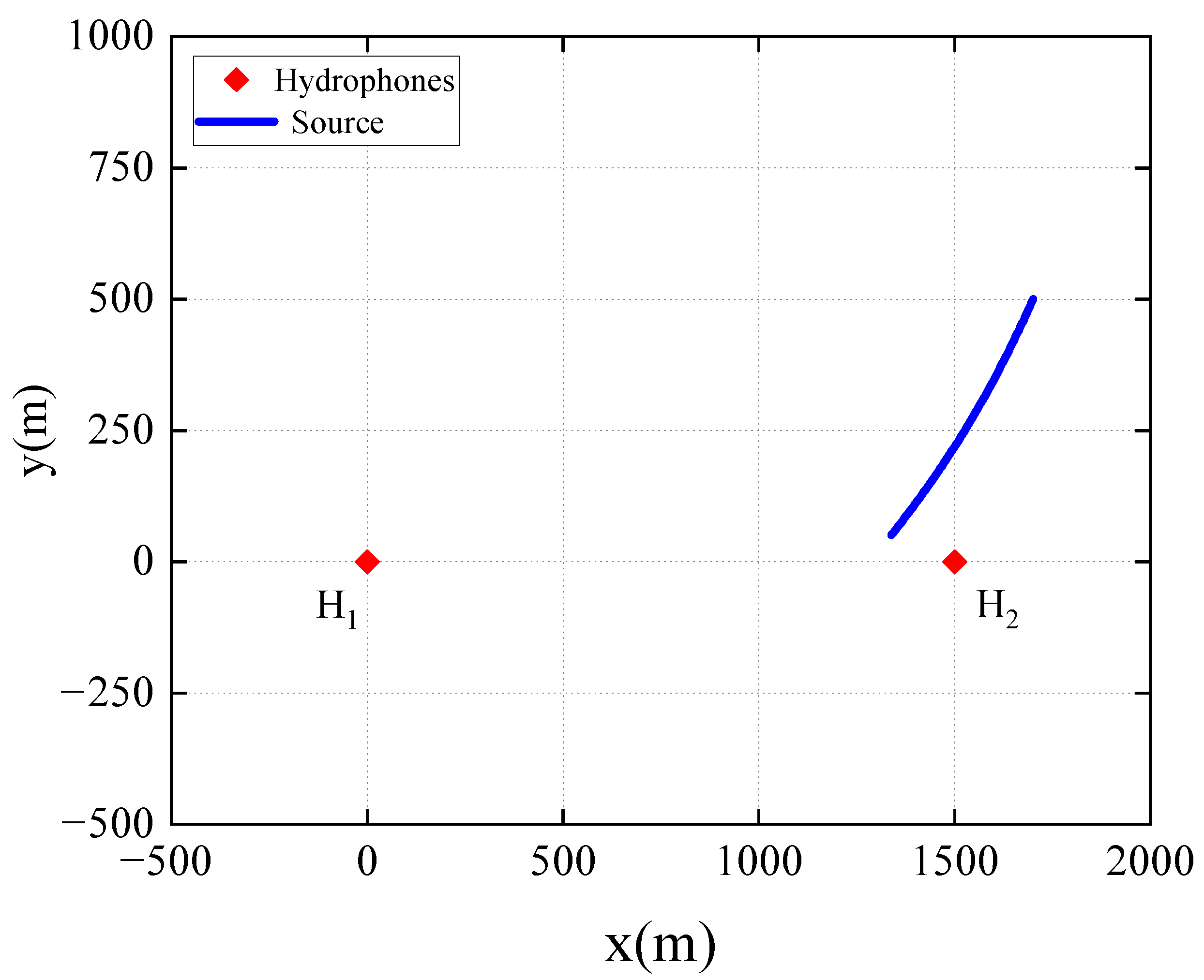
The simulation scenario is illustrated in Figure 3. The two hydrophones are positioned 1.5 km apart, while the sound source moves at a speed of 10 kn, starting from coordinates (1700, 500) and traveling in the negative axis direction. The ocean depth is assumed to be 1000 m. The simulated source signal consists of broadband colored noise, with a total duration of 185 s and a sampling frequency of 20 kHz. Environmental noise is additively introduced into the received signals, and the power of the environmental noise is adjusted to achieve the desired PFP and PSNR values.
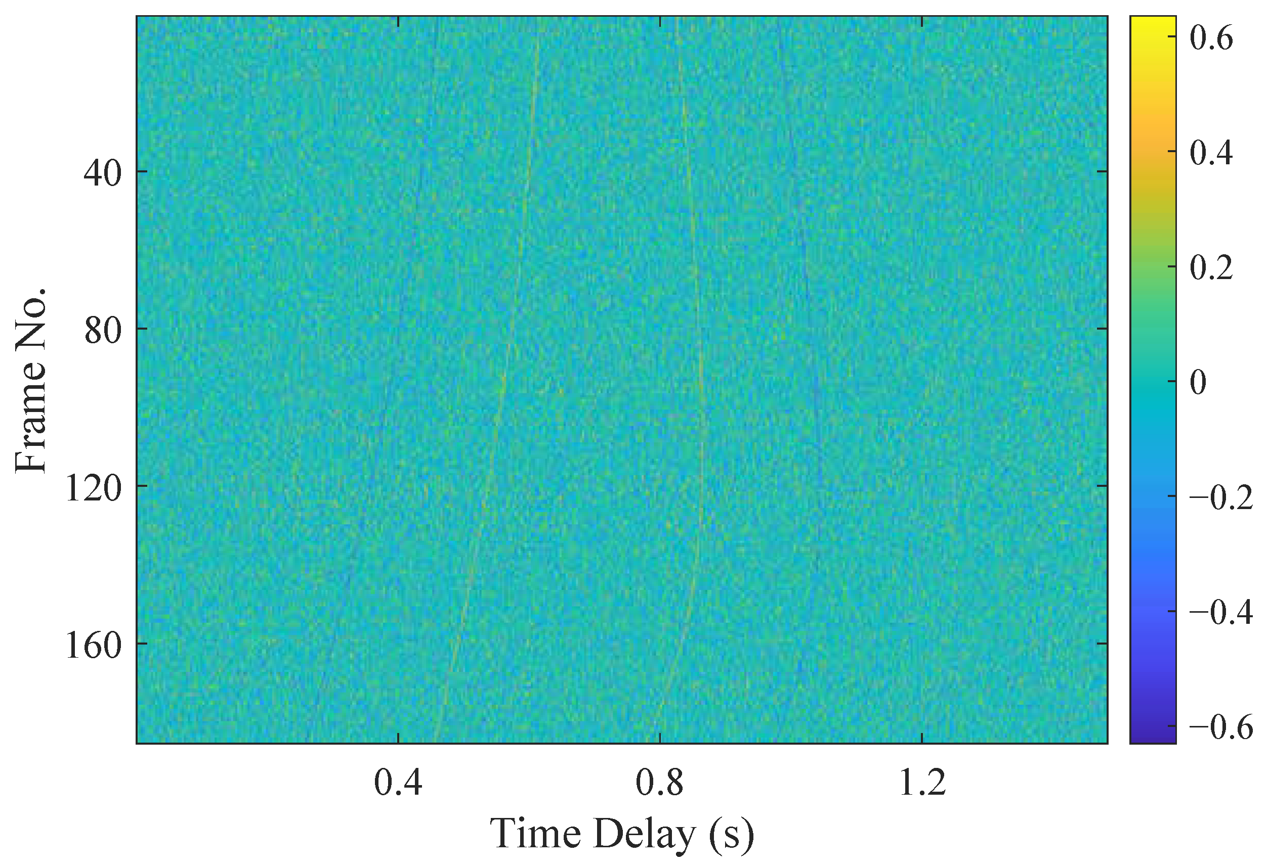
With PFP/PSNR set to 76%/0.84, the correlogram formed by the cross-correlation function of the two hydrophone signals is shown in Figure 4. Four blurred streaks can be observed, indicating that each hydrophone receives one direct path signal and one reflected path signal, resulting in four distinct correlation pulses formed by pairwise combinations. Among them, the correlation pulses formed by the two direct arrivals and the two multipath arrivals are positive pulses, while those formed by the combination of direct and multipath arrivals are negative pulses.
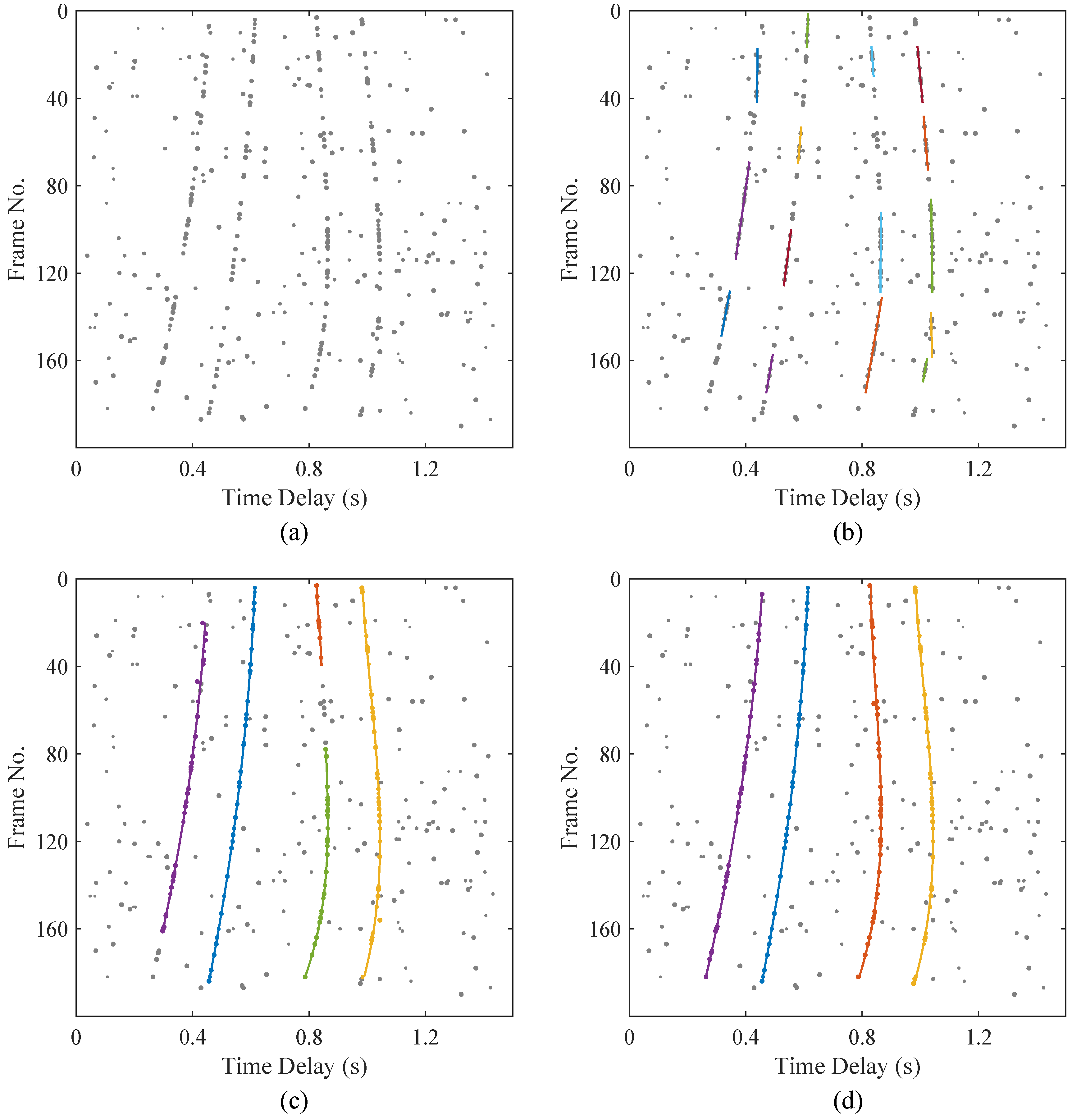
The iterative process of the proposed method is illustrated in Figure 5. Figure 5a shows the set of observations obtained via CFAR detection, where the size of each dot reflects the relative peak amplitude. Figure 5b displays the initial trajectories generated by the initialization strategy, resulting in 15 coarse initial tracks. Figure 5c presents the estimated trajectories after the 6th iteration, and Figure 5d shows the final result after convergence. A detailed comparison from Figure 5b to Figure 5d reveals that the trajectories undergo continuous refinement during the iterative process. These changes include the replacement of observations, trajectory extension, and the merging of adjacent tracks. As the number of iterations increases, the overall energy gradually decreases, and the trajectories converge toward physically plausible paths. After 11 iterations, the algorithm successfully estimates four stable trajectories.
To investigate the influence of different initialization strategies on the final results, several sets of initialization parameters were tested. Figure 6 presents the normalized energy convergence curves under these different configurations. It can be observed that the energy decreases rapidly in the initial iterations and then stabilizes. This is primarily because the initialization phase typically generates a large number of short trajectories, and the removal or merging of these short tracks during the early iterations contributes significantly to the rapid energy reduction. Although different initialization settings may lead to slight variations in the estimated trajectories, their overall impact on final performance is minimal. Alternatively, multiple initialization strategies can be applied in parallel, and the one yielding the lowest final energy can be selected as the final solution.
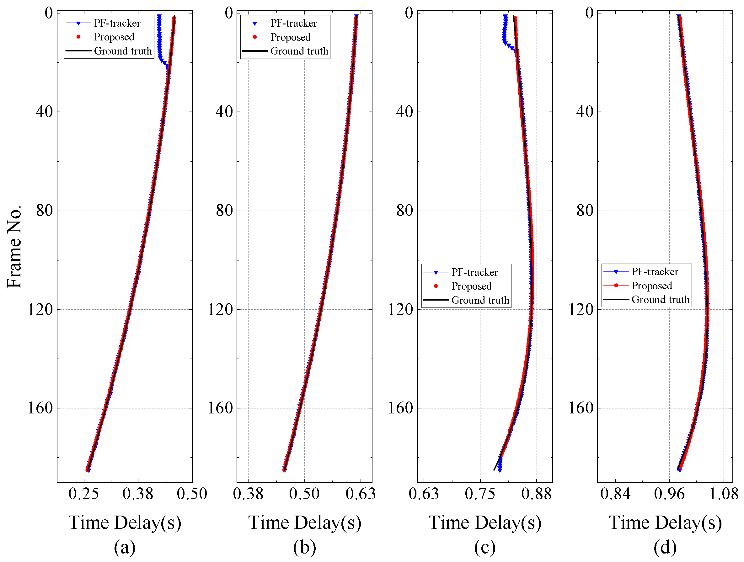
Figure 7 and Figure 8 present the estimation results under different PFP/PSNR conditions using two methods and the ground truth of multiple delay trajectories. Figure 7 and Figure 8 correspond to PFP/PSNR settings of 76%/0.80 and 84%/0.75, respectively. The baseline method used for comparison is a PF-based approach for multipath delay tracking from correlation functions [24]. From the tracking results in Figure 7, both methods successfully estimate all four delay trajectories. However, the PF tracker requires a certain number of frames to lock onto the trajectories in Figure 7a,c—approximately 23 frames and 15 frames, respectively. This delay arises from the nature of particle filtering, in which particles near the true delay have a higher probability of survival, so that the randomness in initialization needs time to converge gradually. This effect is even more pronounced in Figure 8a, where the PF tracker takes about 108 frames to correctly follow the first trajectory. A comparison between Figure 7 and Figure 8 reveals that the proposed method can reconstruct the full delay trajectories in Figure 7. However, in Figure 8, some segments at the beginning or end of the trajectories are missing. This is because, under lower PSNR conditions, the true delay peaks may be obscured by noise and fail to pass the detection threshold. While missing observations in the middle of a trajectory can be inferred and incorporated through the optimization algorithm, those at the start or end are more likely to be missed.
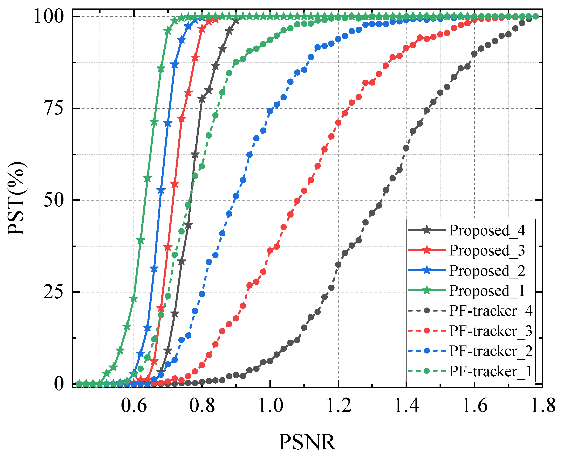
To evaluate the stability and effectiveness of the proposed method, Monte Carlo (MC) simulations were conducted. For each PSNR level, 2000 MC trials were performed, and the tracking performance of each method was quantified using the probability of successful tracking (PST). The PST metric is derived from the RMSE of the estimated trajectories: a trajectory is considered correctly estimated if its RMSE is below a predefined threshold; otherwise, it is classified as a tracking failure. To ensure a more stringent evaluation of algorithm performance, the RMSE threshold was conservatively set to 10 ms in this study.
The simulation configuration is identical to that described in Figure 3, except for the variation in the PSNR. Figure 9 presents the PST for both methods, where four curves are plotted for each method, corresponding to the probability of successfully estimating different numbers of delay trajectories. As expected, achieving reliable estimation of a larger number of trajectories requires increasingly stringent PSNR conditions for both approaches. The proposed method can reliably estimate the trajectories at a minimum PSNR of approximately 0.5, and when the PSNR exceeds 0.9, it can almost perfectly and consistently track all four trajectories. In contrast, the PF-based method exhibits higher sensitivity to noise, requiring a minimum PSNR of about 0.6 to begin producing valid results, and only achieving complete and accurate estimation of all trajectories when the PSNR exceeds 1.8. These results highlight the advantage of the proposed approach in low-to-moderate PSNR regimes, where it maintains a higher probability of correctly estimating multiple trajectories. Overall, under identical PSNR conditions, the proposed method consistently yields better estimation performance compared to the PF-based method, indicating improved robustness in multipath delay tracking.

4.2. Experimental Validation

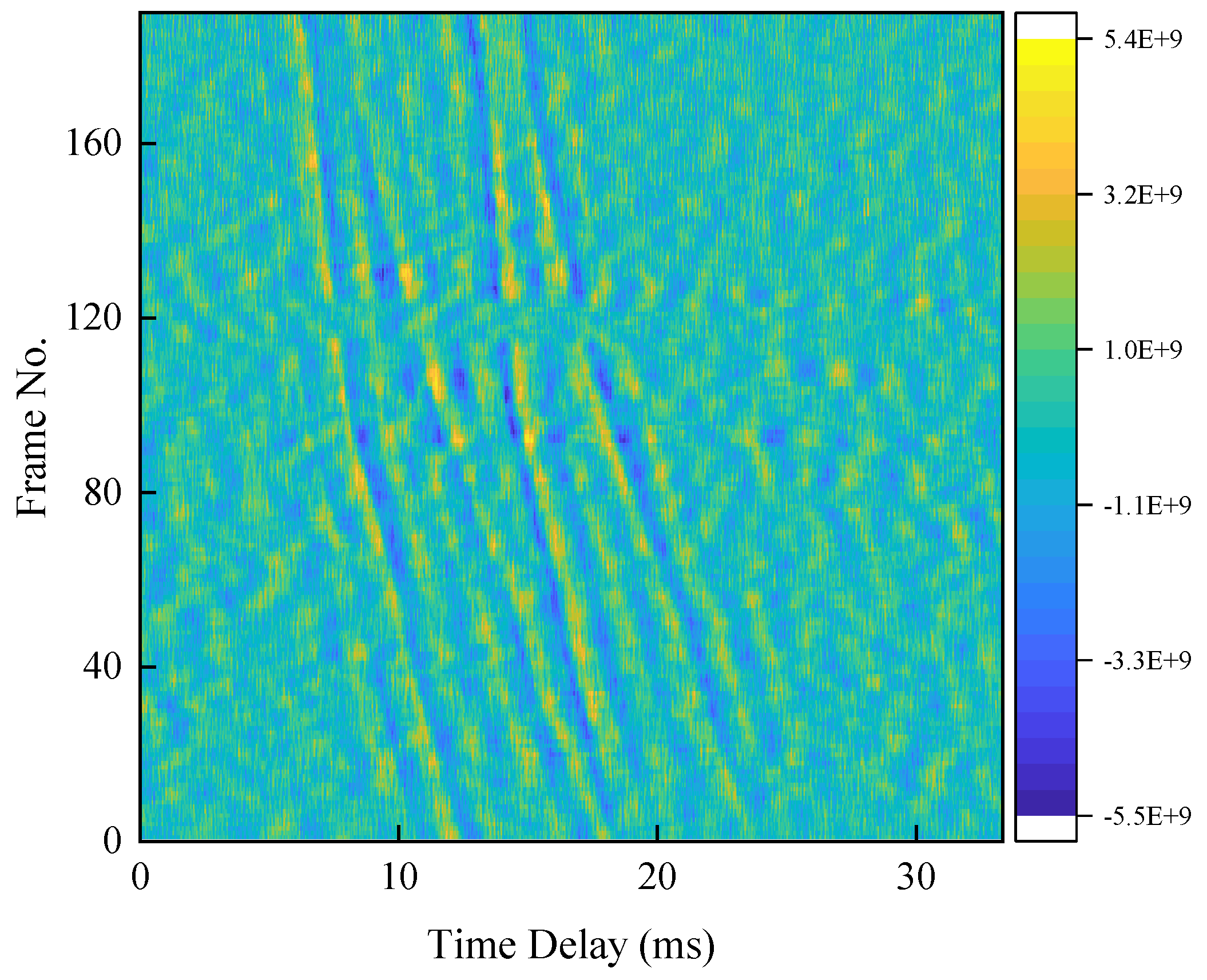
To further validate the proposed method under realistic oceanic conditions, sea trial experiments were conducted in the South China Sea. In this experiment, two omnidirectional hydrophones were deployed at a depth of 20 m, separated by a horizontal distance of approximately 10 km. The acoustic source transmitted a broadband continuous signal, and the system operated at a sampling rate of 50 kHz. The data received by the hydrophones included direct arrival and multipath arrival caused by reflection. Over time, the cross-correlation function between the two hydrophones was computed to form a correlogram, as shown in Figure 10.
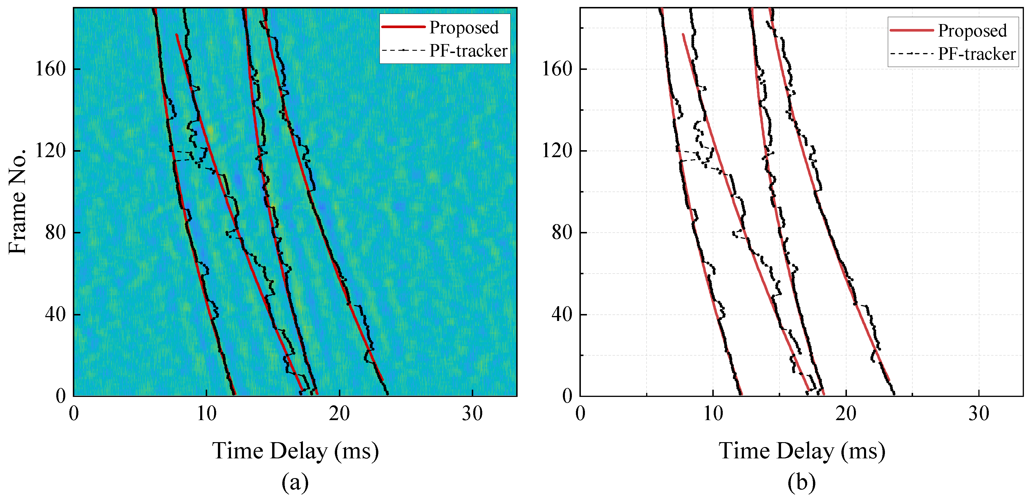
The proposed method was further compared with the PF-based tracking method, and the results are presented in Figure 11. Both methods successfully identified multiple delay trajectories from the real experimental data, indicating their capability to extract multipath structures in complex environments. However, the trajectories estimated by the proposed method appear as four relatively smooth and temporally continuous curves, while the PF tracker exhibits noticeable fluctuations over time. For instance, around frame 120, the PF tracker shows significant oscillations, which are consistent with the interference patterns observed in the correlogram of Figure 10. This instability in the PF tracker can be attributed to particle degeneracy and its sensitivity to local noise peaks in the correlation function, leading to abrupt deviations in the estimated trajectory. In contrast, the proposed method effectively suppresses such disturbances by leveraging the rationality of the trajectorie structure, thereby demonstrating superior stability. In terms of overall performance, the proposed approach exhibits improved temporal continuity and enhanced robustness to noise compared with the PF tracker. Nevertheless, it is not without limitations. For example, although the second trajectory is generally estimated correctly, slight truncations are observed at both ends. This phenomenon is consistent with the findings reported in Section 4.1. In principle, the missing segments could be reconstructed after the main body of the trajectory is estimated using post-processing techniques such as model-based trajectory interpolation or smoothing. However, such reconstruction was deliberately omitted in this study, as it may compromise the adaptability and flexibility of the method in scenarios where the persistence of the target is unknown a priori.

5. Discussion and Conclusions

This paper introduced an energy minimization-based method for underwater multipath time-delay estimation, which integrates discrete data association and continuous trajectory fitting into a unified iterative optimization framework. By leveraging pulse similarity, motion continuity, trajectory persistence, and observation fidelity, the method achieves the robust association and smooth reconstruction of delay trajectories without requiring prior knowledge of the number of paths. The α -expansion strategy ensures efficient association optimization, while weighted spline fitting accounts for varying observation reliability. Moreover, the hypothesis space expansion through trajectory merging and splitting effectively reduces suboptimal convergence and corrects association errors caused by missing or noisy detections. Both numerical simulations and sea trial experiments validated the effectiveness of the proposed method. Compared to particle-filter-based tracking, the proposed approach consistently achieved higher temporal continuity, stronger noise robustness, and more accurate estimation of multipath delay trajectories. Even under challenging low-PSNR conditions, it maintained superior performance in reconstructing complete trajectories. However, the current framework still relies on empirically tuned weight parameters in the energy function, and its present formulation is limited to two-dimensional correlogram analysis. Future research will focus on adaptive parameter selection, more efficient data association algorithms, and extensions to three-dimensional localization. Overall, the proposed method provides a robust and flexible solution for underwater multipath delay estimation and has the potential to significantly improve acoustic source localization and channel characterization in complex ocean environments.

Author Contributions

Conceptualization, M.F. and S.F.; methodology, M.F. and S.F.; software, M.F.; validation, M.F. and S.H.; investigation, M.F., Y.Z. and C.Z.; resources, S.F. and L.A.; writing—original draft preparation, M.F. and Q.F.; writing—review and editing, M.F., S.H. and L.A.; supervision, S.F. and Y.Z.; funding acquisition, S.F. and C.Z. All authors have read and agreed to the published version of the manuscript.

Funding

This work was supported in part by the Fundamental Research Funds for the Central Universities, under grants No. 2242025F20003 and No. 2242025RCB0038, and in part by the ZHISHAN Young Scholar Project of Southeast University.

Data Availability Statement

The data presented in this study are available on request from the corresponding author.

Conflicts of Interest

The authors declare no conflicts of interest.

Appendix A

(1) Short-time segmentation. Given the received discrete-time sequences { r i ( n ) } , we segment them into partially overlapping frames indexed by t with an analysis window h t ( · ) of length M and center n t :
r i t ( n ) = r i ( n ) h t ( n n t ) , t = 1 , , T .
(2) Short-time cross-correlation. For hydrophones i and j, the windowed (short-time) cross-correlation at frame t is
R ^ i j t ( τ ) = n r i t ( n + τ ) r j t ( n ) , τ Z .
For convenience, R ^ i j t ( τ ) is represented by R ^ ( τ ) in the following text.
(3) Adaptive detection on R ^ ( τ ) . For each lag τ (the cell under test, CUT), define a reference window W τ = { : | τ | > N g , [ τ L , τ + L ] } , where N g is the number of guard cells and N r = | W τ | . Compute the local mean and standard deviation:
μ t ( τ ) = 1 N r W τ R ^ ( ) , σ t ( τ ) = 1 N r 1 W τ R ^ ( ) μ t ( τ ) 2 .
(3.a) 3 σ rule. Considering the polarity of the pulse, define upper/lower thresholds:
ζ t ( + ) ( τ ) = μ t ( τ ) + k σ t ( τ ) , ζ t ( ) ( τ ) = μ t ( τ ) k σ t ( τ ) .
Declare a positive detection if R ^ ( τ ) > ζ t ( + ) ( τ ) , and a negative detection if R ^ ( τ ) < ζ t ( ) ( τ ) ( k = 3 for the standard 3 σ rule).
  • (3.b) CA-CFAR (cell-averaging CFAR). Using the same reference set W τ , define
Z ¯ t ( τ ) = 1 N r W τ R ^ ( ) ,
ζ t ( + ) ( τ ) = μ t ( τ ) + α Z ¯ t ( τ ) μ t ( τ ) , ζ t ( ) ( τ ) = μ t ( τ ) α Z ¯ t ( τ ) μ t ( τ ) ,
For an exponential-noise background, choose
α = N r P fa 1 / N r 1 ,
to achieve the target false-alarm probability P fa .
Let P + t = { τ : R ^ ( τ ) > ζ t ( + ) ( τ ) } and P t = { τ : R ^ ( τ ) < ζ t ( ) ( τ ) } . The detected set is P t = P + t P t .
(4) Half-power pulse boundary extraction. Let P t be the set of lags detected by either Equation (A4) or (A6). For each detected integer-lag τ P t , define the peak sign
s = sign R ^ ( τ ) μ t ( τ ) { + 1 , 1 } .
Apply quadratic interpolation to the signed sequence R ^ s ( τ ) = s · R ^ ( τ ) :
τ ^ = τ + R ^ s ( τ 1 ) R ^ s ( τ + 1 ) 2 R ^ s ( τ 1 ) 2 R ^ s ( τ ) + R ^ s ( τ + 1 ) .
Set the observed delay τ n t = τ ^ and keep its peak sign s n t = s .
Let the signed peak amplitude be
A t = | R ^ ( τ ^ ) μ ^ t | .
The half-power ( 3 dB) threshold on the de-meaned magnitude is
θ t = A t 2 .
Find the left/right boundaries as the first crossings of the magnitude | R ^ ( τ ) μ ^ t | down to θ t :
τ b = τ L + θ t | R ^ ( τ L ) μ ^ t | | R ^ ( τ L + 1 ) μ ^ t | | R ^ ( τ L ) μ ^ t | , τ e = τ R | R ^ ( τ R ) μ ^ t | θ t | R ^ ( τ R ) μ ^ t | | R ^ ( τ R 1 ) μ ^ t | ,
where τ L is the smallest integer < τ ^ with | R ^ ( τ L ) μ ^ t | < θ t and | R ^ ( τ L + 1 ) μ ^ t | θ t ; τ R is defined symmetrically on the right.
Define the pulse index set Ω = { τ : τ b τ τ e } and the pulse vector
p n t = s n t · R ^ ( τ ) μ ^ t τ Ω R | Ω | .
(5) Confidence weight. Using the background RMS from (A3), define
w n t = p n t 2 | Ω | σ t ( τ ) ,
As a simpler alternative, w n t = R ^ ( τ ^ ) / μ ^ t may also be used.
The extracted parameters { t , s n t , τ n t , p n t , w n t } can be fed to subsequent trajectory fitting and energy terms.

References

  1. Vaccaro, R. The past, present, and the future of underwater acoustic signal processing. IEEE Signal Process. Mag. 1998, 15, 21–51. [Google Scholar] [CrossRef]
  2. Dardari, D.; Conti, A.; Ferner, U.; Giorgetti, A.; Win, M.Z. Ranging With Ultrawide Bandwidth Signals in Multipath Environments. Proc. IEEE 2009, 97, 404–426. [Google Scholar] [CrossRef]
  3. Berger, C.R.; Wang, Z.; Huang, J.; Zhou, S. Application of compressive sensing to sparse channel estimation. IEEE Commun. Mag. 2010, 48, 164–174. [Google Scholar] [CrossRef]
  4. Uchendu, N.; Muggleton, J.M.; White, P.R. Acoustic leak localisation based on multipath identification. J. Sound Vib. 2025, 602, 118970. [Google Scholar] [CrossRef]
  5. Tang, Y.; Zhou, Q.; Xie, Z.; Pan, Y.; Ji, G.; Lü, X. Research on multipath performance of acoustic spread-spectrum signals based on artificial multipath experiments in an anechoic chamber. Appl. Acoust. 2024, 218, 109893. [Google Scholar] [CrossRef]
  6. Stojanovic, M.; Catipovic, J.; Proakis, J. Phase-Coherent Digital-Communications for Underwater Acoustic Channels. IEEE J. Ocean. Eng. 1994, 19, 100–111. [Google Scholar] [CrossRef]
  7. Su, Z.; Zhuo, J.; Sun, C. Imaging Seafloor Features Using Multipath Arrival Structures. Remote Sens. 2024, 16, 2586. [Google Scholar] [CrossRef]
  8. Zeng, W.J.; Jiang, X.; So, H.C. Sparse-representation algorithms for blind estimation of acoustic-multipath channels. J. Acoust. Soc. Am. 2013, 133, 2191–2197. [Google Scholar] [CrossRef]
  9. Jiang, W.; Yang, X.; Tong, F.; Yang, Y.; Zhou, T. A Low-Complexity Underwater Acoustic Coherent Communication System for Small AUV. Remote Sens. 2022, 14, 3405. [Google Scholar] [CrossRef]
  10. Li, W.; Preisig, J.C. Estimation of rapidly time-varying sparse channels. IEEE J. Ocean. Eng. 2007, 32, 927–939. [Google Scholar] [CrossRef]
  11. Berger, C.R.; Zhou, S.; Preisig, J.C.; Willett, P. Sparse Channel Estimation for Multicarrier Underwater Acoustic Communication: From Subspace Methods to Compressed Sensing. IEEE Trans. Signal Process. 2010, 58, 1708–1721. [Google Scholar] [CrossRef]
  12. Duan, R.; Yang, K.; Ma, Y.; Yang, Q.; Li, H. Moving source localization with a single hydrophone using multipath time delays in the deep ocean. J. Acoust. Soc. Am. 2014, 136, EL159–EL165. [Google Scholar] [CrossRef]
  13. Lei, Z.; Yang, K.; Ma, Y. Passive localization in the deep ocean based on cross-correlation function matching. J. Acoust. Soc. Am. 2016, 139, EL196. [Google Scholar] [CrossRef]
  14. Zhang, T.; Han, G.; Guizani, M.; Yan, L.; Shu, L. Peak Extraction Passive Source Localization Using a Single Hydrophone in Shallow Water. IEEE Trans. Veh. Technol. 2020, 69, 3412–3423. [Google Scholar] [CrossRef]
  15. Xu, Z.; Li, H.; Duan, R.; Yang, K. Formulas for three-dimensional source localization using multipath time delays measured by asynchronous distributed sensors in deep water. Ocean Eng. 2023, 286, 115499. [Google Scholar] [CrossRef]
  16. Xu, J.; Guo, L. Analysis of multipath time delay difference in deep sea convergence zone and its application in source range estimation. J. Appl. Acoust. 2024, 43, 237–251. [Google Scholar]
  17. Tiemann, C.O.; Thode, A.M.; Straley, J.; O’Connell, V.; Folkert, K. Three-dimensional localization of sperm whales using a single hydrophone. J. Acoust. Soc. Am. 2006, 120, 2355–2365. [Google Scholar] [CrossRef]
  18. Jain, R.; Michalopoulou, Z.H. A particle filtering approach for spatial arrival time tracking in ocean acoustics. J. Acoust. Soc. Am. 2011, 129, EL236–EL241. [Google Scholar] [CrossRef]
  19. Li, H.; Yang, K.; Duan, R. Robust Multipath Time-Delay Estimation of Broadband Source Using a Vertical Line Array in Deep Water. IEEE Signal Process. Lett. 2020, 27, 51–55. [Google Scholar] [CrossRef]
  20. Michalopoulou, Z.H.; Jain, R. Particle filtering for arrival time tracking in space and source localization. J. Acoust. Soc. Am. 2012, 132, 3041–3052. [Google Scholar] [CrossRef] [PubMed]
  21. Woolfe, K.F.; Sabra, K.G.; Kuperman, W.A. Optimized extraction of coherent arrivals from ambient noise correlations in a rapidly fluctuating medium. J. Acoust. Soc. Am. 2015, 138, EL375–EL381. [Google Scholar] [CrossRef] [PubMed]
  22. Gebbie, J.; Siderius, M.; McCargar, R.; Allen, J.S., III; Pusey, G. Localization of a noisy broadband surface target using time differences of multipath arrivals. J. Acoust. Soc. Am. 2013, 134, EL77–EL83. [Google Scholar] [CrossRef]
  23. Gebbie, J.; Siderius, M.; Allen, J.S. A two-hydrophone range and bearing localization algorithm with performance analysis. J. Acoust. Soc. Am. 2015, 137, 1586–1597. [Google Scholar] [CrossRef]
  24. Duan, R.; Yang, K.; Wu, F.; Ma, Y. Particle filter for multipath time delay tracking from correlation functions in deep water. J. Acoust. Soc. Am. 2018, 144, 397–411. [Google Scholar] [CrossRef]
  25. Feng, M.; Fang, S.; Zhu, C.; An, L.; Gu, Z.; Cao, W.; Cao, H. A TDOA sequence estimation method of underwater sound source based on hidden Markov model. Appl. Acoust. 2025, 227, 110238. [Google Scholar] [CrossRef]
  26. Milan, A.; Roth, S.; Schindler, K. Continuous Energy Minimization for Multitarget Tracking. IEEE Trans. Pattern Anal. Mach. Intell. 2014, 36, 58–72. [Google Scholar] [CrossRef] [PubMed]
  27. Choi, W. Near-Online Multi-target Tracking with Aggregated Local Flow Descriptor. In Proceedings of the IEEE International Conference on Computer Vision (ICCV), Santiago, Chile, 7–13 December 2015; pp. 3029–3037. [Google Scholar]
  28. Andriyenko, A.; Schindler, K.; Roth, S. Discrete-continuous optimization for multi-target tracking. In Proceedings of the 2012 IEEE Conference on Computer Vision and Pattern Recognition, Providence, RI, USA, 16–21 June 2012; pp. 1926–1933. [Google Scholar]
  29. Kochańska, I.; Nissen, I.; Marszal, J. A method for testing the wide-sense stationary uncorrelated scattering assumption fulfillment for an underwater acoustic channel. J. Acoust. Soc. Am. 2018, 143, EL116–EL120. [Google Scholar] [CrossRef]
  30. Kochanska, I. Assessment of Wide-Sense Stationarity of an Underwater Acoustic Channel Based on a Pseudo-Random Binary Sequence Probe Signal. Appl. Sci. 2020, 10, 1221. [Google Scholar] [CrossRef]
  31. Xerri, B.; Cavassilas, J.F.; Borloz, B. Passive tracking in underwater acoustic. Signal Process. 2002, 82, 1067–1085. [Google Scholar] [CrossRef]
  32. Ansari, N.; Gupta, A.S.; Gupta, A. Underwater acoustic channel estimation via CS with prior information. In Proceedings of the OCEANS 2017—Aberd, Aberdeen, UK, 19–22 June 2017; pp. 1–5. [Google Scholar]
  33. Boykov, Y.; Kolmogorov, V. An Experimental Comparison of Min-Cut/Max-Flow Algorithms for Energy Minimization in Vision. IEEE Trans. Pattern Anal. Mach. Intell. 2004, 26, 1124–1137. [Google Scholar] [CrossRef]
  34. Boykov, Y.; Veksler, O.; Zabih, R. Fast approximate energy minimization via graph cuts. IEEE Trans. Pattern Anal. Mach. Intell. 2001, 23, 1222–1239. [Google Scholar] [CrossRef]
  35. Kolmogorov, V.; Zabih, R. What energy functions can be minimized via graph cuts? IEEE Trans. Pattern Anal. Machine Intell. 2004, 26, 147–159. [Google Scholar] [CrossRef] [PubMed]
  36. Delong, A.; Osokin, A.; Isack, H.N.; Boykov, Y. Fast Approximate Energy Minimization with Label Costs. In Proceedings of the 2010 IEEE Computer Society Conference on Computer Vision and Pattern Recognition, San Francisco, CA, USA, 13–18 June 2010. [Google Scholar]
  37. Isack, H.; Boykov, Y. Energy-Based Geometric Multi-model Fitting. Int. J. Comput. Vis. 2012, 97, 123–147. [Google Scholar] [CrossRef]
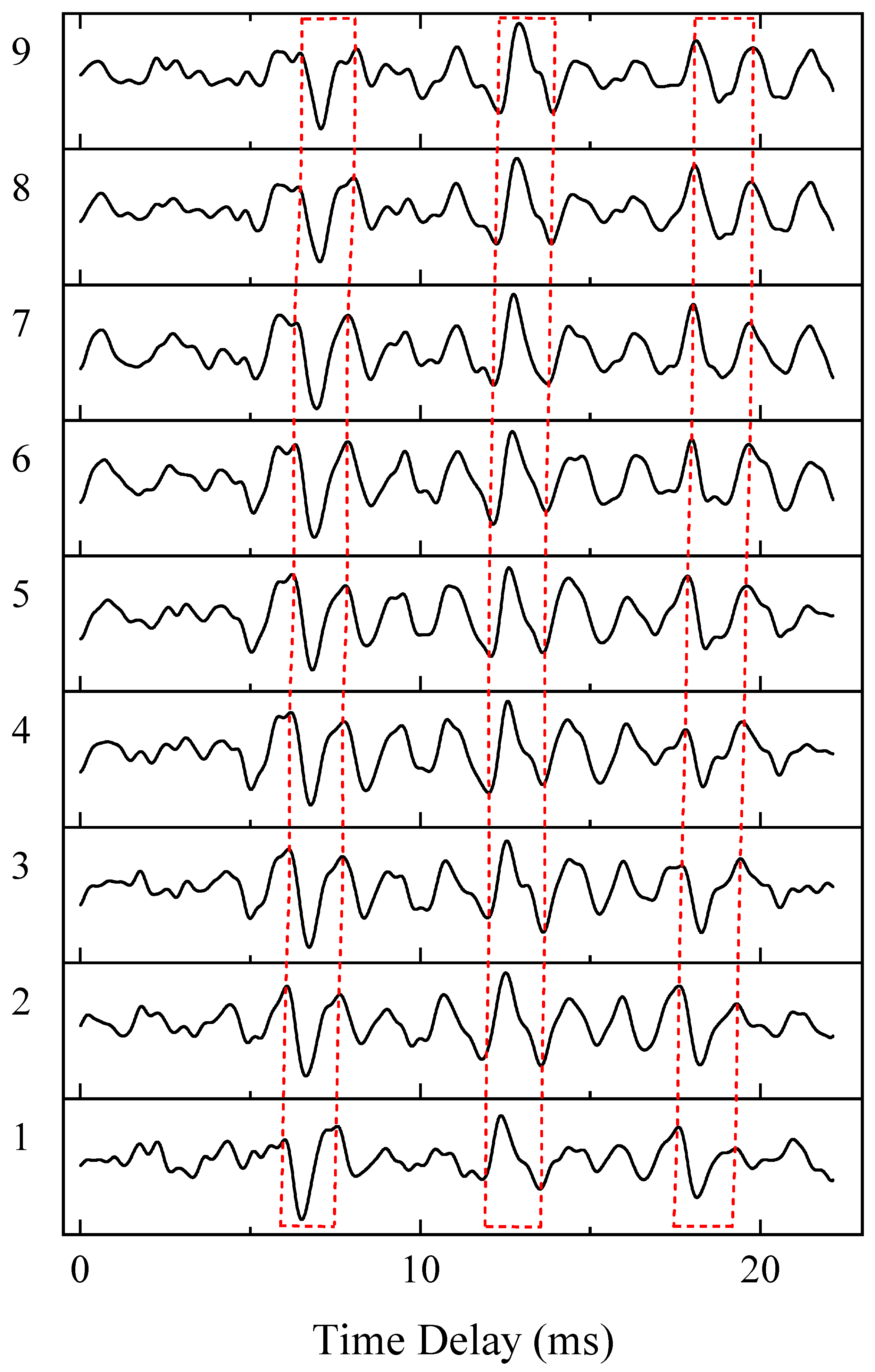
Figure 1. Multi-frame cross-correlation function. The pulses enclosed by the red dashed line in the middle are the cross-correlation pulses formed by the direct arrivals, and the left and right sides represent the cross-correlation pulses formed by the direct arrivals at one hydrophone and the multipath arrival at the other hydrophone.
Jmse 13 01764 g001
Figure 2. A weighted cubic spline is used to fit the observed time delay.
Jmse 13 01764 g002
Figure 3. Spatial distribution of hydrophones and the motion of the source.
Jmse 13 01764 g003
Figure 4. The correlogram of the simulation experiment.
Jmse 13 01764 g004
Figure 5. The iterative process of the proposed method. Different colorful lines correspond to different trajectories, where each color is used to distinguish one trajectory from another. (a) is the set of observations; (bd), respectively, represent the initial trajectories, the trajectories after the 6th iteration, and the final estimated trajectories.
Jmse 13 01764 g005
Figure 6. Convergence of the optimization under different initialization parameters. Each colorful line represents a different initialization setting. The tunable parameters include the maximum distance between observations in adjacent frames (proportional to the maximum source velocity), the maximum number of allowed gap frames (set to 5–10), and the minimum number of observations required in a trajectory (set to 3–6).
Jmse 13 01764 g006
Figure 7. Estimation results of four delay trajectories using different methods at PFP/PSNR of 76%/0.80. (a) The first trajectory; (b) The second trajectory; (c) The third trajectory; (d) The fourth trajectory.
Jmse 13 01764 g007
Figure 8. Estimation results of four delay trajectories using different methods at PFP/PSNR of 84%/0.75. (a) The first trajectory; (b) The second trajectory; (c) The third trajectory; (d) The fourth trajectory.
Jmse 13 01764 g008
Figure 9. Tracking performance analysis based on MC simulations. Each method plotted four curves corresponding to the probability of successfully estimating different numbers of trajectories.
Jmse 13 01764 g009
Figure 10. The correlogram formed by sea trial data.
Jmse 13 01764 g010
Figure 11. Multipath time-delay estimation results of sea trial data. (a) The superposition of correlogram and estimation results; (b) The estimation results of different methods.
Jmse 13 01764 g011
Table 1. Summary of notation.
SymbolDescription
x i t observations (correlation pulses)
I t the total number of observations in the tth frame
T n target trajectories
D n observations associated with trajectory T n
C n the total number of D n
s n , e n the start and end time of trajectory T n
observations considered as outliers
Disclaimer/Publisher’s Note: The statements, opinions and data contained in all publications are solely those of the individual author(s) and contributor(s) and not of MDPI and/or the editor(s). MDPI and/or the editor(s) disclaim responsibility for any injury to people or property resulting from any ideas, methods, instructions or products referred to in the content.