Full Waveform Inversion of Irregularly Sampled Passive Seismic Data Based on Robust Multi-Dimensional Deconvolution

Abstract

Full waveform inversion (FWI) comprehensively utilizes phase and amplitude information of seismic waves to obtain high-resolution subsurface medium parameter models, applicable to both active-source and passive-source seismic data. Passive-source seismic exploration, using natural earthquakes or ambient noise, reduces costs and environmental impact, with growing marine applications in recent years. Its rich low-frequency content makes passive-source FWI (PSFWI) a key research focus. However, PSFWI inversion quality relies heavily on accurate virtual source reconstruction. While multi-dimensional deconvolution (MDD) can handle uneven source distributions, it struggles with irregular receiver sampling. We propose a robust MDD method based on multi-domain stepwise interpolation to improve reconstruction under non-ideal source and sampling conditions. This approach, validated via an adaptive PSFWI strategy, exploits MDD’s insensitivity to source distribution and incorporates normalized correlation objective functions to reduce amplitude errors. Numerical tests on marine and complex scattering models demonstrate stable and accurate velocity inversion, even in challenging acquisition environments.

1. Introduction

Passive-source seismic exploration methodologies, characterized by low cost and environmentally benign operations, have been widely implemented in marine seismic exploration, engineering surveys, and environmental investigations. High-resolution velocity modeling of subsurface media using passive seismic data has attracted growing attention. High-quality reconstructed passive-source interferometric records serve as critical prerequisites for robust velocity inversion. Currently, seismic interferometry has emerged as a primary technique for passive seismic data processing, enabling the reconstruction of passive virtual source (PVS) records akin to active-source seismic records without requiring a priori knowledge of source locations or source–wavelet functions.

Claerbout first proposed treating any receiver as a virtual source to construct PVS records using recordings from other receivers [1]. Schuster subsequently systematized the theoretical framework of seismic interferometry, achieving PVS records synthesis and migration imaging, thereby expanding its applications [2]. Wapenaar et al. rigorously established the theoretical foundation of seismic interferometry through the unidirectional reciprocity theorem and Green’s function theory [3,4], systematically formalizing point-spread function theory and the workflow for MDD [5]. Numerical experiments demonstrated MDD’s efficacy in correcting non-uniform ambient noise distributions and enhancing Green’s function’s reconstruction accuracy for surface waves [6], solidifying MDD’s theoretical basis. Bakulin and Calvert innovated the virtual source method, eliminating reliance on source wavelet information in traditional approaches [7]. Vasconcelos et al. advanced deconvolutional interferometry theory, validating MDD’s superior performance in field data [8,9,10,11]. Ravasi et al. developed an MDD implementation without wavefield decomposition, improving algorithmic flexibility [12]. For ill-posed inverse problems, Luiken and Van Leeuwen incorporated Tikhonov regularization into a least-squares framework, suppressing overburden interferences and stabilizing Green’s functions [13]. There have recently been some MDD advancements. Vargas et al. pioneered time-domain MDD with physical constraints (reciprocity, causality) to reduce regularization parameter sensitivity, which successfully reconstructed PVS records using the noise data of subsalt structures [14].

Notably, both PVS record generation by cross-correlation interferometry and enhancement of reconstructed accuracy by MDD interferometry critically depend on high-quality, fully sampled passive seismic datasets. Consequently, high-precision seismic data interpolation constitutes a pivotal preprocessing step, with appropriately tailored interpolation methodologies being essential for achieving optimal results. Seismic data interpolation techniques are broadly categorized into prediction filter-based interpolation and compressed sensing-based interpolation. Compressed sensing-based interpolation effectively compresses the data, using sparse transformations to complete the interpolation. Herrmann and Hennenfent first introduced multi-scale, multi-directional curvelet transforms into seismic data interpolation [15]. Subsequently, Hennenfent’s team advanced non-uniform fast discrete curvelet transforms to directly process irregularly missing data [16]. Naghizadeh and Sacchi developed dip-guided filtering strategies based on multi-scale dip-consistency assumptions in the curvelet domain [17]. Yang and Zhang et al. integrated iterative hard/soft thresholding and projection onto convex sets (POCS) with curvelet transforms to establish noise-resilient, broadly applicable sparse optimization frameworks [18,19,20]. Recently, Wang et al. innovatively integrated Hankel matrix low-rank approximation with the Alternating Direction Method of Multipliers (ADMM), balancing data continuity and low-rank constraints to significantly improve noise robustness and computational efficiency [21].

Seismic interferometry and seismic data interpolation methodologies enable the acquisition of high-fidelity seismic datasets, which facilitate full waveform inversion (FWI) to resolve high-resolution subsurface velocity structures. FWI was initially conceptualized by Tarantola and gained prominence with advancements in high-performance computing [22]. Early research focused on active-source applications in time-domain and frequency-domain FWI, with frequency-domain implementations offering superior computational efficiency [23]. Bunks et al. pioneered multi-scale inversion through scale-optimized hierarchical workflows to enhance convergence [24]. Han obtained elastic wave full waveform inversion results from marine seismic data using wavefield separation [25]. Recently, passive-source seismic data inversion has emerged as a frontier in FWI research. Passive-source full waveform inversion (PSFWI) has been extensively applied to high-resolution structural imaging in natural seismogenic zones and tectonic fracture systems, for example, ambient noise adjoint tomography in the Los Angeles Basin [26], ambient noise surface-wave waveform imaging of the upper crust along the Weifang segment of the Tan-Lu Fault Zone [27], and high-resolution S-wave velocity, radial anisotropy, and Poisson’s ratio models derived from dense earthquake-station data at the eastern Tibetan Plateau margin [28]. Concurrently, deep learning techniques have been integrated into FWI frameworks through generative neural networks for velocity modeling, such as unsupervised learning to reduce initial model sensitivity, self-supervised architectures to mitigate local minima entrapment, and physics-constrained regularization to enhance inversion precision and generalization. These advancements progressively address challenges in low-frequency dependency, computational complexity, and solution non-uniqueness. Deep learning combined with FWI is gradually becoming a core tool for refined subsurface imaging [29,30,31,32,33,34,35]. Objective function innovations include time-domain convolutional and correlation-type formulations, broadening PSFWI adaptability [36,37]. For source parameter estimation, Sun et al. implemented diagonal preconditioning for source parameter recovery [38]. Others include elastic wave passive-source equivalent source inversion combined with source-independent elastic FWI [39] and iterative methods integrating geometric-mean reverse time migration with FWI [40]. Zhang et al. first hybridized seismic interferometry with FWI, demonstrating passive data’s capacity to supplement deep structural constraints for active-source model initialization [41], later analyzing parameter sensitivities for body-wave interferometric FWI [42]. Shang et al. achieved enhanced inversion results via improved multi-dimensional deconvolution integrating active–passive seismic datasets [43].

We propose a robust MDD and FWI framework based on dual-domain stepwise interpolation. The fundamental principles of the robust MDD interferometry integrated with stepwise interpolation are first introduced, followed by validation on a simple layered velocity model. A normalized correlation FWI objective function compatible with this methodology is subsequently formulated. Numerical tests are conducted on two benchmark models, the multi-layer Marmousi model and a complex metal ore deposit model characterized by intricate subsurface velocity heterogeneities. Experimental configurations simulate varying degrees of missing trace and heterogeneous source distributions, validating the method’s applicability and accuracy under non-ideal conditions. Our proposed method solves the low accuracy problem of PSFWI in the case of non-uniform distributions of passive sources and incomplete seismic data. We provide a solution for full waveform inversion of passive sources in complex acquisition situations and complex geologic conditions.

2. Methods

2.1. Robust Multi-Dimensional Deconvolution (RMDD) Seismic Interferometry Based on Multi-Domain Stepwise Interpolation

2.1.1. Traditional Seismic Interferometry

Processed raw seismic noise recordings can be reconstructed into PVS records resembling active-source records through seismic interferometry. In practical ambient noise data processing, cross-correlation seismic interferometry is commonly employed for wavefield reconstruction. Under the high-frequency approximation, the fundamental principle of cross-correlation seismic interferometry is expressed as follows [5]:

$$G(x_B,x_A,t)+G(x_B,x_A,-t)\approx {\displaystyle \frac{2}{\rho c}}{\displaystyle {\oint }_{\mathrm{Src}}G}(x_B,x_S,t)\ast G(x_A,x_S,-t)\mathrm{d}{x}_S,$$

(1)

where $G(x_B,x_A,t)$ denotes the Green’s function propagating from receiver A (acting as a virtual source) to receiver B, $-t$ denotes non-causal, ${\oint }_{\mathrm{Src}}$ denotes the source integration surface, and $G(x_B,x_S,t)$, $G(x_A,x_S,-t)$ correspond to the Green’s functions recorded at receiver B and receiver A, respectively, for a source $x_S$ located on ${\oint }_{\mathrm{Src}}$. $\ast$ denotes temporal convolution.

Equation (1) assumes a lossless medium and uniform source distribution, yielding significant errors and degraded reconstruction accuracy under non-uniform source configurations. In field seismic acquisitions, ambient noise sources typically exhibit non-uniform, non-random spatial distributions, resulting in poor reconstruction quality via cross-correlation interferometry. MDD seismic interferometry mitigates these artifacts caused by source distribution heterogeneity. The fundamental principle of MDD is expressed as follows [5]:

$$C_{v^s,\tilde{v}}(x_B,x_A,t)={\displaystyle {\int }_{S_{rec}}{G}^s}(x_B,x,t)\ast \mathsf{\Gamma }(x,x_A,t)\mathrm{d}x,$$

(2)

where

$$C_{v^s,\overline{v}}(x_B,x_A,t)={\displaystyle \sum _i{v}^s}\left(x_B,x_S^{(i)},t\right)\ast \overline{v}\left(x_A,x_S^{(i)},-t\right),$$

(3)

$$\mathsf{\Gamma }(x,x_A,t)={\displaystyle \sum _i\overline{p}}\left(x,x_S^{(i)},t\right)\ast \overline{v}\left(x_A,x_S^{(i)},-t\right),$$

(4)

where $C_{v^s,\overline{v}}(x_B,x_A,t)$ denotes the correlation function and $\mathsf{\Gamma }(x,x_A,t)$ denotes the point spread function (PSF), which are approximated in the MDD seismic interferometry of noise sources, $G^s(x_B,x,t)$ denotes the scattering Green’s function, and $S_{rec}$ is the absorption interface where the receivers are located. $x$ is one of the receivers, $x_S$ is the location of the source. $t$ is a time series. $\ast$ is the convolution symbol. $x_A$ and $x_B$ are two receivers deployed on the surface. $v^s\left(x_B,x_S^{(i)},t\right)$ denotes the scattering information from $x_S$ to $x_B$. $\overline{v}\left(x_A,x_S^{(i)},-t\right)$ denotes the direct information from $x_S$ to $x_A$. $\overline{p}\left(x,x_S^{(i)},t\right)$ denotes the pressures from $x_S$ to $x$.

Equations (2)–(4) demonstrate that MDD seismic interferometry shifts the integration surface from the passive-source domain to the receiver domain, thereby decoupling the influence of source distribution characteristics on reconstruction accuracy. This approach significantly reduces the dependence of PVS records’ fidelity on source-related parameters (e.g., source density, spatial coverage, and excitation energy), instead constraining reconstruction errors primarily to receiver array uniformity—a factor controllable through predefined surface acquisition geometries. By transferring the critical reconstruction constraint to anthropogenically manageable receiver layouts, the method alleviates the stringent prerequisites of passive-source seismic exploration and suppresses reconstruction artifacts caused by non-ideal source conditions.

2.1.2. RMDD Based on Multi-Domain Stepwise Interpolation

The analysis above reveals that MDD seismic interferometry exhibits strong dependence on receiver geometry, requiring densely and regularly distributed receivers. In practical passive-source seismic exploration, issues such as damaged receivers, trace gaps, and sparse receiver arrays necessitate seismic trace interpolation to regularize irregular geometries. However, interpolation solely in the common-shot domain fails to address all missing PVS records, as gaps in raw seismic traces prevent complete reconstruction of certain PVS, resulting in “blank shots” within the gather. A dual-domain transformation strategy is thus essential. After interpolating PVS records in the common-shot domain, the data are transformed to the common-receiver domain, converting blank-shot issues into trace-missing problems within common-receiver gathers. Secondary interpolation in this domain enables comprehensive data regularization across all PVS records.

In the approximate solution of noise-source MDD, the complete cross-correlated PVS records can be decomposed into two components: the PSF and the correlation function. Under missing trace conditions, PVS records reconstructed via cross-correlation interferometry exhibit both trace gaps and missing information at gap locations. To address this, we first extract the PSF (exhibiting linear kinematic characteristics) and correlation function (displaying curvilinear features) from the incomplete PVS records in the common-shot domain. A stepwise interpolation strategy is then applied. We use linear-feature interpolation to recover the PSF component, and use curvelet transform-based interpolation to reconstruct the correlation function. The interpolated results are subsequently transformed to the common-receiver domain, where the blank-shot issue manifests as receiver-domain trace gaps. The stepwise interpolation process is repeated in this domain to finalize the regularization of all PVS records. This dual-domain, feature-specific interpolation approach ensures comprehensive reconstruction of missing PVS records while preserving the kinematic and dynamic attributes of both PSF and correlation components.

The matrix formulation of ambient noise MDD can be approximated as

$$C=G^s\mathsf{\Gamma },$$

(5)

where $G^s$ denotes the scattering Green’s function. The principle of the stepwise interpolation method based on the characterization of the PSF and the correlation function is as follows:

$${\mathsf{\Gamma }}_{full}=L{\mathsf{\Gamma }}_{MDD}^{obs},$$

(6)

$$\begin{gathered} C_{full}^k=C_{MDD}^{obs}+[I-M(t,x)]C^T{T}_{k}C{C}_{full}^{k-1}, \\ \mathrm{k}=1,2,\dots ,\mathrm{N}, \end{gathered}$$

(7)

where ${\mathsf{\Gamma }}_{full}$ denotes the complete PSF component after linear feature interpolation and ${\mathsf{\Gamma }}_{MDD}^{obs}$ denotes initial PSF reconstructed from missing seismic data. $C_{full}^k$ denotes the complete correlation function component after the k-th interpolation iteration. $C_{MDD}^{obs}$ denotes the initial correlation function reconstructed from missing seismic data. $C_{full}^{k-1}$ denotes the complete correlation function component after the (k − 1)-th interpolation iteration. When k = 1, $C_{full}^{k-1}$ equals $C_{MDD}^{obs}$. $L$ denotes linear feature interpolation, I denotes the identity matrix, $M(t,x)$ denotes non-missing seismic trace positions, $C$ and $C^T$ denote curvelet transform and inverse curvelet transform, k is the number of iterations, and $T_k$ is denoted by (8):

$$T_k=\left\{\begin{array}{ll}(S_k-\lambda \mid S_k{\mid }_{max})S_k,\hfill & \mid S_k\mid >\lambda \mid S_k{\mid }_{max}\hfill \\ 0,\hfill & \mid S_k\mid \le \lambda \mid S_k{\mid }_{max}\hfill \end{array}\right.,$$

(8)

where $S_k$ denotes curvelet coefficients, $\mid S_k{\mid }_{max}$ denotes the maximum curvelet coefficients, and $\lambda$ denotes the threshold coefficient (ranging between 0 and 1).

Substituting Equations (6) and (7) into Equation (5) yields the RMDD of stepwise interpolation.

$$C_{full}^k=G^s{\mathsf{\Gamma }}_{full}.$$

(9)

A comparative interpolation analysis employing the curvelet interpolation method and stepwise interpolation approach is conducted on a layered velocity model (Figure 1a). The model dimensions are 800 m × 1910 m with a grid spacing of 10 m. A total of 192 receivers are deployed at 10 m intervals. Under idealized noise-source distribution conditions (Figure 1b), 300 ambient noise sources are randomly distributed within the subsurface zone spanning a depth of 400–800 m and lateral extent of 0–1910 m. Key acquisition parameters include source wavelet frequency band: 0–30 Hz, sampling interval: 0.001 s, recording duration: 300 s, and data incompleteness: 50% random traces missing.

Figure 2 compares cross-correlation reconstructions and MDD results obtained via different interpolation methods. The analysis reveals superior accuracy of the stepwise interpolation in recovering the PSF component. This precision in PSF interpolation significantly enhances MDD fidelity. MDD with stepwise interpolation achieves markedly higher accuracy than curvelet-only interpolation, closely approximating MDD results derived from fully sampled seismic traces. The stepwise-interpolated MDD outputs exhibit enhanced waveform clarity.

2.2. PSFWI Based on RMDD

FWI enables precise characterization of subsurface velocity structures by leveraging travel-time, phase, and amplitude information from seismic wavefields, outperforming travel-time tomography in resolution and accuracy due to its comprehensive utilization of waveform kinematics and dynamics. Traditional FWI formulations typically employ L2-norm-based objective functions [24]:

$$E\left(m\right)={\displaystyle \frac{1}{2}}\Vert u\left(m\right)-d{\Vert }^2,$$

(10)

where $u\left(m\right)$ and $d$ denote observed data and synthetic data, and $m$ denotes the velocity parameters of the subsurface medium. The gradient is expressed as

$${\displaystyle \frac{\partial E}{\partial m}}=〈{\displaystyle \frac{\partial u}{\partial m}},u-d〉.$$

(11)

where $〈{\displaystyle \frac{\partial u}{\partial m}},u-d〉$ represents the inner product of ${\displaystyle \frac{\partial u}{\partial m}}$ and $u-d$. Conventional FWI based on traditional objective functions requires precise source wavelet estimation, as inversion results are highly sensitive to source wavelet errors, which may cause model updates to deviate from true subsurface structures or even lead to convergence failure and local minima entrapment. In passive-source seismic data, source wavelets are inherently difficult to characterize. Even when employing cross-correlation seismic interferometry to reconstruct PVS gathers, accurate estimation of the embedded source wavelets remains challenging. PSFWI utilizes naturally occurring seismic energy (e.g., microseisms, ambient noise, or teleseismic events) to invert subsurface parameters. Its advantages include cost-effectiveness and environmental sustainability due to reliance on natural sources, low-frequency-rich illumination enhancing deep structural resolution and compensating for active-source low-frequency deficiencies, and multi-azimuth illumination from stochastic source distributions, improving imaging of complex geometries. However, a low signal-to-noise ratio (SNR) necessitates large datasets for stable inversion. Source parameter uncertainties (e.g., location, timing, wavelet) amplify inversion nonlinearity. Non-uniform source distributions introduce reconstruction artifacts in interferometric methods. To mitigate source wavelet dependency, source-independent objective functions have been proposed for PVS records from cross-correlation seismic interferometry. However, in practical scenarios characterized by non-uniform source distributions, MDD achieves superior accuracy by generating wavelet-free interferometric records. This methodology, when integrated with normalized correlation objective functions, capitalizes on its insensitivity to source signatures and amplitude fidelity to yield enhanced inversion precision.

2.2.1. Source-Independent Time-Domain PSFWI

In conventional cross-correlation interferometry, the reconstructed PVS records inherently suffer from unknown source wavelet signatures, rendering conventional FWI inapplicable. Consequently, source-independent FWI methods are typically employed. Source-independent FWI utilizes a convolution-type objective function based on the least-squares framework. This approach mitigates the impact of wavelet inaccuracies by convolving the source wavelets of synthetic data and observed data within the objective function [36].

$$E={\displaystyle \frac{1}{2}}{\displaystyle \sum _i^{ns}{\displaystyle \sum _j^{nr}\parallel }}{u}_{i,j}\ast d_{i,k}-d_{i,j}\ast u_{i,k}{\parallel }^2,$$

(12)

is equivalent to

$$E={\displaystyle \frac{1}{2}}{\displaystyle \sum _i^{ns}{\displaystyle \sum _j^{nr}\parallel }}{G}_{i,j}^u\ast s_{i,j}^u\ast G_{i,k}^d\ast s_{i,k}^d-G_{i,j}^d\ast s_{i,j}^d\ast G_{i,k}^u\ast s_{i,k}^u{\parallel }^2,$$

(13)

where $u=G^u\ast s^u,$ $d=G^d\ast s^d,$ denote observed data and synthetic data. $G$ denotes Green’s function. $s$ denotes the source wavelet. i denotes the location of PVS. j and k denote the location of receivers. $ns$ and $nr$ denote the number of PVS and receivers. The gradient expression with respect to the velocity parameters is given as follows:

$${\displaystyle \frac{\partial E}{\partial v}}={\displaystyle \sum _i^{ns}{\displaystyle \sum _j^{nr}\left[\left(\frac{\partial u_{i,j}}{\partial v}\ast d_{i,k}\right)\cdot r_{i,j}-\left(d_{i,j}\ast \frac{\partial u_{i,k}}{\partial v}\right)\cdot r_{i,j}\right]}},$$

(14)

where

$$r_{i,j}=u_{i,j}\ast d_{i,k}-d_{i,j}\ast u_{i,k}.$$

(15)

The adjoint source expressions can be formulated as the following two equations:

$${r_{i,j}}^{\prime }=d_{i,k}\otimes (u_{i,j}\ast d_{i,k}-d_{i,j}\ast u_{i,k}),$$

(16)

$${r_{i,j}}^{″}=-d_{i,j}\otimes (u_{i,j}\ast d_{i,k}-d_{i,j}\ast u_{i,k}).$$

(17)

where $\otimes$ is a relational operator. However, while such methodologies partially mitigate source wavelet effects, they fail to fully eliminate distortions caused by source wavelet perturbations during the inversion process. These constrain the resolution and reliability of the inverted results.

2.2.2. Normalized Correlation PSFWI Based on RMDD (RMDD-NCPSFWI)

In practical PSFWI, conventional approaches face two critical challenges. First, while cross-correlation-based PVS records imposes minimal constraints on receiver geometry, its accuracy is inherently limited by non-uniform noise-source distributions, leading to unreliable inversion results. Second, MDD significantly improves PVS records’ fidelity but requires uniform receiver arrays—a condition rarely met in field surveys due to irregular geophone layouts. To address these dual limitations, a RMDD method based on dual-domain stepwise interpolation is proposed. Additionally, a normalized correlation PSFWI approach grounded in RMDD is introduced to mitigate amplitude-related distortions. We chose NCPSFWI rather than source-independent time-domain PSFWI because NCPSFWI can mitigate the effects of amplitude inaccuracies, whereas source-independent time-domain PSFWI is susceptible to the influence of the reference channel and is less sensitive to the wavelet. The wavelet obtained from the RMDD method is known. This is an advantage of the RMDD method.

This methodology achieves high-fidelity reconstruction of scattered Green’s functions, enabling flexible convolution with known-frequency wavelets during subsequent inversion. The framework significantly enhances adaptability to source characteristics in PSFWI. Furthermore, to address the pervasive challenge of amplitude misalignment, the normalized correlation PSFWI method is introduced to effectively mitigate amplitude distortions. By integrating amplitude regularization into the objective function, the inversion accuracy and stability are significantly enhanced. The objective function formulation is expressed as follows [37]:

$$E=-{\displaystyle \frac{1}{2}}{\displaystyle \sum _i^{ns}{\displaystyle \sum }_j^{nr}}[-{\widehat{u}}_{i,j}\cdot {\widehat{d}}_{i,j}],$$

(18)

where ${\widehat{u}}_{i,j}$ and ${\widehat{d}}_{i,j}$ denote the normalized simulated data and the reconstructed PVS records. ${\widehat{u}}_{i,j}^2={\displaystyle \frac{u_{i,j}^2}{\parallel u_{i,j}^2\parallel }}$ and ${\widehat{d}}_{i,j}^2={\displaystyle \frac{d_{i,j}^2}{\parallel d_{i,j}^2\parallel }}$. i and j denote the location of PVS and the location of receivers. $ns$ and $nr$ denote the number of PVS and receivers.

Combining (9), (18) can be written as

$$E=-{\displaystyle \frac{1}{2}}{\displaystyle \sum _i^{ns}{\displaystyle \sum }_j^{nr}}[-{({\widehat{G}}_{i,j}^s)}^u\ast {\widehat{s}}_{i,j}^u\cdot {({\widehat{G}}_{i,j}^s)}^d\ast {\widehat{s}}_{i,j}^d],$$

(19)

where ${({\widehat{G}}_{i,j}^s)}^u$ and ${({\widehat{G}}_{i,j}^s)}^d$ denote the scattering Green’s function of the normalized simulated data and the scattering Green’s function of the observed data, obtained by multi-dimensional deconvolution after two-domain stepwise interpolation. ${\widehat{s}}_{i,j}^u$ and ${\widehat{s}}_{i,j}^d$ denote the amplitude-normalized source wavelet functions of the synthetic data and observed data, respectively. The normalization here is applied to the entire convolution of Green’s function and the source wavelet function.

The gradient of expression (18) with respect to the velocity parameters is given as follows:

$${\displaystyle \frac{\partial E}{\partial v}}={\displaystyle \sum _i^{ns}{\displaystyle \sum _j^{nr}\left[\frac{\partial {\widehat{u}}_{i,j}}{\partial v}\cdot {\overline{r}}_{i,j}\right]}},$$

(20)

where ${\overline{r}}_{i,j}$ is the adjoint source:

$${\overline{r}}_{i,j}={\displaystyle \frac{1}{‖u_{i,j}‖}}\left[{\widehat{u}}_{i,j}\left({\widehat{u}}_{i,j}\cdot {\widehat{d}}_{i,j}\right)-{\widehat{d}}_{i,j}\right]$$

(21)

The MDD seismic interferometry method based on stepwise interpolation enables the recovery of more accurate scattered Green’s functions. In subsequent PSFWI, these Green’s functions can be convolved with a known wavelet to enhance inversion accuracy. By integrating a normalized correlation full waveform objective function, the method mitigates the impact of amplitude inaccuracies in observed records, thereby yielding higher-precision PSFWI results.

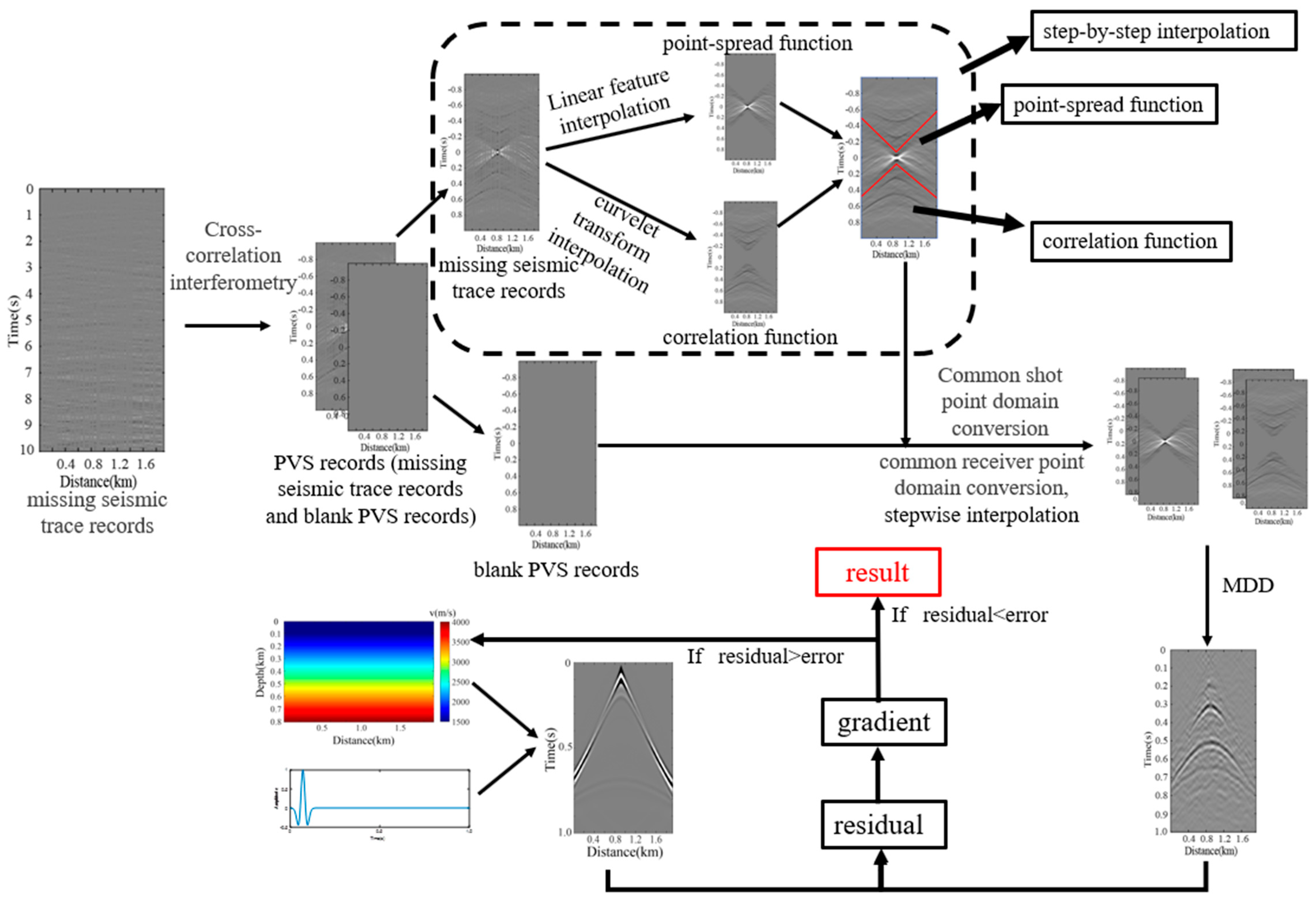
The entire technical approach is illustrated in Figure 3.

3. Results

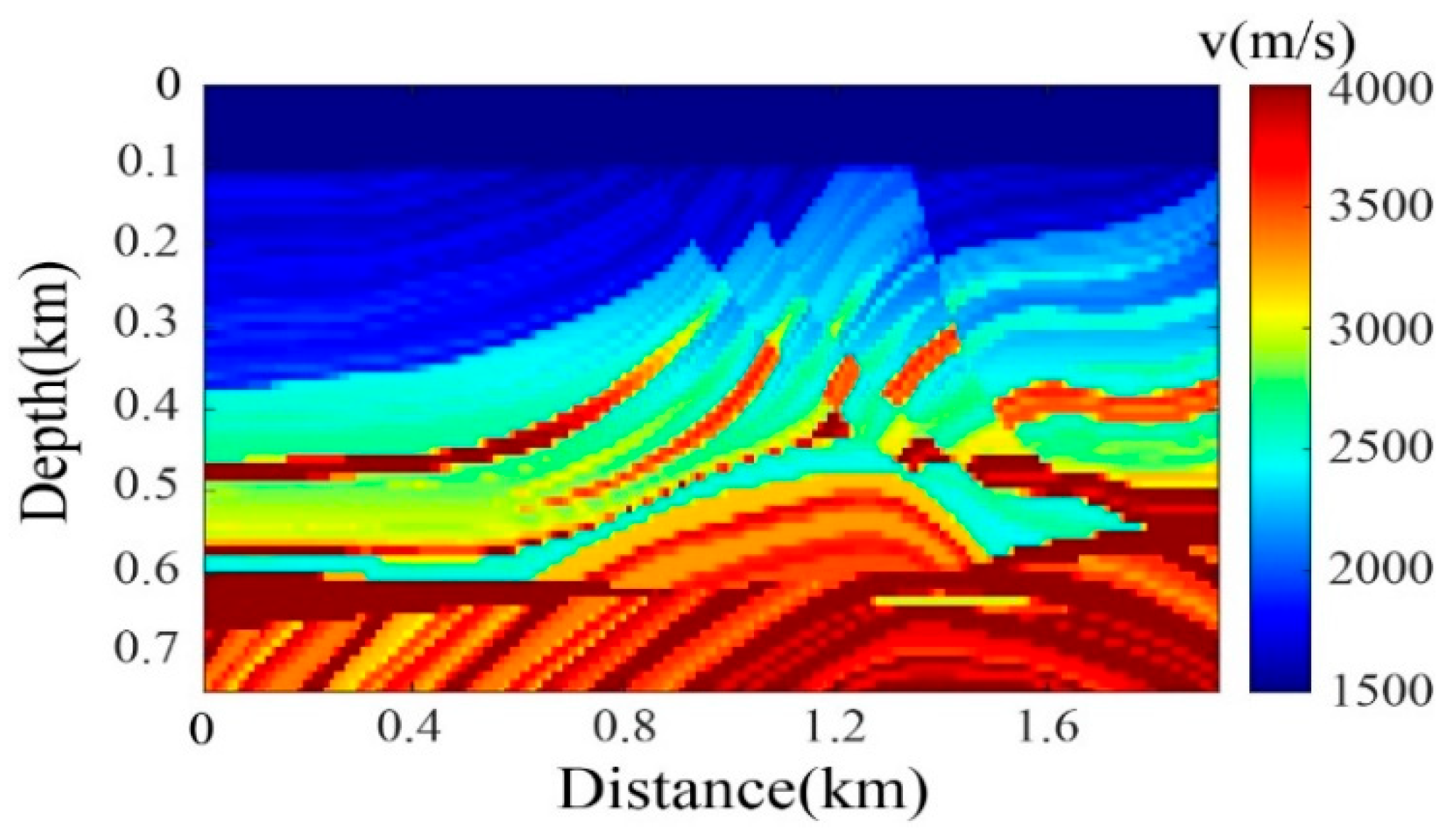
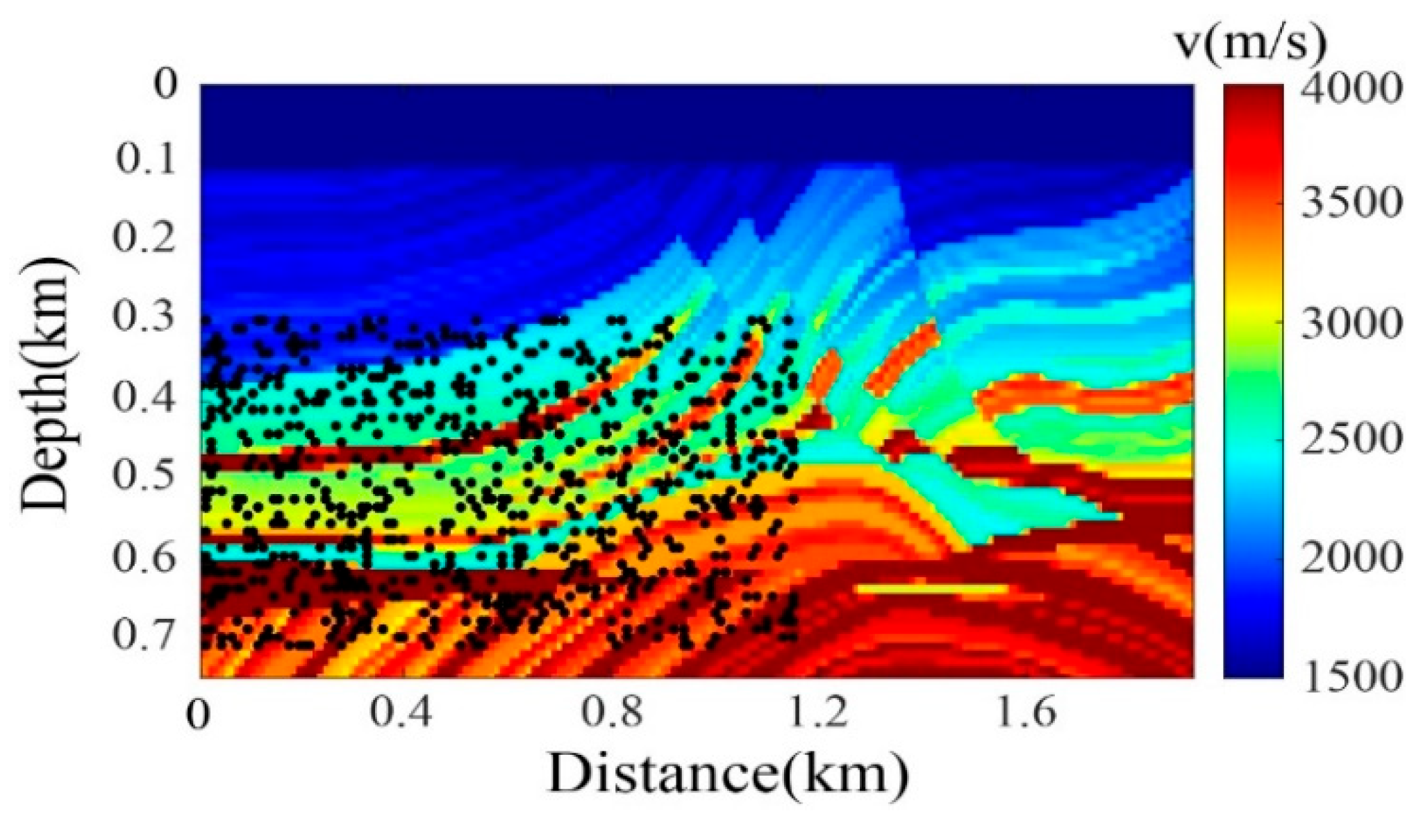
Experiments were conducted on the marine Marmousi model (Figure 4), with model dimensions of 830 m × 1910 m (including a 100 m water layer) and a grid spacing of 10 m. Receivers were deployed at 10 m intervals, totaling 192 receivers. To address receiver sparsity challenges in wavefield reconstruction, common-shot domain to common-receiver domain transformations were implemented, and curvelet-transform interpolation and stepwise interpolation methodologies were employed to regularize irregularly sampled data.

3.1. Idealized Passive-Source Distribution Testing

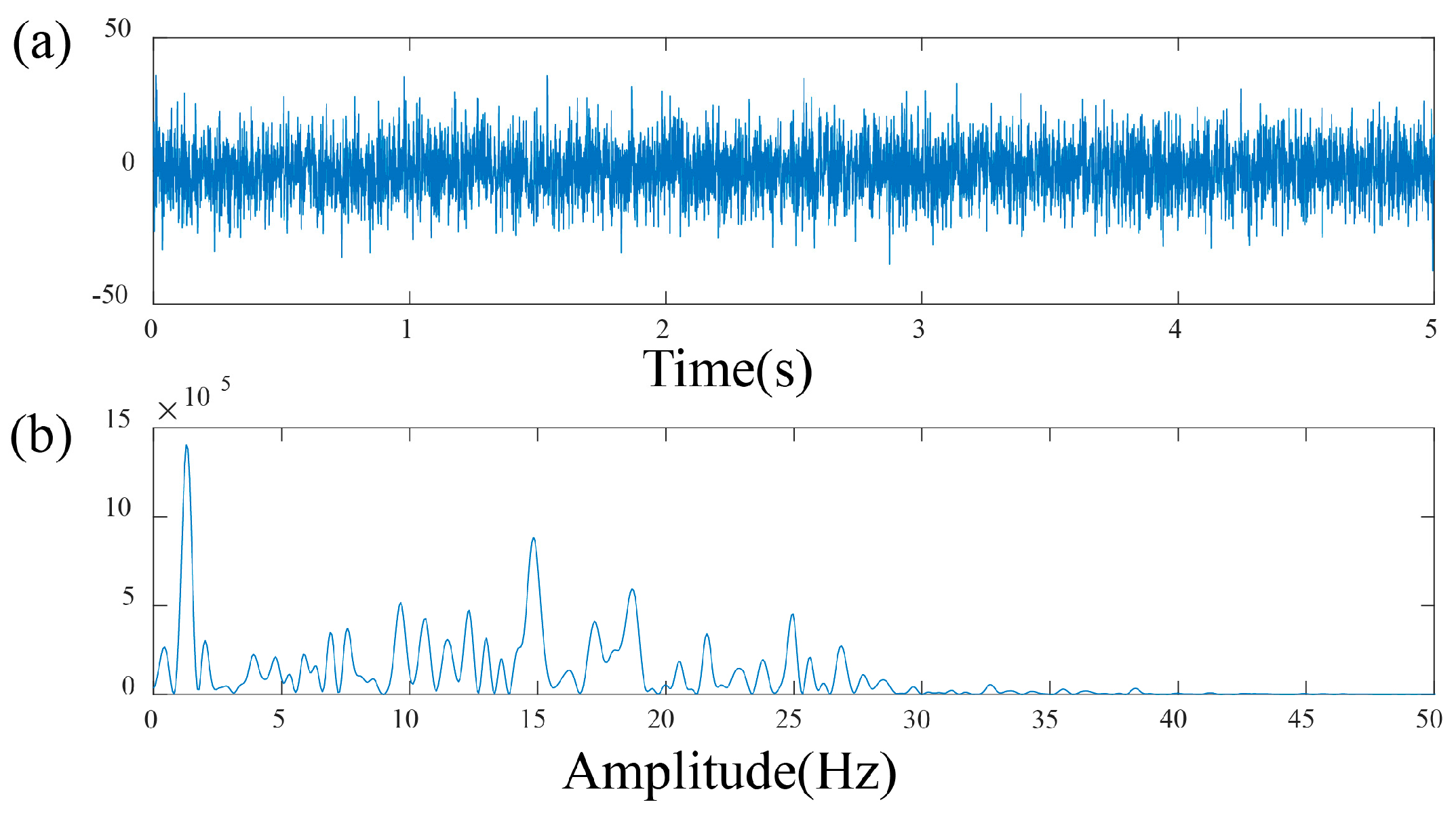
Under conditions of idealized random noise-source distribution, sources were randomly positioned within the subsurface zone spanning a depth of 300–700 m and lateral extent of 0–1910 m (Figure 5). The configuration included 800 ambient noise sources, source wavelet frequency band: 0–30 Hz, sampling interval: 0.001 s, and acquisition duration: 900 s. Two data incompleteness scenarios were simulated: 20% random traces missing and 50% random traces missing. The noise-source wavelet and its spectrum are shown in Figure 6. In the time domain, it manifests as an irregular noise signal. In the frequency domain, its frequency distribution is also non-concentrated within the 0–30 Hz range.

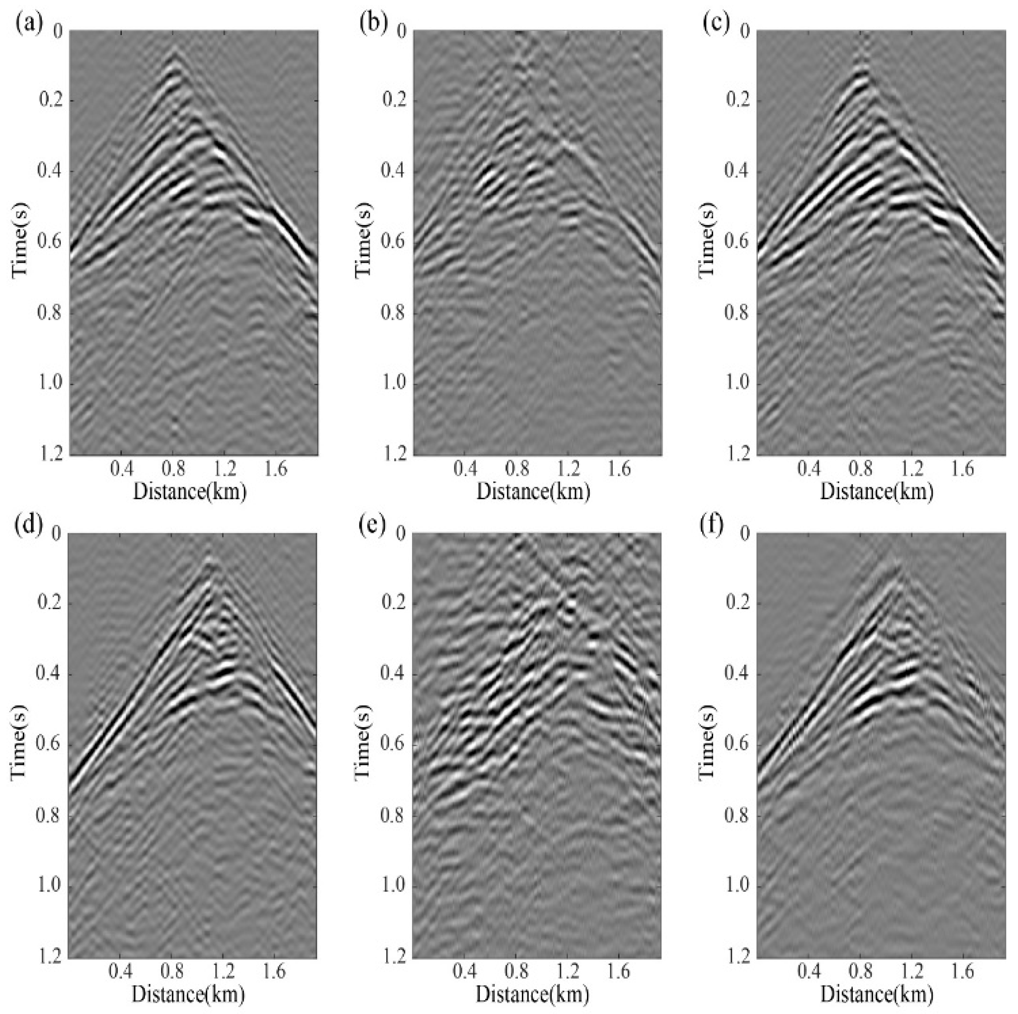
Under the condition of ideal random distribution of passive seismic sources, Marmousi modeling was conducted to generate synthetic seismic data. Subsequently, 20% and 50% of trace records were randomly removed to simulate missing data scenarios. The cross-correlation interferometry method was employed to reconstruct PVS records from the incomplete data. Two distinct interpolation approaches were implemented: (1) dual-domain transformation combined with curvelet-transform interpolation applied to the entire PVS records, and (2) dual-domain transformation combined with a stepwise interpolation methodology that separately processes PSF exhibiting linear characteristics and the correlation function demonstrating curved features. The reconstructed records were then subjected to MDD seismic interferometry. Comparative tests focusing on the originally missing trace positions (where blank shots in the original dataset provided intuitive contrast) were performed for both 20% and 50% missing trace scenarios (as illustrated in Figure 7).

Through comparative analysis of Figure 7a–c, it is evident that under low missing trace ratio scenarios (20%), conventional curvelet interpolation can partially reconstruct valid signal components, while the stepwise interpolation method achieves reconstruction accuracy comparable to MDD results from complete datasets. The comparison of Figure 7d–f demonstrates that in high missing trace ratio conditions (50%), pure curvelet interpolation fails to effectively recover coherent wavefield features, whereas the stepwise interpolation maintains high-fidelity reconstruction performance, exhibiting remarkable consistency with MDD benchmarks derived from intact data. Systematic evaluation reveals that the stepwise interpolation methodology exhibits strong robustness under severe data-loss scenarios, sustaining exceptional reconstruction precision in MDD records even with extreme trace depletion. This differential performance highlights the method’s adaptive capability.

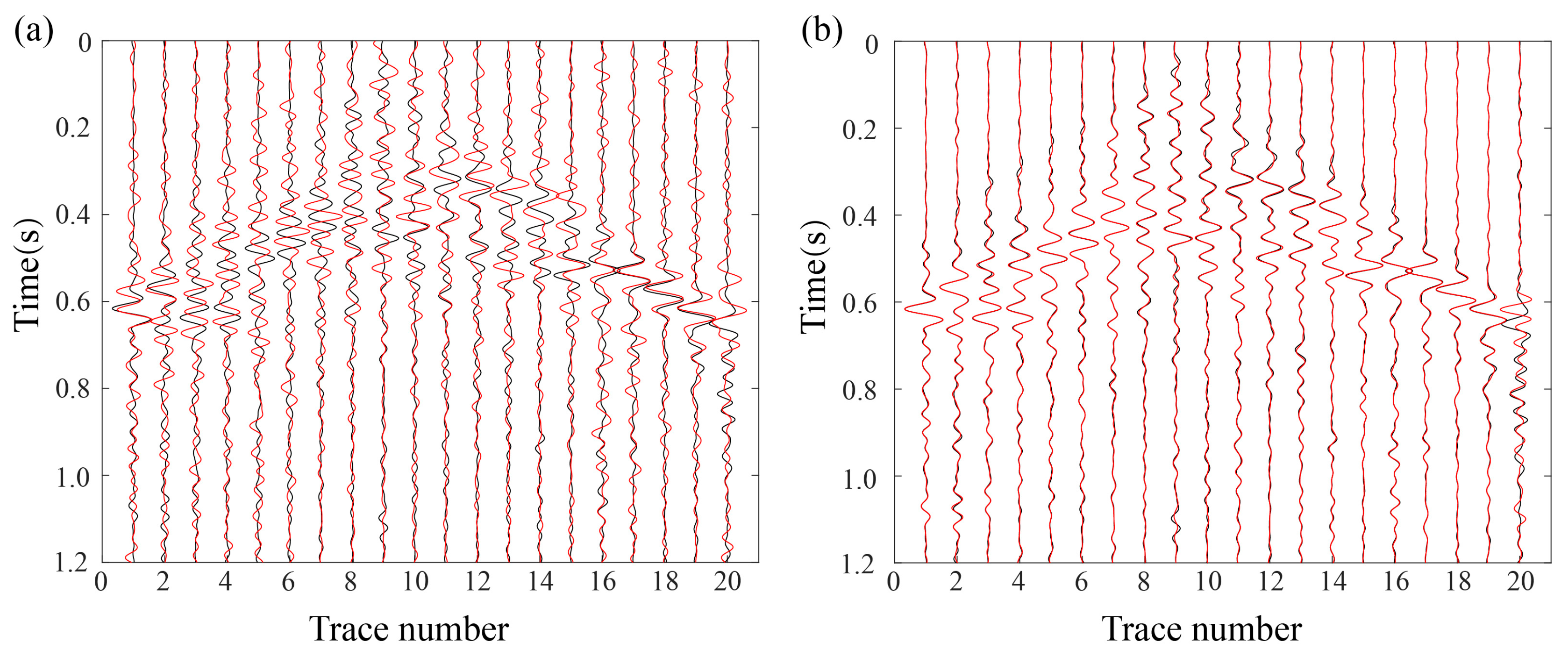
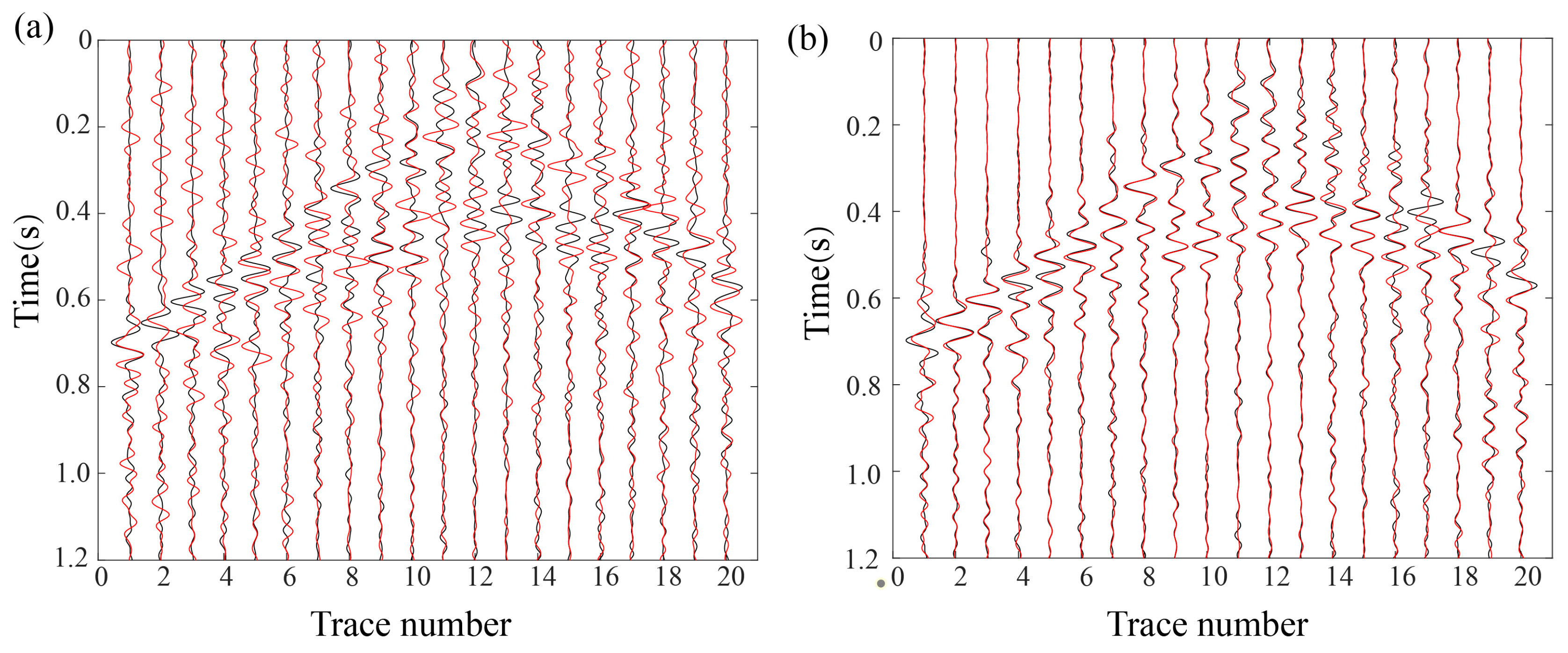
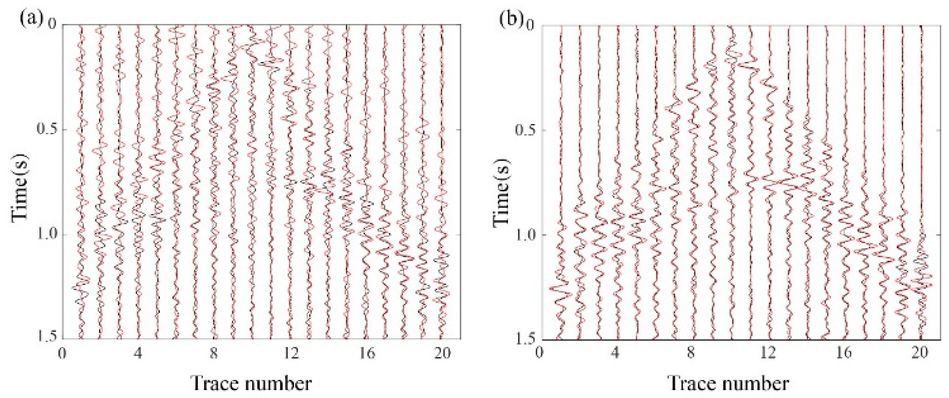
To more prominently demonstrate the superiority of the RMDD method, a comparative display of the trace waveforms pertaining to Figure 7 is provided in Figure 8 and Figure 9.

Figure 10 defines the initial velocity model for subsequent inversion analysis. MDD reconstructed records obtained through curvelet-transform interpolation and stepwise interpolation were sequentially convolved with 5 Hz, 10 Hz, and 15 Hz Ricker wavelets to implement multi-scale PSFWI (Figure 11). Comparative evaluation of inversion results was conducted for different missing trace ratios (20% vs. 50%) and interpolation methodologies. The active-source records of 50% missing trace inversion results were further benchmarked against active-source reference records through waveform similarity analysis (Figure 12).

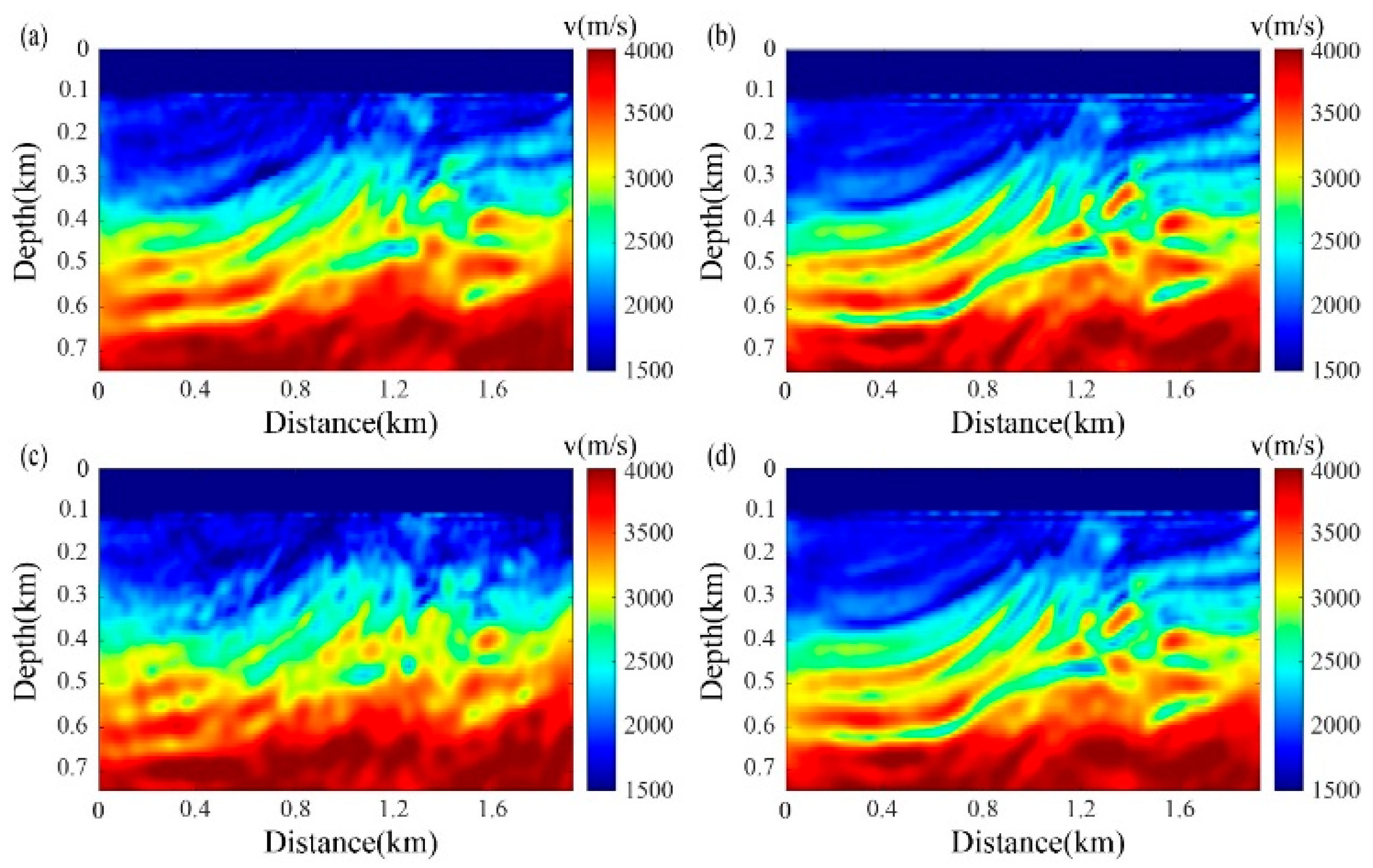
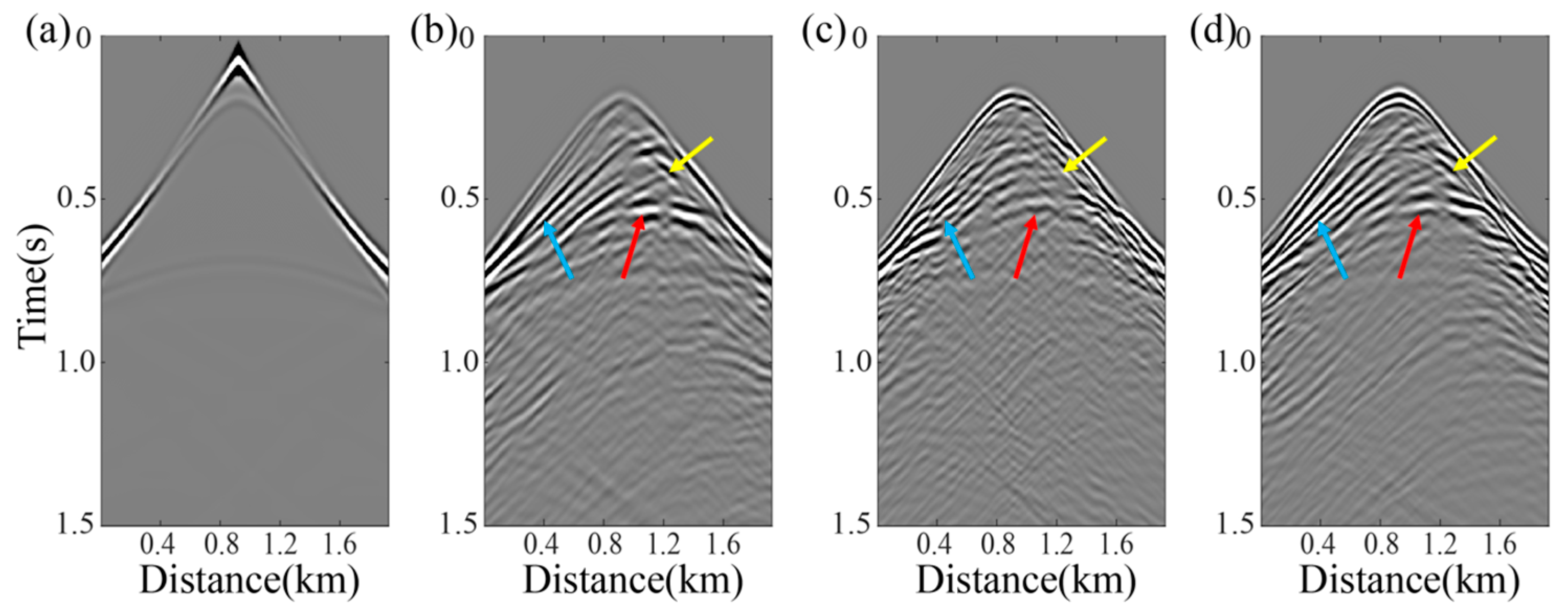
Through comparative analysis of Figure 11a–d, it can be observed that the curvelet-transform interpolation method yields satisfactory inversion results when dealing with limited missing trace scenarios. Under ideal source distribution conditions, it demonstrates reasonable capability in reconstructing macro-scale velocity structures, yet shows insufficient resolution in delineating fine-scale stratigraphic features of velocity layers. However, in cases of severely missing traces, the method struggles to delineate coherent velocity layer information and fails to construct effective large-scale velocity models. In contrast, the RMDD of the stepwise interpolation approach exhibits robust performance, maintaining high-quality PSFWI results across varying degrees of randomly missing traces. This method demonstrates superior resolution in both velocity layer boundary characterization and fault structure imaging. As indicated by the arrows in Figure 12, the progressive interpolation achieves notably higher precision compared to the curvelet-based method, along with enhanced adaptability to complex acquisition scenarios. Figure 12 verifies the applicability of the NCPSFWI objective function.

3.2. Non-Idealized Passive-Source Distribution Testing

Non-uniform source distribution leads to degraded reconstruction accuracy of seismic records, as incomplete effective information increases interpolation complexity. Therefore, under non-ideal noise-source distribution conditions, it becomes imperative to validate the applicability of the proposed methodology. Noise sources were randomly positioned within the subsurface zone spanning a depth of 300–700 m and lateral extent of 0–1150 m (Figure 13). Passive sources cover only 60% of the lateral spatial range. The configuration included 800 ambient noise sources, source wavelet frequency band: 0–30 Hz, sampling interval: 0.001 s, and acquisition duration: 900 s. Two data incompleteness scenarios were simulated: 20% random traces missing and 50% random traces missing.

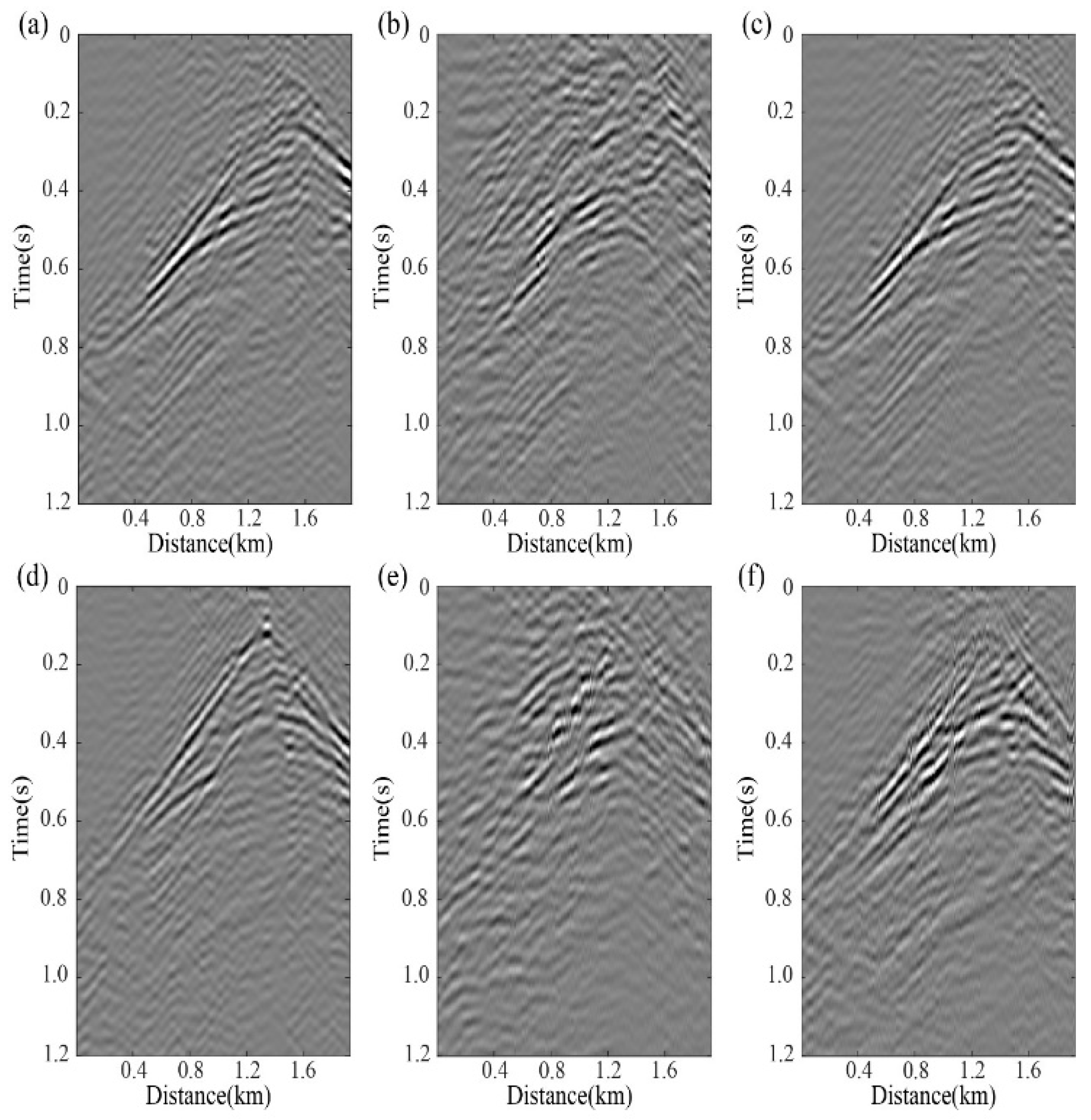
Under the condition of non-ideal random distribution of passive seismic sources, Marmousi modeling was conducted to generate synthetic seismic data. Subsequently, 20% and 50% of trace records were randomly removed to simulate missing data scenarios. The cross-correlation interferometry method was employed to reconstruct PVS records from the incomplete data. Two distinct interpolation approaches were implemented: (1) dual-domain transformation combined with curvelet-transform interpolation applied to the entire PVS records, and (2) dual-domain transformation combined with the stepwise interpolation methodology. The reconstructed records were then subjected to MDD seismic interferometry. Comparative tests focusing on the originally missing trace positions (where blank shots in the original dataset provided intuitive contrast) were performed for both 20% and 50% missing trace scenarios (as illustrated in Figure 14). The non-ideal distribution of noise sources leads to more complexity in reconstructing the records.

Comparative analysis of Figure 14a,b,d and Figure 14e reveals significant limitations in the pure curvelet-transform-based interpolation method under low missing trace conditions (20%). The reconstruction accuracy markedly deteriorates, failing to adequately recover phase and amplitude characteristics of seismic signals. When missing traces increase to 50%, the SNR of reconstructed records plummets, with effective reflections being obscured by noise and rendered nearly unrecognizable. However, as demonstrated by Figure 14a,c,d,f, the RMDD strategy maintains high-fidelity seismic signal recovery even under high trace-depletion scenarios (50%). The interpolated records exhibit strong consistency with MDD results from complete datasets in three key aspects—waveform coherence, event continuity of seismic phases, and energy distribution patterns. This validates the robust adaptability of RMDD method to non-uniform source distributions.

To more prominently demonstrate the superiority of the RMDD method, a comparative display of the trace waveforms pertaining to Figure 14 is provided in Figure 15 and Figure 16.

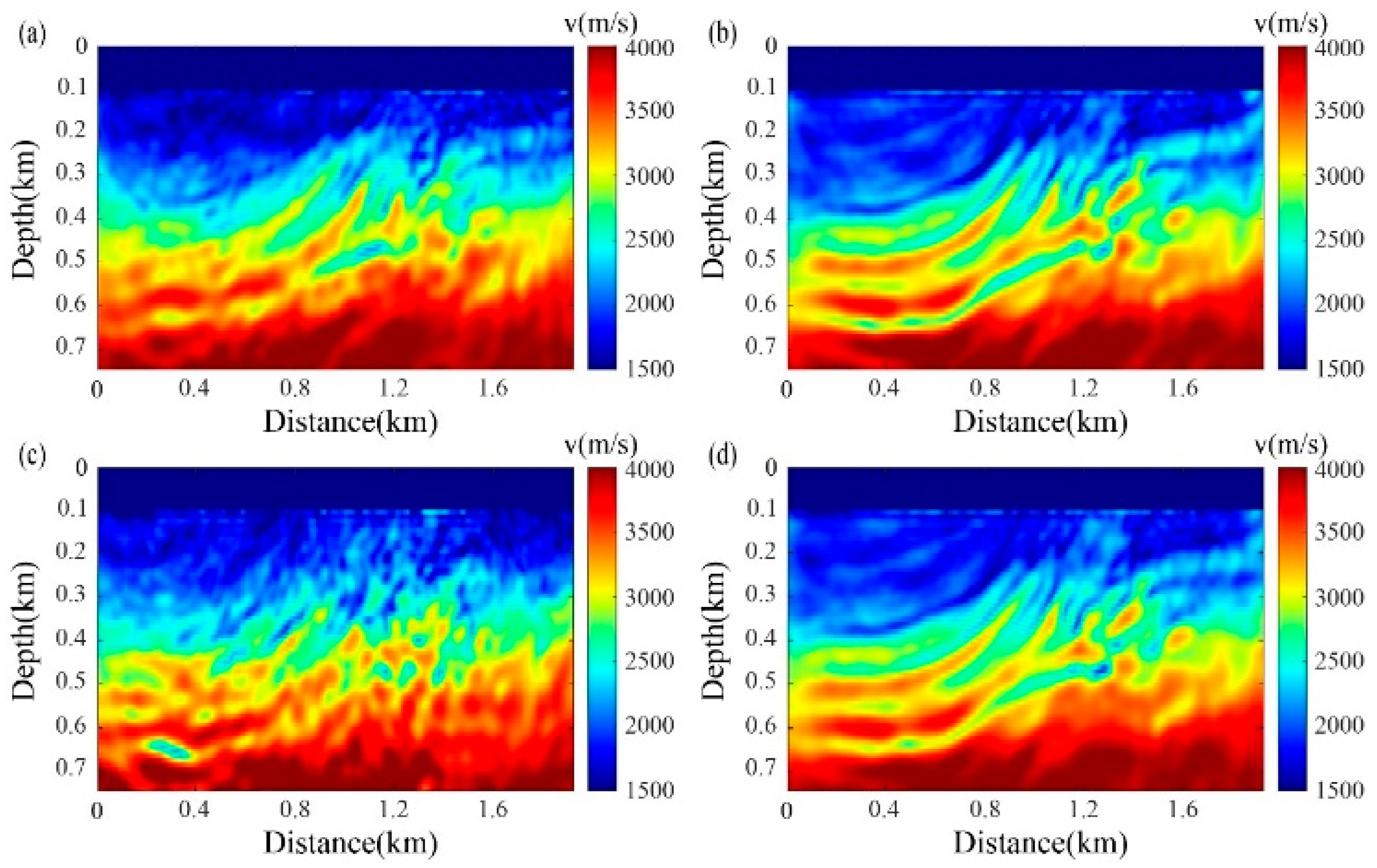
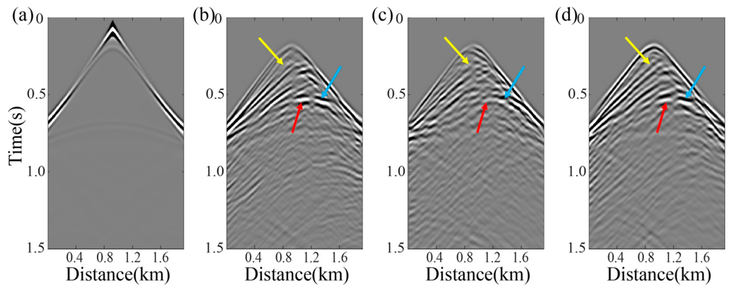
Figure 10 defines the initial velocity model for subsequent inversion analysis. MDD-reconstructed records—derived from both curvelet-transform interpolation and stepwise interpolation under non-ideal source distribution conditions—were sequentially convolved with 5 Hz, 10 Hz, and 15 Hz source wavelets to execute multi-scale PSFWI (Figure 17). Inversion results obtained using different interpolation methods were systematically compared across trace-depletion scenarios (20% and 50% missing traces). Furthermore, inversion outcomes with 50% missing traces were benchmarked against active-source reference records (Figure 18).

Comparative analysis of Figure 17a–d demonstrates that under non-ideal noise-source distribution conditions, the curvelet-interpolation method fails to produce viable inversion results regardless of trace depletion severity (20% or 50%). While partial recovery of stratigraphic horizons and fault structures is achievable with 20% missing traces, the method essentially loses interpretative value when trace depletion increases to 50%. In contrast, RMDD methodology exhibits remarkable stability, consistently delivering high-quality PSFWI results across all trace-missing scenarios. This approach effectively resolves both deep stratigraphic boundaries and shallow structural features. Further validation through the arrow-annotated regions in Figure 18 reveals that under non-ideal source distribution, RMDD maintains precise velocity model reconstruction capabilities, whereas curvelet-based interpolation yields nearly unusable results.

3.3. Complex Strong-Scattering Model

In the complex strong-scattering model, the subsurface structures exhibit intricate complexity characterized by abundant diffracted waves and scattered wavefields, while the reflected wave energy remains relatively weak. The effective low-frequency components are particularly susceptible to noise contamination. When conducting numerical simulations on such strong-scattering models, these compounded factors result in heightened complexity in passive-source seismic data reconstruction, manifesting as ambiguous discernibility of valid seismic signals within the recorded datasets.

To further evaluate the applicability and accuracy of the proposed method under complex geological conditions, PSFWI tests based on multi-domain stepwise interpolation were conducted on a complex strong-scattering model (Figure 19). The model spans 2520 m × 7520 m with a grid size of 20 m. Receivers were deployed at 20 m intervals, totaling 376 stations. Under the assumption of ideally randomized noise-source distribution, 1000 noise sources were randomly positioned within the subsurface depth range of 140–2520 m and lateral extent of 0–7520 m. The source wavelet frequency band was set to 0–30 Hz with a sampling interval of 0.001 s and acquisition duration of 600 s. Two scenarios were implemented: 20% and 50% random traces missing in seismic records. To address receiver sparsity, domain conversion between common-shot and common-receiver gathers was employed, complemented by curvelet-transform interpolation and stepwise interpolation methodologies.

Passive-source forward modeling was conducted under idealized source distribution conditions. The resultant synthetic data had 50% of random traces removed before being processed through cross-correlation seismic interferometry to reconstruct missing PVS records. Two distinct interpolation approaches were implemented: (1) dual-domain conversion combined with curvelet-transform interpolation and (2) stepwise interpolation methodology. The interpolated correlation-reconstructed records were subsequently subjected to multi-dimensional deconvolution interferometric reconstruction. Comparative testing focused on location of original data gaps, particularly targeting the x = 3.6 km profile (Figure 20)—a location corresponding to blank PVS records in pre-interpolation data, where interpolation discrepancies become visually pronounced.

Figure 20a displays the MDD reconstruction result using complete seismic trace records. Figure 20b presents the MDD reconstruction with only curvelet transform-based interpolation under 50% random missing traces, while Figure 20c shows the RMDD result under identical data-loss conditions. Comparative analysis of Figure 20a–c demonstrates that the RMDD reconstruction achieves significantly higher accuracy than the curvelet-only approach, particularly in recovering the majority of reflection signals with enhanced fidelity. The RMDD methodology effectively preserves critical kinematic and dynamic characteristics of subsurface reflectors. This advantage becomes more pronounced in the trace-to-trace comparison between Figure 21a,b, where the RMDD exhibits superior phase consistency and amplitude preservation compared to conventional curvelet interpolation.

Numerical simulations were conducted using a complex strong-scattering model as the subsurface scenario, incorporating the initial velocity model shown in Figure 22a. Normalized correlation PSFWI was performed by integrating MDD reconstruction results obtained through different interpolation methods, followed by comparative analysis of the inversion results.

Figure 22b–d demonstrates that PSFWI using only curvelet interpolation exhibits insufficient accuracy in resolving shallow structures and defining the geometry of strong scatterers, whereas the RMDD-enhanced inversion closely resembles the reference PSFWI derived from complete seismic records. The proposed methodology achieves robust characterization of strong scatterer boundaries and stratigraphic trends in the deep right section of the model, with minor discrepancies limited to the uppermost velocity layer. These numerical experiments confirm the method’s high-precision performance when applied to complex metallogenic environments featuring strong-scattering attenuation and discontinuous impedance contrasts.

4. Discussion

This paper proposes a RMDD reconstruction method based on dual-domain stepwise interpolation and validates it with PSFWI. High-quality inversion results are obtained without active sources. Numerical experiments demonstrate that this method can achieve high-precision PVS records and inversion results with strong stability, even under non-ideal acquisition conditions, including uneven distribution of passive sources and missing receiver records.

Under non-ideal acquisition conditions, although this method improves the accuracy of passive seismic data reconstruction and exhibits strong stability, several issues remain for further research. First, the selection of interpolation threshold parameters in the cross-correlation function component still has room for improvement. Second, the extraction of the point-spread function and the computation of the cross-correlation function in the multi-dimensional deconvolution approach for noise sources still rely on approximations and contain inherent errors.

In Equation (18), the normalization of NCPSFWI is consistent with the active-source normalized correlation FWI. Both involve normalization of the amplitude. Regarding the choice of NCPSFWI over correlation PSFWI, this can be seen from the results in Figure 23. The inversion in Figure 23b is clearly of higher quality. This demonstrates the superior effectiveness of NCPSFWI.

Regarding “The seawater layer simplifies the virtual wavefield components in the shallow section”, this can better facilitate gradient updates because I set the gradient updates for the water layer part to zero. The comparison results (with/without water) are shown in Figure 24. The inversion in Figure 24b is clearly of higher quality.

5. Conclusions

This study proposes a RMDD reconstruction methodology integrating dual-domain transformation and stepwise interpolation. The approach achieves data regularization of noise-induced PSF and correlation functions through dual-domain processing and stepwise interpolation, effectively mitigating impacts from sparse receiver arrays and non-uniform source distribution on PVS records quality. An RMDD scheme is implemented to address source wavelet inaccuracies, further combined with a NCPSFWI objective function to compensate for amplitude reconstruction errors, thereby establishing a robust high-precision FWI framework for passive seismic data. Numerical experiments demonstrate that the methodology maintains the capability to recover high-quality PVS records and deliver reliable PSFWI results even under severe missing trace conditions (up to 50% missing traces). Validation through the marine Marmousi model and complex strong-scattering model tests confirms the method’s robustness and adaptability. The proposed technique provides an effective solution for processing passive-source seismic data in complex acquisition scenarios, significantly enhancing the applicability and accuracy of PSFWI.

References

1. Claerbout, J.F. Synthesis of a layered medium from its acoustic transmission response. Geophysics 1968, 33, 264–269. [Google Scholar] [CrossRef]
2. Schuster, G.T. Theory of Daylight/Interferometric Imaging: Tutorial. In Seismic Interferometry: History and Present Status; Wapenaar, K., Draganov, D., Robertsson, J.O.A., Pelissier, M.A., Eds.; Society of Exploration Geophysicists: Houston, TX, USA, 2008; Volume 26, ISBN 978-1-56080-150-4. [Google Scholar]
3. Wapenaar, K.; Draganov, D.; Thorbecke, J.; Fokkema, J. Theory of Acoustic Daylight Imaging Revisited. In SEG Technical Program Expanded Abstracts 2002; Society of Exploration Geophysicists: Houston, TX, USA, 2002; pp. 2269–2272. [Google Scholar]
4. Wapenaar, K.; Van Der Neut, J.; Ruigrok, E. Passive Seismic Interferometry by Multidimensional Deconvolution. Geophysics 2008, 73, A51–A56. [Google Scholar] [CrossRef]
5. Wapenaar, K.; Van Der Neut, J.; Ruigrok, E.; Draganov, D.; Hunziker, J.; Slob, E.; Thorbecke, J.; Snieder, R. Seismic Interferometry by Crosscorrelation and by Multidimensional Deconvolution: A Systematic Comparison: Seismic Interferometry. Geophys. J. Int. 2011, 185, 1335–1364. [Google Scholar] [CrossRef]
6. Wapenaar, K.; Ruigrok, E.; Van Der Neut, J.; Draganov, D. Improved Surface-Wave Retrieval from Ambient Seismic Noise by Multi-Dimensional Deconvolution: Surface-wave retrieval by deconvolution. Geophys. Res. Lett. 2011, 38, 1–5. [Google Scholar] [CrossRef]
7. Bakulin, A.; Calvert, R. Virtual Source: New Method for Imaging and 4D below Complex Overburden. In SEG Technical Program Expanded Abstracts 2004; Society of Exploration Geophysicists: Houston, TX, USA, 2004; pp. 2477–2480. [Google Scholar]
8. Vasconcelos, I.; Snieder, R. Interferometric Imaging by Deconvolution: Theory and Numerical Examples. In SEG Technical Program Expanded Abstracts 2006; Society of Exploration Geophysicists: Houston, TX, USA, 2006; pp. 2416–2420. [Google Scholar]
9. Gaiser, J.E.; Vasconcelos, I.; Calderón-Macias, C. Elastic Interferometry for OBC Data: Theory and Examples. In the SEG Technical Program Expanded Abstracts 2008; Society of Exploration Geophysicists: Houston, TX, USA, 2008; pp. 1073–1077. [Google Scholar]
10. Bellezza, C.; Poletto, F. Multidimensional Deconvolution and Processing of Seismic-Interferometry Arctic Data. Geophysics 2014, 79, WA25–WA38. [Google Scholar] [CrossRef]
11. Van Dalen, K.N.; Wapenaar, K.; Halliday, D.F. Surface Wave Retrieval in Layered Media Using Seismic Interferometry by Multidimensional Deconvolution. Geophys. J. Int. 2014, 196, 230–242. [Google Scholar] [CrossRef]
12. Ravasi, M.; Meles, G.; Curtis, A.; Rawlinson, Z.; Yikuo, L. Seismic Interferometry by Multidimensional Deconvolution without Wavefield Separation. Geophys. J. Int. 2015, 202, 1–16. [Google Scholar] [CrossRef]
13. Luiken, N.; Van Leeuwen, T. Seismic Wavefield Redatuming with Regularized Multi-Dimensional Deconvolution. Inverse Probl. 2020, 36, 095010. [Google Scholar] [CrossRef]
14. Vargas, D.; Vasconcelos, I.; Ravasi, M.; Luiken, N. Time-Domain Multidimensional Deconvolution: A Physically Reliable and Stable Preconditioned Implementation. Remote Sens. 2021, 13, 3683. [Google Scholar] [CrossRef]
15. Herrmann, F.J.; Hennenfent, G. Non-Parametric Seismic Data Recovery with Curvelet Frames. Geophys. J. Int. 2008, 173, 233–248. [Google Scholar] [CrossRef]
16. Hennenfent, G.; Fenelon, L.; Herrmann, F.J. Nonequispaced Curvelet Transform for Seismic Data Reconstruction: A Sparsity-Promoting Approach. Geophysics 2010, 75, WB203–WB210. [Google Scholar] [CrossRef]
17. Naghizadeh, M.; Sacchi, M.D. Beyond Alias Hierarchical Scale Curvelet Interpolation of Regularly and Irregularly Sampled Seismic Data. Geophysics 2010, 75, WB189–WB202. [Google Scholar] [CrossRef]
18. Yang, P.; Gao, J.; Chen, W. Curvelet-Based POCS Interpolation of Nonuniformly Sampled Seismic Records. J. Appl. Geophys. 2012, 79, 90–99. [Google Scholar] [CrossRef]
19. Zhang, H.; Chen, X.-H.; Zhang, L.-Y. 3D Simultaneous Seismic Data Reconstruction and Noise Suppression Based on the Curvelet Transform. Appl. Geophys. 2017, 14, 87–95. [Google Scholar] [CrossRef]
20. Zhang, H.; Zhang, H.; Zhang, J.; Hao, Y.; Wang, B. An Anti-Aliasing POCS Interpolation Method for Regularly Undersampled Seismic Data Using Curvelet Transform. J. Appl. Geophys. 2020, 172, 103894. [Google Scholar] [CrossRef]
21. Wang, C.; Gu, Z.; Zhu, Z. Seismic Data Reconstruction and Denoising by Enhanced Hankel Low-Rank Matrix Estimation. IEEE Trans. Geosci. Remote Sens. 2023, 61, 5908113. [Google Scholar] [CrossRef]
22. Tarantola, A. Inversion of Seismic Reflection Data in the Acoustic Approximation. Geophysics 1984, 49, 1259–1266. [Google Scholar] [CrossRef]
23. Wang, X.; Tan, H.; Xu, Z. The application of CPU/GPU collaborative computing in the frequency domain 2D full waveform inversion. CT Theory Appl. 2016, 25, 23–32. (In Chinese) [Google Scholar] [CrossRef]
24. Bunks, C.; Saleck, F.M.; Zaleski, S.; Chavent, G. Multiscale Seismic Waveform Inversion. Geophysics 1995, 60, 1457–1473. [Google Scholar] [CrossRef]
25. Han, G.; Li, Y.; Huang, J. Hierarchical Joint Elastic Full Waveform Inversion Based on Wavefield Separation for Marine Seismic Data. J. Mar. Sci. Eng. 2025, 13, 1430. [Google Scholar] [CrossRef]
26. Liu, X.; Beroza, G.C.; Li, H. Ambient Noise Differential Adjoint Tomography Reveals Fluid-Bearing Rocks near Active Faults in Los Angeles. Nat. Commun. 2023, 14, 6873. [Google Scholar] [CrossRef]
27. Yan, M.; Yao, H.; Lei, T.; Luo, S.; Feng, J. Linear Array Double Difference Adjoint Ambient Noise Tomography of the Central Tanlu Fault Zone, Eastern China. J. Geophys. Res. Solid. Earth 2024, 129, e2024JB028791. [Google Scholar] [CrossRef]
28. Dong, X.; Yang, D. Positions of Large Earthquakes Revealed from Velocity Heterogeneities and Radial Anisotropy in the Eastern Tibetan Plateau. Sci. Bull. 2022, 67, 2026–2029. [Google Scholar] [CrossRef]
29. Zhu, W.; Xu, K.; Darve, E.; Biondi, B.; Beroza, G.C. Integrating Deep Neural Networks with Full-Waveform Inversion: Reparameterization, Regularization, and Uncertainty Quantification. Geophysics 2022, 87, R93–R109. [Google Scholar] [CrossRef]
30. Sun, P.; Yang, F.; Liang, H.; Ma, J. Full-Waveform Inversion Using a Learned Regularization. IEEE Trans. Geosci. Remote Sens. 2023, 61, 5920715. [Google Scholar] [CrossRef]
31. Yang, F.; Ma, J. FWIGAN: Full-Waveform Inversion via a Physics-Informed Generative Adversarial Network. J. Geophys. Res. Solid. Earth 2023, 128, e2022JB025493. [Google Scholar] [CrossRef]
32. Colombo, D.; Turkoglu, E.; Sandoval-Curiel, E.; Alyousuf, T. Active Learning Full-Waveform Inversion. In Proceedings of the Seventh International Conference on Engineering Geophysics, Al Ain, UAE, 16–19 October 2023; Society of Exploration Geophysicists: Houston, TX, USA, 2024; pp. 37–41. [Google Scholar]
33. Zhang, Y.; Singh, S.; Thanoon, D.; Devarakota, P.; Jin, L.; Tsvankin, I. Physics-guided unsupervised deep-learning seismic inversion with uncertainty quantification. J. Seism. Explor. 2023, 32, 257–270. [Google Scholar]
34. Gu, Z.; Chai, X.; Yang, T. Deep-Learning-Based Low-Frequency Reconstruction in Full-Waveform Inversion. Remote Sens. 2023, 15, 1387. [Google Scholar] [CrossRef]
35. Zheng, Q.; Li, M.; Wu, B. Physics-Guided Self-Supervised Learning Full Waveform Inversion with Pretraining on Simultaneous Source. J. Mar. Sci. Eng. 2025, 13, 1193. [Google Scholar] [CrossRef]
36. Choi, Y.; Alkhalifah, T. Source-Independent Time-Domain Waveform Inversion Using Convolved Wavefields: Application to the Encoded Multisource Waveform Inversion. Geophysics 2011, 76, R125–R134. [Google Scholar] [CrossRef]
37. Choi, Y.; Alkhalifah, T. Application of Multi-source Waveform Inversion to Marine Streamer Data Using the Global Correlation Norm. Geophys. Prospect. 2012, 60, 748–758. [Google Scholar] [CrossRef]
38. Sun, J.; Xue, Z.; Zhu, T.; Fomel, S.; Nakata, N. Full-Waveform Inversion of Passive Seismic Data for Sources and Velocities. In SEG Technical Program Expanded Abstracts 2016; Society of Exploration Geophysicists: Dallas, TX, USA, 2016; pp. 1405–1410. [Google Scholar]
39. Wang, H.; Guo, Q.; Alkhalifah, T.; Wu, Z. Regularized Elastic Passive Equivalent Source Inversion with Full-Waveform Inversion: Application to a Field Monitoring Microseismic Data Set. Geophysics 2020, 85, KS207–KS219. [Google Scholar] [CrossRef]
40. Lyu, B.; Nakata, N. Iterative Passive-Source Location Estimation and Velocity Inversion Using Geometric-Mean Reverse-Time Migration and Full-Waveform Inversion. Geophys. J. Int. 2020, 223, 1935–1947. [Google Scholar] [CrossRef]
41. Zhang, P.; Han, L.G.; Jin, Z.Y.; Zhang, F.J. Passive Source Illumination Compensation Based Full Waveform Inversion. In Proceedings of the 78th EAGE Conference and Exhibition 2016, Online, 30 May–2 June 2016; European Association of Geoscientists & Engineers: Bunnik, The Netherlands, 2016; Volume 2016, pp. 1–3. [Google Scholar] [CrossRef]
42. Zhang, P.; Han, L.; Yin, Y.; Feng, Q. Passive Seismic Full Waveform Inversion Using Reconstructed Body-Waves for Subsurface Velocity Construction. Explor. Geophys. 2019, 50, 124–135. [Google Scholar] [CrossRef]
43. Shang, X.; Zhang, P.; Han, L.; Yang, Y.; Zhou, Y. Joint FWI of Active Source Data and Passive Virtual Source Data Reconstructed Using an Improved Multidimensional Deconvolution. IEEE Trans. Geosci. Remote Sens. 2023, 61, 5905614. [Google Scholar] [CrossRef]
Figure 1. (a) Layered model; (b) source distribution.
Jmse 13 01725 g001
Figure 2. Cross-correlation reconstructed records and MDD results (convolved with a 10/15 Hz Ricker wavelet). The two red-line demarcated regions correspond to PSF, while areas outside represent correlation functions. (a) Cross-correlation reconstruction under fully sampled seismic traces, (b) cross-correlation reconstruction with 50% seismic traces missing, processed via curvelet interpolation, (c) cross-correlation reconstruction with 50% seismic traces missing, processed via stepwise interpolation, (df) the result of MDD of (ac) convolved with a 10 Hz Ricker wavelet, (gi) the result of MDD of (ac) convolved with a 15 Hz Ricker wavelet.
Jmse 13 01725 g002
Figure 3. Methodological schematic. Red result indicates the final outcome.
Jmse 13 01725 g003
Figure 4. Marine Marmousi model.
Jmse 13 01725 g004
Figure 5. Idealized noise-source distribution.
Jmse 13 01725 g005
Figure 6. The blue line represents the noise signal in the time domain. The blue line represents the noise frequency distribution in the frequency domain. (a) The noise-source wavelet and (b) spectrum.
Jmse 13 01725 g006
Figure 7. MDD reconstruction records under ideal random noise-source distribution (convolved with a 15 Hz Ricker wavelet), (ac) at x = 810 m, (df) at x = 1070 m. (a) MDD PVS record with complete dataset, (b) MDD PVS record reconstructed via curvelet-transform interpolation under 20% randomly missing traces, (c) RMDD PVS record under 20% randomly missing traces, (d) MDD PVS record with complete dataset, (e) MDD PVS record reconstructed via curvelet-transform interpolation under 50% randomly missing traces, (f) RMDD PVS record under 50% randomly missing traces.
Jmse 13 01725 g007
Figure 8. A total of 20% randomly missing traces. Black traces represent MDD reconstruction results from intact data (Figure 7a). (a) Red traces correspond to MDD results using Curvelet transform interpolation (Figure 7b). Trace comparison between Figure 7a,b. (b) Red traces denote RMDD results (Figure 7c). Trace comparison between Figure 7a,c.
Jmse 13 01725 g008
Figure 9. A total of 20% randomly missing traces. Black traces represent MDD reconstruction results from intact data (Figure 7d). (a) Red traces correspond to MDD results using Curvelet transform interpolation (Figure 7e). Trace comparison between Figure 7d,e. (b) Red traces denote RMDD results (Figure 7f). Trace comparison between Figure 7d,f.
Jmse 13 01725 g009
Figure 10. Initial model.
Jmse 13 01725 g010
Figure 11. PSFWI results under ideal random noise-source distribution. (a) PSFWI results using pure curvelet-interpolated PVS records with 20% randomly missing seismic traces, (b) PSFWI results using RMDD PVS records with 20% randomly missing seismic traces, (c) PSFWI results using pure curvelet-interpolated PVS records with 50% randomly missing seismic traces, (d) PSFWI results using RMDD PVS records with 50% randomly missing seismic traces.
Jmse 13 01725 g011
Figure 12. Three different colors indicate three distinct differences across different images. Quality check of the objective function with 50% randomly missing seismic traces. (a) Observed records derived from the initial model in Figure 10, (b) active-source reference result, (c) synthetic active-source data reconstructed from PSFWI results using curvelet-interpolated records, (d) synthetic active-source data reconstructed from PSFWI results using RMDD records.
Jmse 13 01725 g012
Figure 13. Non-idealized noise-source distribution.
Jmse 13 01725 g013
Figure 14. MDD reconstruction records under non-ideal random noise-source distribution (convolved with a 15 Hz Ricker wavelet), (ac) at x = 1470 m, (df) at x = 1330 m. (a) MDD PVS record with complete dataset, (b) MDD PVS record reconstructed via curvelet-transform interpolation under 20% randomly missing traces, (c) RMDD PVS record under 20% randomly missing traces, (d) MDD PVS record with complete dataset, (e) MDD PVS record reconstructed via curvelet-transform interpolation under 50% randomly missing traces, (f) RMDD PVS record under 50% randomly missing traces.
Jmse 13 01725 g014
Figure 15. A total of 20% randomly missing traces. Black traces represent MDD reconstruction results from intact data (Figure 14a). (a) Red traces correspond to MDD results using Curvelet transform interpolation (Figure 14b). Trace comparison between Figure 14a,b. (b) Red traces denote RMDD results (Figure 14c). Trace comparison between Figure 14a,c.
Jmse 13 01725 g015
Figure 16. A total of 20% randomly missing traces. Black traces represent MDD reconstruction results from intact data (Figure 14d). (a) Red traces correspond to MDD results using Curvelet transform interpolation (Figure 14e). Trace comparison between Figure 14d,e. (b) Red traces denote RMDD results (Figure 14f). Trace comparison between Figure 14d,f.
Jmse 13 01725 g016
Figure 17. PSFWI results under non-ideal random noise-source distribution. (a) PSFWI results using pure curvelet-interpolated PVS records with 20% randomly missing seismic traces, (b) PSFWI results using RMDD PVS records with 20% randomly missing seismic traces, (c) PSFWI results using pure curvelet-interpolated PVS records with 50% randomly missing seismic traces, (d) PSFWI results using RMDD PVS records with 50% randomly missing seismic traces.
Jmse 13 01725 g017
Figure 18. Three different colors indicate three distinct differences across different images. Quality check of the objective function with 50% randomly missing seismic traces. (a) Observed records derived from the initial model in Figure 6, (b) active-source reference result, (c) synthetic active-source data reconstructed from PSFWI results using curvelet-interpolated records, (d) synthetic active-source data reconstructed from PSFWI results using RMDD records.
Jmse 13 01725 g018
Figure 19. Complex strong-scattering model.
Jmse 13 01725 g019
Figure 20. MDD reconstruction records under ideal random noise-source distribution (convolved with a 15 Hz Ricker wavelet). The PVS record is at x = 3.6 km. (a) MDD PVS record with complete dataset, (b) MDD PVS record reconstructed via curvelet-transform interpolation under 50% randomly missing traces, (c) RMDD PVS record under 50% randomly missing traces.
Jmse 13 01725 g020
Figure 21. Comparative analysis of extracted seismic traces: black traces represent MDD reconstruction results from intact data. (a) Red traces correspond to MDD results using curvelet-transform interpolation, (b) red traces denote RMDD results.
Jmse 13 01725 g021
Figure 22. PSFWI results for passive sources under non-ideal random noise-source distribution conditions. (a) The initial model, (b) PSFWI results using MDD of complete dataset, (c) PSFWI results using MDD results of pure curvelet-interpolated PVS records with 50% randomly missing seismic traces, (d) PSFWI results using RMDD results with 50% randomly missing seismic traces.
Jmse 13 01725 g022
Figure 23. Ideal random noise-source distribution. PSFWI results using RMDD PVS records with 50% randomly missing seismic traces. (a) Correlation PSFWI, (b) NCPSFWI.
Jmse 13 01725 g023
Figure 24. Ideal random noise-source distribution. The comparison results (with/without water) using RMDD PVS records with 50% randomly missing seismic traces. (a) Without water, (b) with water.
Jmse 13 01725 g024
Disclaimer/Publisher’s Note: The statements, opinions and data contained in all publications are solely those of the individual author(s) and contributor(s) and not of MDPI and/or the editor(s). MDPI and/or the editor(s) disclaim responsibility for any injury to people or property resulting from any ideas, methods, instructions or products referred to in the content.