Anomaly-Detection Framework for Thrust Bearings in OWC WECs Using a Feature-Based Autoencoder

Abstract

An unsupervised anomaly-detection framework is proposed and field validated for thrust-bearing monitoring in the impulse turbine of a shoreline oscillating water-column (OWC) wave energy converter (WEC) off Jeju Island, Korea. Operational monitoring is constrained by nonstationary sea states, scarce fault labels, and low-rate supervisory logging at 20 Hz. To address these conditions, a 24 h period of normal operation was median-filtered to suppress outliers, and six physically motivated time-domain features were computed from triaxial vibration at 10 s intervals: absolute mean; standard deviation (STD); root mean square (RMS); skewness; shape factor (SF); and crest factor (CF, peak divided by RMS). A feature-based autoencoder was trained to reconstruct the feature vectors, and reconstruction error was evaluated with an adaptive threshold derived from the moving mean and moving standard deviation to accommodate baseline drift. Performance was assessed on a 2 h test segment that includes a 40 min simulated fault window created by doubling the triaxial vibration amplitudes prior to preprocessing and feature extraction. The detector achieved accuracy of 0.99, precision of 1.00, recall of 0.98, and F1 score of 0.99, with no false positives and five false negatives. These results indicate dependable detection at low sampling rates with modest computational cost. The chosen feature set provides physical interpretability under the 20 Hz constraint, and denoising stabilizes indicators against marine transients, supporting applicability in operational settings. Limitations associated with simulated faults are acknowledged. Future work will incorporate long-term field observations with verified fault progressions, cross-site validation, and integration with digital-twin-enabled maintenance.

1. Introduction

Growing concern about climate change and energy security is accelerating research on renewable technologies, including wind, solar, tidal, and wave systems [1]. Within ocean energy, oscillating water-column (OWC) wave energy converters (WECs) attract particular attention because shoreline access is feasible, infrastructure is relatively simple, unand environmental impact is low [2,3]. In an OWC WEC, incident waves drive vertical motion of a partially enclosed water column that produces bidirectional airflow through a self-rectifying impulse turbine; mechanical power is then converted to electrical power by an induction or synchronous generator [4,5,6]. Locating major mechanical and electrical subsystems above sea level simplifies maintenance relative to submerged devices, although cyclic aerodynamic forcing under variable sea states imposes demanding loads on turbine support elements [2,3].

The thrust bearing reacts axial loads associated with oscillatory aerodynamics and rotor inertia. Progressive degradation manifests as elevated vibration, thermal rise, and loss of efficiency, and can precipitate forced outages with significant maintenance cost [7,8,9,10]. Reliable condition monitoring is therefore essential. Field deployment, however, presents practical constraints. Supervisory systems on operational OWC facilities often log at 20 Hz, signals are nonstationary due to changing wave climate and operating set points, and verified fault labels are scarce because in-service failures are rare and controlled fault injection is restricted by safety requirements [7,10].

Anomaly detection in rotating machinery has progressed from model-based and statistical tests to machine learning and deep learning methods [11,12,13,14,15,16]. Supervised approaches can be effective when high-quality labels are available, but dependence on labeled faults limits practicality for WEC applications. Unsupervised approaches that learn normal behavior from field data are therefore attractive; autoencoders reconstruct characteristic patterns of normal operation and use reconstruction error as an indicator of abnormality [14,15,16]. Nevertheless, many prior studies emphasize laboratory rigs, synthetic faults, or high-frequency measurements that do not align with the constraints of operational OWC WECs. Recent work highlights autoencoder-based detectors with adaptive decision rules and temporal context that are better suited to variable operating conditions [17,18,19,20].

Feature selection is central to performance at low sampling rates. Frequency-domain indicators are common in bearing diagnostics, yet logging at 20 Hz limits spectral resolution and reduces sensitivity to classical fault frequencies and sidebands [7,10,11]. Time-domain statistics offer a compact, physically interpretable alternative that can be computed reliably at low rates. Absolute mean (AbsMean) reflects rectified amplitude and is sensitive to overall level changes associated with looseness and wear; standard deviation (STD) quantifies dispersion driven by broadband growth; root mean square (RMS) represents energy content and correlates with load-dependent excitation; skewness (SKEW) characterizes waveform asymmetry associated with intermittent contact; shape factor (SF) indicates waveform sharpness and envelope modulation; and crest factor (CF) highlights impulsive peaks linked to localized defects and clearance changes. Denoising is also necessary in marine environments to attenuate transient spikes and telemetry artifacts while preserving step-like operating transitions; a median filter is used for this purpose.

The present study develops and validates an anomaly-detection framework for the thrust bearing of an impulse turbine in an operational OWC WEC installed at Yongsoori, Jeju Island. The site employs a combined generation system rated at 500 kW and a site-wide supervisory system that records water-column pressure, chamber pressure, turbine rotational speed, thrust-bearing temperature, triaxial vibration at the bearing housing, and generated power at 20 Hz [11]. Exploratory correlation analysis indicates that triaxial vibration provides the most direct information on bearing condition during active operation, while other channels supply operating context and gating. This finding motivates a vibration-centered detection approach. This work contributes three applicability-oriented elements: a field-validated pipeline tailored to the monitoring environment and trained on a 24 h segment of normal operation; a physically motivated feature set based on six time-domain statistics from three-axis vibration; and a dynamic threshold that combines a moving average and a moving standard deviation of the aggregated reconstruction error to balance sensitivity and false alarms [21,22,23,24,25].

The framework emphasizes transparency and practical applicability. Inputs are compact and physically interpretable, model capacity is sufficient to represent normal behavior at a 20 Hz sampling rate, and the decision rule adapts to operating variability. Validation covers reconstruction fidelity after hyperparameter optimization, anomaly indications on a test segment containing a 40 min simulated fault window generated by amplitude scaling of the vibration signals, and standard performance metrics (accuracy, precision, recall, and F1 score). These results show dependable detection at low sampling rates with modest computational load, supporting condition-based monitoring and early fault indication for thrust bearings in OWC WECs.

This paper is organized as follows. Section 2 describes the facility, sensors, and the exploratory analysis that motivates the feature set. Section 3 details the method, including denoising, feature extraction, and the autoencoder with dynamic thresholding. Section 4 presents field validation with simulated faults and reports the performance metrics. Section 5 discusses implications, limitations, and conclusions.

2. Overview of the OWC Wave Energy Converter System

The study site is a fixed OWC WEC installed off Yongsoori, Jeju Island, Korea, constructed in 2014 as part of a national shoreline wave energy demonstration program [11]. Electrical power is generated by a combined system comprising a 250 kW induction generator and a 250 kW synchronous generator, for a rated output of 500 kW [11]. As illustrated in Figure 1, incident waves enter an enclosed chamber and drive vertical oscillation of the internal water column. The resulting free-surface motion produces reversing airflow that a bidirectional impulse air turbine converts to unidirectional rotation, and the turbine’s rotation is converted to electrical power by the coupled generators [4,6]. Mechanical, hydraulic, and electrical subsystems are located above sea level, which facilitates access and reduces corrosion relative to submerged devices [2,3]. Nevertheless, oscillatory flow and repeated load reversals impose sustained mechanical demand on supporting components, including the thrust bearing [7,8,9,11].

2.1. Thrust Bearing of the Impulse Turbine

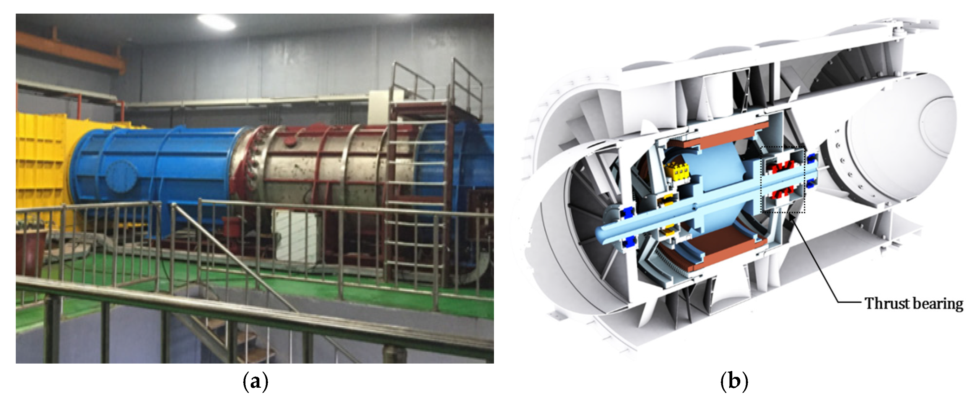
In the OWC WEC, pressure variations produced by water-column oscillation are converted to rotational mechanical power by the impulse turbine (Figure 2) [4,6]. The rotor and blade passages generate alternating aerodynamic forces that are transmitted through the shaft to the bearing assembly [11]. The thrust bearing reacts axial loads arising from asymmetric pressure fields and rotor inertia and therefore plays a central role in the stability and safety of turbine operation [8,9,11]. Repeated excitation leads to wear, increases frictional heating, and can accelerate fatigue of rolling elements and raceways [8,9,10]. A prior failure mode and effects analysis identified the thrust bearing as a high-priority element for condition-based monitoring because accessibility is limited and degradation can progress rapidly under dynamic loading. A site-wide data acquisition system was therefore deployed to track chamber pressure, airflow, turbine rotational speed, bearing temperature, triaxial vibration at the bearing housing, and generated power [11]. Figure 3 provides a close-up of the thrust bearing installed within the turbine assembly.

2.2. Sensor Data Acquisition and Signal Preprocessing

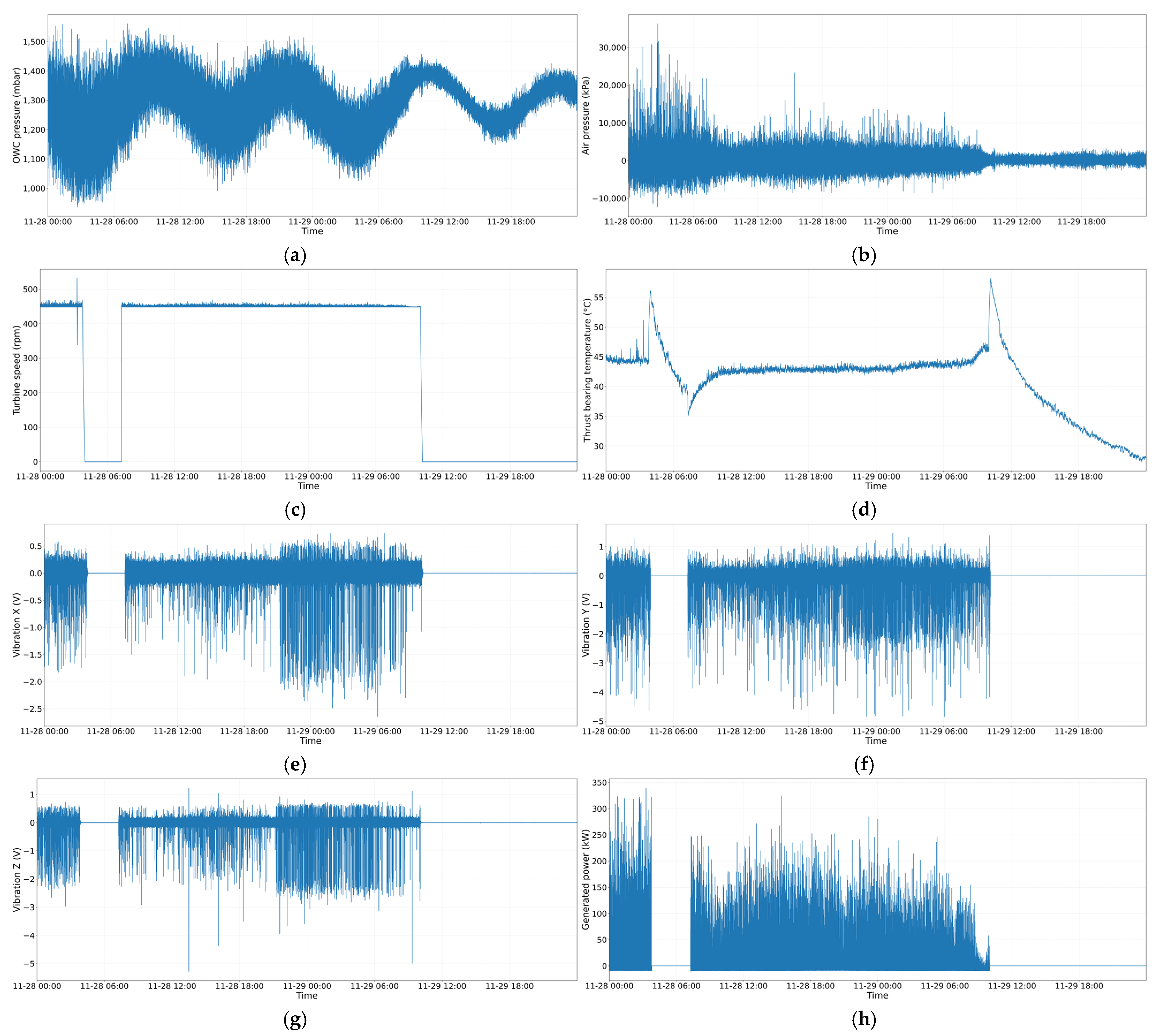
To monitor the marine environment and the operating state of the OWC WEC, a total of 73 sensors are installed, and the supervisory system logs all channels at 20 Hz. Eight channels were selected for detailed analysis because they are most directly associated with turbine operating state and thrust-bearing condition: water-column pressure, air chamber pressure, turbine speed, thrust-bearing temperature, triaxial vibration at the bearing housing along the X, Y, and Z axes, and generated power (

Table 1. Sensor channels and units used to monitor the impulse turbine and thrust bearing in the OWC WEC.

No.	Sensor	Unit	Description
1	OWC pressure	mbar	Static pressure of the oscillating water column
2	Air pressure	kPa	Air chamber pressure inside the turbine system
3	Turbine speed	rpm	Rotational speed of the impulse turbine
4	Temperature	°C	Thrust-bearing temperature
5	Vibration (X axis)	V	X-axis vibration signal on the thrust bearing
6	Vibration (Y axis)	V	Y-axis vibration signal on the thrust bearing
7	Vibration (Z axis)	V	Z-axis vibration signal on the thrust bearing
8	Generated power	kW	Electrical power output

). These channels provide complementary views of hydrodynamic forcing, thermomechanical response, local vibration at the bearing, and electrical output.

Denoised 48 h time histories from 00:00 on 28 November to 00:00 on 30 November 2020 are shown in Figure 4. Water-column and chamber pressures exhibit short-term fluctuations consistent with incident wave groups and wave-climate variability (Figure 4a,b). Turbine speed remains near 440–450 rpm during active operation, with discrete start and stop events driven by operating set points and safety constraints (Figure 4c). Thrust-bearing temperature is typically 40–45 °C under load, with slow drifts attributable to duty cycles and ambient conditions (Figure 4d). Vibration along the X, Y, and Z axes remains within characteristic envelopes in normal service, with amplitude modulation that mirrors turbine duty and the sea state (Figure 4e–g). Generated power follows the activation schedule and exhibits shutdowns when the sea state exceeds predefined limits (Figure 4h) [4,6].

Marine environments introduce transient spikes and telemetry outliers from electrical interference, intermittent contacts, and communication artifacts. To suppress these disturbances while preserving underlying trends, each channel is median filtered with a 20-sample window (1 s at 20 Hz), chosen empirically to balance noise reduction and signal fidelity [10]. Compared with a moving average, the median filter is more robust to isolated spikes and short bursts; it stabilizes the downstream time-domain features and thereby lowers false-alarm propensity when a dynamic threshold is applied to the aggregated reconstruction error [21,22]. After filtering, features are computed every 10 s from the triaxial vibration signals, and an operational status gate derived from speed and power excludes inactive periods from training and detection.

2.3. Correlation Analysis of Sensor Signals

Correlation analysis was performed to characterize statistical relationships among sensor signals and to guide feature selection in the subsequent model design [19,22]. Pearson correlation coefficients were computed on the median-filtered signals over the full 48 h interval. The heat map in Figure 5 shows moderate correlations among the three vibration axes at the bearing housing (approximately 0.48–0.73), between water-column pressure and chamber pressure, and between turbine rotational speed and bearing temperature. Because this global analysis includes intervals when the turbine was not active, operational relationships may be diluted by the inclusion of non-operational periods.

To isolate behavior during turbine operation, a refined analysis was conducted for the 24 h window from 08:00 on 28 November to 08:00 on 29 November 2020 (Figure 6). In this result, rotational speed and generated power exhibit a strong correlation of about 0.95, which reflects direct electromechanical coupling. The three vibration axes correlate with each other in the range of about 0.50–0.75, while their correlation with pressure, speed, and temperature is negligible (below 0.08). This pattern indicates that local mechanical vibration at the bearing housing behaves largely independently of slow variations in hydrodynamic forcing and thermal state once operating periods are isolated, consistent with site observations [11]. Based on these findings, the anomaly-detection methodology in Section 3 focuses on triaxial vibration features as primary inputs.

3. Anomaly-Detection Strategy for Thrust Bearings

This section outlines a data-driven strategy to detect anomalies in the thrust bearing of the impulse turbine under realistic operating variability in an OWC WEC. The approach centers on triaxial vibration measured at the bearing housing and uses an operational status gate to ensure that both training and detection focus on active turbine periods [11,15,20]. Operational status is inferred from rotational speed (rpm) and electrical power, which allows start-up, shutdown, and idling intervals to be excluded from modeling. Limiting the analysis to loaded operation improves sensitivity to subtle load-related deviations. Preprocessing addresses marine transients and telemetry spikes that can inflate feature variance. All channels are median filtered to suppress isolated bursts while preserving step-like operating transitions; the denoised behavior and operating cycles are illustrated in Figure 4. Because supervisory logging is limited to 20 Hz, frequency resolution is insufficient for reliable spectral indicators, and a compact time-domain representation is adopted. At fixed 10 s intervals, six statistical features are extracted from each vibration axis: absolute mean, standard deviation (STD), root mean square (RMS), skewness, shape factor (SF), and crest factor (CF). The triaxial features form an 18-dimensional input vector at each time step.

The predictive core is a feature-based autoencoder that learns the statistical features of normal operation by reconstructing these input vectors. During training, the network estimates a low-dimensional latent representation and minimizes the mean squared error (MSE) between inputs and reconstructions. For anomaly detection, reconstruction errors are computed and aggregated across the six features and three axes to produce a single error time series; larger values indicate greater deviation from the learned normal state.

Operating baselines drift with the sea state, duty cycles, and environmental conditions, so a fixed decision level is inadequate. A dynamic threshold is therefore used. The threshold is updated from a sliding-window estimate of the moving mean and standard deviation of the aggregated reconstruction error, which reduces false positives during slow baseline changes while maintaining sensitivity to genuine anomalies [21,22].

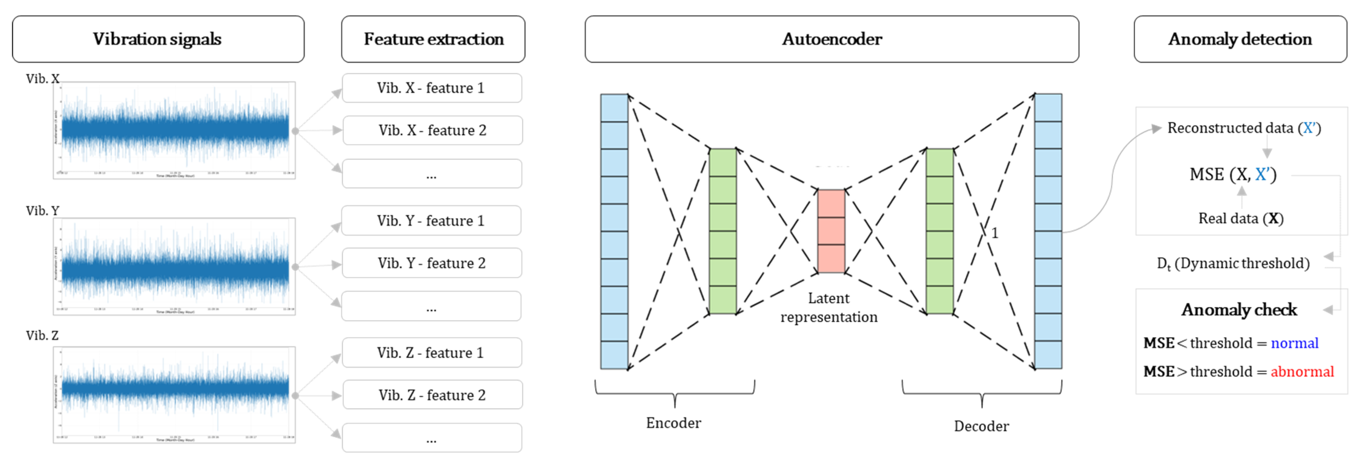
Figure 7 summarizes the complete pipeline. Active operation is identified from rotational speed and power, signals are median filtered, and features are extracted at 10 s resolution. The autoencoder reconstructs the feature vectors, reconstruction errors are aggregated across features and axes, and anomalies are flagged when the aggregated error exceeds the dynamic threshold. Section 3.1 describes the feature rationale and the autoencoder formulation, and Section 3.2 describes the hyperparameter optimization and its effect on reconstruction performance.

3.1. Feature-Based Autoencoder

Selecting informative features is central to anomaly detection at the 20 Hz sampling rate available in the operational OWC WEC. At this rate, frequency-domain indicators are unreliable because only a narrow band of usable content is captured while the turbine rotates near 440–450 rpm. Characteristic bearing tones and sidebands often occur at several multiples of shaft speed and thus fall partly outside the recorded band. Nonstationary sea states further broaden and shift spectral content, which makes spectral estimates coarse and prone to leakage when only 200 samples are available in a 10 s window. For these reasons, time-domain statistics were adopted for their physical interpretability and robustness to marine noise. All channels are denoised with a median filter using a 20-sample window (1 s at 20 Hz) to suppress spikes while preserving operating transitions, which stabilizes vibration features used for condition monitoring [10,11]. Features are then computed every 10 s from triaxial vibration measured at the thrust-bearing housing. Only intervals identified as active operation by the operating-state indicator are used for training and inference so that the learned representation reflects normal behavior under load.

The feature set comprises six time-domain statistics extracted independently from the X-, Y-, and Z-axis signals, yielding an 18-dimensional vector at each time step. AbsMean is sensitive to level shifts associated with looseness and wear. STD quantifies dispersion that grows with broadband excitation. RMS captures signal energy and correlates with load-dependent forcing. SKEW measures waveform asymmetry that can arise from intermittent contact. SF (=RMS/AbsMean) emphasizes waveform sharpness and envelope modulation while reducing sensitivity to slow level drift. CF (= peak/RMS) highlights impulsive peaks linked to localized defects and clearance changes [10,11]. Definitions are provided in

Table 2. Time-domain statistical features extracted from thrust-bearing vibration over the time window and their definitions.

Feature	Definition
Absolute mean (AbsMean)	$AbsMean={\displaystyle \frac{{\sum }_{m-1}^{N}x\left(n\right)}{N}}$
Standard deviation (STD)	$STD=\sqrt{{\displaystyle \frac{{\sum }_{m-1}^N{(x\left(n\right)-Mean)}^2}{N-1}}}$
Root mean square (RMS)	$RMS=\sqrt{{\displaystyle \frac{{\sum }_{m-1}^N{\left(x\left(n\right)\right)}^2}{N}}}$
Skewness (SKEW)	$Skewness={\displaystyle \frac{{\sum }_{m-1}^N{\left(x\left(n\right)-Mean\right)}^3}{\left(N-1\right){\sigma }^3}}$
Shape factor (SF)	$SF={\displaystyle \frac{RMS}{\frac{{\sum }_{m-1}^N\left|x\left(n\right)\right|}{N}}}$
Crest factor (CF)	$CF={\displaystyle \frac{\frac{1}{2}[\max \left(x\left(n\right)\right)-\mathrm{m}\mathrm{i}\mathrm{n}(x\left(n\right)\left)\right]}{RMS}}$

and representative time histories are shown in Figure 8.

The chosen features were evaluated against alternatives under the site constraints. In pilot comparisons within the autoencoder pipeline, kurtosis and peak-to-peak amplitude were considered as additional impulsiveness indicators. At 10 s windows they exhibited higher variance and overlapping distributions, which increased false-alarm propensity. CF provided comparable sensitivity to impulsive events with better stability, so kurtosis and peak-to-peak amplitude were not retained. This supports the selected set as a balanced choice for capturing degradation while maintaining robustness at low sample counts.

Feature selection and justification were guided by the operational constraints and by prior studies [11]. Candidate features were compiled from previous work on this facility and from the diagnostics literature, then screened within an autoencoder-based pipeline using targeted case studies. Screening prioritized three properties. First, reconstruction fidelity on normal data, quantified by mean absolute error (MAE). Second, stability to marine transients after median filtering. Third, separability between normal and simulated-fault windows at 10 s resolution. The resulting six-feature set provided the best balance between sensitivity to degradation and robustness to environmental variability with minimal computational cost [18,19,20].

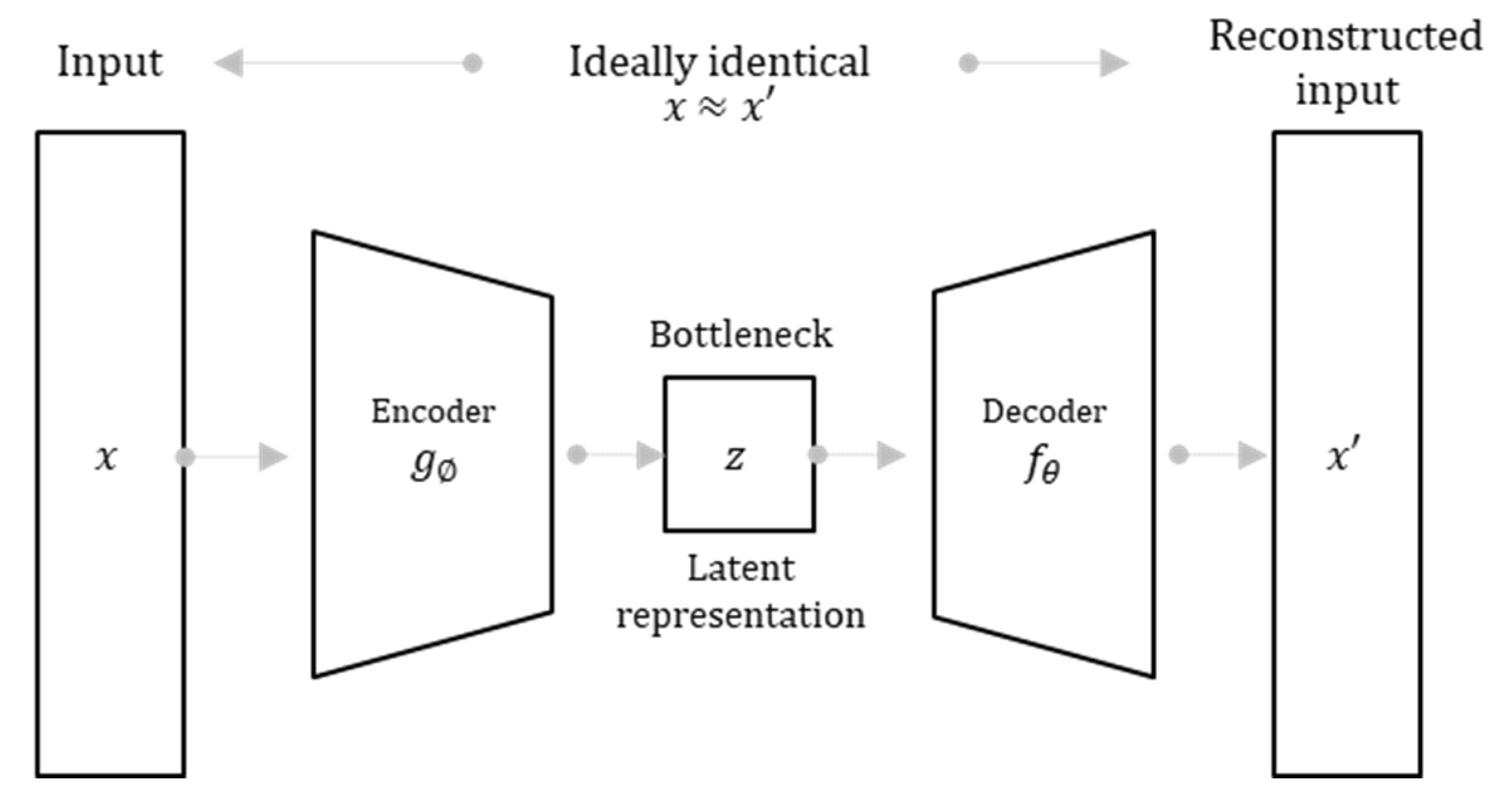
In the autoencoder, the encoder function $g_{\mathrm{\varnothing }}$ compresses the input $x$ into a low-dimensional latent representation $z$ as in Equation (1). The decoder function $f_{\theta }$ maps $z$ back to the feature space to obtain the reconstruction $x^{\prime }$ as in Equation (2). Training minimizes the mean squared error between $x$ and $x^{\prime }$ on data identified as normal, as in Equation (3).

In the autoencoder, the encoder $g_{\mathrm{\varnothing }}$ maps the input feature vector $x$ to a low-dimensional latent representation $z$ (Equation (1)), and the decoder $f_{\theta }$ maps $z$ back to the feature space to obtain the reconstruction $x^{\prime }$ (Equation (2)). Training minimizes the mean squared error between $x$ and $x^{\prime }$ on data identified as normal (Equation (3)).

$$z=g_{\mathrm{\varnothing }}\left(x\right),$$

(1)

$$x^{\prime }=f_{\theta }\left(z\right),$$

(2)

$$L\left(x,x^{\prime }\right)={\displaystyle \frac{1}{D}}{\sum }_{i=1}^D{(x_i-x_i^{\prime })}^2,$$

(3)

where $\theta$ and $\mathrm{\varnothing }$ are the parameters of the encoder and decoder, respectively, and $D$ is the number of features in $x$ (in this study, $D=18$). Optimizing this loss encourages the latent representation to capture the salient structure of normal operation so that departures from normal behavior yield larger reconstruction errors. Figure 9 shows the model architecture and the reconstruction-error workflow.

3.2. Hyperparameter Optimization

Hyperparameters were tuned to improve reconstruction fidelity on normal operation while keeping model capacity modest for field deployment [26,27]. A grid search over fully connected architectures and training settings was conducted, and the best model was selected by minimizing the validation MAE on held-out normal data.

The search space covered encoder and decoder widths, bottleneck size, learning rate, and batch size. Layer widths of 16, 32, and 64 units were tested for the first hidden layer, and 8, 16, and 32 units for the second hidden layer. Bottleneck sizes of 2, 4, 6, and 8 were considered. Learning rates of 1.0 × 10⁻⁴, 2.0 × 10⁻⁴, 5.0 × 10⁻⁴, and 1.0 × 10⁻³ were evaluated with the Adam optimizer, and batch sizes from 32 to 512 were tested. Hidden activations were ELU in the first layer and ReLU in the second; the bottleneck and output layers were linear, and the training loss was MSE. Features were computed at 10 s resolution from median-filtered triaxial vibration during active operation. An 80:20 split on contiguous normal segments provided training and validation sets, and shuffling was disabled to preserve temporal structure.

Table 3. Hyperparameter settings for the feature-based autoencoder: initial configuration and selected values after grid search, with validation MAE before and after optimization.

Hyperparameter	Initial Value	Optimized Value
Neurons in first layer	32	64
Neurons in second layer	16	64
Neurons in third layer	4	8
Learning rate	0.0002	0.001
Batch size	256	64
MAE	0.1935	0.0236

lists the initial configuration and the optimized setting with the associated validation MAE. The selected model uses 64 units in the first hidden layer, 64 units in the second hidden layer, a bottleneck of 8, a learning rate of 0.001, and a batch size of 64. This configuration reduced the validation MAE from 0.1935 to 0.0236, indicating tighter reconstruction of normal feature vectors and clearer separation between normal and abnormal behavior during inference.

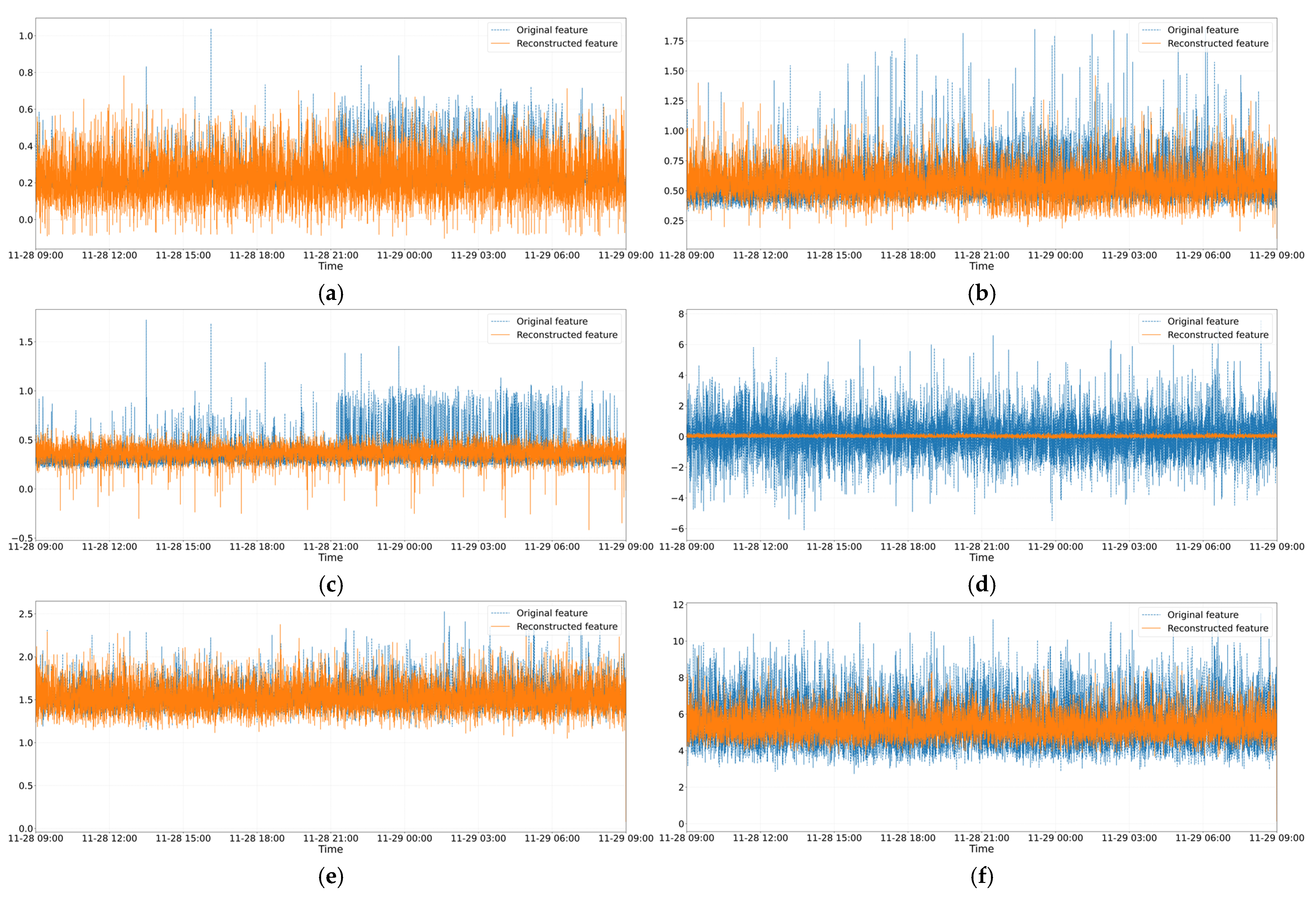
Figure 10 and Figure 11 illustrate the effect on representative X-axis features. Figure 10 shows larger residuals for the initial model, whereas Figure 11 shows closer alignment between input and reconstruction after tuning for AbsMean, STD, RMS, SKEW, SF, and CF. These results confirm that the optimized hyperparameters improve reconstruction fidelity without unnecessary model complexity.

For reproducibility, Table 3 reports the full parameter set and training settings, including validation split, optimizer, activations, and batch size. Random seeds, data splits, and feature definitions are fixed across experiments, and the optimized model is used in subsequent detection and performance evaluation.

4. Anomaly Detection for Impulse Turbine Thrust Bearing

4.1. Validation Using Simulated Fault Data

The anomaly-detection model was evaluated with a two-part protocol combining field measurements and simulated fault scenarios. The autoencoder was trained on a 24 h segment of normal operation, from 08:00 on 28 November to 08:00 on 29 November 2020, during which the impulse turbine operated nominally (see Figure 4). Figure 12 shows the triaxial vibration dataset used to validate the anomaly-detection model, including the 40-min simulated fault window. For testing, a separate 2 h segment from 01:00 to 03:00 on 28 November 2020 was used. This interval reflects representative operating dynamics and environmental variability but contains no documented bearing faults; moreover, confirmed failures are rare in field logs, which limits direct assessment if only natural data are used [7,11,28,29].

To address this limitation, fault-like behavior was simulated following experimental evidence reported by Kim et al. [11], where thrust-bearing degradation produced broadband vibration growth of approximately 200–300 percent relative to baseline due to localized wear, looseness, and imbalance. Consistent with those findings, a 40 min fault window was injected at the end of the 2 h test segment by scaling the raw triaxial vibration signals by a factor of two from 02:20 to 03:00. Scaling was applied before preprocessing and feature computation so that denoising and feature extraction proceeded exactly as in training, preserving temporal structure, cross-axis relationships, and marine-noise characteristics. Figure 13b illustrates the resulting trajectories, which display a clear amplitude increase during the injected window.

Features were computed every 10 s from the median-filtered signals, yielding one 18-dimensional vector per time step. The test set therefore consists of an initial normal portion followed by a fault-like portion. With a 2 h test segment and a 40 min injected window, the sample counts are 480 normal and 241 fault-like observations, for a total of 721 vectors when endpoints are included. This construction provides labeled segments for quantitative evaluation without altering the upstream preprocessing or the feature definitions. Although simulated faults cannot fully capture the nonlinear progression of real bearing damage, they provide a controlled and repeatable basis for initial validation and are commonly employed in condition-monitoring research, especially when safety and rarity limit access to verified failures [15,18,30,31,32,33]. Future work will incorporate empirical fault progressions from extended field monitoring and fusion of virtual and real data to strengthen external validity [33].

4.2. Anomaly Detection Based on Dynamic Thresholding

Vibration from the thrust-bearing housing along the X, Y, and Z axes in the 2 h test segment is processed with the same six time-domain features used in training. AbsMean, STD, RMS, SKEW, SF, and CF are computed every 10 s from median-filtered signals, yielding one 18-dimensional feature vector per time step. The trained autoencoder reconstructs each vector. The reconstruction error at time t is first evaluated component-wise as the squared difference between each input feature and its reconstruction; these errors are then summed across the six features and three axes to form a single error series $e\left(t\right)$. Aggregation improves stability by pooling complementary signatures of degradation and reduces the influence of any single noisy component [19,20].

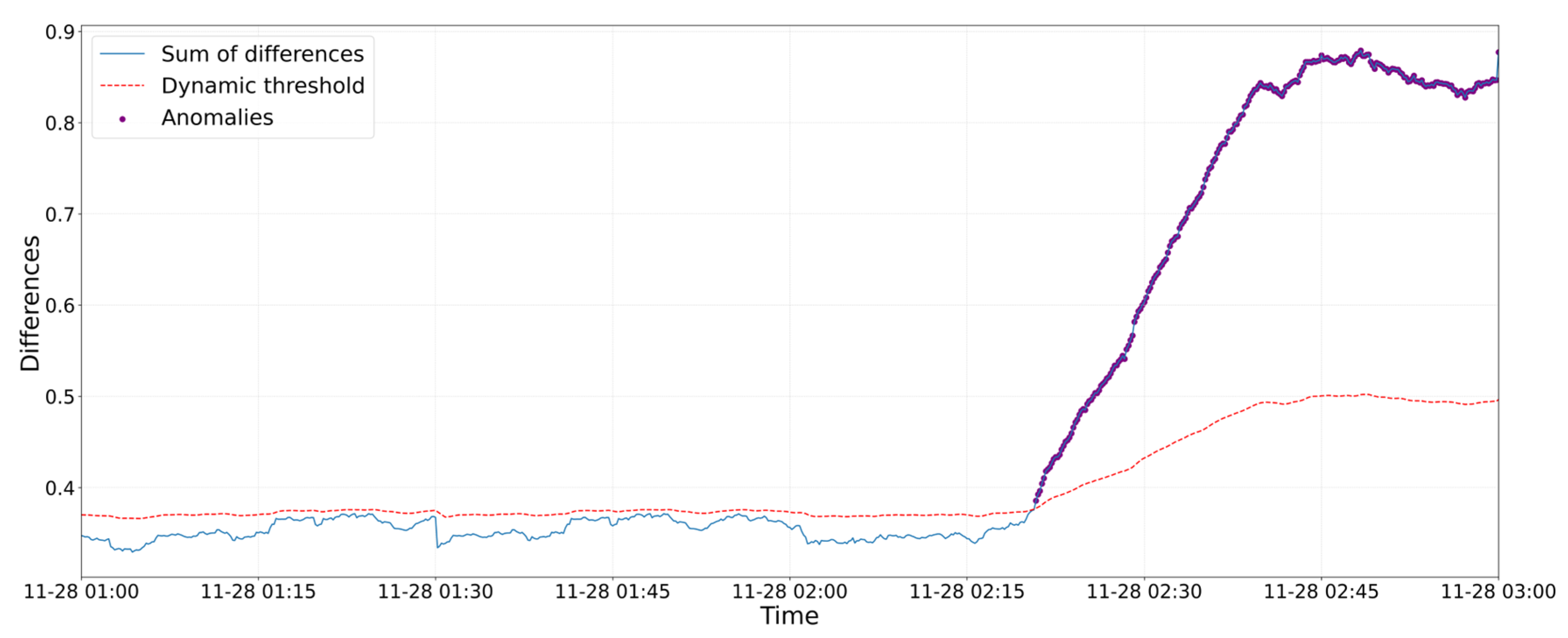
Figure 13a presents the per-feature reconstruction errors, and Figure 14 presents the aggregated error $e\left(t\right)$. During the final 40 min, which corresponds to the injected simulated fault interval, the error magnitude increases clearly and persists. Earlier portions remain near a low baseline with small fluctuations that reflect sea-state variability, duty cycles, and sensor noise. These baseline changes motivate an adaptive decision level rather than a fixed threshold.

A dynamic threshold is applied to the aggregated error. The threshold $\theta \left(t\right)$ is computed from a moving average $\mu \left(t\right)$ and a moving standard deviation $\sigma \left(t\right)$ over a trailing 120 s window:

$$\theta \left(t\right)=\mu \left(t\right)+\alpha ·\sigma \left(t\right),$$

(4)

In this study, $\alpha$ = 2.0 balances sensitivity and false-alarm rate under the observed operating variability. The trailing window is evaluated online so the decision is causal and suitable for field deployment [21,22]. An observation is flagged as anomalous when $e\left(t\right)>\theta \left(t\right)$.

Figure 14 overlays the aggregated error with the dynamic threshold and marks detected anomalies. The threshold follows gradual baseline drift during normal operation and increases during broader variability, yet remains below the elevated error levels within the injected window. This behavior limits false positives when operating points shift and sea state evolves, while maintaining sensitivity for sustained increases in energy and impulsiveness characteristic of thrust-bearing degradation [2,3,21,22].

From an implementation perspective, computation is lightweight. Feature extraction and aggregation use simple statistics at 10 s intervals, and the threshold update needs only the running mean and standard deviation of $e\left(t\right)$ over the most recent 120 s. Detection latency is bound by the window length and the 10 s step, which is compatible with near-real-time monitoring at the site’s 20 Hz logging rate. Parameter values, including the window length and α, are fixed across experiments for reproducibility and match the settings used in the figures.

4.3. Performance Evaluation of the Anomaly-Detection Model

Performance was assessed as a binary classification problem on a 2 h test set that includes a 40 min fault-like window. The detection framework combines a feature-based autoencoder with a dynamic threshold and is evaluated by its ability to classify operating states as normal or anomalous. Quantitative results are accompanied by discussion of reliability, generalizability, and practical applicability to real-world marine energy systems [24,30,34,35,36,37,38,39].

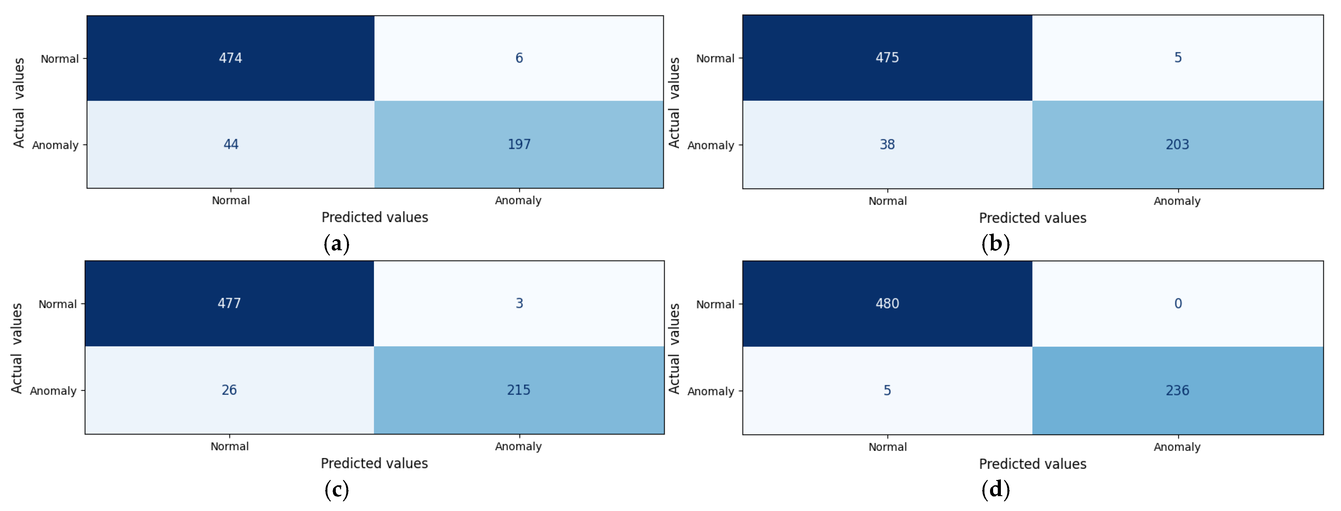
These results indicate strong detection performance. The absence of false alarms is particularly important where unnecessary shutdowns impose economic penalties. The few false negatives occurred near the onset of the injected window, which is consistent with the adjustment delay of the moving average-based dynamic threshold [21,22]. This transient lag does not materially affect early-warning capability because subsequent anomalies were detected promptly.

For completeness, the standard metrics are defined as follows:

$$Accuracy={\displaystyle \frac{TP+TN}{TP+FP+FN+TN}},$$

(5)

$$Precision={\displaystyle \frac{TP}{TP+FP}},$$

(6)

$$Recall={\displaystyle \frac{TP}{TP+FN}},$$

(7)

$$F1 Score=2\times {\displaystyle \frac{Precision\times Recall}{Precision+Recall}},$$

(8)

Figure 15 and

Table 4. Confusion matrix for the 2 h test set (721 samples).

	Predicted Positive	Predicted Negative
Actual positive	TP = 236	FN = 5
Actual negative	FP = 0	TN = 480

present the confusion matrix computed from 721 feature vectors sampled at 10 s intervals. Of these, 480 correspond to normal operation and 236 to abnormal states created by doubling the triaxial vibration amplitudes during the final 40 min. The detector correctly labeled all 480 normal samples as true negatives (TN = 480) and identified 236 of the 241 abnormal samples as true positives. Five abnormal samples were missed as false negatives (FN = 5), and there were no false positives (FP = 0).

To assess relative performance, four anomaly-detection models were implemented on the same 2 h test set. First, fixed thresholding set a decision level from statistics of the normal portion of the test data and classified samples using the scalar energy of the feature vector at each time step, ‖x‖². Second, the PCA reconstruction method standardized the normal reference segment, retained principal components up to a chosen cumulative explained variance, and used a threshold on the reconstruction error. Third, the LSTM autoencoder trained 12-step sequences (about 2 min) on normal data and used the sequence-averaged MSE as the anomaly score. Finally, the proposed approach uses an 18-dimensional time-domain feature vector from triaxial vibration, comprising AbsMean, STD, RMS, SKEW, SF, and CF, together with a dynamic threshold computed from a sliding-window mean and standard deviation.

Table 5. Performance metrics on the 2 h test set (721 samples; last 40 min include simulated faults).

Method	Accuracy	Precision	Recall	F1 Score
Fixed thresholding	0.93	0.97	0.82	0.89
PCA reconstruction	0.94	0.98	0.84	0.90
LSTM	0.96	0.99	0.89	0.94
Proposed method	0.99	1.00	0.98	0.99

summarizes the results. The proposed method achieved the highest scores with accuracy of 0.99, precision of 1.00, recall of 0.98, and F1 score of 0.99, and it produced zero false positives, which is advantageous for field deployment [37,38,39]. The LSTM autoencoder ranked second by leveraging temporal dependence; PCA reconstruction was comparatively robust to noise and consistently outperformed fixed thresholding; and fixed thresholding, while simple to implement, was more sensitive to baseline shifts such as sea state and duty changes. Figure 15 presents the confusion matrices for all four methods.

From an application perspective, three aspects support deployment. First, the method operates reliably with 20 Hz signals and compact time-domain features, aligning with common constraints in field installations. Second, aggregation of reconstruction errors across the six features and three axes yields a stable indicator that remains sensitive to progressive degradation while attenuating incidental fluctuations. Third, the dynamic threshold adapts to slow baseline drift, enabling conservative decisions under variable sea states. Together, these properties support condition-based monitoring and early fault detection for the thrust bearing in OWC WECs [7,11,19,21]. In the results, the combination of physically motivated features and adaptive thresholding explains the zero false-alarm rate and high recall: the features capture energy growth and impulsiveness linked to degradation, while the threshold tracks operating drift without masking sustained deviations. By contrast, fixed thresholds lacked adaptability, PCA was limited by linear reconstruction, and LSTM incurred greater complexity for a smaller gain. These trade-offs indicate that the proposed approach provides the most favorable balance of sensitivity, robustness, and computational cost for 20 Hz supervisory data.

5. Conclusions

A data-driven anomaly-detection framework was developed and validated for the thrust bearing of the impulse turbine in an OWC WEC using field data from an operational 500 kW class facility. A failure mode and effects analysis identified the thrust bearing as a priority for condition-based monitoring. Among sensors sampled at 20 Hz, eight channels were selected for analysis, and correlation results showed that triaxial vibration measured at the bearing housing provides the most direct indicator for anomaly detection.

The approach employs a feature-based autoencoder trained on 24 h of normal operation with six time-domain statistical features from the vibration signals of X, Y, and Zaxes. Median filtering stabilizes inputs in the presence of marine noise and telemetry spikes, and operational status screening removes non-operational intervals, so the learned representation reflects true load conditions. Anomaly decisions use a dynamic threshold computed from the moving mean and standard deviation of the aggregated reconstruction error, which adapts to slow baseline drift. Hyperparameter optimization by grid search improved reconstruction fidelity on validation data, reducing mean absolute error from 0.1935 to 0.0236.

Performance on a 2 h test set with a 40 min simulated-fault interval yielded a confusion matrix of TN = 480, FP = 0, FN = 5, and TP = 236, corresponding to accuracy of 0.99, precision of 1.00, recall of 0.98, and F1 score of 0.99. In addition, benchmark comparisons on the same test set showed that the proposed method outperformed fixed thresholding, PCA reconstruction, and an LSTM, achieving the highest accuracy and F1 score and producing zero false positives, which is advantageous for field deployment. The absence of false positives mitigates the risk of unnecessary alarms in practical deployment, and the small number of early false negatives is consistent with the adjustment delay of a moving-window threshold and did not hinder subsequent detection. These outcomes indicate dependable detection at low sampling rates with modest computational load.

The design choices are grounded in physical reasoning. The selected time-domain features summarize energy, dispersion, asymmetry, and impulsiveness linked to bearing degradation, and the denoising step improves indicator stability and threshold robustness under environmental variability. The framework is transparent, uses compact inputs, and is suitable for on-site implementation, which supports condition-based monitoring and early fault indication in OWC WECs. Limitations remain because verified bearing faults are scarce in field logs and part of the evaluation uses simulated-fault scenarios. Future work will emphasize long-term monitoring with empirically observed fault progressions, validation across multiple sites and hardware configurations, collaboration with OWC operators, integration with digital-twin workflows and reliability-centered maintenance, adaptive tuning of threshold parameters, uncertainty quantification for decision support, and extensions to other rotating components within the OWC WEC drivetrain.