Article

Multi-Point Seawall Settlement Modeling Using DTW-Based Hierarchical Clustering and AJSO-LSTM Method

1
School of Hydraulic Engineering, Zhejiang University of Water Resources and Electric Power, Hangzhou 310018, China
2
Department of Civil and Environmental Engineering, The Hong Kong University of Science and Technology, Hong Kong 999077, China
3
School of Civil Engineering, Sun Yat-sen University, Zhuhai 519082, China
*
Author to whom correspondence should be addressed.
J. Mar. Sci. Eng. 2025, 13(11), 2053; https://doi.org/10.3390/jmse13112053
Submission received: 27 September 2025 / Revised: 19 October 2025 / Accepted: 23 October 2025 / Published: 27 October 2025

Abstract

A seawall settlement is a critical concern in marine engineering, as an excessive or uneven settlement can undermine structural stability and diminish the capacity to withstand marine hydrodynamic actions such as storm surges, waves, and tides. Accordingly, accurate settlement prediction is vital to ensuring seawall safety. To address the lack of clustering methods that capture the time-series characteristics of monitoring points and the limitations of hyperparameter sensitivity of conventional LSTM models, this study proposes a hybrid model integrating Dynamic Time Warping-based Hierarchical Clustering (DTW-HC) and an Adaptive Joint Search Optimization-enhanced Long Short-Term Memory Model (AJSO-LSTM). First, DTW-HC is employed to cluster monitoring points according to their time series characteristics, thereby constructing a spatial panel data structure that incorporates both temporal evolution and spatial heterogeneity. Then, an AJSO-LSTM model is developed within each cluster to capture temporal dependencies and improve prediction performance by overcoming the weaknesses of a conventional LSTM. Finally, using seawall settlement monitoring data from a real engineering case, the proposed method is validated by comparing it with a statistical model, a back-propagation Neural Network (BP-ANN), and a conventional LSTM. Results demonstrate that the proposed model consistently outperforms these three benchmark methods in terms of prediction accuracy and robustness. This confirms the potential of the proposed framework as an effective tool for seawall safety management and long-term service evaluation.

1. Introduction

A seawall settlement is a critical issue in marine and coastal engineering, as an excessive or uneven settlement can compromise structural stability and diminish a seawall’s capacity to protect coastal areas from storm surges and tidal flooding [1,2,3]. Accordingly, monitoring-driven evaluation that leverages multi-point structure monitoring observations and time-series analysis is essential for the accurate assessment of settlement behaviors, underpinning safety management and the long-term serviceability of seawalls [4,5,6].
Various approaches have been employed to investigate seawall settlement, including theoretical analysis, numerical simulation, and laboratory or field experiments [7,8,9,10,11,12,13]. These methods have greatly advanced the understanding of the mechanisms of seawall deformation and failure. However, due to the complexity of soil–structure–water interactions and site-specific conditions, the results of theoretical and experimental studies are often difficult to generalize to real projects. In practice, continuous monitoring has become the most reliable way to capture the actual settlement behaviors of seawalls under long-term service conditions [14,15]. Consequently, the prediction of seawall settlement monitoring data has emerged as a key issue in both engineering management and scientific research.
To analyze monitoring data, traditional approaches often rely on statistical models, which establish relationships between historical settlement records and environmental variables such as temperature, time, and water level [16,17,18]. With the rapid development of machine learning, more advanced algorithms, including tree-based methods and neural network based methods, have been introduced to improve prediction performance in many fields [19,20,21,22,23,24,25]. Specifically, deep learning methods have been increasingly adopted for data prediction in hydraulic engineering and structural health monitoring [26,27,28,29]. Additionally, the use of machine learning for fully automated operational modal analysis has seen promising advancements, such as an approach by Mugnaini et al. (2022), which proposes a machine learning-based method with hierarchical clustering, further enhancing predictive capabilities in structural monitoring [30]. Recent studies have pushed spatio-temporal learning along complementary fronts, including GNN-based models that encode sensor topology and temporal regularities for structural monitoring [31], deep-learning approaches that model instrumentation and measurement errors to strengthen end-to-end monitoring reliability [32], and physics-informed spatio-temporal networks that embed governing constraints for improved data efficiency and physical consistency in subsurface and geomechanics applications [33]. These advances are complementary to our monitoring-first, small-data setting with asynchronous dynamics; we leverage DTW–HC to reveal cross-point temporal heterogeneity and AJSO–LSTM to co-tune window length and capacity under practical compute budgets, while remaining compatible with future cluster-wise GNN/Transformer backbones or physics-guided objectives.
The Long Short-Term Memory (LSTM) network has been widely used due to its strong ability to capture temporal dependencies in nonlinear time series. For instance, Qu et al. (2019) developed an RS-LSTM model for concrete dam deformation prediction and demonstrated its superior performance compared with traditional models [34]. Building on this, Li et al. (2020) proposed a stacked LSTM framework combined with Seasonal-Trend decomposition (STL) and extra-trees to enhance displacement prediction accuracy [35]. Later, Li et al. (2022) introduced a dual-stage deep learning model (DRLSTM) directly driven by raw monitoring data, which improved both feature representation and forecasting robustness [27]. More recently, Madiniyeti et al. (2023) developed an SSA–LSTM model that integrates Singular Spectrum Analysis to better extract temporal components from monitoring data [36]. Zheng et al. (2023) developed a CPSO-WNN-LSTM model for seawall deformation prediction, demonstrating the effectiveness of combining optimization algorithms with LSTM-based frameworks [37]. Although these improved LSTM-based methods have achieved notable progress, they still face certain limitations. Specifically, the predictive performance is highly sensitive to hyperparameter tuning, the optimization processes may easily fall into local optima, and model adaptability to diverse monitoring datasets remains limited. To address these issues, we employ Adaptive Joint Search Optimization (AJSO) as an outer-loop, population-based optimiser that jointly searches the end-to-end pipeline—window length (daily sampling), normalisation choice, model capacity, batch size, and learning rate—while weights are still learned by Adam in the inner loop. Unlike approaches that tune a narrow subset of hyperparameters or embed meta-heuristics directly into weight updates, AJSO optimises a horizon-aware multi-step validation loss under chronological blocking, with all transforms fitted on train only to avoid leakage. Its controlled exploration–exploitation schedules and fixed population improve reproducibility, reduce the risk of local optima, and yield configurations that generalise more robustly across heterogeneous monitoring sites.
Traditional prediction approaches usually establish models for a single monitoring point, without considering spatial correlation. To improve this, multi-point panel data models have been developed that exploit spatial–temporal data [38,39]. For instance, Li et al. (2021) proposed a multiple-monitoring-point prediction framework for rockfill dams, which significantly enhanced the accuracy and reliability of settlement prediction at failure points [40]. These studies highlight the importance of incorporating information from multiple monitoring points to improve model robustness. To further account for spatial correlation, clustering-based strategies have been proposed. For example, Fattahi and Bayatzadehfard (2018) applied clustering methods in combination with ANN-BBO and ANFIS models to forecast tunneling-induced surface settlement [41]. More recently, Beiranvand et al. (2024) developed an AI model that integrates spatiotemporal clustering with the k-means algorithm for predicting earth dam settlement, confirming the potential of clustering in enhancing prediction performance [42]. Nevertheless, most clustering criteria are still based on static point attributes (e.g., distance to dam/seawall crest, convergence ratio, aging sequence, etc), which fail to capture the dynamic evolution of settlement at different locations [43,44,45]. To address this gap, we focus on clustering monitoring points according to their time series characteristics, thereby upgrading traditional panel data analysis into spatial panel data analysis, so as to enable the joint utilization of temporal patterns and spatial heterogeneity.
This study aims to solve two key problems in seawall settlement prediction: (i) the lack of clustering methods that capture time series characteristics of monitoring points, and (ii) the limitations of conventional LSTM models, which often suffer from hyperparameter sensitivity, risk of local optima, and insufficient adaptability to complex monitoring datasets. By integrating Dynamic Time Warping–based Hierarchical Clustering (DTW-HC) with AJSO-enhanced LSTM, the proposed framework addresses both issues to achieve more reliable classification and more accurate prediction. First, DTW-HC is employed to group monitoring points with similar temporal evolution, thereby accounting for the spatial heterogeneity of monitoring locations [46,47,48]. Then, for each cluster, an AJSO-LSTM model is developed to capture the temporal dependencies of the panel data and provide accurate predictions [49,50,51,52]. Finally, using seawall settlement monitoring data from a real engineering case, the effectiveness of the proposed model is validated through comparative experiments against a statistical model, a Back-propagation neural network (BP-ANN), and a conventional LSTM.
This article is organized as follows. Section 2 presents the methodology, which consists of two parts: (i) time series data clustering based on DTW-HC, and (ii) AJSO-LSTM prediction applied to each cluster. Section 3 describes the engineering case, including the layout of monitoring points and the characteristics of the monitoring data. Section 4 reports the clustering outcomes as well as the prediction results. Section 5 provides a discussion on the advantages and limitations of the proposed approach, together with potential directions for future research. Finally, concluding remarks are summarized in Section 6.

2. Methods

2.1. Spatial Panel Data Structure

In the study of seawall settlement monitoring, scholars have traditionally relied on two fundamental types of data: cross-sectional data and time-series data. Cross-sectional data refer to settlement observations of multiple monitoring points at a specific time, which can reflect the overall settlement distribution of the seawall at that moment. In contrast, time-series data represent the settlement observations of a single monitoring point across consecutive time steps, thereby capturing its dynamic evolution (see Figure 1). However, relying solely on cross-sectional data makes it difficult to reveal the long-term evolution process, while using only time-series data fails to provide an overall spatial description of the structure. Hence, either type alone is insufficient to fully support the analysis and prediction of seawall settlement behavior.
Panel data combine both cross-sectional and time-series dimensions, enabling systematic recording of multiple monitoring points across different time periods. The corresponding data structure is presented in Table 1. This bidimensional data framework not only reflects the temporal evolution of each monitoring point but also reveals the collective characteristics of the entire system. Consequently, panel data significantly improve the precision of dynamic behavior analysis and the robustness of estimation, making them an important tool in structural settlement studies.
Nevertheless, conventional panel data models remain limited by their assumption of independence among monitoring points, thereby neglecting spatial correlations. In practical seawall engineering, settlement is typically influenced by combined factors such as soil compressibility, groundwater fluctuations, tidal variations, and wave loading. These external effects often induce strong spatial dependencies among adjacent monitoring points. Ignoring such spatial effects may lead to biased estimations and reduced predictive accuracy. By incorporating spatial coordinates or adjacency relationships into the conventional panel framework, spatial panel data are able to simultaneously characterize temporal dynamics, spatial distribution, and spatial dependence effects. The structural representation of spatial panel data is shown in Table 2. Each monitoring point is associated with spatial coordinates ( x i , y i , z i ) , and  δ j ( x i , y i , z i ) denotes the settlement value of point i at time j.
Compared with traditional panel data, spatial panel data provide a more realistic depiction of the spatiotemporal settlement behavior of seawalls, thereby enhancing anomaly detection, local settlement pattern analysis, and overall safety assessment. The hierarchical relation among different data structures is summarized in Figure 2. This study adopts spatial panel data as the fundamental framework for seawall settlement monitoring and prediction.

2.2. AJSO-Optimized LSTM Model

Based on the features of panel data, the settlement monitoring model based on multi-monitoring points is established. Equation (1) expresses the regression coefficients of a panel data, which represents the multi-point settlement panel data model:
δ i t = k = 1 K β k i x k i t + u i t ,
where δ i t denotes the settlement at point i and time t; x k i t denotes the k-th input covariate for point i at time t; t , i denote the time and cross-section indices, respectively; k indexes input variables; β k i are point-specific coefficients; u i t is a random disturbance term.
To capture the nonlinear spatiotemporal dependencies in seawall settlement data, we further construct a nonlinear prediction model based on spatial panel data, namely the AJSO–LSTM model, building upon the linear representation of Equation (1). Figure 3 illustrates the principle of the LSTM method.
Assume the seawall has n monitoring points and observation times t = 1 , , T , with settlement denoted by δ i , t . We first construct a global distance–decay spatial weight matrix W = [ w i j ] n × n ( w i j 0 , w i i = 0 ). For pairs with Euclidean distance d i j r ,
w i j = exp d i j / h , w i i = 0 ,
and w i j = 0 otherwise. Rows are standardized so that j w i j = 1 . The radius r and bandwidth h are selected by validation grid search (train-only) to avoid leakage.
(1)
Neighborhood scope (cluster-wise masking).
Because prediction models are trained per cluster, we restrict spatial interactions to in-cluster neighbors by masking the global weights:
W ( c ) = W M ( c ) , M i j ( c ) = { i S c , j S c } ,
where S c is the index set of points in cluster c and ⊙ denotes the Hadamard product. Rows of W ( c ) are re-standardized so that j w i j ( c ) = 1 for i S c . The spatial lag at time t is then defined (for i S c ) as
s i , t = j = 1 n w i j ( c ) δ j , t ,
which uses the same distance cut-off r and bandwidth h as the global W but masks out cross-cluster neighbors.
To jointly exploit temporal windows and spatial neighborhood information, the LSTM input for point i at time t is
z i , t = δ i , t , s i , t , x i , t R d ,
where x i , t = [ x 1 i t , , x K i t ] collects external drivers (cf. Equation (1)), such as tidal level, temperature, groundwater table, or wave statistics. Given a window length L, the input sequence is
Z i , t ( L ) = z i , t L + 1 , , z i , t .
(2)
Explicit output mapping of δ in LSTM (single-step/multi-step).
Let Θ denote all trainable parameters of the LSTM (weights and biases). The standard gated updates are
f t = σ W f [ h t 1 , x t ] + b f ,
i t = σ W i [ h t 1 , x t ] + b i ,
C ˜ t = tanh W c [ h t 1 , x t ] + b c ,
C t = f t C t 1 + i t C ˜ t ,
o t = σ W o [ h t 1 , x t ] + b o ,
h t = o t tanh ( C t ) ,
where here x t z i , t . A linear output layer maps the hidden state to the settlement prediction:
δ ^ i , t + 1 = W y h t + b y .
For H-step ahead prediction, either recursive or direct multi-output strategies can be adopted:
δ ^ i , t + 1 : t + H = g Θ Z i , t ( L ) = δ ^ i , t + 1 , , δ ^ i , t + H .
(3)
Multi-point joint (MIMO) output within clusters.
Based on the DTW-HC clustering results, let S c denote the set of monitoring points in cluster c. A multi-input multi-output (MIMO) settlement prediction model is then constructed as
δ ^ S c , t + 1 = G Θ c Z i , t ( L ) i S c R | S c | ,
where Θ c are the LSTM parameters for cluster c.
(4)
Training loss (explicitly including δ ) with spatial regularization.
Given the training index set D tr , a weighted MSE loss with spatial smoothness regularization (using W to constrain prediction differences among neighboring points) is defined as
L train ( Θ η ) = 1 | D tr | ( i , t ) D tr ( δ ^ i , t + 1 δ i , t + 1 ) 2 + λ s t i < j w ij ( c ) ( δ ^ i , t + 1 δ ^ j , t + 1 ) 2 + λ 2 Θ 2 2 ,
where η denotes the set of hyperparameters (learning rate, hidden units, number of layers, window L, batch size, etc.), λ s is the spatial regularization coefficient, and  λ 2 is the L 2 regularization weight. We tune λ s on a validation set over { 0 , 10 4 , 10 3 , 10 2 } and select the value minimizing validation error. The selected λ s = < value > (if λ s = 0 , the spatial term is inactive). For multi-step prediction, the error is accumulated across h = 1 , , H in Equation (13).
(5)
δ -driven fitness function and AJSO update.
To optimize hyperparameters with respect to settlement prediction performance, the fitness on the validation set (to be minimized) is defined as
J ( η ) = 1 | D val | ( i , t ) D val δ ^ i , t + 1 ( η ) δ i , t + 1 2 ,
where δ ^ i , t + 1 ( η ) is the prediction under hyperparameters η after training with Equation (15). AJSO searches the hyperparameter space to minimize Equation (16). Let η ( g ) denote a candidate solution at generation g. Its updated rule is
η ( g + 1 ) = η ( g ) + α ( g ) ω ( g ) η η ( g ) + 1 ω ( g ) η ( rand ) η ( g ) ,
where η = arg   min η   J ( η ) is the current global best, η ( rand ) is a randomly selected candidate, α ( g ) is the adaptive step size, and ω ( g ) [ 0 , 1 ] balances global exploration and local exploitation.
We set the AJSO population size to P = 20 and the number of generations to G = 60 . Early stopping if no validation improvement for 20 consecutive generations. Consistent with Equation (17), the adaptive step size α ( g ) decays and the exploration–exploitation weight ω ( g ) [ 0 , 1 ] increases with generation g = 0 , , G :
α ( g ) = α min + ( α max α min ) 1 g G γ , ω ( g ) = ω min + ( ω max ω min ) g G β ,
where α max = 0.9 , α min = 0.1 , ω max = 0.9 , ω min = 0.2 , and  γ = β = 1 .
Through Equation (16), the fitness explicitly depends on the settlement error ( δ ^ δ ) , thus directly incorporating δ into the optimization target.
(6)
Prediction and evaluation.
For the test set ( i , t ) D te , the predictions δ ^ i , t + h ( h = 1 or 1 : H ) are obtained using Equation (12) or Equation (13). Performance is evaluated using RMSE, MAE, R 2 , and—if spatial regularization is applied—the spatial consistency error i < j w i j ( c ) ( δ ^ i , t δ ^ j , t ) 2 .
Table 3 reports the AJSO-selected configurations per cluster: window length (days) L, Sakoe–Chiba band (days) w, distance cutoff r, decay bandwidth h, spatial smoothness weight λ s , soft-DTW smoothing for Ward γ sDTW .
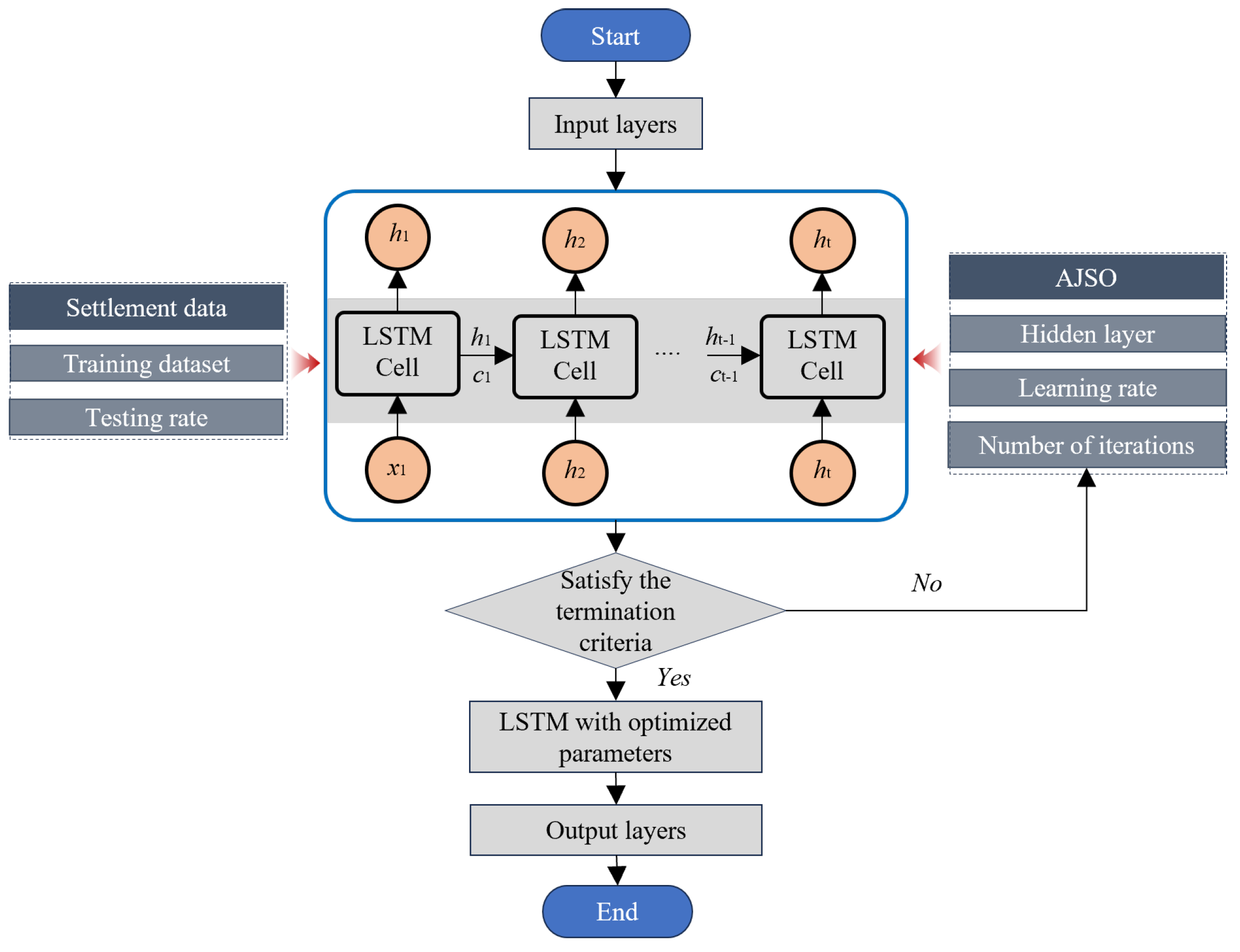
The overall AJSO–LSTM framework is shown in Figure 4. All tuning is performed on the training window only; the test window is used once for held-out evaluation and inherits the train clustering. This in-cluster masking is a conscious modeling choice to prevent cross-regime borrowing and to enhance the interpretability of cluster-wise predictors.

2.3. Data Clustering Based on Time-Series Characteristics Using DTW-HC

To exploit the intrinsic temporal dynamics of seawall settlement data, we adopted a clustering approach based on Dynamic Time Warping (DTW) in conjunction with hierarchical clustering (HC).
Note that we adopt chronological blocking (80/20): T tr = { 1 , , T tr } , T te = { T tr + 1 , , T } . Per-series z-normalization ( μ i , σ i ) is fitted on T tr and applied unchanged to both sets. Pairwise DTW distances and the agglomerative dendrogram are computed on T tr only. After selecting K on the train, each series receives a fixed cluster label c ( i ) , which is inherited by the test window. All hyperparameters are tuned within T tr using inner chronological validation; T te is used once for held-out evaluation.
Let the settlement sequences at monitoring points i and j be
δ i = { δ i , 1 , δ i , 2 , , δ i , T } , δ j = { δ j , 1 , δ j , 2 , , δ j , T } .
The local alignment cost between time indices t and s is defined as
c ( t , s ) = | δ i , t δ j , s | 2 .
The DTW cumulative distance matrix D ( t , s ) is recursively computed by
D ( t , s ) = c ( t , s ) + min D ( t 1 , s ) , D ( t , s 1 ) , D ( t 1 , s 1 ) ,
with initialization D ( 1 , 1 ) = c ( 1 , 1 ) .
The DTW distance between the two sequences is obtained as
D DTW ( i , j ) = D ( T , T ) .
Once the pairwise DTW distance matrix
D = D DTW ( i , j )
is constructed for all monitoring points, and agglomerative hierarchical clustering is applied. The linkage criterion is based on Ward’s method. Since DTW is a non-Euclidean distance, we use soft-DTW to instantiate Ward linkage for within-cluster distance computation. The  γ parameter in soft-DTW controls the smoothness of the time-series alignment: a larger γ allows more flexibility in the alignment, while a smaller γ forces a stricter alignment, similar to traditional DTW. The optimal value of γ is determined through grid search to ensure effective clustering performance.
For a cluster C with time series { x i } i C and soft-DTW cost sDTW γ ( · , · ) , the barycenter is computed by minimizing the soft-DTW distance between the series and the barycenter:
μ C = arg min z i C sDTW γ ( x i , z ) .
The soft-DTW within-cluster sum of squares is
WCSS γ ( C ) = i C sDTW γ ( x i , μ C ) .
At each agglomerative step, we merge the pair ( A , B ) that minimizes the increase in soft-DTW within-cluster sum of squares:
Δ γ ( A , B ) = WCSS γ ( A B ) WCSS γ ( A ) WCSS γ ( B ) .
The barycenter for A B is re-estimated at each merge. Finally, the dendrogram is cut at an empirically determined level, resulting in three major clusters. These clusters represent monitoring points with similar settlement trajectories, thereby enabling subsequent cluster-wise AJSO-LSTM prediction models. This hybrid framework ensures that both time-series alignment and spatiotemporal predictive modeling are effectively leveraged. Figure 5 illustrates the flow chart of the DTW-HC clustering method.

2.4. Algorithm

Algorithm 1 presents the programming procedure of the DTW-HC clustering and AJSO-LSTM prediction. First, settlement sequences from all monitoring points are preprocessed, followed by pairwise similarity calculation using DTW. Local alignment costs are accumulated via dynamic programming, and the resulting DTW distance matrix is subjected to agglomerative HC with Ward’s linkage. Within each cluster, settlement prediction is carried out using AJSO–LSTM. Input features combine raw settlement, spatially lagged values from the spatial weight matrix, and external factors. The AJSO algorithm adaptively tunes LSTM hyperparameters based on validation errors.
Algorithm 1 DTW-based hierarchical clustering and cluster-wise AJSO–LSTM prediction
Require: 
Settlement time series { δ i } i = 1 n with δ i = { δ i , 1 , , δ i , T } ; external factors { x i , t } ; global distance-decay weight matrix W = [ w i j ] (row-standardized); candidate clusters K ; AJSO max generations G, population size P.
Ensure: 
Cluster partition { C 1 , , C K } ; cluster-wise AJSO–LSTM predictions { δ ^ i , t + h } .
  1:
Chronological split (80/20). Define T tr = { 1 , , T tr } and T te = { T tr + 1 , , T } .
  2:
Train-only normalization. Fit per-series z-normalization ( μ i , σ i ) on T tr ; apply the same parameters to all t T tr T te .
  3:
Data preprocessing: handle missing values, resample, detrend/difference (all fitting steps restricted to T tr ).
  4:
(Optional) Set a Sakoe–Chiba band of width w for DTW.
  5:
DTW on train only. Compute pairwise DTW distance matrix D using { δ ˜ i , t } t T tr :
  6:
for  i = 1 to n do
  7:
   for  j = i to n do
  8:
     Define c ( t , s ) = | δ ˜ i , t δ ˜ j , s | 2 and D ( t , s ) = c ( t , s ) + min { D ( t 1 , s ) , D ( t , s 1 ) , D ( t 1 , s 1 ) } .
  9:
     Set D DTW ( i , j ) = D ( T tr , T tr ) and D i j = D j i .
10:
   end for
11:
end for
12:
Clustering on train only. Perform agglomerative HC (Ward/soft-DTW) on D ; select K on T tr ; obtain train clusters { C 1 , , C K } with index sets { S 1 , , S K } .
13:
Fix labels for test. Assign each series a label c ( i ) from train; the test window inherits  c ( i ) (no reclustering on T te ).
14:
In-cluster masked weights. For each cluster c = 1 , , K , form W ( c ) = W M ( c ) with M i j ( c ) = { i S c , j S c } , and row-standardize W ( c ) so that j w i j ( c ) = 1 for i S c .
15:
For each cluster C k (points S k ):
16:
for  k = 1 to K do
17:
   For i S k , set s i , t = j = 1 n w i j ( k ) δ ˜ j , t , z i , t = [ δ ˜ i , t , s i , t , x i , t ] , and  Z i , t ( L ) = ( z i , t L + 1 , , z i , t ) .
18:
   Initialize P candidate hyperparameters { η p ( 0 ) } p = 1 P .
19:
   for  g = 0 to G 1  do
20:
     for  p = 1 to P do
21:
        Train on train only. Train LSTM with η p ( g ) (Adam) on ( i , t ) T tr , minimizing
22:
            L = 1 | D tr | ( i , t ) ( δ ^ i , t + 1 δ ˜ i , t + 1 ) 2 + λ s t i < j w i j ( k ) ( δ ^ i , t + 1 δ ^ j , t + 1 ) 2 + λ 2 Θ 2 2 ,
23:
        where the spatial smoothness uses the same scope W ( k ) .
24:
        Validation inside train. Evaluate fitness on an inner chronological validation
       split within T tr : J ( η p ( g ) ) = 1 | D val | ( i , t ) δ ^ i , t + 1 ( η p ( g ) ) δ ˜ i , t + 1 2 .
25:
     end for
26:
     Update candidates via AJSO: η p ( g + 1 ) = η p ( g ) + α ( g ) ω ( g ) ( η η p ( g ) ) + ( 1 ω ( g ) ) ( η ( rand ) η p ( g ) ) with η = arg min J ( η ) .
27:
   end for
28:
   Train the final LSTM with η on T tr and obtain δ ^ i , t + h (single- or multi-step).
29:
   Held-out test. Evaluate once on T te using the fixed c ( i ) and the same transforms.
30:
end for
31:
Return cluster assignments and prediction results.

3. Case Study

The engineering case is located at a test section of the seawall in Zhejiang Province, China. The foundation soils are characterized by soft marine deposits with high compressibility and low shear strength. The upper strata consist mainly of silty clay and silty mud with organic matter and shell fragments, which are saturated and weakly consolidated. Beneath these layers, muddy clay and silty soils are widely distributed, followed locally by gravel, clay, and coarse sand. At greater depths, tuffaceous gravel layers and weathered tuff bedrock (ranging from completely weathered to moderately weathered) are present. Such geological conditions pose significant challenges for foundation stability, and ground treatment measures, including gravel cushions, staged preloading, and vertical drainage, were adopted to improve bearing capacity and control settlement. This engineering case is representative of seawall projects on soft marine foundations in coastal Zhejiang, and provides valuable insights into the treatment and monitoring methods for similar coastal infrastructure.
Figure 6 illustrates that all monitoring instruments were installed within the test section of the seawall. The F-series points were arranged along the inclined side, the S-series points were used for layered settlement monitoring, the U-series points were equipped with pore water pressure gauges (piezometers), and the T-series points were installed with settlement plates. In this study, the monitoring data were primarily collected from the settlement plates, which were placed beneath the gravel cushion layer, while the rockfill body was located above the cushion. These monitoring arrangements were designed to evaluate both the deformation behavior of the foundation and the pore water pressure response during the construction and operation of the seawall.
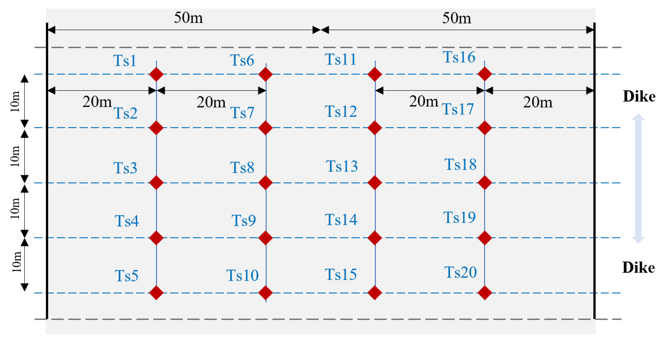
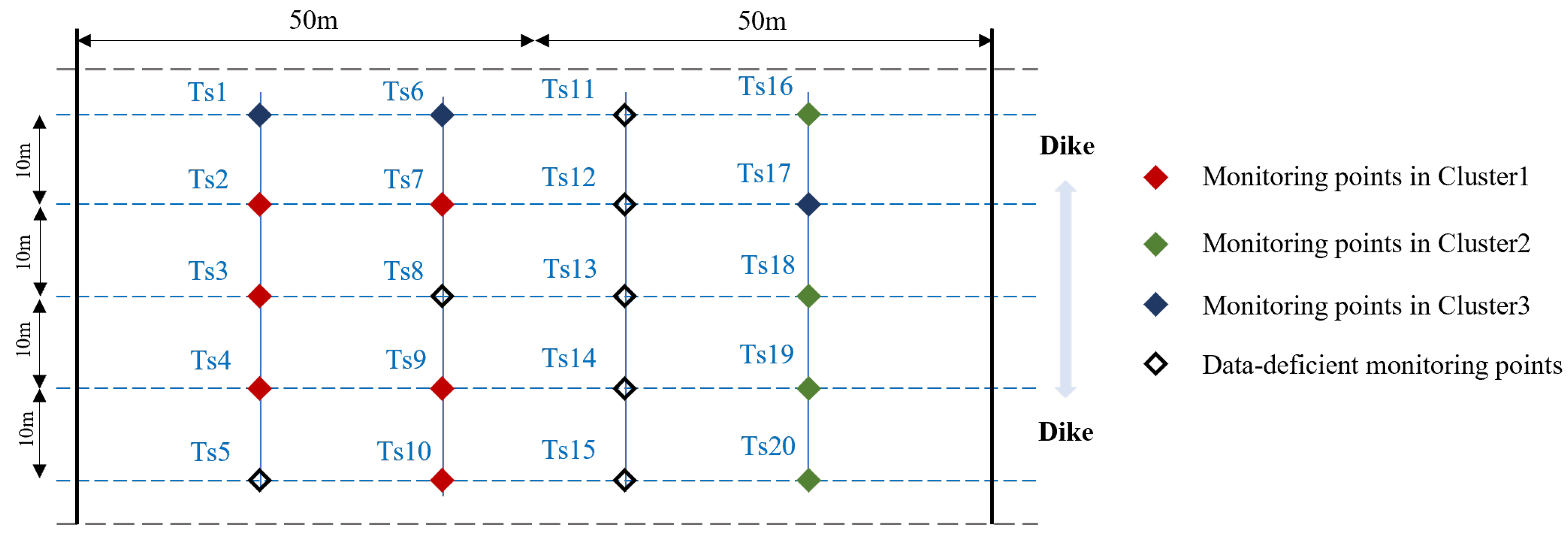
To provide an intuitive illustration of the monitoring layout, Figure 7 presents the spatial distribution of the seawall settlement monitoring points. The study area covers a region of 100 m × 40 m, where a total of 20 monitoring points (Ts1–Ts20) were deployed in a grid pattern, with a spacing of 20 m along the longitudinal direction of the dike and 10 m along the transverse direction. This arrangement was designed to comprehensively capture settlement characteristics across different regions, including both areas close to the dike and those farther away, thereby ensuring the spatial representativeness of the monitoring results. However, some points exhibited incomplete data records or significant measurement errors, which could potentially bias the modeling results if directly included. To ensure reliability and consistency, 13 monitoring points with relatively complete and high-quality records (Ts1–Ts7, Ts9, Ts10, and Ts16–Ts20) were selected as the research objects for subsequent analysis.
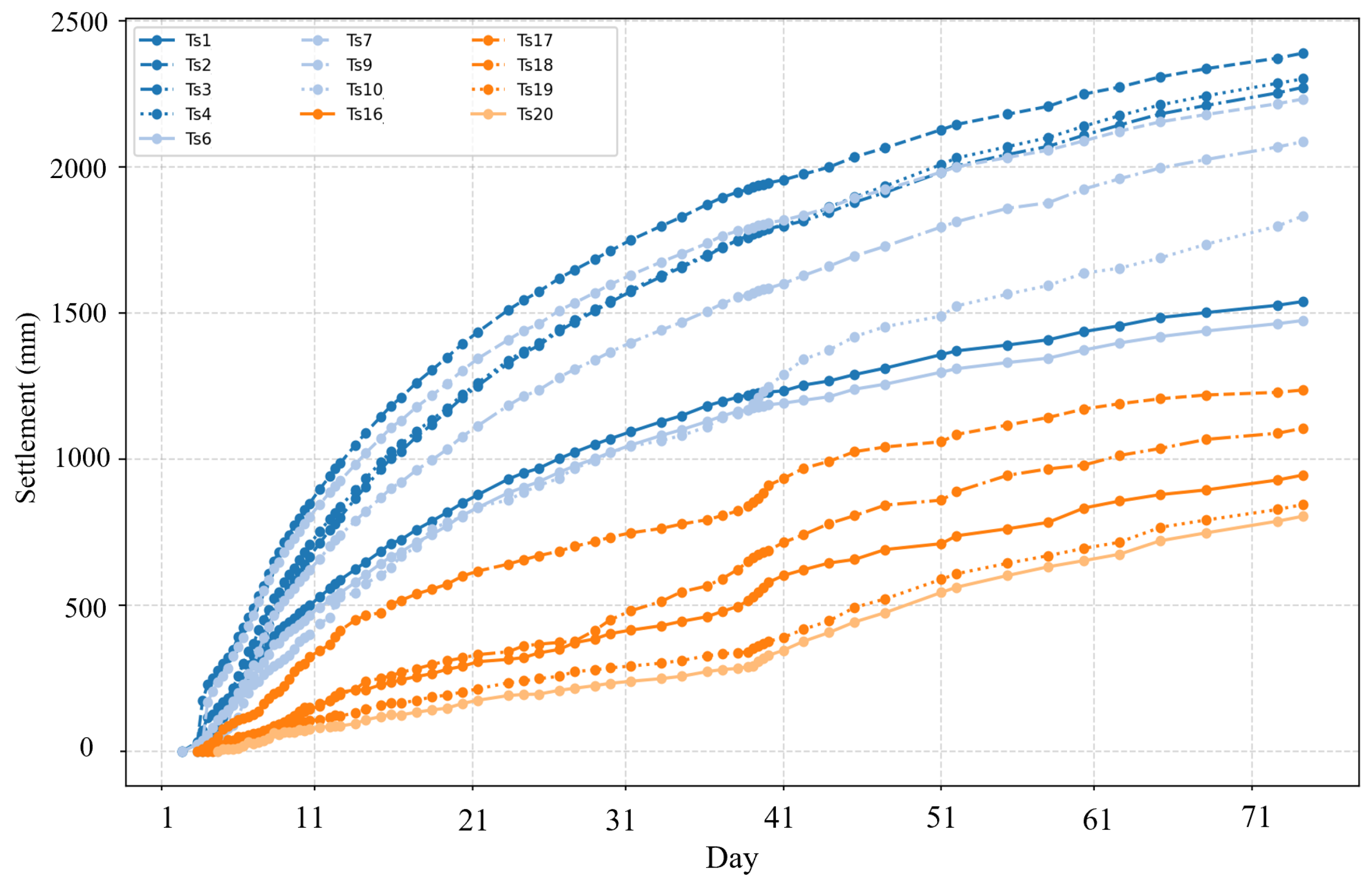
The temporal evolution of settlement data for these 13 monitoring points is illustrated in Figure 8. From the figure, it can be observed that all monitoring points exhibit a cumulative settlement growth over time, though the magnitudes and rates differ among locations. Some points, such as Ts2, Ts3, and Ts4, demonstrate larger settlement values exceeding 2000 mm, indicating areas of comparatively weaker soil stability. In contrast, points such as Ts16, Ts19, and Ts20 show relatively smaller settlement magnitudes, generally below 1000 mm, suggesting more stable foundation conditions. These variations highlight the spatial heterogeneity of seawall settlement and emphasize the necessity of adopting spatiotemporal models that can jointly capture both local and global deformation patterns. In addition, when modeling settlement behavior, relying solely on independent predictions at individual points makes it difficult to comprehensively capture the settlement patterns across different regions. By first clustering the monitoring points and then performing prediction within each cluster, the model can better identify similar settlement modes, thereby enhancing both prediction accuracy and robustness. This further highlights the necessity and effectiveness of a clustering–prediction integrated spatiotemporal panel strategy for multi-point settlement forecasting in seawall analysis.
Figure 9 presents the spatiotemporal evolution of cumulative settlement obtained via radial basis function (RBF) interpolation. The monitoring period spans 71 days, and seven snapshots are shown at 10-day intervals from day 10 to day 70 (the color scale indicates settlement). The maps reveal a sustained increase in settlement over time and pronounced spatial variability. Overall, the left-hand region exhibits larger and faster settlement, with denser isolines, indicating a higher settlement gradient; the central area shows a transitional pattern, while the right-hand region experiences smaller and more gradual changes. In addition, a localized high-value belt emerges in the upper part of the domain, reflecting location-dependent growth rates and marked spatiotemporal heterogeneity. These characteristics indicate differences in the temporal evolution patterns across monitoring points, further justifying time–series–based clustering.

4. Results

4.1. Clustering Results Based on DTW-HC Method

Figure 10 illustrates the pairwise distance matrix of the time series computed using Dynamic Time Warping (DTW). Each cell encodes the alignment-based dissimilarity between two series, with lighter colors indicating smaller distances (higher similarity) and darker colors indicating larger distances (lower similarity). We selected the number of clusters k using the elbow method applied to the within-cluster DTW dispersion. The curve shows a distinct elbow at k = 3, beyond which reductions in dispersion are marginal. Given the limited sample size (13 monitoring series), larger k would over-fragment the data and increase estimation variance in cluster-specific modeling. We therefore set k = 3 in the DTW–HC step. The heatmap reveals clear block structures of lower intra-cluster distances and higher inter-cluster distances, highlighting consistent similarity patterns among subsets of series. A distinct low-distance block is observed among Ts2, Ts3, Ts4, Ts7, Ts9, and Ts10, corresponding to Cluster 1; Ts16, Ts18, Ts19, and Ts20 form a compact low-distance area in the bottom-right corner, corresponding to Cluster 2; and Ts1, Ts6, and Ts17 also show strong mutual similarity, corresponding to Cluster 3. In contrast, inter-cluster regions are predominantly red, indicating substantial dissimilarities across clusters. This result demonstrates that DTW effectively captures shape-based similarities among time series and is highly consistent with the three-cluster partition obtained from the hierarchical clustering analysis.
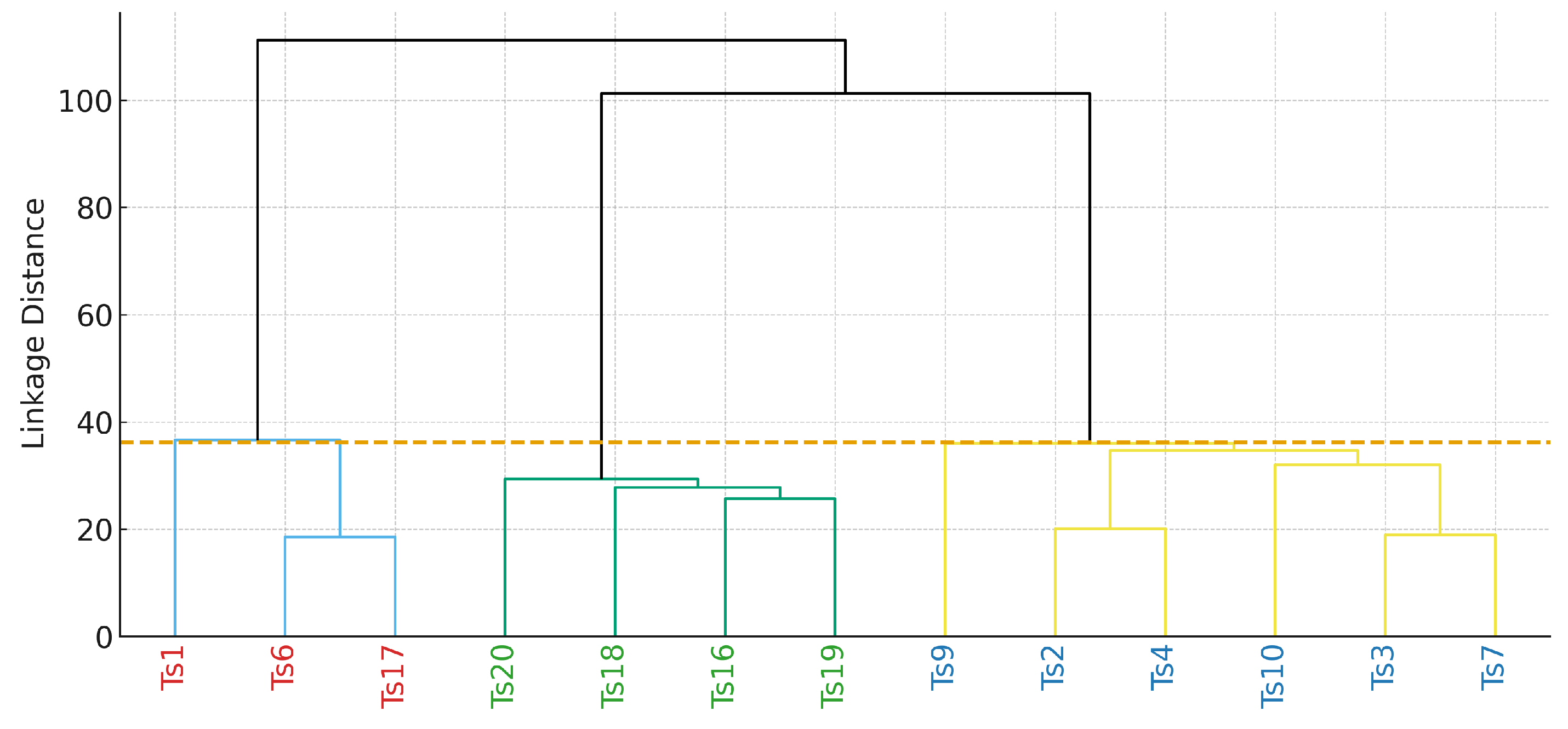
Figure 11 shows the dendrogram generated by applying Ward linkage hierarchical clustering to the DTW distance matrix. The x-axis denotes the time series indices, while the y-axis represents the linkage distance at each merging step. Leaf node labels are color-coded according to cluster membership (blue for Cluster 1, green for Cluster 2, and red for Cluster 3). A horizontal dashed line indicates the cut level used to obtain three clusters. The dendrogram clearly separates into three major branches, fully consistent with the final three-cluster solution, further validating the reliability of the clustering results.
Based on the spatiotemporal correlation analysis of settlement data, the monitoring points were divided into three distinct clusters, as shown in Figure 12. Specifically, Cluster 1 consists of Ts2, Ts3, Ts4, Ts7, Ts9, and Ts10, which are mainly distributed on the left side of the seawall. Cluster 2 includes Ts16, Ts18, Ts19, and Ts20, concentrated on the right side of the seawall and relatively close to the dike. Cluster 3 contains Ts1, Ts6, and Ts17, located in the central part of the seawall. The remaining monitoring points (Ts5, Ts8, Ts11, Ts12, Ts13, Ts14, Ts15) were excluded from the analysis due to incomplete or low-quality data. This clustering result reveals not only differences in settlement evolution patterns but also spatially structured distribution characteristics: monitoring points with similar settlement behaviors tend to be located in adjacent or functionally related regions of the seawall. Such spatially coherent clustering provides important insights into the underlying geotechnical and structural conditions of the seawall.
The temporal variation of settlement within each cluster is presented in Figure 13. As observed, monitoring points within the same cluster exhibit highly consistent settlement evolution patterns, while significant differences exist across clusters. Cluster 1 shows the largest settlement magnitude, exceeding 2000 mm by the end of the observation period, indicating relatively weak subsoil stability. Cluster 2 exhibits comparatively smaller settlement values (generally below 1000 mm), but its settlement curves fluctuate more strongly, suggesting that this region is more sensitive to external environmental influences. Cluster 3 demonstrates intermediate settlement levels (around 1200–1500 mm) and, similar to Cluster 1, shows smoother settlement curves with relatively stable growth trends. Overall, the settlement curves of Cluster 1 and Cluster 3 are smoother, whereas Cluster 2 is characterized by greater fluctuations. These findings not only reflect the spatial heterogeneity of seawall settlement but also confirm the rationality of the clustering approach. The results highlight that clustering effectively identifies distinct settlement patterns, thereby providing a solid foundation for subsequent multi-point prediction modeling.

4.2. Prediction Results Based on AJSO-LSTM Method

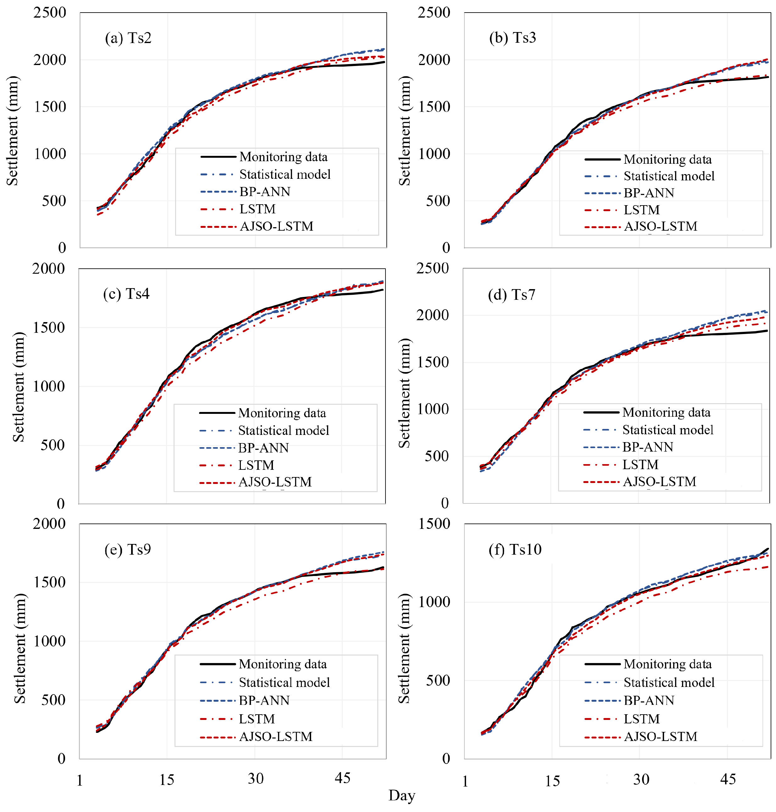
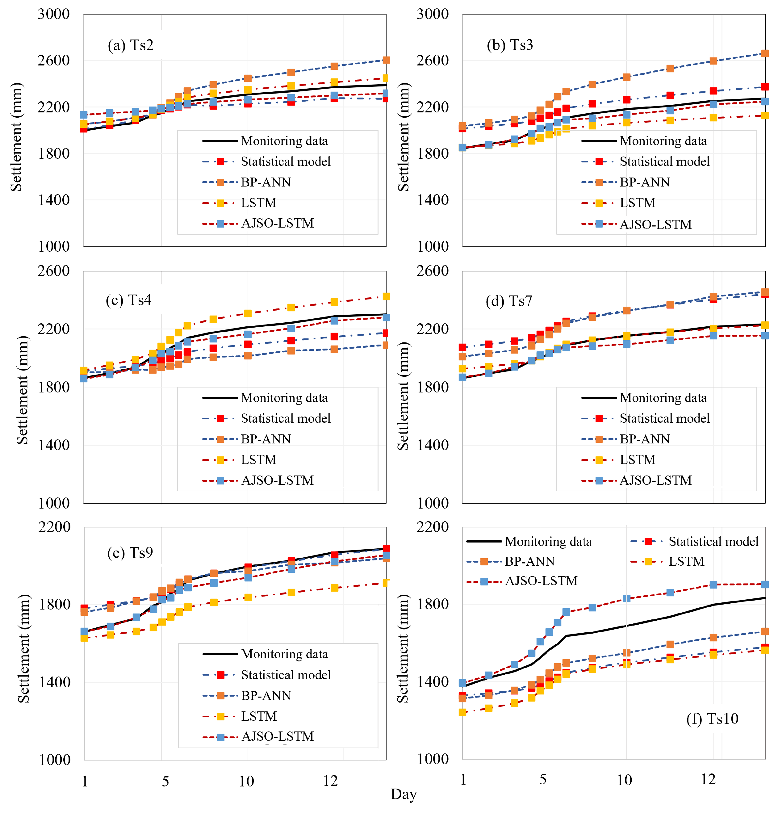
Figure 14 illustrates the comparison between monitored settlement data and the predictions generated by the proposed AJSO-LSTM model and three baseline methods, namely a statistical regression model, BP-ANN, and standard LSTM. The baselines were selected to cover both traditional approaches and widely used machine learning techniques: the statistical model represents conventional empirical analysis, BP-ANN is a representative shallow neural network for nonlinear fitting, and LSTM is a state-of-the-art recurrent neural network widely applied in time-series forecasting. The monitoring points included here belong to Cluster 1, which was identified using the DTW-HC clustering method (for details, see Section 4.1). We adopt chronological blocking throughout. Given a univariate time series at each monitoring point, samples are ordered in time and split as follows: the latest 20% of observations are held out as the test set (reported in Figure 15), while the earlier 80% are used for model development (results on the fitting portion are shown in Figure 14).
It can be seen from Figure 14 that the proposed AJSO-LSTM model achieves better overall agreement with the monitoring data compared with the baseline methods, exhibiting higher fitting accuracy across all points. The three baseline models also provide reasonably good predictions and are able to capture the general evolution trend of settlement, though some deviations are observed at certain stages. Overall, while the baseline models demonstrate satisfactory predictive capability, the proposed AJSO-LSTM outperforms them by more effectively capturing the nonlinear and temporal characteristics of the settlement process, thereby offering improved adaptability and accuracy. For brevity, only the time-evolution results for Cluster 1 are presented here, whereas the corresponding comparisons for Clusters 2 and 3 are provided in the Appendix A. For the perspective of computational complexity standard LSTM has forward complexity O B T ( H D + H 2 ) with the sequence length be T, batch size B, input dimension D, and hidden size H. Our AJSO-LSTM augments the LSTM core with a lightweight joint-sparsity/adaptive module that adds O ( B T H ) operations; this term is dominated by the H 2 main term, so AJSO-LSTM is asymptotically on par with LSTM and, in practice, exhibits similar training and inference time. A AJSO-LSTM with sliding-window inputs scales roughly linearly with T per window and is typically the lightest per step, but capturing long-range dependencies requires wider windows, increasing cost and error sensitivity. Statistical models are fastest on short sequences with very low per-step cost, yet their capacity to model strong nonlinearity and long-term dependencies is limited. Overall, AJSO-LSTM achieves a better accuracy–efficiency trade-off than these benchmarks, delivering improved robustness without a meaningful increase in computational load.
We reserve 20% of the dataset as the test set and perform 13-day ahead forecasts from the historical observations. Figure 15 reports predictions for Cluster 1, comparing the proposed AJSO-LSTM with three baselines (statistical model, BP-ANN, and LSTM). Despite minor pointwise deviations, the AJSO-LSTM exhibits the highest overall agreement with the monitoring data and the lowest prediction errors on the test set, while the baselines capture the general trend but are less accurate overall. The corresponding test results for Clusters 2 and 3 are provided in Appendix B.
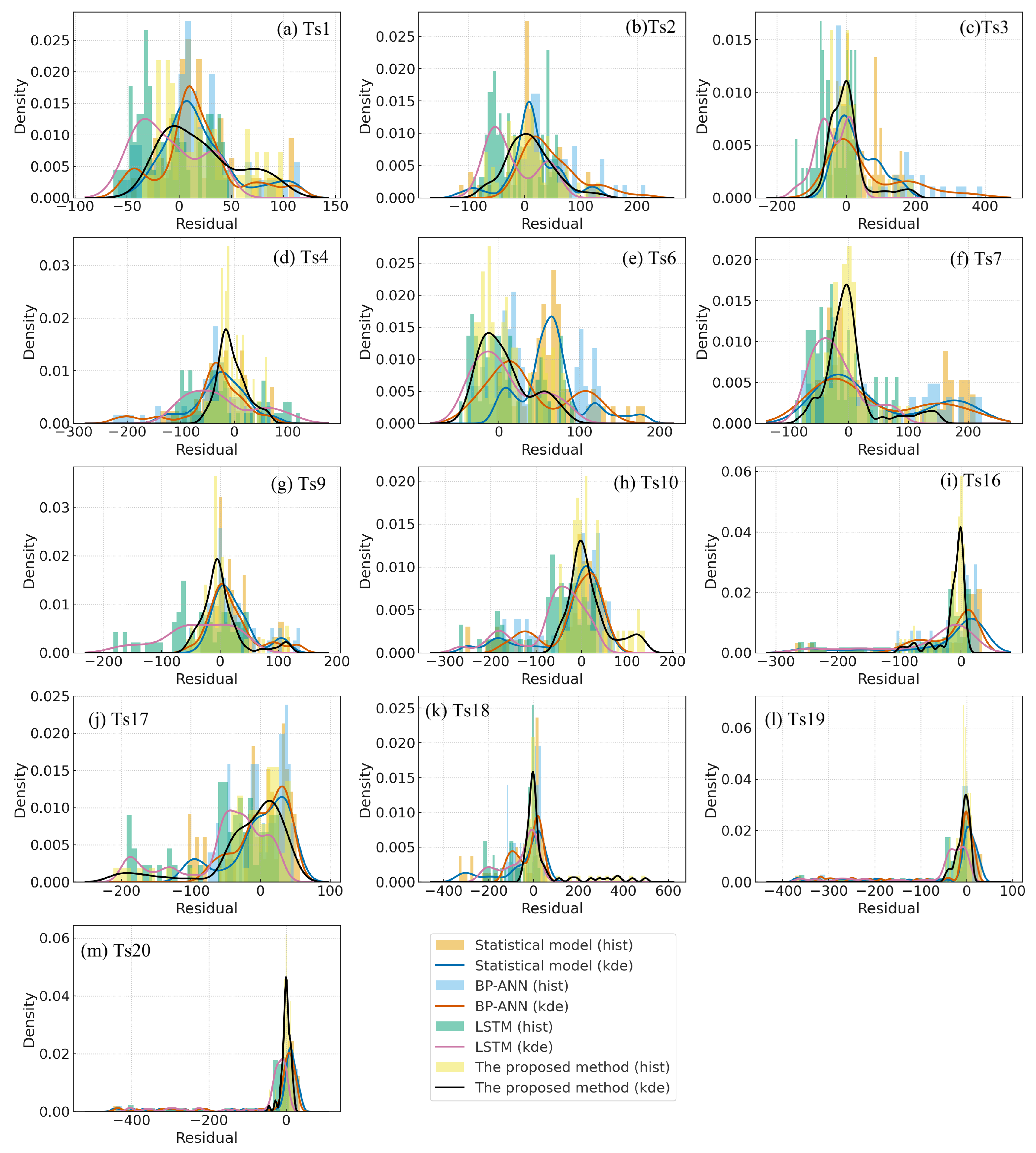
Figure 16 compares the residual probability density functions (via histograms) and their corresponding Kernel Density Estimation (KDE) curves for the proposed model and three baseline models across 13 monitoring points. The probability density characterizes the relative likelihood of residual magnitudes: the peak location indicates systematic bias, while the distribution width reflects dispersion. KDE is a non-parametric smoothing method that estimates a continuous density curve without assuming a specific distribution, providing insights into the shape, symmetry, and tail behavior of the residuals. Overall, many sites exhibit near-symmetric, unimodal residuals with modes close to zero, while others show multimodal distributions, suggesting more complex underlying behavior. Notably, residuals around zero are more densely concentrated, indicating that the majority of the data points are clustered near zero. Against this backdrop, the proposed model demonstrates superior error characteristics across nearly all sites: residuals are more concentrated, with higher modes, smaller variance, and lighter tails—indicating greater stability and reduced systematic bias. Although site-to-site differences remain, reflecting local conditions and data characteristics, these variations do not affect the overall conclusion that the proposed model is generally more robust.
Here, we selected the RMSE (Root Mean Squared Error) and MAPE (Mean Absolute Percentage Error) as the evaluation metrics to quantify the prediction precision of the proposed model and three baseline models. RMSE measures absolute deviation and is sensitive to large errors:
RMSE = 1 n t = 1 n y t y ^ t 2 .
MAPE measures relative error and is comparable across scales:
MAPE = 100 % n t = 1 n y t y ^ t y t .
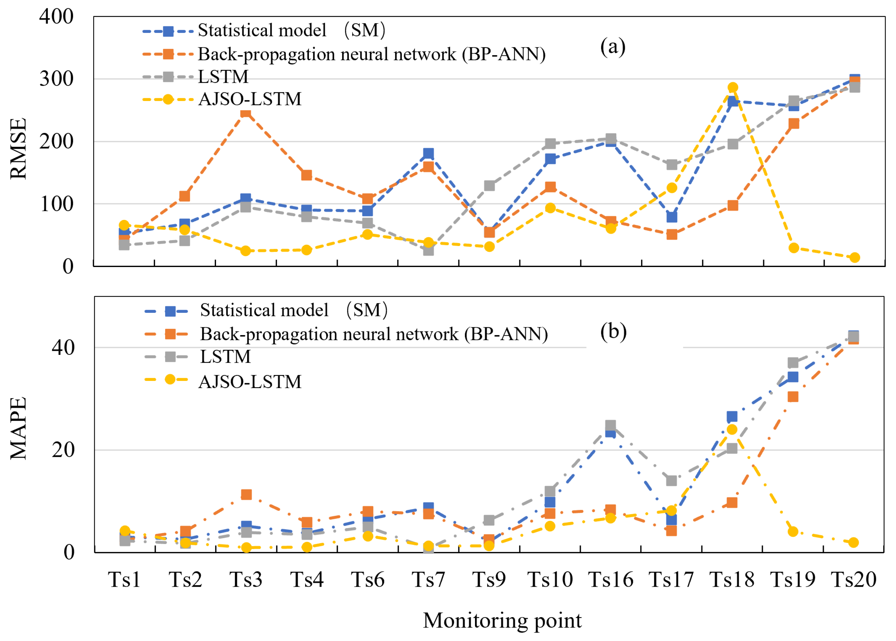
with n the number of time points, t { 1 , , n } the time index, y t observed value at time t, y ^ t — predicted value at time t. As y t = 0 occurs only at the initial time, we excluded the initial-time samples from the MAPE calculation to avoid undefined denominators. As indicated by Figure 17, in the test-set evaluation, the proposed AJSO-LSTM achieves the lowest RMSE and MAPE at the vast majority of monitoring points, outperforming all three baselines overall. Among the baselines, LSTM and BP-ANN generally perform better than the statistical model, as they more effectively capture nonlinear and temporal dependencies, whereas the statistical model reproduces only the gross trend and yields larger errors. Notably, all methods exhibit elevated errors at Ts18, and AJSO-LSTM also shows a relatively large deviation there—suggesting a data-quality issue or abrupt external forcing at that site rather than a lack of model robustness. Apart from Ts18, AJSO-LSTM maintains higher consistency and smaller deviations across sites, especially at Ts19 and Ts20, where competing models produce much larger errors while AJSO-LSTM remains accurate. Overall, the performance ranking is AJSO-LSTM (best), followed by LSTM and BP-ANN, and the statistical model trailing behind.

5. Discussions

The proposed framework, which integrates DTW-based hierarchical clustering (DTW-HC) with an AJSO-optimized LSTM model, demonstrates several important advantages for seawall settlement prediction. First, unlike conventional single-point or static-attribute-based clustering approaches, the use of DTW-HC enables the grouping of monitoring points according to their time series characteristics, thereby reflecting the temporal evolution patterns of settlement while simultaneously accounting for spatial heterogeneity. This significantly enhances the reliability of monitoring point classification and provides a more realistic representation of seawall behavior. Second, the introduction of the AJSO algorithm effectively addresses the limitations of conventional LSTM models, particularly their sensitivity to hyperparameter tuning and susceptibility to local optima. The optimization process improves model adaptability and robustness, leading to more accurate and stable predictions compared with statistical models, BP neural networks, and standard LSTM.
Comparative analysis on real engineering monitoring data confirms that the proposed framework outperforms traditional statistical models, BP-ANN, and conventional LSTM in terms of both classification validity and prediction accuracy. This highlights the effectiveness of combining time series–driven clustering with optimization-enhanced deep learning within a spatial panel data structure. DTW–HC improves consistency by clustering stations with similar responses; AJSO delivers the largest accuracy gain by stabilizing training and reducing overfitting; and spatial regularization enhances spatial smoothness and generalization. Overall, the full AJSO-LSTM yields the best performance, indicating that the three components are complementary.
Despite these achievements, several limitations remain. First, the proposed method requires sufficient monitoring data for both clustering and prediction, which may restrict its applicability to projects with limited or irregular datasets. Second, while DTW-HC provides an effective measure of time series similarity, its computational cost may increase with larger numbers of monitoring points and longer monitoring periods. Third, although AJSO improves the adaptability of LSTM, the model remains inherently data-driven, and its interpretability for engineering decision-making is limited compared with physics-based models.
Uncertainty and error propagation. In this study, uncertainty arises from two sources: (1) measurement-level uncertainty (aleatoric) and (2) modeling-level uncertainty (epistemic/modeling variability). First, measurement uncertainty stems from sensor resolution, environmental conditions, and operational factors. Although all stations use identical devices and consistent procedures—thereby reducing device-induced systematic bias—random noise, occasional outliers, and irregular sampling remain possible. Such variability can affect DTW-HC alignment and cluster composition and, in turn, propagate to per-cluster prediction errors. Consequently, station-wise differences that do not clearly exceed a reasonable measurement margin should be interpreted conservatively; for operational purposes, methods within this margin may be regarded as practically equivalent. Second, modeling-level uncertainty is inherent to intelligent algorithms and includes randomness from initialization, data splits, training order, optimizer stochasticity, and numerical/hardware non-determinism. In our cluster–then–predict pipeline, this variability may interact with clustering hyperparameters (e.g., DTW band width and the number of clusters), producing limited error propagation downstream. Given space and focus, we do not further quantify these effects; instead, we recommend interpreting small performance gaps within the combined bounds of measurement and modeling variability as functionally equivalent for maintenance decisions. Future work will provide a budget-aligned, formal uncertainty analysis with calibrated error bounds and hypothesis testing.
Future work can address these limitations in several ways. Hybrid frameworks that couple data-driven prediction with physical or mechanistic models may enhance both accuracy and interpretability. More efficient clustering algorithms or dimensionality-reduction techniques could be introduced to improve scalability for large-scale monitoring systems. Additionally, extending the spatial panel data framework to incorporate external environmental drivers (e.g., rainfall, tidal level, and soil properties) may further enhance its predictive capability. These directions could strengthen the generalizability of the proposed approach and expand its application to broader geotechnical and hydraulic engineering contexts.

6. Conclusions

This study proposed a novel framework for seawall settlement prediction by integrating Dynamic Time Warping-based Hierarchical Clustering (DTW-HC) with an Adaptive Joint Search Optimization enhanced Long Short-Term Memory (AJSO-LSTM) model. The main conclusions are as follows:
First, DTW-HC effectively groups monitoring points based on their temporal evolution, thereby constructing a spatial panel data structure that incorporates both spatial heterogeneity and time series characteristics. Compared with traditional static-attribute-based clustering, this approach provides a more realistic representation of seawall settlement behaviors. Second, by introducing AJSO to optimize the hyperparameters of LSTM, the proposed model successfully addresses common limitations, such as hyperparameter sensitivity, risk of local optima, and insufficient adaptability. This improvement significantly enhances both the robustness and generalization ability of the prediction model. Third, comparative experiments using seawall settlement monitoring data demonstrate that the proposed framework consistently outperforms three benchmark approaches, including conventional LSTM, statistical models, and BP neural networks (BP-ANN), in terms of prediction accuracy, robustness, and reliability.
In summary, the proposed DTW-HC and AJSO-LSTM framework offers an effective and practical tool for seawall settlement prediction, providing valuable support for seawall safety management and long-term service evaluation. Future research may further enhance the model by incorporating external environmental variables, improving interpretability, and scaling up computational efficiency for large-scale monitoring applications.

Author Contributions

Conceptualization, C.D.; methodology, X.L.; validation, Z.M. and Y.L.; formal analysis, C.D. and X.L.; data curation, C.D.; writing—original draft preparation, C.D.; writing—review and editing, X.L.; supervision, Z.M.; funding acquisition, Z.M. All authors have read and agreed to the published version of the manuscript.

Funding

This research was funded by Zhejiang Provincial Natural Science Foundation of China (Grant No. LZJWY24E090005), and Huzhou Science and Technology Plan Project (Grant No. 2024G263).

Data Availability Statement

Data available upon request.

Conflicts of Interest

The authors declare no conflicts of interest.

Abbreviations

The following abbreviations are used in this manuscript:
AJSOAdaptive Joint Search Optimization
LSTMLong Short-Term Memory
DTWDynamic Time Warping
HCHierarchical Clustering
BP-ANNBackpropagation Artificial Neural Network
RBFRadial Basis Function
RMSERoot Mean Squared Error
MAPEMean Absolute Percentage Error
KDEKernel Density Estimation
MIMOMulti-Input Multi-Output

Appendix A. Fitting Settlements of Cluster 2 and Cluster 3 Points
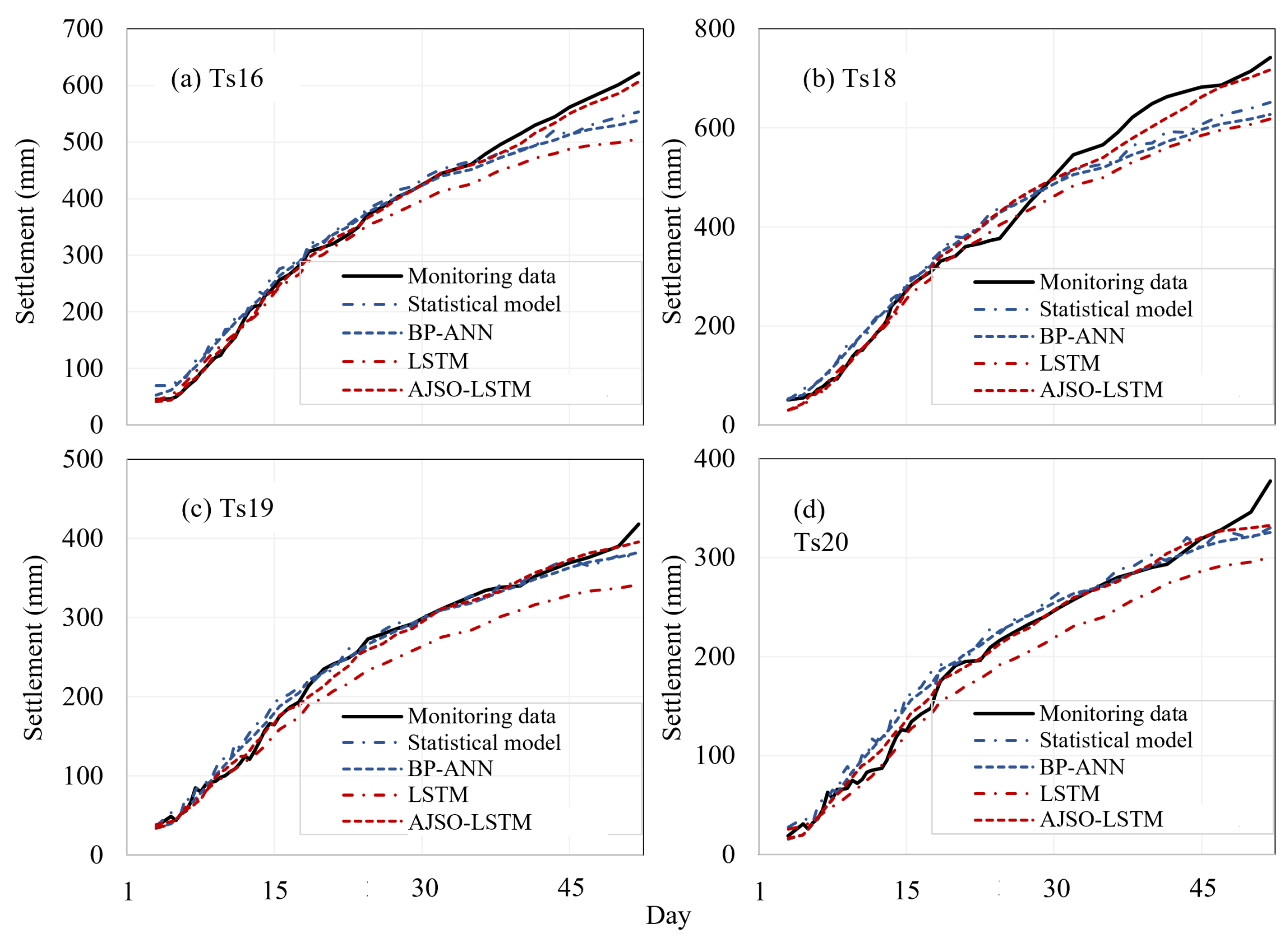
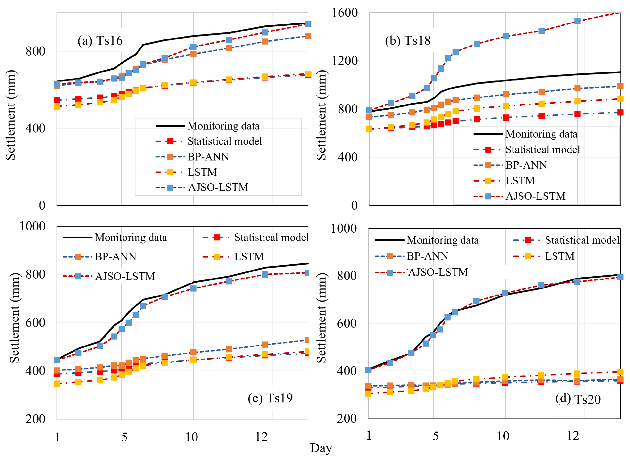
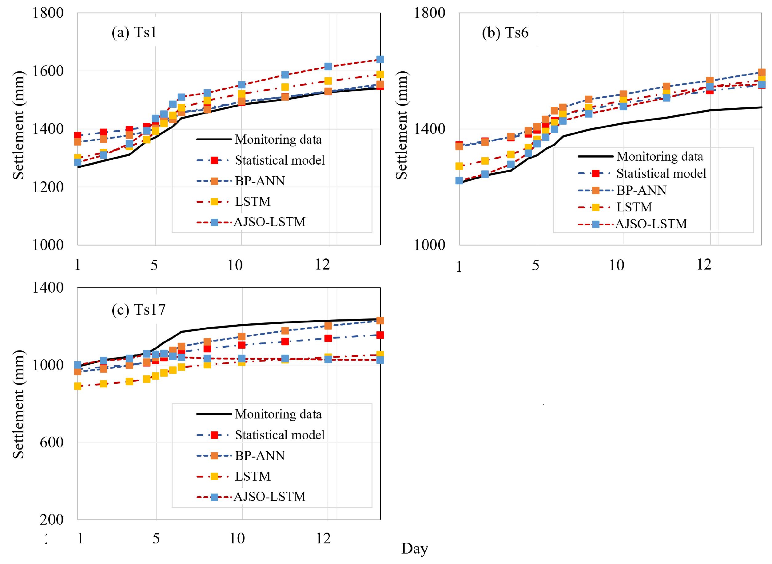
Figure A1 and Figure A2 illustrate the time evolution of monitored and predicted settlements at cluster 2 and cluster 3, respectively.
Figure A1. Time evolution of monitored and predicted settlements (fitting data) at cluster 2 points using the proposed model and baseline methods: (a) Ts16, (b) Ts18, (c) Ts19, (d) Ts20.
Jmse 13 02053 g0a1
Figure A2. Time evolution of monitored and predicted settlements (fitting data) at cluster 3 points using the proposed model and baseline methods: (a) Ts1, (b) Ts6, (c) Ts17.
Jmse 13 02053 g0a2

Appendix B. Testing Settlements of Cluster 2 and Cluster 3 Points

Figure A3 reports test-set predictions for Cluster 2 over a 13-day horizon. Overall, the AJSO-LSTM aligns most closely with the monitoring data, yielding smaller deviations and more stable errors across time. The three baselines (statistical model, BP-ANN, and LSTM) capture the general settlement trend but exhibit local discrepancies (e.g., response lags or amplitude biases). These results indicate that AJSO-LSTM provides superior generalization performance for Cluster 2.
Figure A3. Monitored and predicted settlements (testing data) at cluster 2 points using the proposed model and baseline methods: (a) Ts16, (b) Ts18, (c) Ts19, (d) Ts20.
Jmse 13 02053 g0a3
Figure A4 presents the 13-day test-set forecasts for Cluster 3. Similar to Cluster 2, the AJSO-LSTM shows the highest agreement with observations and lower prediction errors across most timestamps, whereas the baselines track the overall trend but under- or over-estimate during change points or abrupt stages. The findings further confirm the robustness and accuracy advantages of AJSO-LSTM across different clusters.
Figure A4. Monitored and predicted settlements (testing data) at cluster 3 points using the proposed model and baseline methods: (a) Ts1, (b) Ts6, (c) Ts17.
Jmse 13 02053 g0a4

References

  1. Mi, C.; Gao, J.; Song, Z.; Liu, Y. Hydrodynamic wave forces on two side-by-side barges subjected to nonlinear focused wave groups. Ocean Eng. 2025, 317, 120056. [Google Scholar] [CrossRef]
  2. Koraim, A.; Heikal, E.; Zaid, A.A. Hydrodynamic characteristics of porous seawall protected by submerged breakwater. Appl. Ocean Res. 2014, 46, 1–14. [Google Scholar] [CrossRef]
  3. Gong, S.; Gao, J.; Yan, M.; Song, Z.; Shi, H. Effects of floater motion on wave loads during steady-state gap resonance occurring between two non-identical boxes. Ocean Eng. 2025, 323, 120649. [Google Scholar] [CrossRef]
  4. Galili, E.; Benjamin, J.; Eshed, V.; Rosen, B.; McCarthy, J.; Horwitz, L.K. A submerged 7000-year-old village and seawall demonstrate earliest known coastal defence against sea-level rise. PLoS ONE 2019, 14, e0222560. [Google Scholar] [CrossRef] [PubMed]
  5. Hazarika, H.; Fukumoto, Y. Sustainable solution for seawall protection against tsunami-induced damage. Int. J. Geomech. 2016, 16, C4016005. [Google Scholar] [CrossRef]
  6. Li, J.; Meng, Z.; Zhang, J.; Chen, Y.; Yao, J.; Li, X.; Qin, P.; Liu, X.; Cheng, C. Prediction of seawater intrusion run-up distance based on K-means clustering and ANN model. J. Mar. Sci. Eng. 2025, 13, 377. [Google Scholar] [CrossRef]
  7. Hosseinzadeh, N.; Ghiasian, M.; Andiroglu, E.; Lamere, J.; Rhode-Barbarigos, L.; Sobczak, J.; Sealey, K.S.; Suraneni, P. Concrete seawalls: A review of load considerations, ecological performance, durability, and recent innovations. Ecol. Eng. 2022, 178, 106573. [Google Scholar] [CrossRef]
  8. Kraus, N.C. The effects of seawalls on the beach: An extended literature review. J. Coast. Res. 1988, SI 4, 1–28. [Google Scholar]
  9. Zehro, K. Specifications and types of seawall structures needed to protect beaches from sand erosion and storm disasters. Int. J. Adv. Eng. Sci. Appl. 2021, 2, 13–18. [Google Scholar] [CrossRef]
  10. Hu, Y.; Gu, C.; Meng, Z.; Shao, C. Improve the model stability of Dam’s displacement prediction using a numerical-statistical combined model. Ieee Access 2020, 8, 147482–147493. [Google Scholar] [CrossRef]
  11. Salazar, F.; Toledo, M.; Oñate, E.; Morán, R. An empirical comparison of machine learning techniques for dam behaviour modelling. Struct. Saf. 2015, 56, 9–17. [Google Scholar] [CrossRef]
  12. Gao, J.; Hou, L.; Liu, Y.; Shi, H. Influences of bragg reflection on harbor resonance triggered by irregular wave groups. Ocean Eng. 2024, 305, 117941. [Google Scholar] [CrossRef]
  13. Gao, J.; Ma, X.; Dong, G.; Chen, H.; Liu, Q.; Zang, J. Investigation on the effects of Bragg reflection on harbor oscillations. Coast. Eng. 2021, 170, 103977. [Google Scholar] [CrossRef]
  14. Goel, S.; Imielinski, T. Prediction-based monitoring in sensor networks: Taking lessons from MPEG. ACM SIGCOMM Comput. Commun. Rev. 2001, 31, 82–98. [Google Scholar] [CrossRef]
  15. Yao, K.; Wen, Z.; Yang, L.; Chen, J.; Hou, H.; Su, H. A multipoint prediction model for nonlinear displacement of concrete dam. Comput. Aided Civ. Infrastruct. Eng. 2022, 37, 1932–1952. [Google Scholar] [CrossRef]
  16. Tatin, M.; Briffaut, M.; Dufour, F.; Simon, A.; Fabre, J.P. Statistical modelling of thermal displacements for concrete dams: Influence of water temperature profile and dam thickness profile. Eng. Struct. 2018, 165, 63–75. [Google Scholar] [CrossRef]
  17. Goda, K. Statistical modeling of joint probability distribution using copula: Application to peak and permanent displacement seismic demands. Struct. Saf. 2010, 32, 112–123. [Google Scholar] [CrossRef]
  18. Xi, G.y.; Yue, J.p.; Zhou, B.x.; Tang, P. Application of an artificial immune algorithm on a statistical model of dam displacement. Comput. Math. Appl. 2011, 62, 3980–3986. [Google Scholar] [CrossRef]
  19. Liu, X.; Jiang, S.H.; Xie, J.; Li, X. Bayesian inverse analysis with field observation for slope failure mechanism and reliability assessment under rainfall accounting for nonstationary characteristics of soil properties. Soils Found. 2025, 65, 101568. [Google Scholar] [CrossRef]
  20. Chen, H.; Huang, S.; Qiu, H.; Xu, Y.P.; Teegavarapu, R.S.; Guo, Y.; Nie, H.; Xie, H.; Xie, J.; Shao, Y.; et al. Assessment of ecological flow in river basins at a global scale: Insights on baseflow dynamics and hydrological health. Ecol. Indic. 2025, 178, 113868. [Google Scholar] [CrossRef]
  21. Zhou, J.; Fu, K.; Liang, S.; Li, J.; Liang, J.; An, X.; Liu, Y. Extracting Water Surfaces of the Dike-Pond System from High Spatial Resolution Images Using Deep Learning Methods. Remote Sens. 2024, 17, 111. [Google Scholar] [CrossRef]
  22. Qin, P.; Cheng, C. Prediction of Seawall Settlement Based on a Combined LS-ARIMA Model. Math. Probl. Eng. 2017, 2017, 7840569. [Google Scholar] [CrossRef]
  23. Meng, Z.; Hu, Y.; Jiang, S.; Zheng, S.; Zhang, J.; Yuan, Z.; Yao, S. Slope Deformation Prediction Combining Particle Swarm Optimization-Based Fractional-Order Grey Model and K-Means Clustering. Fractal Fract. 2025, 9, 210. [Google Scholar] [CrossRef]
  24. Frangopol, D.M.; Strauss, A.; Kim, S. Use of monitoring extreme data for the performance prediction of structures: General approach. Eng. Struct. 2008, 30, 3644–3653. [Google Scholar] [CrossRef]
  25. Liu, X.; Li, X.; Ma, G.; Rezania, M. Characterization of spatially varying soil properties using an innovative constraint seed method. Comput. Geotech. 2025, 183, 107184. [Google Scholar] [CrossRef]
  26. Mata, J.; Salazar, F.; Barateiro, J.; Antunes, A. Validation of machine learning models for structural dam behaviour interpretation and prediction. Water 2021, 13, 2717. [Google Scholar] [CrossRef]
  27. Li, M.; Li, M.; Ren, Q.; Li, H.; Song, L. DRLSTM: A dual-stage deep learning approach driven by raw monitoring data for dam displacement prediction. Adv. Eng. Informatics 2022, 51, 101510. [Google Scholar] [CrossRef]
  28. Zhang, J.; Zhang, X.; Li, H.; Fan, Y.; Meng, Z.; Liu, D.; Pan, S. Optimization of Water Quantity Allocation in Multi-Source Urban Water Supply Systems Using Graph Theory. Water 2024, 17, 61. [Google Scholar] [CrossRef]
  29. Chen, H.; Xu, B.; Qiu, H.; Huang, S.; Teegavarapu, R.S.; Xu, Y.P.; Guo, Y.; Nie, H.; Xie, H. Adaptive assessment of reservoir scheduling to hydrometeorological comprehensive dry and wet condition evolution in a multi-reservoir region of southeastern China. J. Hydrol. 2025, 648, 132392. [Google Scholar] [CrossRef]
  30. Mugnaini, V.; Fragonara, L.Z.; Civera, M. A machine learning approach for automatic operational modal analysis. Mech. Syst. Signal Process. 2022, 170, 108813. [Google Scholar] [CrossRef]
  31. Liu, Y.; Zhang, L.; Xin, J.; Peng, S. TPS-GNN: Predictive model for bridge health monitoring data based on temporal periodicity and global spatial distribution characteristics. Struct. Health Monit. 2025, 14759217251330971. [Google Scholar] [CrossRef]
  32. Li, Z.H.; Cui, J.X.; Lu, H.P.; Zhou, F.; Diao, Y.L.; Li, Z.X. Prediction model of measurement errors in current transformers based on deep learning. Rev. Sci. Instruments 2024, 95, 044704. [Google Scholar] [CrossRef] [PubMed]
  33. Bi, J.; Li, J.; Wu, K.; Chen, Z.; Chen, S.; Jiang, L.; Feng, D.; Deng, P. A physics-informed spatial-temporal neural network for reservoir simulation and uncertainty quantification. SPE J. 2024, 29, 2026–2043. [Google Scholar] [CrossRef]
  34. Qu, X.; Yang, J.; Chang, M. A Deep Learning Model for Concrete Dam Deformation Prediction Based on RS-LSTM. J. Sensors 2019, 2019, 4581672. [Google Scholar] [CrossRef]
  35. Li, Y.; Bao, T.; Gong, J.; Shu, X.; Zhang, K. The prediction of dam displacement time series using STL, extra-trees, and stacked LSTM neural network. IEEE Access 2020, 8, 94440–94452. [Google Scholar] [CrossRef]
  36. Madiniyeti, J.; Chao, Y.; Li, T.; Qi, H.; Wang, F. Concrete dam deformation prediction model research based on SSA–LSTM. Appl. Sci. 2023, 13, 7375. [Google Scholar] [CrossRef]
  37. Zheng, S.; Gu, C.; Shao, C.; Hu, Y.; Xu, Y.; Huang, X. A novel prediction model for seawall deformation based on CPSO-WNN-LSTM. Mathematics 2023, 11, 3752. [Google Scholar] [CrossRef]
  38. Qin, P.; Cheng, C.; Meng, Z.; Ding, C.; Zheng, S.; Su, H. Multi-Point Seawall Settlement Prediction with Limited Data Volume Using an Improved Fractional-Order Grey Model. Fractal Fract. 2024, 8, 423. [Google Scholar] [CrossRef]
  39. Li, X.; Liu, X.; Li, C.Z.; Hu, Z.; Shen, G.Q.; Huang, Z. Foundation pit displacement monitoring and prediction using least squares support vector machines based on multi-point measurement. Struct. Health Monit. 2019, 18, 715–724. [Google Scholar] [CrossRef]
  40. Li, Y.; Min, K.; Zhang, Y.; Wen, L. Prediction of the failure point settlement in rockfill dams based on spatial-temporal data and multiple-monitoring-point models. Eng. Struct. 2021, 243, 112658. [Google Scholar] [CrossRef]
  41. Fattahi, H.; Bayatzadehfard, Z. Forecasting surface settlement caused by shield tunneling using ANN-BBO model and ANFIS based on clustering methods. J. Eng. Geol. 2018, 12, 55–84. [Google Scholar]
  42. Beiranvand, B.; Rajaee, T.; Komasi, M. Presenting the AI models in predicting the settlement of earth dams using the results of spatiotemporal clustering and k-means algorithm. Sci. Rep. 2024, 14, 10207. [Google Scholar] [CrossRef] [PubMed]
  43. Aghabozorgi, S.; Shirkhorshidi, A.S.; Wah, T.Y. Time-series clustering–a decade review. Inf. Syst. 2015, 53, 16–38. [Google Scholar] [CrossRef]
  44. Liao, T.W. Clustering of time series data—A survey. Pattern Recognit. 2005, 38, 1857–1874. [Google Scholar] [CrossRef]
  45. Rani, S.; Sikka, G. Recent techniques of clustering of time series data: A survey. Int. J. Comput. Appl. 2012, 52, 15. [Google Scholar] [CrossRef]
  46. Sammour, M.; Othman, Z.A.; Rus, A.M.M.; Mohamed, R. Modified dynamic time warping for hierarchical clustering. Int. J. Adv. Sci. Eng. Inf. Technol. 2019, 9, 1481–1487. [Google Scholar] [CrossRef]
  47. Petitjean, F.; Ketterlin, A.; Gançarski, P. A global averaging method for dynamic time warping, with applications to clustering. Pattern Recognit. 2011, 44, 678–693. [Google Scholar] [CrossRef]
  48. Li, H. Time works well: Dynamic time warping based on time weighting for time series data mining. Inf. Sci. 2021, 547, 592–608. [Google Scholar] [CrossRef]
  49. Zhao, Z.; Li, D.; Xu, X.; Zhang, D. An adaptive joint operating parameters optimization approach for active direct methanol fuel cells. Energies 2023, 16, 2167. [Google Scholar] [CrossRef]
  50. Zhang, J.; Wan, Z.; Liao, J. Adaptive joint optimization for 3D reconstruction with differentiable rendering. IEEE Trans. Vis. Comput. Graph. 2022, 29, 3039–3051. [Google Scholar] [CrossRef]
  51. Sherstinsky, A. Fundamentals of recurrent neural network (RNN) and long short-term memory (LSTM) network. Phys. D Nonlinear Phenom. 2020, 404, 132306. [Google Scholar] [CrossRef]
  52. Yu, Y.; Si, X.; Hu, C.; Zhang, J. A review of recurrent neural networks: LSTM cells and network architectures. Neural Comput. 2019, 31, 1235–1270. [Google Scholar] [CrossRef]
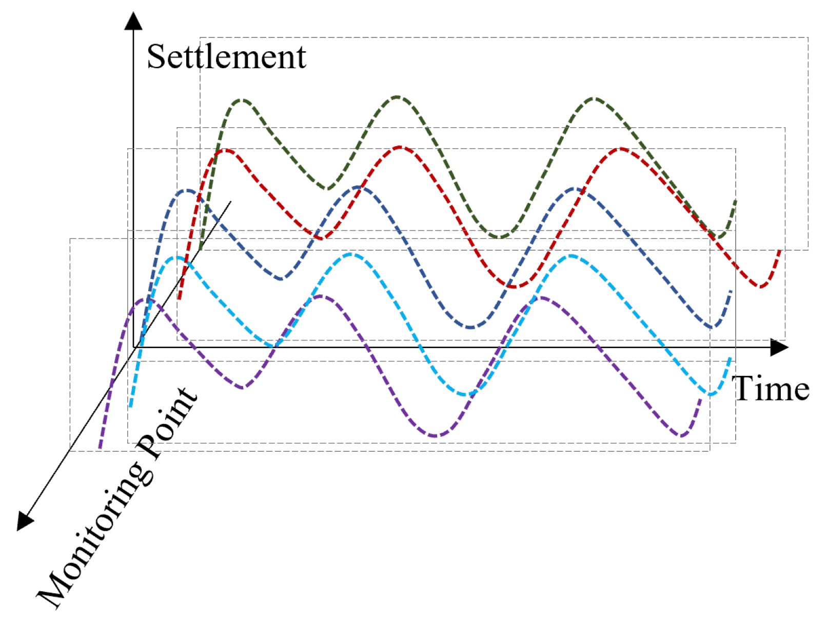
Figure 1. The structure of several time series data.
Jmse 13 02053 g001
Figure 2. The evolution of data structures in monitoring data prediction.
Jmse 13 02053 g002
Figure 3. The flow chart of LSTM method.
Jmse 13 02053 g003
Figure 4. The flow chart of AJSO-LSTM method.
Jmse 13 02053 g004
Figure 5. The flow chart of the DTW-HC clustering method.
Jmse 13 02053 g005
Figure 6. All monitoring instruments installed within the test section of the seawall: (a) plan layout, (b) longitudinal layout.
Jmse 13 02053 g006
Figure 7. Spatial distribution of seawall settlement monitoring points.
Jmse 13 02053 g007
Figure 8. Time variation of the settlement data for the 13 selected monitoring points.
Jmse 13 02053 g008
Figure 9. Time variation of interpolated settlement of the selected engineering case at (a) 10 days, (b) 20 days, (c) 30 days, (d) 40 days, (e) 50 days, (f) 60 days, and (g) 70 days since the first record day.
Jmse 13 02053 g009
Figure 10. DTW distance matrix heatmap.
Jmse 13 02053 g010
Figure 11. Hierarchical clustering dendrogram.
Jmse 13 02053 g011
Figure 12. Spatial distribution of the three clusters.
Jmse 13 02053 g012
Figure 13. The settlement data of three clusters (a) cluster 1, (b) cluster 2, (c) cluster 3.
Jmse 13 02053 g013
Figure 14. Time evolution of monitored and predicted settlements (fitting data) at cluster 1 points using the proposed model and baseline methods: (a) Ts2, (b) Ts3, (c) Ts4, (d) Ts7, (e) Ts9, and (f) Ts10.
Jmse 13 02053 g014
Figure 15. Monitored and predicted settlements (testing data) at cluster 1 points using the proposed model and baseline methods: (a) Ts2, (b) Ts3, (c) Ts4, (d) Ts7, (e) Ts9, and (f) Ts10.
Jmse 13 02053 g015
Figure 16. The probability density distribution of residual of the proposed model and three baseline models for all monitoring points: (a) Ts1, (b) Ts2, (c) Ts3, (d) Ts4, (e) Ts6, (f) Ts7, (g) Ts9, (h) Ts10, (i) Ts16, (j) Ts17, (k) Ts18, (l) Ts19, and (m) Ts20.
Jmse 13 02053 g016
Figure 17. Comparison of the evaluation metrics (a) RMSE and (b) MAPE between the proposed model and baseline models.
Jmse 13 02053 g017
Table 1. Panel data structure.
Points123t
1 δ 11 δ 12 δ 13 δ 1 t
2 δ 21 δ 22 δ 23 δ 2 t
3 δ 31 δ 32 δ 33 δ 3 t
n δ n 1 δ n 2 δ n 3 δ n t
Table 2. Spatial panel data structure.
Points123t
1 δ 1 ( x 1 , y 1 , t 1 ) δ 2 ( x 1 , y 1 , t 1 ) δ 3 ( x 1 , y 1 , t 1 ) δ t ( x 1 , y 1 , t 1 )
2 δ 1 ( x 2 , y 2 , t 2 ) δ 2 ( x 2 , y 2 , t 2 ) δ 3 ( x 2 , y 2 , t 2 ) δ t ( x 2 , y 2 , t 2 )
3 δ 1 ( x 3 , y 3 , t 3 ) δ 2 ( x 3 , y 3 , t 3 ) δ 3 ( x 3 , y 3 , t 3 ) δ t ( x 3 , y 3 , t 3 )
n δ 1 ( x n , y n , t n ) δ 2 ( x n , y n , t n ) δ 3 ( x n , y n , t n ) δ t ( x n , y n , t n )
Table 3. Final AJSO-selected configurations per cluster.
ClusterLHiddenBatchLR λ s r (m)h (m)w γ sDTW
C115164 1.0 × 10 3 1.0 × 10 3 251560.05
C210124 1.0 × 10 3 1.0 × 10 4 251260.02
C312164 1.0 × 10 3 1.0 × 10 3 251560.05
Disclaimer/Publisher’s Note: The statements, opinions and data contained in all publications are solely those of the individual author(s) and contributor(s) and not of MDPI and/or the editor(s). MDPI and/or the editor(s) disclaim responsibility for any injury to people or property resulting from any ideas, methods, instructions or products referred to in the content.