Article

Attentive Neural Processes for Few-Shot Learning Anomaly-Based Vessel Localization Using Magnetic Sensor Data

by
Luis Fernando Fernández-Salvador
*,†,
Borja Vilallonga Tejela
,
Alejandro Almodóvar
,
Juan Parras
* and
Santiago Zazo
Information Processing and Telecommunications Center, ETSI Telecomunicación, Universidad Politécnica de Madrid (UPM), Avda. Complutense, 30, 28040 Madrid, Spain
*
Authors to whom correspondence should be addressed.
These authors contributed equally to this work.
J. Mar. Sci. Eng. 2025, 13(9), 1627; https://doi.org/10.3390/jmse13091627
Submission received: 24 July 2025 / Revised: 18 August 2025 / Accepted: 20 August 2025 / Published: 26 August 2025
(This article belongs to the Section Ocean Engineering)

Abstract

Underwater vessel localization using passive magnetic anomaly sensing is a challenging problem due to the variability in vessel magnetic signatures and operational conditions. Data-based approaches may fail to generalize even to slightly different conditions. Thus, we propose an Attentive Neural Process (ANP) approach, in order to take advantage of its few-shot capabilities to generalize, for robust localization of underwater vessels based on magnetic anomaly measurements. Our ANP models the mapping from multi-sensor magnetic readings to position as a stochastic function: it cross-attends to a variable-size set of context points and fuses these with a global latent code that captures trajectory-level factors. The decoder outputs a Gaussian over coordinates, providing both point estimates and well-calibrated predictive variance. We validate our approach using a comprehensive dataset of magnetic disturbance fields, covering 64 distinct vessel configurations (combinations of varying hull sizes, submersion depths (water-column height over a seabed array), and total numbers of available sensors). Six magnetometer sensors in a fixed circular arrangement record the magnetic field perturbations as a vessel traverses sinusoidal trajectories. We compare the ANP against baseline multilayer perceptron (MLP) models: (1) base MLPs trained separately on each vessel configuration, and (2) a domain-randomized search (DRS) MLP trained on the aggregate of all configurations to evaluate generalization across domains. The results demonstrate that the ANP achieves superior generalization to new vessel conditions, matching the accuracy of configuration-specific MLPs while providing well-calibrated uncertainty quantification. This uncertainty-aware prediction capability is crucial for real-world deployments, as it can inform adaptive sensing and decision-making. Across various in-distribution scenarios, the ANP halves the mean absolute error versus a domain-randomized MLP (0.43 m vs. 0.84 m). The model is even able to generalize to out-of-distribution data, which means that our approach has the potential to facilitate transferability from offline training to real-world conditions.

1. Introduction

Accurate localization of marine vessels (such as ships, submarines, or autonomous underwater vehicles) is critical for navigation and tracking in marine environments. Acoustic long-baseline (LBL) and short-baseline (SBL) systems achieve metre-level accuracy, but their beacons are expensive to deploy and suffer from multipath and Doppler distortion at long range [1]. Global Navigation Satellite System (GNSS) fixes require surfacing, which is often unacceptable for stealth assets. By contrast, passive magnetic-anomaly sensing is attractive because tri-axial magnetometers are inexpensive, silent, and the geomagnetic field penetrates seawater with negligible attenuation [2]. Recent data-driven frameworks have even matched acoustic baselines using only magnetic cues [3]. In this study, we focus on addressing off-board magnetic localization/tracking using a fixed seabed sensor array; throughout, “depth” denotes the water-column height between the vessel and the sensor plane (see Section 3).
Despite these advances, purely magnetic localization remains brittle. The induced field depends non-linearly on hull geometry, orientation, and depth; sensor dropouts are common in cluttered bays; and real trajectories rarely match the limited configurations seen in training. Domain randomization (DR) mitigates the sim-to-real gap by perturbing simulator parameters, yet deterministic models still extrapolate poorly and provide no measure of confidence [4,5]. Safety-critical navigation, however, demands calibrated uncertainty so planners can reason about risk.
Even so, fixed neural networks still struggle to generalize to unseen conditions and cannot quantify their own confidence. This motivates meta-learning approaches that adapt from limited data. Neural Processes (NPs) learn a distribution over functions and can rapidly adapt by conditioning on small context sets. Attentive Neural Processes (ANPs) refine NPs with attention, yielding more accurate and uncertainty-aware predictions [6].
We tackle these challenges with our main contributions: (i) a Neural-Process formulation for passive magnetic-anomaly localization that combines cross-attention over context with a global latent code to produce well-calibrated uncertainty and few-shot, gradient-free adaptation to new hull/depth/sensor configurations; (ii) a sim-to-real oriented benchmark with over 64 hull-depth-sensor configurations and with In Distribution/Out of Distribution splits; (iii) robustness gains over domain-randomized MLPs and strong task-specialized oracles across shifts in depth, hull size, and sensor availability; (iv) a deployment-friendly design, no re-training at inference (conditioning only), that is suitable for low-compute underwater platforms. To the best of our knowledge, this is the first application of Attentive Neural Processes to magnetic-anomaly localization.
The remainder of this work is organized as follows: Section 2 surveys and reviews related work in magnetic and acoustic localization, DR for sim-to-real transfer, meta-learning for rapid adaptation, and uncertainty calibration. Section 3 describes dataset generation, baselines, and metrics. Section 4 formalizes the magnetic forward model and details the ANP architecture. Results are analyzed in Section 5, and Section 6 concludes the paper and suggests directions for future work.

2. Related Work

2.1. Magnetic-Anomaly Localization and Tracking

Magnetic localization comprises two distinct families: (i) on-platform map-matching (“geomagnetic navigation”) using a vehicle-borne magnetometer and a prior anomaly map, and (ii) off-board localization/tracking from a fixed seabed array observing a passing vessel. Our study concerns the latter. Early geomagnetic navigation relied on offline map matching, restricting use to slowly varying trajectories, whereas modern off-board systems optimize multi-sensor arrays [2] or train deep networks that learn end-to-end navigation policies across large coastal grids [3]. Kalman filter hybrids integrate inertial cues but still require vessel-specific retraining when hull dimensions change. Unlike fixed-weight regressors, our ANP adapts on-the-fly to unseen hull sizes and depths while quantifying epistemic uncertainty.

2.2. Acoustic and Hybrid Underwater Positioning

LBL/SBL arrays remain the gold standard for long-range localization; recent work compensates for Earth rotation and Doppler effects via robust Kalman filters [1]. Hybrid magneto-acoustic schemes fuse magnetic cues with time-of-flight ranges, improving resilience but adding hardware costs. We focus on a pure magnetic solution that preserves stealth and minimizes infrastructure.

2.3. Domain Randomization and Simulation-to-Real Transfer

Domain randomization (DR) exposes a learner to a wide distribution of simulated environments so that real-world variations appear as draws from the same distribution [7]. DR has enabled simulation-to-real transfer in robotic manipulation, aerial vision, and sonar perception; a recent survey details analogous successes and open challenges for underwater Simultaneous Localization and Mapping (SLAM) [8]. Theoretical work bounds the excess risk introduced by randomization under mild assumptions [4], while an extensive robotics review catalogues DR applications across manipulation, locomotion, and vision [5]. In magnetic navigation, our domain-randomized search (DRS) MLP baseline follows this philosophy: a single network is trained on all desired scenarios, trading specialization for cross-domain robustness. Nevertheless, DR networks still deliver only point estimates with no notion of confidence, a drawback addressed by probabilistic meta-learners such as our ANP, which couples specialization with calibrated uncertainty, a design materialized by the synthetic dataset and DRS baselines introduced in Section 3.
It is important to note that source-only Domain Generalization (DG) typically pursues robustness via feature alignment, invariant predictors, or worst-group optimization. Domain-adversarial methods like DANN further assume access to (un)labeled target data. Our setting is source-only regression on magnetic fields with no re-training, where we consider Domain Randomization as the prevailing baseline for sim-to-real transfer. In contrast, ANP handles the shift by conditioning on a small context at test time (no gradient updates), making it suitable for low-compute deployments.

2.4. Meta-Learning for Rapid Adaptation

Meta-learning trains models to adapt from few examples. Bayesian Active Meta-Learning demodulates 16-QAM radio frames with calibrated confidence after only four pilots [9]. MetaGraphLoc applies graph neural networks and episodic meta-training to indoor RF localization, reducing calibration effort across buildings [10]. Visual SLAM research adopts meta-learned keypoint detectors that adapt at deployment without retraining. Our work is the first to bring Attentive Neural Processes [6] to magnetic navigation, unifying meta-learning and uncertainty quantification.

2.5. Stochastic-Process Families

Neural Processes (NPs) learn a distribution over functions conditioned on variable-sized context sets, merging the data-efficiency of Gaussian processes with the scalability of neural networks [11]. Attentive Neural Processes (ANPs) replace global aggregation with cross-attention, markedly improving fidelity and mitigating underfitting [6]. Several extensions refine inductive biases: Conv-CNPs introduce translation-equivariant kernels for spatial data [12], and hybrid Bayesian Active Meta-Learning combines ANPs with sequential task selection to boost sample efficiency and reliability in wireless demodulation [9]. To the best of our knowledge, the present study is the first to deploy ANPs for magnetic-anomaly localization, coupling their calibrated predictive variance with domain-randomized training for robust underwater navigation.

2.6. Uncertainty-Aware Localization and Calibration

Navigation stacks must reason about pose uncertainty. A 2023 framework propagates measurement and pose noise into acoustic occupancy maps for wave-disturbed vessel missions [13]. Deep networks are notoriously overconfident; a recent survey reviews calibration techniques from temperature scaling to Bayesian ensembles [14]. Vision-based depth networks now estimate aleatoric uncertainty to improve SLAM robustness [15]. Our ANP produces intrinsically calibrated variances by construction, minimizing the need for post-hoc correction.

3. Data and Benchmark Design

Building on the motivations outlined in Section 2, this section outlines the magnetic-field simulator, the learning dataset, and the three localization models evaluated in this study. Implementation details, exact simulator inputs, preprocessing scripts, and full hyper-parameter grids are collected in Appendix A for reproducibility without interrupting the flow. We also publish our code in order to facilitate reproducibility and usage by the community.

3.1. Dataset Generation and Task Definition

  • From AMPERES Output to Trajectory CSVs:
The AMPERES solver, as explained in [16] exports each hull-depth combination as a plain-text file containing the perturbed vertical component Δ B z ( x , y ) , where B is the magnetic field and x , y are the vessel coordinates, on a regular grid, for a total of 16 different configurations, i.e., different hull sizes and sensor depths (sensors are deployed on the seabed, and that “depth” denotes the water-column height).
We use the magnetic field outputs to create a set of sinusoidal 2D trajectories mimicking vessel trips, which are our main dataset for the rest of the work. This approach adopts the same simulator data family as Pérez et al. [16] to enable a direct comparison to their MLP baseline, consuming the vertical component Δ B z ( x , y ) at the sensor plane.
The dataset fixes the geomagnetic background magnitude and does not vary Earth-field inclination/declination; latitude/dip effects are out of the scope for this study and are slated for future work.
  • Magnetic-field transform:
Because Δ B z spans four orders of magnitude, we apply the signed-log mapping b scaled = sign ( b ) log | b | + ε (Appendix A) before interpolation; this stabilizes the dynamic range presented to the networks without losing polarity information (see also Appendix A.5 for per-configuration min/max values).
  • Sensor configuration:
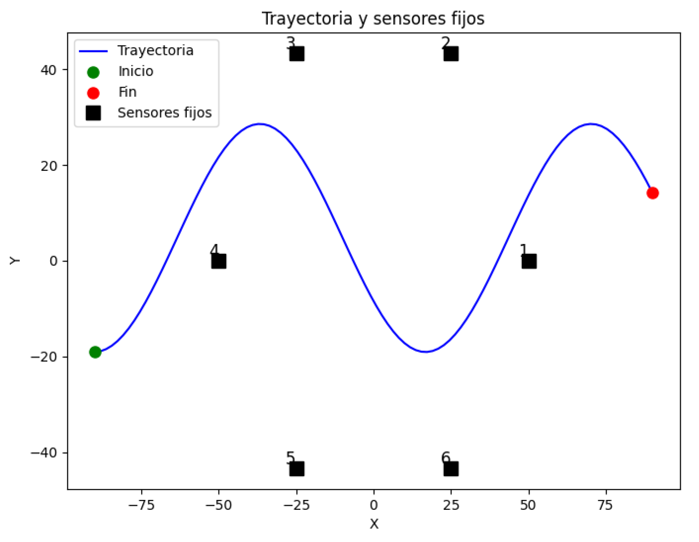
Unless otherwise stated, we emulate N s = 6 tri-axial fluxgates placed on a radius-50 m ring centred at the world origin (Figure A1). To study robustness against sensor dropout, we derive additional data by column deletion: we sequentially eliminate sensors, obtaining five- and four-sensor variants with an identical trajectory footprint. In future works we can assess whether using multi-component magnetic inputs ( B x , B y , B z ) further improves performance relative to the current Δ B z -only inputs.
  • Trajectory set:
For each of the 16 different field configurations, we generate 100 sinusoidal tracks, totalling 1600 simulated trajectories. Each time point in each trajectory contains the position of the vessel (the corresponding x , y coordinates), as well as a corresponding magnetic field measurement for each sensor. We do not inject sensor, installation, or sea-state noise in these simulations; results therefore reflect the noiseless AMPERES fields.

3.2. Task Taxonomy

We cast vessel localization as a task family T = T depth T size T sensors . Each task corresponds to a training–testing split. Since we have four different possible values for each of the main parameters, Depth ( in Meters ) = { 7.5 , 10 , 20 , 30 } , Vessel Size ( in Meters ) = { 2 × 1 , 4 × 2 , 8 × 4 , 20 × 10 } , and Number of sensors = { 3 , 4 , 5 , 6 } , that would yield 64 possible sets of combinations. In order to focus the scope of the project, we decided to center on the following combinations of parameters to define our In-Distribution Tasks and our Out-of-Distribution Tasks:
  • Depth tasks ( T depth ): To define this task, we decided to fix the hull size at 8 × 4 m, and the number of available sensors to N s = 4 , then we took the corresponding datasets with depths of { 7.5 , 10 , 20 } m which define our in-distribution (ID) for the T depth task; a 30 m depth constitutes the out-of-distribution (OOD) probe.
  • Size tasks ( T size ): In this second task, we fixed the depth as 20 m, and the number of sensors as N s = 4 sensors, taking the corresponding datasets of hull sizes { 2 × 1 , 4 × 2 , 8 × 4 } m for the ID data; 20 × 10 m is the OOD probe.
  • Sensor-drop tasks ( T sensors ): For the last task we tested, we fixed the vessel size as 8 × 4 m and depth as 20 m; our sensor subsets were four, five, and six sensors, and the extreme three-sensor case is our OOD data for this task. The order of sensor dropping wasas follows: first drop sensor 1, then sensor 3, and lastly sensor 5. It was carried out this way to retain as much triangulation capabilities as possible (see Figure A1).
We defined In Distribution and Out of Distribution in this way in order to test the capabilities of the approaches we test to generalize to data it has not seen before for that task. The resulting benchmark therefore challenges a model along three orthogonal factors: environmental variation (depth), target signature (size) and sensor availability, while guaranteeing a clean separation between adaptation (ID) and extrapolation (OOD) regimes. Note that OOD specifically denotes tasks that have never been seen during training, and hence, we use them to validate the generalization abilities of every method in this paper to previously unseen conditions.
  • Train/validation partition:
Within every task, trajectories are shuffled and separated 80 / 20 at the trajectory level so that validation tracks remain unseen during training. OOD datasets are never presented during training; they are reserved for the evaluation and generalization tests reported in Section 5.

4. Methods

4.1. Task-Specific MLP Baselines

  • Multilayer Perceptron Basics.
A multilayer perceptron (MLP) is a feed-forward neural network that stacks affine transforms and pointwise non-linearities. Its lineage traces to Rosenblatt’s single-layer perceptron [17]; practical multilayer training became feasible with the back-propagation algorithm introduced by Rumelhart et al. [18]. Theoretical work later showed that a feed-forward network with at least one hidden layer and non-polynomial activation is a universal approximator on compact domains [19]. Modern implementations benefit from rectifier-aware initialization schemes such as He (Kaiming) initialization [20], high-performing activations like GELU [21], and adaptive optimizers such as Adam [22].
  • Our baseline architecture.
Figure 1 illustrates the 6–128–128–2 MLP used as the base template in all deterministic baselines. Only high-level layer blocks are drawn; each layer is fully connected. A more detailed explanation of the MLP architecture can be seen in Appendix B.
  • Specialisation strategy.
To reveal the cost of over-specialising to a narrow operating regime, we train separate MLPs that each optimise along a single factor (depth, hull size, or number of active sensors). Each network sees data only from its designated parameter value; consequently, it can fit that regime well yet has no incentive to generalise. The three groups are as follows:
(a)
Depth MLPs: fixed hull of 8 × 4 m and N s = 4 sensors, with one model per depth in { 7.5 , 10 , 20 } m.
(b)
Size MLPs: fixed depth of 20 m and N s = 4 sensors, with one model per hull size in { 2 × 1 , 4 × 2 , 8 × 4 } m.
(c)
Sensor MLPs: fixed hull of 8 × 4 m at 20 m depth, with one model per active-sensor count in { 6 , 5 , 4 } .
These specialised MLPs allow us to (i) measure an upper-bound oracle performance within each narrow regime and (ii) perform cross-scenario stress tests by evaluating a model outside the conditions it was trained on (e.g., the 7.5 m depth model at 20 m), thereby quantifying brittleness.
Table 1 enumerates the models and training trajectory counts. A complementary domain-randomized alternative that aggregates data across settings is introduced in Section 4.2.
  • Inference use cases.
We employ these specialised MLPs in two complementary roles:
1.
Upper-bound oracle: Within their own scenario, they approximate the best MAE attainable with a lightweight feed-forward regressor (no uncertainty; no meta-adaptation).
2.
Cross-scenario stress test: When evaluated outside their training regime, they expose the brittleness of deterministic, over-specialised models, providing a stringent foil for the ANP’s meta-generalisation (Section 5).
  • Limitations of the MLP baseline and how the ANP addresses them.
The reference baseline [16] is a feed-forward MLP trained on simulated magnetic fields from a fixed seabed array. As formulated, it (i) is scenario-specific and typically requires retraining when sensor positions or scenario parameters change (hindering portability across hull/depth conditions), (ii) yields deterministic point predictions with no predictive uncertainty, and (iii) provides no mechanism to adapt at test time under domain shift. In contrast, our ANP casts localization as stochastic function regression: it cross-attends to a variable-size context of sensor–pose pairs and fuses this with a global latent code, enabling few-shot, gradient-free adaptation at inference and a Gaussian predictive distribution (mean and well-calibrated variance) [6,11]. These properties remove the need for on-device retraining, naturally accommodate variable sensor subsets, and improve the robustness under shift by conditioning on a handful of in situ context observations.

4.2. Domain-Randomized MLP Baselines (DRS)

A straightforward hedge against covariate shift is to expose a single regressor to the range of conditions it may encounter at test time, the domain randomization paradigm [7]. Rather than training separate networks per setting (Section 4.1), we therefore construct domain-randomized search baselines that pool data across multiple parameter values. We consider two granularity levels:
  • Task-aggregated DRS models. Three models each aggregate the in-distribution (ID) trajectories for a single factor:
    • DRS_depth: depths { 7.5 , 10 , 20 } m; hull 8 × 4 m; N s = 4 sensors.
    • DRS_size: hulls { 2 × 1 , 4 × 2 , 8 × 4 } m; depth 20 m; N s = 4 .
    • DRS_sensors: sensor counts { 6 , 5 , 4 } ; hull 8 × 4 m; depth 20 m.
    Each sees 300 trajectories (the union of the three specialised datasets in its group as seen in Table 2).
  • Global DRS-general model. One model ingests the entire ID corpus spanning all nine scenario combinations defined in Section 3.2: depths { 7.5 , 10 , 20 } m × hulls { 2 × 1 , 4 × 2 , 8 × 4 } m × sensor counts { 6 , 5 , 4 } channels. This totals 2700 trajectories ( 2.7 × 10 5 input–target pairs), an order of magnitude more data than any single specialised model.
  • Architecture.
All DRS variants reuse the baseline MLP of Figure 1 (6–128–128–2 with GELU activations). No architectural changes are made; only the training corpus differs.
  • Training protocol.
For each DRS model we aggregate the relevant ID trajectories, shuffle (at the sample level) within the training split, and apply the same 80/20% trajectory-level split used for the specialised models to prevent temporal leakage. Training hyper-parameters (optimizer, learning rate schedule, early stopping criterion) are held constant across all MLP baselines to isolate the impact of dataset breadth.

4.3. Attentive Neural Process

For one trajectory, we observe a time-ordered set D = { ( x t , y t , B t ) } t = 1 T , where x t , y t R 2 are the corresponding vessel position coordinates and B t R L is the vector magnetic measurements coming from the sensors (L is the number of sensors). During meta-training, a random split C D of | C | = M context points is disclosed; the learner must infer the target set T = D C . At test time, the operator is free to choose M, e.g., the first 30% of a track. This percentage used as context is always selected from the beginning of the trajectory, trying to mimic how real data from a marine vessel would be received and used. Other options of using context for these kinds of models suggest sampling randomly along the whole trajectory, but in our case, that would not be a realistic scenario.
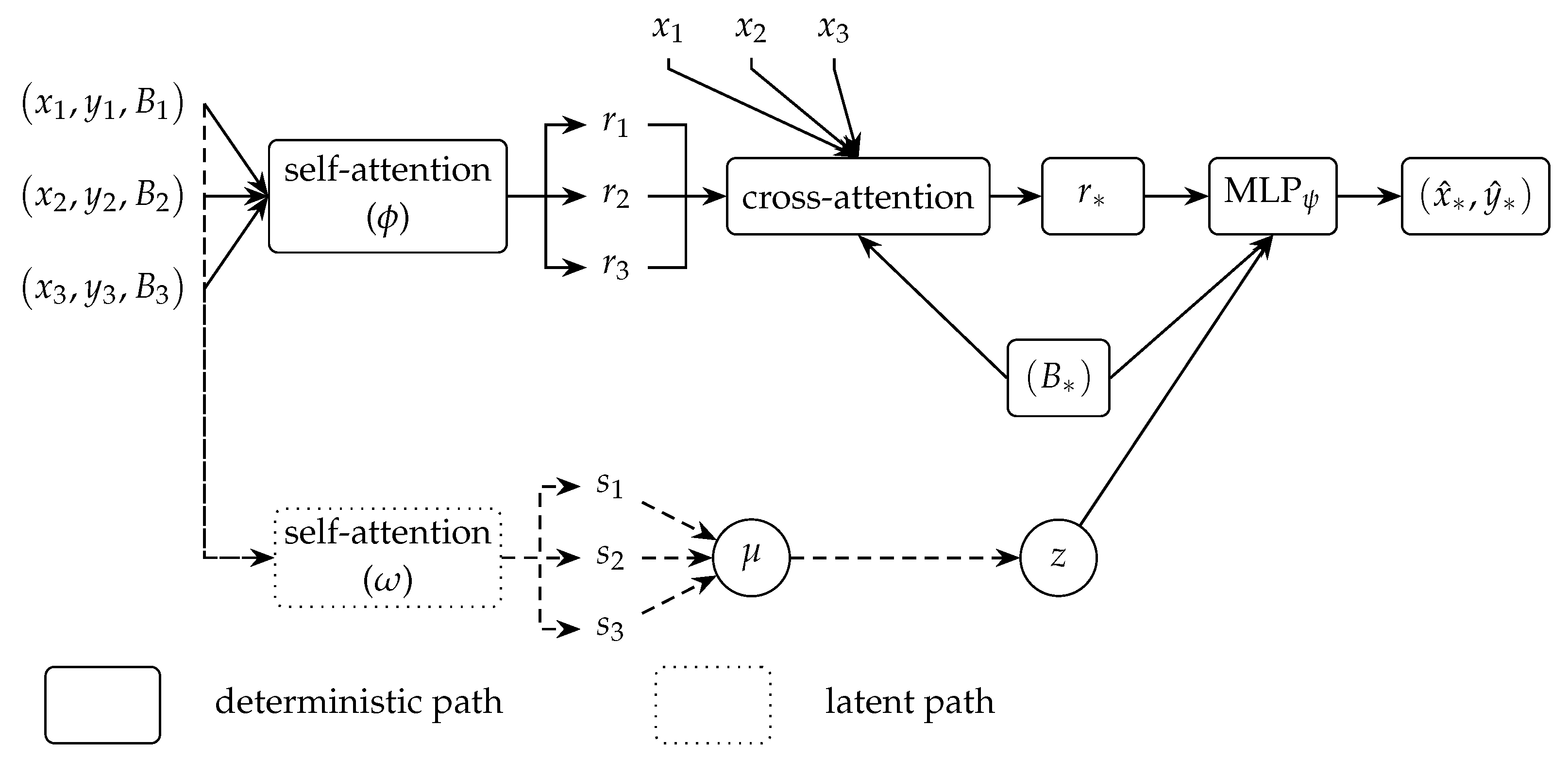
The ANP models the unknown mapping f : B ( x , y ) as a stochastic process conditioned on the context; its key components appear in Figure 2, and are detailed next.
(i)
Deterministic encoder
The encoder first embeds the context pairs and then lets each query point B q R L attend to C to predict ( x q , y q ):
r q = MHA Q = W Q B q , K = W K B C , V = W V [ B C , P C ] R H ,
where [ · , · ] denotes concatenation and MHA is multi-head attention with H hidden units and P C = ( x c , y c ) . Intuitively, r q summarizes which context sensors carry information most similar to the current reading B q . Let M = | C | be the number of context points. With L magnetometer channels and a hidden size H, the tensors involved in the cross-attention block of Equation (1) have the following dimensions:
B q R L W Q R L × H Q R 1 × H , B C R M × L W K , W V R L × H K R M × H V R M × H
The multi-head attention (MHA) module maps ( Q , K , V ) r q with r q R 1 × H , which we subsequently treat as a length-H row vector ( r q R H as written in (1)). In previous works, the attention mechanism of the Attentive Neural Process model has been explained as a general estimator [23].
(ii)
Latent encoder
Context alone seldom reveals the vessel identity or environmental bias. For every context index i { 1 , , M } , a two-layer MLP ω θ outputs a pair of D z -dimensional vectors μ i , log σ i 2 . The sub-script i labels the i-th context point. Their averages across i (following the methods used by Kim et al. [6]) yield the parameters μ ¯ , σ ¯ 2 R D z used in the Gaussian posterior:
q θ ( z C ) = N μ ¯ , diag σ ¯ 2 , z R D z .
The latent variable z acts as a compact code “fingerprint” of the current vessel–environment combination and is shared by all queries.
(iii)
Decoder
Given r q , the raw query (the L-dimensional vector B q of magnetic values from which we want to predict the position) and a sample z q θ , the decoder produces a Gaussian over the unknown position:
( μ q , log σ q 2 ) = ψ θ [ B q , r q , z ] , p θ ( x q , y q B q , C ) = N μ q , diag σ q 2 ,
where B q R L is the target-point magnetometer snapshot, r q R H is the deterministic attention summary for B q , z R D z is the global latent code for the current trajectory, [ B q , r q , z ] is the concatenated decoder input, μ q R 2 is the predicted mean position ( x ^ , y ^ ) , σ q 2 R 2 is the element-wise variance estimates and multi-head attention that thus handles local alignment, and N ( · ) indicates Gaussian (normal) distribution. z injects global context, yielding both accuracy and calibrated uncertainty.
The main reasoning is that the encoder is able to extract information about the task, which is then used by the decoder to adapt to this task. The decoder ψ θ maps its input to the mean and (log-)variance of a 2D Gaussian, and the predictive distribution over the unknown position ( x q , y q ) is exactly that Gaussian.
(iv)
Training objective-evidence lower bound.
For a single trajectory, we maximize the ELBO,
L ANP = 1 | T | q T log p θ ( x q , y q B q , C , z ) + KL q θ ( z D ) p θ ( z C ) ,
and the KL regulariser follows the conditional-VAE formulation of Neural-Process models [6,24], pushing the posterior q θ ( z D ) towards the context-dependent prior p θ ( z C ) ; this ensures that z captures only the residual information that is absent from the deterministic (attention) path, as already argued, sometimes implicitly, in those works and in the original VAE derivation [25].
(v)
Context-target sampling and batching.
At each optimization step, we draw context points uniformly from 10% to 50% ( M U { 10 , , 50 } ) out of the total T = 100 points each trajectory has to build C .
The resulting ANP combines (i) few-shot adaptability via z , (ii) context-aware matching via cross-attention, and (iii) probabilistic outputs for downstream risk-aware planning.

5. Results

This section quantifies the localization performance of the proposed Attentive Neural Process against the strongest deterministic baseline, the domain-randomized search feed-forward network (DRS-general), and various sets of specialized MLP models tested in different experiments. We try to always focus on the most demanding setting, cross-configuration generalization, by comparing the MAE per scenario. We remark that ANP and DRS-general were trained once and validated under different scenarios, contrary to single-task MLPs, where we train a single MLP per task.

5.1. Statistical Analysis

To judge whether the performance gaps reported in the following sections are merely due to chance, we adopt the two-stage, rank-based procedure recommended by Demšar [26] and summarised in the survey of Rainio et al. [27]. All tests are carried out on the MAE scores for every (model, dataset) pair inside each task family (depth, size, and sensors).
  • Step 1—omnibus test.
For every task, we first apply the Friedman–Iman–Davenport test: each method is replaced by its rank on each dataset (lower MAE ⇒ better rank), and the resulting rank matrix is fed to the Friedman statistic, with the Iman–Davenport F correction to account for the modest number of datasets. If the null hypothesis of “equal performance” is not rejected at the α = 0.05 level, no further comparisons are made.
  • Step 2—pairwise follow-up.
Whenever the omnibus test is significant, we perform paired Wilcoxon signed-rank tests that compare every competitor against the model that attains the best average rank. Because multiple pairwise tests inflate the family-wise error rate, the resulting p-values are adjusted with the Holm step-down procedure; only adjusted values below α are declared significant.
This two-stage, fully non-parametric protocol (i) requires no distributional assumptions on the MAE scores, (ii) controls the overall probability of Type-I errors, and (iii) follows the best-practice guidelines put forward by Demšar [26] and Rainio et al. [27].

5.2. ANP vs. DRS-General on ID and OOD Tasks

We first want to compare the two models that are trained only once on all tasks, namely, ANP and DRS-general, in order to compare their performance. We evaluated these models in the validation split of the 9 scenarios that were seen during training. These are composed of the 2700 trajectories from all the possible combinations of the in-distribution data of the tasks described in Section 3.2.
  • Quantitative results
Table 3 presents the results in terms of the mean MAE obtained by each of the models in that specific dataset. We also provide color-coded heat maps in Figure A2 (Appendix C.1) that contain the same information.
We can clearly see that our proposed ANP model is significantly better than DRS-general. This is statistically backed by checking the corrected Wilcoxon p-values in Table 4. From Table 3 and Table 4, we also see that our ANP approach almost halves the error rate in many of the scenarios tested.

5.3. Depth Ablation

We now proceed to a more detailed ablation for each of the task dimensions of our experiments (depth, hull size, and number of sensors), as well as testing the generalization capabilities of our models by using the OOD data, never seen during training, for validation. We start with the submersion depth that determines the vertical stand-off between the ferromagnetic hull and the seabed sensor plane; the larger that distance is, the weaker and smoother the magnetic anomaly becomes. Vessels can transition from shallow littoral waters down to deeper layers, so a deployable localiser must compensate for signal attenuation without site-specific re-training. To isolate this factor in this test, we keep (i) the hull dimensions fixed at 8 × 4 meters and (ii) use the four-sensor configuration, then carve four depth-specific subsets:
  • 7.5 m, 10 m, 20 m in-distribution: depths seen during training.
  • 30 m → out-of-distribution: an extrapolation stress-test never shown to the models.
  • Models under test
Three single-depth MLPs (MLP_7-5m, MLP_10m, and MLP_20m) are trained only on their respective ID subset (100 trajectories). DRS_depth is trained on the union of the three (300 trajectories), which represents a domain-randomized model specialized in this task, while DRS_general and the proposed ANP are the same global models trained in Section 5.2.
  • Quantitative results
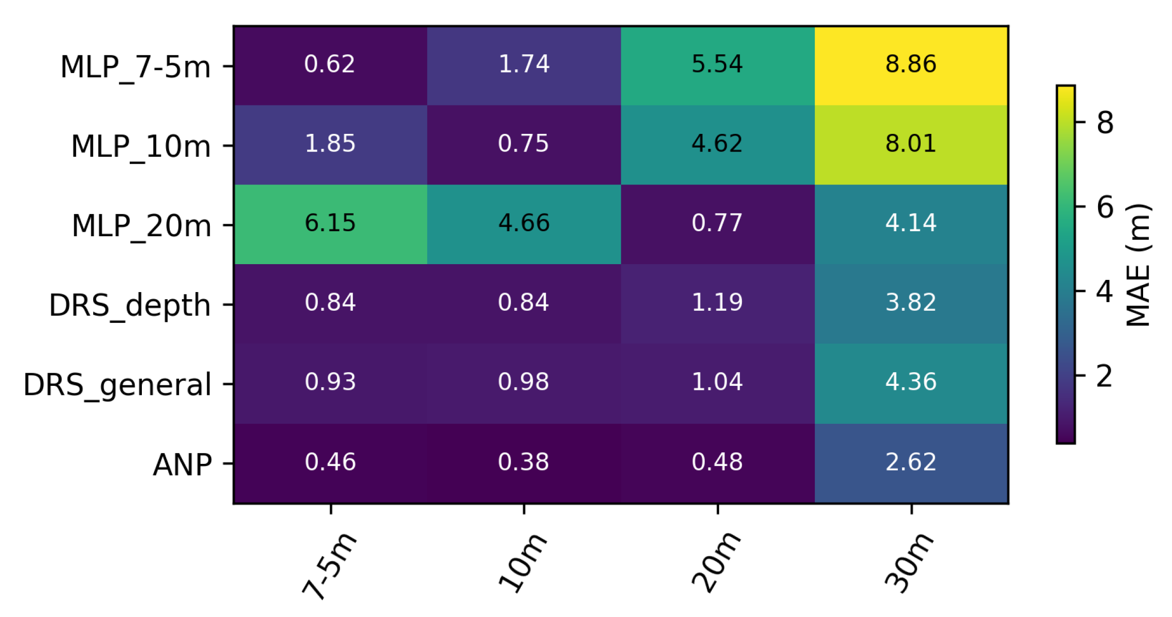
Table 5 reports the mean absolute error (in meters) for every model-depth pair; the best entry per column is bold-faced. Table 6 provides Wilcoxon and Friedman–Holm statistics against the ANP baseline. A color heat-map is shown in Appendix C.2, Figure A4, for visual comparison.
The single-depth MLPs illustrate the classic bias-variance trade-off: each is highly accurate in its native depth (0.62 m at 7.5 m, 0.75 m at 10 m, 0.77 m at 20 m) but their MAE grows up to 13 × when evaluated outside that band. DRS_depth, trained on mixed depths, is more robust yet still trails the ANP in all four columns of Table 5. The ANP not only attains the lowest error across the three ID depths but also preserves around a 32 % margin over the best deterministic alternative in the unseen 30m case. Table 6 confirms statistical significance: all single-depth MLPs are inferior to the ANP after Holm correction ( p < 0.05 ), whereas the gap between DRS_depth and the ANP is not significant, likely due to having only four datasets in the test, although the p-value is nonetheless low (<0.1 in all cases).

5.4. Hull-Size Ablation

The vessel’s volume, approximated here by its length × width rectangle, directly scales the dipole moment that perturbs the ambient field. A localiser tuned to a small vessel may therefore saturate or mis-scale when confronted with a larger hull, and vice versa. To isolate this factor, we lock the depth at 20 m and took the corresponding four-sensor ring datasets, then create three in-distribution subsets with increasing hull sizes:
  • 2 m × 1 m (small), 4 m × 2 m (medium), 8 m × 4 m (large),
and an out-of-distribution subset 20 m × 10 m that represents the magnetic signature of a larger vessel.
  • Models under test
Three single-size MLPs (MLP_2 × 1 m, MLP_4 × 2 m, and MLP_8 × 4 m) are specialized to their respective ID subset; DRS_size is trained on the union of the three. DRS_general and the proposed ANP are the same global models evaluated previously.
  • Quantitative results
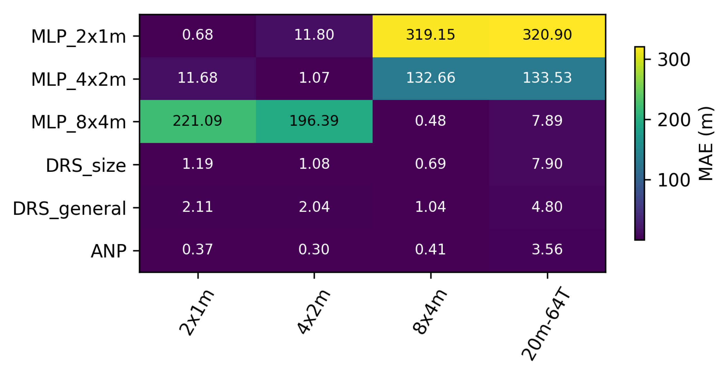
Again we presented the results in Table 7 which reports the MAE in meters for every model–size pair, and Table 8 which summarizes Wilcoxon/Friedman significance tests against the ANP baseline. The color heat-map is provided in Appendix C.3, Figure A5.
Each single-size MLP attains sub-1m accuracy on its training hull (Table 7) but collapses by two orders of magnitude when confronted with a different magnetic cross-section (e.g., from 0.68 m to 319 m moving 2 × 1 m → 8 × 4 m). Task-specialized domain randomization (DRS_size) mitigates the worst failures but still lags behind the ANP by 2 × on the OOD 20 × 10 m hull. For the Friedman p-value in Table 8, the consistent column-wise wins and the ANP’s lower mean error (1.16 m) indicate superior robustness to unseen magnetic amplitudes. Again, this suggests that an ANP-based localiser would require fewer re-calibration samples when commissioning a vehicle class outside the original training envelope. In general, we again observe low p-values (<0.1).

5.5. Sensor Count Ablation

Sea-going magnetic arrays may be affected by axis dropouts due to various factors: salt-water ingress, connector corrosion, or fluxgate saturation can disable one or more channels during a mission. A localization model that relies on a fixed, full set of inputs may therefore fail abruptly when a single sensor goes offline. To quantify robustness, we hold both hull size (8 m × 4 m) and depth (20 m) constant and vary only the number of active magnetometers:
  • 6 s, 5 s, 4 s—three in-distribution subsets in which zero, one, or two sensors are disabled at the same time;
  • 3 s—an out-of-distribution subset that removes a third channel, emulating a more severe hardware failure.
  • Models under test
Each ID subset receives its own lightweight perceptron (MLP_6s, MLP_5s, or MLP_4s). DRS_sensors pools the three ID datasets. The global DRS_general and our ANP are reused without re-training.
  • Quantitative results
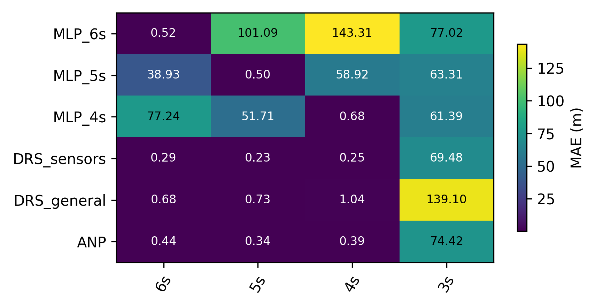
Table 9 presents the corresponding obtained MAE in meters; Table 10 lists Wilcoxon/ Friedman statistics. Appendix C.4, Figure A6, visualizes the same data as a heat map.
As seen in the previous tests, each single-count MLP excels only when presented with the exact sensor layout it was trained on, but its MAE explodes, by up to two orders of magnitude, whenever channels are missing. In-domain aggregation (DRS_sensors) yields the best overall accuracy for 6-4 sensors and still degrades gracefully at 3 s (69 m MAE). The ANP is competitive with DRS_sensors on every ID column and, crucially, maintains sub-75 m error in the extreme three-sensor OOD case despite never having seen so few inputs. Although the Friedman test lacks power with just four datasets, the Wilcoxon comparison flags MLP_6s as significantly worse than the ANP ( p Holm = 0.0245 ), illustrating how brittle a deterministic, sensor-specific pipeline can be.
Overall, the ANP’s encoder-decoder design appears to learn an implicit “missing-channel” prior, enabling robust localization even under severe hardware degradation, and despite not being the outright best, a large p-value of 0.45 (Table 10) indicates that it is close in performance to the best model.

5.6. Unified Cross-Task Benchmark

The previous ablation studies evaluated each generative factor (depth, hull size, sensor count) in isolation. In a real deployment, however, the learning system may have to contend with simultaneous variation along all three axes. We therefore ran a final holistic benchmark that loads all available models, the nine task-specialised MLPs, the three task-specific domain-randomized networks, the global DRS_general, and the proposed ANP, and tests them on the complete set of twelve trajectory collections ( 3 × depth ID + 3 × size ID + 3 × sensors ID + 3 OOD probes).
The resulting 14 × 12 MAE matrix (shown as a Table A2 in Appendix C.5) condenses 14 models × 12 datasets = 168 evaluations executed with the common harness described previously. We include the summary of the statistics obtained in Table 11.
Four clear patterns emerge: 1. ANP dominates across all contexts. Its average error (6.6 m) is roughly half that of the next best competitor (DRS-general, 13.2 m) and an order of magnitude below most single-scenario MLPs. 2. Statistical significance is strong. Holm-corrected Wilcoxon tests reject every alternative model versus the ANP ( p < 0.025 ), and Friedman post-hoc confirms the ranking ( p < 0.05 ) for all but two cases. 3. Over-specialised MLPs collapse out-of-domain. Models such as MLP_10m soar from 0.66 m 840 m MAE when depth changes (Table 11), inflating their mean error to >200 m. 4. Domain randomization helps but is insufficient. The three task-specific DRS baselines improve stability but still trail the ANP by factors of 2–10×, illustrating that set-conditional adaptation is crucial.

5.7. Trajectory-Level Extrapolation: ANP vs. DRS-General

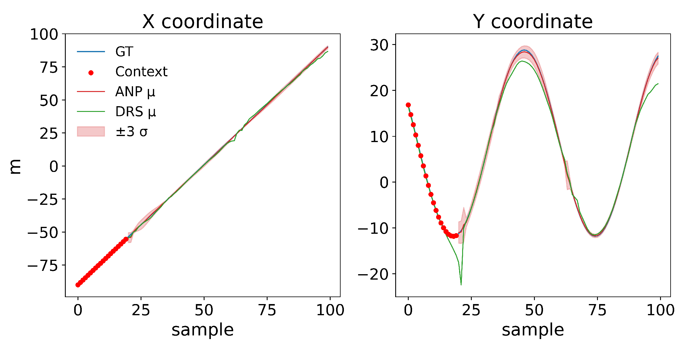
To illustrate the extrapolation capability of the ANP, this trajectory experiment isolates a single held-out track from the 20 m depth, 8 × 4 m hull, four-sensor setting and splits it 20%/80% in time. The first fifth of the samples ( M = 20 ) are supplied to each model as context; the remainder must be predicted. We compare the stochastic ANP, which returns a mean path μ and per-frame standard deviation σ, and the deterministic DRS-general MLP.
Figure 3 reveals three key behaviours: ( i ) Faithful continuation: After the context window, the ANP mean (red) follows the ground-truth sinusoid almost perfectly in both the monotonic x component and the oscillatory y component. The DRS-general curve (green) begins to drift after the first crest and undershoots subsequent peaks. ( i i ) Calibrated confidence: The ANP’s ± 3 σ band widens exactly where curvature is largest (tops and troughs of the sine wave) and narrows over the linear sections, matching intuitive signal difficulty. In every frame, the blue trace remains inside the pink envelope, indicating well-calibrated uncertainty. DRS-general, being deterministic, offers no such measure. ( i i )  Error containment: The maximum absolute deviation of ANP from ground truth is never too large in y; DRS-general accumulates a larger error by the end of the trajectory.
These observations corroborate the aggregate statistics of Section 5.3, Section 5.4 and Section 5.5: the latent-variable and cross-attention design not only lowers MAE on average but also delivers actionable per-sample credibility estimates, enabling downstream planners to hedge when the positional error distribution broadens.

5.8. Results Discussion

The experiments reported in this section lead to three main conclusions:
(a)
ANP consistently achieves the lowest MAE across all settings. In every in-distribution scenario (Table 3), the ANP improves over the deterministic baseline DRS-general by nearly 50% on average (0.43 m vs. 0.84 m MAE). It also retains a clear advantage in all out-of-distribution tests. The difference of the ANP against all other methods is statistically very significative, as seen in Table 11. Also, the fact that this approach provides uncertainty σ values, gives us the important advantage of having an interval to perform our localization.
(b)
Task-specific MLPs excel only in their training domain. As shown in the depth, size, and sensor ablation studies (Table 5, Table 6, Table 7, Table 8 and Table 9), each specialized MLP performs well on its target dataset but fails to generalize, often showing errors one to two orders of magnitude higher in other settings (e.g., hull-size extrapolation).
(c)
Domain randomization is not sufficient. While DRS-general is more robust than single-task MLPs, it still lags behind ANP by roughly 2 × in some ID scenarios and over 3 × in some OOD scenarios. Conditioning on a small, trajectory-specific context at test time, as ANP does, proves to be substantially more effective than a global set of weights alone.
The statistical tests in Table 6, Table 8 and Table 10 reinforce these observations: whenever the Friedman test rejects the null hypothesis, the Holm-corrected Wilcoxon post-hoc test confirms the ANP’s superiority. While differences in the size and sensor ablation tasks follow the same pattern, their limited number of tasks prevents achieving strong statistical significance. This was solved in the experiment in Section 5.6, where the combination of all tasks and methods provided us with a sample size big enough to back up the statistical significance of our results.
From a practical deployment perspective, our ANP also presents some advantages:
(i)
Few-shot adaptability: The ANP matches and even surpasses the accuracy of oracle-like MLPs with only a handful of labelled samples, avoiding costly retraining cycles.
(ii)
Robustness to sensor failure: In the three-sensor OOD test, the ANP maintains errors around 70 m MAE (Table 9), comparable to specialized single-task MLP and DRS_sensors.
(iii)
Low inference latency: A single forward pass of the ANP (20 context points + 80 targets, B = 1 ) takes approximately 3.8 ms on an RTX 2080 Ti (FP32). Scaled estimates suggest about 38 ms in FP32 or 9 ms in FP16/TensorRT on Jetson Xavier NX, and 110 ms in FP32 on Jetson Nano Appendix D), which means that our procedure could be implemented in real-time estimation applications with low-cost hardware.

6. Conclusions and Future Work

This study introduces, for the first time, Attentive Neural Processes as a meta-learning framework for passive magnetic-anomaly localization. By viewing the mapping from six tri-axial magnetometer readings to a horizontal position as a family of functions that depends on the vessel signature, sensor layout, and environmental context, the ANP can adapt to a previously unseen configuration after observing only a handful of context points, without any test-time back-propagation. When trained on a richly domain-randomized simulator, the proposed model attains the same accuracy as highly specialized multilayer perceptrons within their calibration domains and reduces mean absolute error by up to 50% when forced to extrapolate across hull sizes, depths, or sensor dropouts. In addition, the predictive variance produced by the ANP is well calibrated, enabling downstream planners to reason about localization confidence in real time.
We remark that we train our ANP model once, and then validate over an extensive set of benchmarks, where its adaptability is shown to be superior to the rest of the methods tested, even to conditions unseen during training.
These results point to Neural-Process meta-learning as a practical and scalable route towards confidence-aware magnetic navigation systems that must cope with heterogeneous vessel signatures, intermittent sensor failures, and non-stationary operating conditions. The combination of zero-gradient adaptation, principled uncertainty, and millisecond inference time makes ANPs an appealing alternative to both classical Bayesian filters and fixed neural networks.

Future Work

Despite these encouraging findings, three avenues remain open: (i) synthetic-to-real transfer, Earth-field orientation, and multi-component sensing. The present study relies exclusively on simulated magnetic fields; real-world seawater disturbances, soft-iron bias, and sensor drift were not modeled. A natural next step is to design a small sea trial and curate field datasets that capture geomagnetic inclination/declination (e.g., via the World Magnetic Model [28]), installation offsets, wave-induced motion, and electromagnetic interference. Within this setting we will (a) quantify how many context points the ANP needs for in situ commissioning, (b) evaluate multi-component magnetic inputs ( B x , B y , B z ) versus the current Δ B z channel, and (c) study sim-to-real strategies that preserve our no-retraining-at-deploy time constraint, such as domain randomization augmented with adversarial domain adaptation [29,30] and small, offline fine-tuning prior to deployment. (ii) Three-dimensional sensor constellations. All experiments assumed a planar ring of fluxgates. Extending the architecture to irregular 3D arrays, such as towed gradiometers or hull-mounted clusters, will require positional encodings that respect full spatial geometry and may benefit from graph-based message passing. (iii) Multi-target and cluttered scenes. The current pipeline tracks a single vessel against a geomagnetically “clean” background. Real deployments must disentangle multiple, possibly overlapping signatures amid crustal anomalies and anthropogenic noise. Hierarchical or multi-output Neural Processes [31,32], combined with sequential data association, offer a promising research direction to segment and track several dipoles simultaneously.
Addressing these challenges will further close the gap between simulation and practice and could establish ANPs as the backbone for future passive localization suites in marine robotics and naval surveillance.

Author Contributions

Conceptualization, L.F.F.-S., B.V.T. and J.P.; methodology, L.F.F.-S., B.V.T., A.A. and J.P.; software, L.F.F.-S. and J.P.; validation, L.F.F.-S., B.V.T. and J.P.; formal analysis, L.F.F.-S., B.V.T. and J.P.; investigation, L.F.F.-S., A.A. and J.P.; resources, J.P.; data curation, L.F.F.-S. and B.V.T.; writing—original draft preparation, L.F.F.-S. and B.V.T.; writing—review, and editing, A.A. and J.P.; visualization, L.F.F.-S., B.V.T. and J.P.; supervision, A.A., J.P. and S.Z.; project administration, J.P. and S.Z.; funding acquisition, J.P. and S.Z. All authors have read and agreed to the published version of the manuscript.

Funding

This research was funded by the Spanish Ministry of Science, Innovation and Universities, the National Research Agency (10.13039/501100011033) and the European Regional Development Fund under the grant PID2023-146540OB-C42 (NEMO4EX).

Data Availability Statement

The study did not involve any new empirical data collection. All data used are synthetic and were generated using the described simulation pipeline in Section 3.1. The original contributions presented in this study are included in the article. Further inquiries can be directed to the corresponding author. Along with the trajectory data, our code and data are publicly available to foster reproducibility and future research in https://github.com/FernandoFS96/tesis/tree/c42b6b10f03a7c8f9f352fe8f8c7cae55069ab5a/magnetic-localization (Github) (accessed on 19 August 2025).

Conflicts of Interest

The authors declare no conflicts of interest. The funders had no role in the design of the study; in the collection, analyses, or interpretation of data; in the writing of the manuscript; or in the decision to publish the results.

Appendix A. Dataset Construction

Appendix A.1. Sensor Geometry

To emulate a realistic magnetic array, we place six virtual flux-gate magnetometers on a circle of radius R = 50 m . Their Cartesian coordinates are ( ± R , 0 ) and ( 0 , ± R ) , that is, the four cardinal directions, plus the two diagonal points ( R / 2 , R / 2 ) and ( R / 2 , R / 2 ) . All sensors lie on the same horizontal plane as the synthetic field map, so variations in the vertical component Δ B z are purely due to the simulated vessel rather than sensor height differences (physically, this plane represents a fixed seabed array).

Appendix A.2. Trajectory Generator

Each vessel path is a gently meandering line: the x-coordinate follows a sinusoid, while the y-coordinate grows linearly with time. Formally, for t [ 0 , 100 ] s ,
x ( t ) = x 0 + A sin ( ω t ) , y ( t ) = y 0 + v t .
The four trajectory parameters are drawn independently for every run:
A U 1 , 10 m , ω U 0.04 , 0.07 rad / s , v U 0.05 , 0.15 m / s , x 0 , y 0 U 5 , 5 m .
Sampling 100 distinct trajectories for each of the 16 hull-depth scenarios produce a benchmark suite of 1600 synthetic tracks.

Appendix A.3. Measurement Transform

Raw anomalies Δ B z span several orders of magnitude, so we stabilize their dynamic range with a signed-logarithmic map:
b scaled = sign ( b ) log | b | + ε ,
where ε is a small constant that preserves numerical stability near zero. The transform is applied to every sensor reading before the values are written to the CSV files that feed the learning pipeline.

Appendix A.4. Sensor Configuration

Figure A1. Example of the disposition of the sensor array in the trajectory space.
Jmse 13 01627 g0a1

Appendix A.5. Absolute ΔB Ranges

For each hull-depth configuration, we report the absolute minimum and maximum values of the AMPERES Δ B grid at the sensor plane. These values substantiate the statement in Section 3.1 that Δ B spans multiple orders of magnitude. Table A1 lists min/max per configuration.
Table A1. Absolute Δ B ranges at the sensor plane for all hull-depth configurations. Values are reported in nT (raw simulator units are Tesla).
Depth (m)Hull (m)N Δ B min Δ B max | Δ B | p 1 | Δ B | p 50 | Δ B | p 99 | Δ B | max
7.520 × 106328−277.10277.100.04820.5022147.20277.10
7.52 × 16328−169.00169.000.01130.100556.892169.00
7.54 × 26328−246.70246.700.01740.155087.140246.70
7.58 × 46328−1015.01015.00.07800.6977398.891015.0
10.020 × 106328−156.10156.100.06830.6481101.32156.10
10.02 × 16328−72.92072.9200.01490.130337.36372.920
10.04 × 26328−109.50109.500.02300.201056.766109.50
10.08 × 46328−468.70468.700.10310.9022255.42468.70
20.020 × 106328−32.32032.3200.10951.03227.71032.320
20.02 × 16328−2.5282.5287.055 × × 10 3 0.05822.0812.528
20.04 × 26328−14.24014.2400.03880.329311.76414.240
20.08 × 46328−63.11063.1100.17531.48452.23263.110
30.020 × 106328−11.29011.2900.10821.10910.44211.290
30.02 × 16328−0.75350.75356.885 × 10 3 0.06380.69100.7535
30.04 × 26328−4.2564.2560.03820.36043.9064.256
30.08 × 46328−18.98018.9800.17241.62017.44618.980
Percentiles are computed on | Δ B | . Units are nT; raw simulator units are Tesla.

Appendix B. Baseline MLP Architecture

Appendix B.1. Forward Mapping

Given sensor vector s = ( s N , s E , s S , s W ) , the network computes
h ( 1 ) = ϕ W ( 1 ) s + b ( 1 ) , h ( 2 ) = ϕ W ( 2 ) h ( 1 ) + b ( 2 ) , p ^ = W ( 3 ) h ( 2 ) + b ( 3 ) ,
where ϕ ( · ) = max ( 0 , · ) and p ^ = ( x ^ , y ^ ) .

Appendix B.2. Loss and Optimization

The network minimises L MLP = p ^ p 1 with Adam ( η = 5 × 10 3 ; see Appendix B.3 for all hyper-parameters).

Appendix B.3. MLP Baseline Hyper-Parameters

  • Architecture: 6-128-128-2 with GELU activations; He uniform initialization.
  • optimizer: Adam, η = 5 × 10 3 , β 1 , 2 = ( 0.9 , 0.999 ) .
  • Batch size: 500 samples.
  • Early stopping: patience 1000 on validation MAE; max 10,000 epochs.
  • Base MLPs: one model per scenario (100 samples each).
  • DRS MLP: same capacity, trained on concatenated 300 samples.

Appendix C. Evaluation Results

Appendix C.1. Heatmaps ANP vs. DRS-General
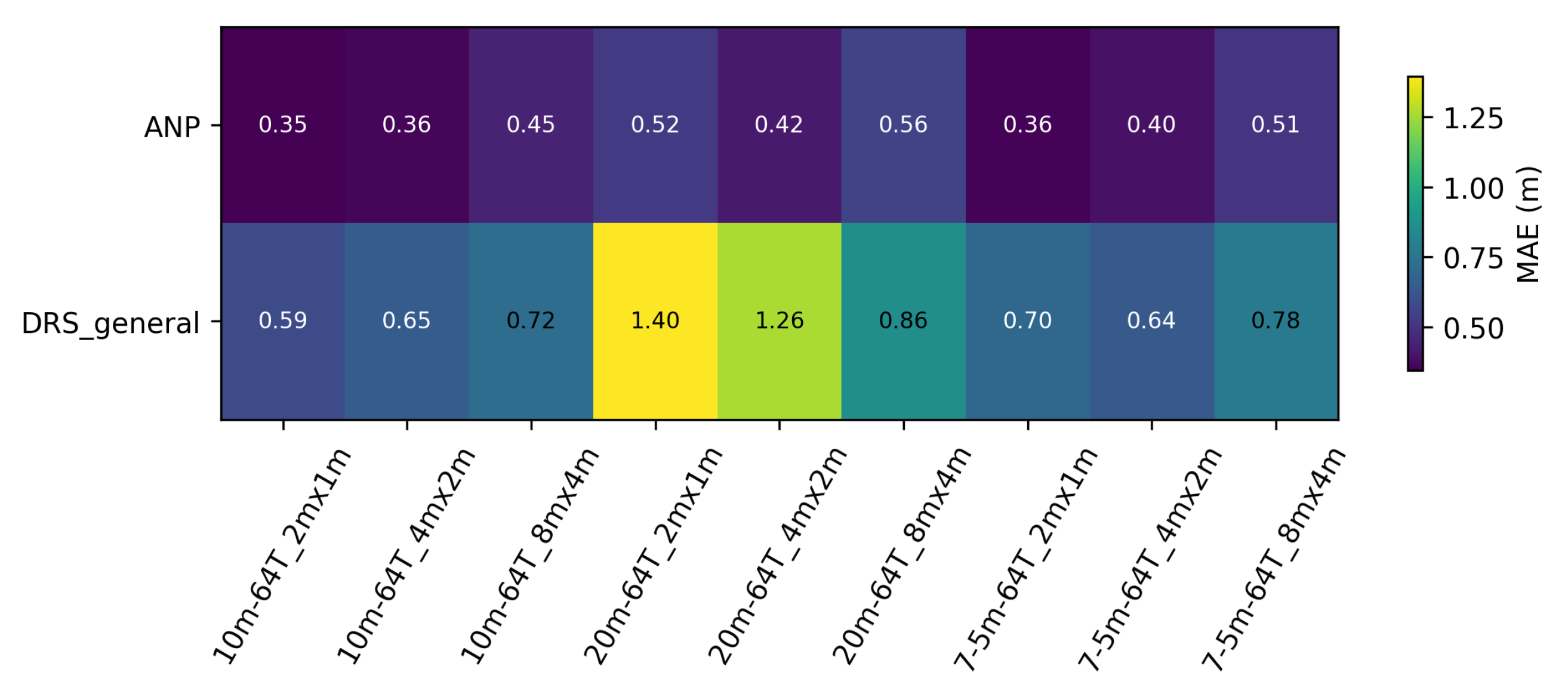
Figure A2. Per-scenario MAE heat-map for in-distribution validation set.
Jmse 13 01627 g0a2
Figure A3. Per-scenario MAE heat-map for out-of-distribution set.
Jmse 13 01627 g0a3

Appendix C.2. Heatmaps Task: Depth

Figure A4. Color-coded MAE heat-map for the depth experiment.
Jmse 13 01627 g0a4

Appendix C.3. Heatmaps Task: Size

Figure A5. MAE heat-map for the size experiment.
Jmse 13 01627 g0a5

Appendix C.4. Heatmaps Task: Sensors

Figure A6. MAE heat-map for the sensor experiment.
Jmse 13 01627 g0a6

Appendix C.5. Complete MAE Matrix for the Unified Benchmark

Table A2 lists the 14 × 12 = 168 mean absolute errors obtained when every model is evaluated on every dataset (three × depth, three × hull size, three × sensor count, plus the three OOD probes). These are the raw numbers underlying the statistical analysis in Section 5.6.
Table A2. Mean Absolute Error (m) of all 14 models on each of the 12 trajectory collections. Lower is better; best values per column are highlighted in bold.
Depth-7–5 mdepth-10 mdepth-20 mdepth-30 msize-2 × 1 msize-4 × 2 msize-8 × 4 msize-20 × 10 msens-6 ssens-5 ssens-4 ssens-3 s
ANP0.420.340.382.670.330.240.383.910.350.340.3869.66
DRS-general0.930.981.044.362.112.041.044.800.680.731.04139.10
MLP-7–5 m0.741.675.218.34199.64188.715.216.6867.5834.015.21109.34
MLP-10 m1.610.664.408.06958.86840.544.407.60124.8645.664.40433.72
MLP-20 m6.454.810.673.94135.73128.300.675.30100.0667.640.67126.07
DRS-depth0.880.831.514.11687.02641.541.515.46132.48145.681.5153.03
MLP-2 × 1 m328.56325.96319.15317.110.6811.80319.15320.90390.72395.22319.15425.03
MLP-4 × 2 m135.91135.38132.66129.9311.681.07132.66133.53141.52181.26132.66346.08
MLP-8 × 4 m6.844.990.483.59221.09196.390.487.89267.7681.660.4893.91
DRS-size6.574.690.693.911.191.080.697.90149.91140.700.6972.53
MLP-6 s144.38143.49143.31145.16206.65194.01143.31143.160.52101.09143.3177.02
MLP-5 s60.0659.9458.9259.29287.17253.5858.9260.4138.930.5058.9263.31
MLP-4 s6.564.920.684.08243.44218.310.685.7177.2451.710.6861.39
DRS-sensors8.866.360.254.03345.17320.200.257.570.290.230.2569.48

Appendix D. Latency Estimation on Embedded Devices

Appendix D.1. Reference Measurement on Our Server Desktop

  • Hardware & Software: NVIDIA RTX 2080 Ti (13.45 TFLOPS FP32) running PyTorch 2.2.
  • Script: test_latency.py scritp that performs N = 200 timed iterations after ten warm-up passes.
  • Result: t 2080 ti = 3.775 ms per batch ( 20 + 80 points, B = 1 , FP32).

Appendix D.2. Computational Scaling Model

The forward pass is dominated by matrix–matrix products in the decoder. Assuming identical kernel efficiency η across devices, latency scales inversely with sustained FLOPS ([33]):
t device t 2080 ti FLOPS 2080 ti FLOPS device η 2080 ti η device .
Various empirical studies show that Jetson Xavier NX reaches η device 0.35 (plain FP32) and ~0.65 with TensorRT/FP16; Jetson Nano sustains η device 0.30 under continuous load.

Appendix D.3. Device Specifications

Table A3. Compute capability used in Equation (A1).
DeviceArchitectureTFLOPS FP32TFLOPS FP16
RTX 2080 TiTuring TU10213.4527.0
Jetson Xavier NXVolta (384 CUDA)1.306.0
Jetson NanoMaxwell (128 CUDA)0.47

Appendix D.4. Resulting Latency Estimates

Table A4. Predicted single-batch latency for the ANP model.
DeviceModeScale FactorLatency
Jetson Xavier NXFP32 13.45 / 1.30 10.3 ~38 ms
Jetson Xavier NXFP16 (TensorRT) 27 / 6.0 4.5 ~9 ms
Jetson NanoFP32 13.45 / 0.47 28.6 ~110 ms

Appendix D.5. Limitations

(i)
Throttling on the Nano under passively cooled cases can add ∼20 % latency.
(ii)
Host ↔ device transfers are excluded.

References

  1. Zhang, S.; Yang, Y.; Xu, T.; Qin, X.; Liu, Y. Long-range LBL underwater acoustic navigation considering Earth curvature and Doppler effect. Measurement 2025, 240, 115524. [Google Scholar] [CrossRef]
  2. Alimi, R.; Fisher, E.; Nahir, K. In Situ Underwater Localization of Magnetic Sensors Using Natural Computing Algorithms. Sensors 2023, 23, 1797. [Google Scholar] [CrossRef]
  3. Gidugu, A.; Vandavasi, B.N.J.; Narayanaswamy, V. Bio-inspired machine-learning aided geo-magnetic field based AUV navigation system. Sci. Rep. 2024, 14, 17912. [Google Scholar] [CrossRef]
  4. Chen, X.; Hu, J.; Jin, C.; Li, L.; Wang, L. Understanding Domain Randomization for Sim-to-real Transfer. arXiv 2022, arXiv:2110.03239. [Google Scholar] [CrossRef]
  5. Muratore, F.; Ramos, F.; Turk, G.; Yu, W.; Gienger, M.; Peters, J. Robot Learning from Randomized Simulations: A Review. arXiv 2022, arXiv:2111.00956. [Google Scholar] [CrossRef] [PubMed]
  6. Kim, H.; Mnih, A.; Schwarz, J.; Garnelo, M.; Eslami, A.; Rosenbaum, D.; Vinyals, O.; Teh, Y.W. Attentive Neural Processes. arXiv 2019, arXiv:1901.05761. [Google Scholar] [CrossRef]
  7. Tobin, J.; Fong, R.; Ray, A.; Schneider, J.; Zaremba, W.; Abbeel, P. Domain Randomization for Transferring Deep Neural Networks from Simulation to the Real World. arXiv 2017, arXiv:1703.06907. [Google Scholar] [CrossRef]
  8. Heshmat, M.; Saoud, L.S.; Abujabal, M.; Sultan, A.; Elmezain, M.; Seneviratne, L.; Hussain, I. Underwater SLAM Meets Deep Learning: Challenges, Multi-Sensor Integration, and Future Directions. Sensors 2025, 25, 3258. [Google Scholar] [CrossRef]
  9. Cohen, K.M.; Park, S.; Simeone, O.; Shamai, S. Bayesian Active Meta-Learning for Reliable and Efficient AI-Based Demodulation. IEEE Trans. Signal Process. 2022, 70, 5366–5380. [Google Scholar] [CrossRef]
  10. Etiabi, Y.; Eldeeb, E.; Shehab, M.; Njima, W.; Alves, H.; Alouini, M.S.; Amhoud, E.M. MetaGraphLoc: A Graph-based Meta-learning Scheme for Indoor Localization via Sensor Fusion. arXiv 2024, arXiv:2411.17781. [Google Scholar] [CrossRef]
  11. Garnelo, M.; Schwarz, J.; Rosenbaum, D.; Viola, F.; Rezende, D.J.; Eslami, S.M.A.; Teh, Y.W. Neural Processes. arXiv 2018, arXiv:1807.01622. [Google Scholar] [CrossRef]
  12. Gordon, J.; Bruinsma, W.P.; Foong, A.Y.K.; Requeima, J.; Dubois, Y.; Turner, R.E. Convolutional Conditional Neural Processes. arXiv 2020, arXiv:1910.13556. [Google Scholar] [CrossRef]
  13. Song, J.; Bagoren, O.; Skinner, K.A. Uncertainty-Aware Acoustic Localization and Mapping for Underwater Robots. arXiv 2023, arXiv:2307.08647. [Google Scholar] [CrossRef]
  14. Wang, C. Calibration in Deep Learning: A Survey of the State-of-the-Art. arXiv 2024, arXiv:2308.01222. [Google Scholar] [CrossRef]
  15. Song, J.; Jo, H.; Jin, Y.; Lee, S.J. Uncertainty-Aware Depth Network for Visual Inertial Odometry of Mobile Robots. Sensors 2024, 24, 6665. [Google Scholar] [CrossRef]
  16. Pérez, M.; Parras, J.; Zazo, S.; Pérez-Álvarez, I.A.; Sanz Lluch, M.M. Using a Deep Learning Algorithm to Improve the Results Obtained in the Recognition of Vessels Size and Trajectory Patterns in Shallow Areas Based on Magnetic Field Measurements Using Fluxgate Sensors. IEEE Trans. Intell. Transp. Syst. 2022, 23, 3472–3481. [Google Scholar] [CrossRef]
  17. Rosenblatt, F. The perceptron: A probabilistic model for information storage and organization in the brain. Psychol. Rev. 1958, 65 6, 386–408. [Google Scholar] [CrossRef]
  18. Rumelhart, D.E.; Hinton, G.E.; Williams, R.J. Learning representations by back-propagating errors. Nature 1986, 323, 533–536. [Google Scholar] [CrossRef]
  19. Hornik, K.; Stinchcombe, M.; White, H. Multilayer feedforward networks are universal approximators. Neural Netw. 1989, 2, 359–366. [Google Scholar] [CrossRef]
  20. He, K.; Zhang, X.; Ren, S.; Sun, J. Delving Deep into Rectifiers: Surpassing Human-Level Performance on ImageNet Classification. arXiv 2015, arXiv:1502.01852. [Google Scholar] [CrossRef]
  21. Hendrycks, D.; Gimpel, K. Gaussian Error Linear Units (GELUs). arXiv 2023, arXiv:1606.08415. [Google Scholar] [CrossRef]
  22. Kingma, D.P.; Ba, J. Adam: A Method for Stochastic Optimization. arXiv 2017, arXiv:1412.6980. [Google Scholar] [CrossRef]
  23. Viet, P.Q.; Romero, D. Spatial Transformers for Radio Map Estimation. arXiv 2024, arXiv:2411.01211. [Google Scholar] [CrossRef]
  24. Garnelo, M.; Rosenbaum, D.; Maddison, C.J.; Ramalho, T.; Saxton, D.; Shanahan, M.; Teh, Y.W.; Rezende, D.J.; Eslami, S.M.A. Conditional Neural Processes. arXiv 2018, arXiv:1807.01613. [Google Scholar] [CrossRef]
  25. Kingma, D.P.; Welling, M. Auto-Encoding Variational Bayes. arXiv 2022, arXiv:1312.6114. [Google Scholar] [CrossRef]
  26. Demšar, J. Statistical Comparisons of Classifiers over Multiple Data Sets. J. Mach. Learn. Res. 2006, 7, 1–30. [Google Scholar]
  27. Rainio, O.; Teuho, J.; Klén, R. Evaluation metrics and statistical tests for machine learning. Sci. Rep. 2024, 14, 6086. [Google Scholar] [CrossRef]
  28. Chulliat, A.; Brown, W.; Beggan, C.; Nair, M.; Young, L.; Boneh, N.; Watson, C.; Perez, N.G.; Meyer, B.; Paniccia, M. The US/UK World Magnetic Model for 2025–2030: Technical Report; Institution of National Centers for Environmental Information, NOAA: Boulder, CO, USA, 2025. [Google Scholar] [CrossRef]
  29. Ganin, Y.; Ustinova, E.; Ajakan, H.; Germain, P.; Larochelle, H.; Laviolette, F.; Marchand, M.; Lempitsky, V. Domain-Adversarial Training of Neural Networks. arXiv 2016, arXiv:1505.07818. [Google Scholar] [CrossRef]
  30. Khirodkar, R.; Kitani, K.M. Adversarial Domain Randomization. arXiv 2021, arXiv:1812.00491. [Google Scholar] [CrossRef]
  31. Kim, D.; Cho, S.; Lee, W.; Hong, S. Multi-Task Neural Processes. arXiv 2022, arXiv:2110.14953. [Google Scholar] [CrossRef]
  32. Wu, D.; Chinazzi, M.; Vespignani, A.; Ma, Y.A.; Yu, R. Multi-fidelity Hierarchical Neural Processes. In Proceedings of the 28th ACM SIGKDD Conference on Knowledge Discovery and Data Mining. ACM, KDD ’22, Washington, DC, USA, 14–18 August 2022; pp. 2029–2038. [Google Scholar] [CrossRef]
  33. Williams, S.; Waterman, A.; Patterson, D. Roofline: An insightful visual performance model for multicore architectures. Commun. ACM 2009, 52, 65–76. [Google Scholar] [CrossRef]
Figure 1. Baseline multilayer perceptron: Two hidden layers of 128 GELU units translate six magnetometer channels ( Δ B z measured by each tri-axial sensor in the seabed array) into a 2D position estimate.
Jmse 13 01627 g001
Figure 2. Information flow in the ANP. Context sensor/position pairs are processed by two encoders: a deterministic self-attention block ϕ and a latent self-attention block ω . The latent embeddings are pooled into a global random vector z, while deterministic embeddings serve as keys/values in a query-specific cross-attention module. The decoder combines z, the query B * , and the attended representation r * to output a Gaussian estimate x ^ * , y ^ * of the vessel position. The query B * is the set of magnetic measurements whose position we want to estimate.
Jmse 13 01627 g002
Figure 3. Prediction on trajectory from the 20 m, 8 m × 4 m, 4-sensor dataset. Blue: ground-truth ( x , y ) . Red dots: context points (first 20%). Red line: ANP posterior mean; shaded band: ± 3 σ uncertainty. Green line: DRS-general prediction. (Left): x-coordinate. (Right): y-coordinate. Both predict well, but the ANP clearly has an edge over DRS. Notice how at around the 50 sample mark in the Y coordinate, the ANP correctly detects the section as a bigger uncertainty zone, which indicates how well calibrated the model is.
Jmse 13 01627 g003
Table 1. Task-specific MLP baselines and their training data. The sample count lists trajectories after the 80/20 split at the trajectory level.
GroupModel NameDepth [m]Hull [m]Sensors [#]#Traj
DepthMLP_7–5 m7.58 × 44 s100
MLP_10 m108 × 44 s100
MLP_20 m208 × 44 s100
SizeMLP_2 × 1m202 × 14 s100
MLP_4 × 2 m204 × 24 s100
MLP_8 × 4 m208 × 44 s100
SensorsMLP_6 s208 × 46 s100
MLP_5 s208 × 45 s100
MLP_4 s208 × 44 s100
Table 2. Domain-randomized search (DRS) MLP baselines. Each task-aggregated model pools its three specialised counterparts; the DRS-general model pools all nine in-distribution scenario combinations.
Model NameDepth [m]Hull [m]Sensors [#]#Traj
DRS-depth{7.5, 10, 20}8 × 44 s300
DRS-size20{2 × 1, 4×2, 8 × 4}4 s300
DRS-sensors208 × 4{6 s, 5 s, 4 s}300
DRS-general{7.5, 10, 20}{2 × 1, 4 × 2, 8 × 4}{6 s, 5 s, 4 s}2700
Table 3. Per-scenario MAE (m) on the in-distribution validation set. Lower is better, bold denotes the best result per scenario. Note that ANP consistently outperforms DRS-general.
Validation ScenarioANPDRS-General
10 m–2 m × 1 m0.350.59
10 m–4 m × 2 m0.360.65
10 m–8 m × 4 m0.450.72
20 m–2 m × 1 m0.521.40
20 m–4 m × 2 m0.421.26
20 m–8 m × 4 m0.560.86
7.5 m–2 m × 1 m0.360.70
7.5 m–4 m × 2 m0.400.64
7.5 m–8 m × 4 m0.510.78
Table 4. Wilcoxon and Friedman corrected tests between ANP and DRS-general on the nine in-distribution scenarios. Bold p-values remain significant after Holm’s step-down adjustment ( α = 0.05 ).
MethodWilcoxon p Holm Friedman p Holm Mean MAE (m)
ANP10.50.435
DRS-general0.00390.00270.844
Table 5. MAE (m) on the depth validation split. Columns 7.5–20 m are in-distribution; 30 m is OOD. Lower is better. Bold denotes the best performing model in each split. Note that ANP clearly outperforms all other methods.
Model7.5 m10 m20 m30 m (OOD)
MLP_7-5m0.621.745.548.86
MLP_10m1.850.754.628.01
MLP_20m6.154.660.774.14
DRS_depth0.840.841.193.82
DRS_general0.930.981.044.36
ANP0.460.380.482.62
Table 6. Pair-wise statistical comparison with the ANP on the depth tasks. Columns report the Holm-corrected Wilcoxon signed-rank p and the Holm-corrected Friedman post-hoc p (Demsar’s procedure). Bold indicates the best performing model, while an asterisk marks p-values with significant worse performance.
ModelMean MAE (m)Wilcoxon p Holm Friedman p Holm
MLP_7-5m3.990.3750.0138 *
MLP_10m3.680.3750.0350 *
MLP_20m3.970.3750.0467 *
DRS_depth1.830.3750.0890
DRS_general1.830.3750.0565
ANP0.991.0000.500
Table 7. MAE (m) on the Size validation split. Columns 2 × 1–8 × 4 m are in-distribution; 20 × 10 m is OOD. Lower is better. Bold denotes the best performing model in each split. Note that ANP clearly outperforms all other methods.
Model2 × 1 m4 × 2 m8 × 4 m20 × 10 m (OOD)
MLP_2x1m0.6811.80319.15320.90
MLP_4x2m11.681.07132.66133.53
MLP_8x4m221.09196.390.487.89
DRS_size1.191.080.697.90
DRS_general2.112.041.044.80
ANP0.370.300.413.56
Table 8. Pair-wise statistical comparison with the ANP on the size tasks. Columns report the Holm-corrected Wilcoxon signed-rank p and the Holm-corrected Friedman post-hoc p. Bold indicates the best performing model, while an asterisk marks p-values with significant worse performance.
ModelMean MAE (m)Wilcoxon p Holm Friedman p Holm
MLP_2x1m163.130.3750.0138 *
MLP_4x2m69.740.3750.0350 *
MLP_8x4m106.460.3750.0350 *
DRS_size2.720.3750.0890
DRS_general2.500.3750.0882
ANP1.161.0000.500
Table 9. MAE (m) on the sensor validation split. Columns 6–4 s are in-distribution; the 3 s column is OOD. Lower is better. Bold denotes the best performing model in each split. Note that in this case, there is not a single model that is the best in all cases.
Model6 s5 s4 s3 s (OOD)
MLP_6s0.52101.09143.3177.02
MLP_5s38.930.5058.9263.31
MLP_4s77.2451.710.6861.39
DRS_sensors0.290.230.2569.48
DRS_general0.680.731.04139.10
ANP0.440.340.3972.42
Table 10. Pair-wise statistical comparison with the ANP on the sensors tasks. Columns report the Holm-corrected Wilcoxon signed-rank p and the Holm-corrected Friedman post-hoc p. Bold indicates the best performing model, while an asterisk marks p-values with significant worse performance.
ModelMean MAE (m)Wilcoxon p Holm Friedman p Holm
MLP_6s80.480.3750.0245 *
MLP_5s40.410.56250.1779
MLP_4s47.760.56250.1779
DRS_sensors17.561.0000.500
DRS_general35.390.3750.0584
ANP18.900.3750.4497
Table 11. Friedman/Wilcoxon comparison on the unified benchmark. p-values are Holm-corrected. Bold denotes the best performing model in each split. notice how the ANP has the overall best mean MAE by a large margin, meaning is the best performing model overall. This is backed-up statistically since no other method has a p-value larger than 0.05.
MethodMean MAE (m)Wilcoxon p Holm Friedman p Holm
ANP6.581.000.50
DRS_general13.240.00340.0327
DRS_depth139.630.02440.0029
DRS_size32.550.00340.0102
DRS_sensors63.580.02440.0327
MLP_7-5m52.690.00340.0043
MLP_10m202.900.00340.0001
MLP_20m48.360.00340.0294
MLP_2x1m289.450.0034<0.0001
MLP_4x2m134.530.0034<0.0001
MLP_8x4m73.800.00340.0053
MLP_6s132.120.0034<0.0001
MLP_5s88.330.00370.0001
MLP_4s56.280.02440.0135
Disclaimer/Publisher’s Note: The statements, opinions and data contained in all publications are solely those of the individual author(s) and contributor(s) and not of MDPI and/or the editor(s). MDPI and/or the editor(s) disclaim responsibility for any injury to people or property resulting from any ideas, methods, instructions or products referred to in the content.