Article

Estimation of Hydrodynamic Coefficients for the Underwater Robot P-SUROII via Constraint Recursive Least Squares Method

1
Autonomous Systems R&D Division, Korea Institute of Robotics & Technology Convergence, Jigok-Ro 39, Nam-gu, Pohang 37666, Republic of Korea
2
School of Mechanical Engineering, Pusan National University, 2 Busandaehag-ro 63 Beon-gil, Geumjeong-gu, Pusan 46241, Republic of Korea
*
Author to whom correspondence should be addressed.
J. Mar. Sci. Eng. 2025, 13(9), 1610; https://doi.org/10.3390/jmse13091610
Submission received: 25 July 2025 / Revised: 18 August 2025 / Accepted: 22 August 2025 / Published: 23 August 2025
(This article belongs to the Section Ocean Engineering)

Abstract

This study proposes a system identification (SI) technique based on the constrained recursive least squares (CRLS) method to model the dynamics of the P-SUROII. By simplifying the dynamic model in consideration of the inherent characteristics of underwater vehicles and minimizing the number of parameters to be estimated, the proposed approach aims to improve estimation accuracy. In addition, a simplified thruster input model was applied to quantify the actual thruster output and improve the reliability of the input data. To satisfy the persistent excitation (PE) condition during the estimation process, experiments incorporating various motion modes were designed, and free-running and S-shaped maneuvering tests were additionally conducted to validate the model’s generalization capability and prediction performance. The coefficients estimated using the CRLS method, which is robust to noise and bias, were evaluated using quantitative similarity metrics such as root mean squared error (RMSE) and mean absolute error (MAE), confirming their validity. The proposed method effectively captures the actual dynamics of the underwater vehicle and is expected to serve as a key enabling technology for the future development of high-performance control systems and autonomous operation systems.

1. Introduction

As the demand for underwater tasks using unmanned underwater vehicles (UUVs) increases in the marine field, various types of UUVs are being developed. These UUVs require more precise and stable control and operational performance depending on their purpose [1,2]. Recently, with an emphasis on the practicality and direct application of newly developed UUVs, performance verification in real sea environments has become increasingly important. Through sea trials, it is possible to build an effective system by considering various variables that occur in the field. However, due to practical constraints such as the need for operation personnel, associated costs, site acquisition, and concerns about damage or loss, it is often difficult to conduct sufficient sea experiments. Therefore, verifying the control performance and stability through dynamic model-based simulation becomes essential.
To construct a simulation environment, it is necessary to define the mathematical model of the developed UUV and estimate the hydrodynamic coefficients included in the model. However, estimating the hydrodynamic coefficients of a UUV is not a straightforward task. Commonly employed approaches include computational fluid dynamics (CFD), planar motion mechanism (PMM) tests, analytic and semi-empirical estimation (ASE), and system identification (SI) methods.
A variety of CFD techniques are available for hydrodynamic analysis, and each method has been widely adopted across various fields, such as aerospace, ocean engineering, and automotive industries, due to its technical reliability and broad applicability. However, CFD often requires expensive commercial software, complex simulation settings, and a high level of user expertise, which can limit its practicality and accessibility in early development phases [3,4,5,6].
PMM tests are commonly used in hydrodynamic performance evaluation for underwater vehicles such as ships and submarines. In these tests, a model constrained to a carriage is towed under various motion conditions to quantitatively estimate the major hydrodynamic coefficients, such as the added mass and drag force. While PMM tests offer relatively accurate coefficient estimation through experiments, they face limitations in replicating diverse environmental disturbances or noise encountered in actual operations. Moreover, in Korea, the lack of large-scale towing tanks and the high cost and time required for constructing and operating experimental facilities pose practical challenges to their implementation [7,8,9].
ASE methods estimate hydrodynamic coefficients through mathematical modeling, analytical techniques, and inference-based algorithms. These approaches utilize results from various motion experiments—such as translational, rotational, and zigzag maneuvers—to tune or validate the estimated coefficients. The ASE can partially reflect the various influences affecting a UUV in real operational conditions, enabling more realistic and practical estimation. Especially, it does not require dedicated PMM tests, allowing efficient estimation using only simple motion trials and parameter estimation techniques. Since the experimental data inherently reflect the natural vibration characteristics and geometric effects of the UUV, the ASE enables realistic coefficient estimation and facilitates high-fidelity simulation [10,11,12].
SI refers to the process of estimating a system’s mathematical model based on actual input–output data. It is particularly effective and practical for systems like underwater robots, where hydrodynamic coefficients are complex and difficult to measure directly [10]. Representative SI methods include the least squares estimation (LSE), recursive least squares estimation (RLSE), constrained recursive least squares estimation (CRLS), recursive prediction error method (RPEM), and instrumental variable method (IVM).
To briefly describe each method, the LSE method estimates the model parameters in a batch manner by minimizing the sum of the squared residuals over a fixed dataset. It offers advantages such as mathematical simplicity, numerical stability, and ease of implementation. However, it is not suitable for real-time estimation and is sensitive to noise and bias present in the input and output data, which can lead to the accumulation of estimation errors [13,14].
The RLSE is a recursive method that updates model parameters in real time based on sequentially incoming data. This technique enables online estimation with high computational efficiency and can be effectively applied in real-time environments with appropriate initialization and careful management of the covariance matrix. However, it is relatively sensitive to sensor noise and bias, and the divergence of the covariance matrix may degrade the stability of the estimation process [15].
The CRLS is an extension of the RLS algorithm that incorporates linear equality or inequality constraints to ensure that the estimated parameters strictly satisfy physical laws or design requirements. This approach effectively suppresses the parameter divergence and enhances both the stability and reliability of the system, while maintaining physically interpretable model parameters, thereby offering strong practical applicability and validity. In particular, by predefining feasible parameter bounds, the CRLS can prevent excessive estimation deviations even in the presence of incomplete, noisy, or biased data, enabling high-precision parameter estimation. However, when the constraints are complex or numerous, the computational complexity increases, potentially imposing a burden in real-time applications. Additionally, the quality of the optimized solution may vary depending on how the constraints are defined and formulated [16].
The RPEM estimates the model parameters by computing the full gradient of the prediction error between the model output and the actual system output. This method offers high flexibility and can be applied to nonlinear systems and models with time delays. However, it is computationally complex, exhibits relatively slow convergence, and is sensitive to the choice of initial parameter values. Although the RPEM shows a certain level of robustness to noise, it may misinterpret measurement bias as an inherent system characteristic, leading to distorted parameter estimates [17].
The IVM introduces instrumental variables to eliminate the correlation between the input and output noise, thereby enabling robust parameter estimation in the presence of noise and bias. However, it is often challenging to satisfy the prerequisite conditions, such as selecting the appropriate instrumental variables. If these conditions are not met, the estimated parameters may still be biased. Furthermore, the IVM generally requires a high computational load and offers limited design flexibility, which can pose challenges in its practical application to real-world systems [1,18].
In this study, the ASE and CRLS methods are complementarily applied to estimate the hydrodynamic coefficients of the P-SUROII. It is a box-type ROV and utilized as a test platform for the experimental validation of control algorithms and related research outcomes. As an open-frame UUV, the P-SUROII has a complex and discontinuous external and internal structure, making it difficult to analytically derive added mass and other hydrodynamic coefficients through mathematical modeling. To acquire test data, we designed excitation scenarios that sufficiently stimulated each degree of freedom, thereby satisfying the persistent excitation (PE) condition. Additional S-shaped and free-running maneuver tests were also conducted for validation purposes. Unlike PMM tests, it is generally difficult to induce motion that isolates directional forces in open-water tests, and the collected data tend to contain noise and biases due to various environmental factors. These factors can significantly degrade the accuracy of parameter estimation when using SI techniques, and numerous studies have focused on addressing this issue. The CRLS, by incorporating constraints, enables parameter estimation even under noisy and biased conditions, provided the appropriate constraints are applied. Thus, it is employed in this study to estimate the hydrodynamic coefficients of the P-SUROII. The constraints were defined using physically meaningful signs and magnitudes based on hydrodynamic coefficients from similar types of UUVs in the literature [19] and results from CFD analysis. The estimated coefficients are then validated through comparison with the experimental test data and further verified by evaluating the control performance using a PID controller. Based on the estimated parameters, a simulation environment for controller development was established, thereby providing an effective foundation for research and development. Furthermore, this simulation can be utilized for advanced controller design and serves as a fundamental study for the development of high-precision controllers.
The main contributions of this study are summarized as follows:
  • Since the experimental data inherently include noise and bias, the CRLS approach was employed to achieve more robust parameter estimation.
  • Although the CRLS method requires carefully defined constraints, the initial bounds were set using validated CFD results, and coefficient tuning was applied based on accumulated experience during the estimation process, which enhanced the accuracy of the parameter estimation.
The remainder of this paper is organized as follows. Section 2 describes the underwater robot P-SUROII system and its thruster model and also explains the sensor data compensation process. Section 3 reviews the related research on SI, presents the theoretical background of the CRLS method employed in this study, and provides simulation results for stability verification. In addition, it outlines the datasets used for parameter estimation and validation and analyzes the resulting dynamic coefficients. Section 4 presents the results of quantitative validation using similarity metrics such as the RMSE and MAE to assess the accuracy of the identified model.

2. System Overview and Modeling

In this section we provide a brief description of the P-SUROII system prior to SI to facilitate overall understanding. First, the vehicle kinematics and dynamics of P-SUROII are defined, and a simplified four DoF motion equation is derived, which is then utilized for the implementation of the proposed estimation method and validation simulator. In addition, a thruster model was identified to accurately represent the thruster input, and the corresponding results are presented. Finally, the measured sensor data were unified into a common coordinate frame, and corrections such as lever arm effects were applied to enhance the reliability of the measurement data.

2.1. P-SUROII Model

2.1.1. System Desciption

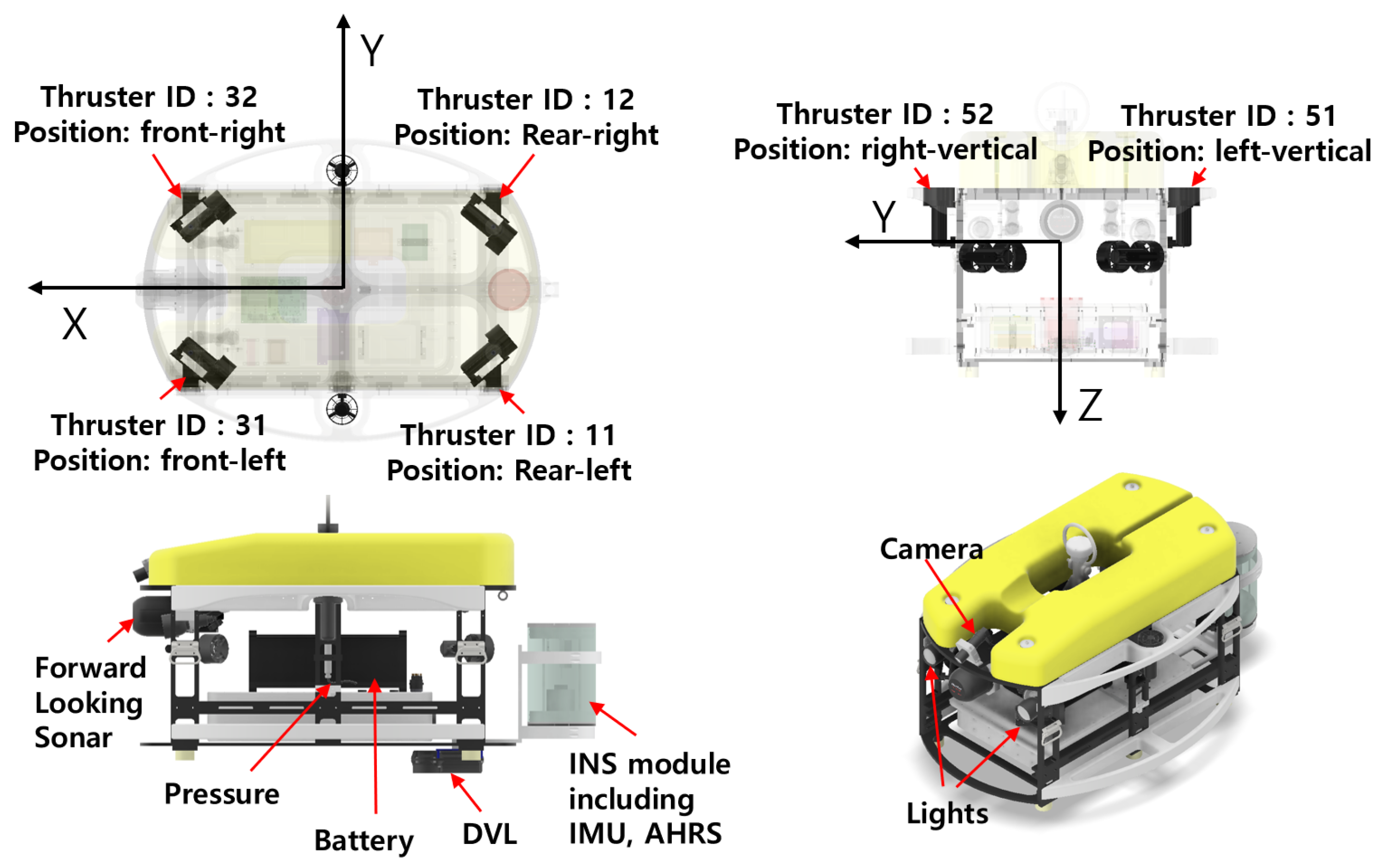
The P-SUROII is a test platform developed for the implementation and verification of core technologies such as control and navigation algorithms, and its external structure is shown in Figure 1. It is a hybrid unmanned underwater vehicle (UUV) capable of operating selectively in both AUV and ROV modes. The vehicle features a box-type frame that supports a high payload. Equipped with four horizontal thrusters and two vertical thrusters, it is capable of four DoF motion, including surge, sway, heave, and yaw. To enable navigation functionality, an inertial navigation system (INS) module is installed, which includes GPS, pressure sensor, inertial measurement unit (IMU), doppler velocity log (DVL), and attitude heading reference system (AHRS). Additionally, a forward-looking sonar (FLS), camera, and two lights are mounted on the vehicle [20]. The detailed sensor configuration and specifications can be found in Figure 2 and Table 1, respectively. In this study, the P-SUROII is operated in AUV mode to minimize the external forces acting on the vehicle. For the purpose of minimal state observation and control, only an optical tether cable with a diameter of 0.002m is used. Considering the maximum speed of the P-SUROII and the conditions of the test tank environment, the drag force is considered negligible.

2.1.2. Vehicle Kinematics and Dynamics

The six DoF nonlinear equations of motion governing the vehicle kinematics and dynamics can be expressed as follows [21]:
η ˙ = J ( η ) ν ,
M ν ˙ + C ( ν ) ν + D ( ν ) ν + g ( η ) = τ ,
where M = M a + M rb , with M a R 6 × 6 and M rb R 6 × 6 , denotes the total inertia matrix composed of the added mass and rigid-body inertia matrices, respectively. Similarly, C = C a + C rb , with C a R 6 × 6 and C rb R 6 × 6 , represents the combined Coriolis and centripetal matrices due to the added mass and rigid-body effects, respectively. In addition, D ( ν ) R 6 × 6 is the hydrodynamic damping matrix, and g ( η ) R 6 denotes the restoring force and moment vector resulting from the gravity and buoyancy. τ R 6 is the generalized control input vector consisting of the forces and moments acting on the underwater vehicle. Finally, J ( η ) is a nonlinear transformation matrix that maps vectors from the body-fixed frame to the navigation frame, and it varies with the vehicle’s position and orientation vector η = [ x y z ϕ θ ψ ] . It is defined as follows:
J ( [ ϕ θ ψ ] ) = J 1 ( η ) 0 3 × 3 0 3 × 3 J 2 ( η ) ,
where J 1 ( [ ϕ θ ψ ] ) is the transformation matrix that converts the linear velocity expressed in the body-fixed frame to the corresponding velocity in the navigation frame, while J 2 ( [ ϕ θ ψ ] ) transforms the angular velocity in the body-fixed frame into the rate of change of Euler angles in the navigation frame. These matrices are explicitly given by
J 1 ( [ ϕ θ ψ ] ) = c ψ c θ s ψ c ϕ + c ψ s θ s ϕ s ψ s ϕ + c ψ s θ c ϕ s ψ c θ c ψ c ϕ + s ψ s θ s ϕ c ψ s ϕ + s ψ s θ c ϕ s θ c θ s ϕ c θ c ϕ ,
J 2 ( [ ϕ θ ψ ] ) = 1 s ϕ t θ c ϕ t θ 0 c ϕ s ϕ 0 s ϕ / c θ c ϕ / c θ ,
with s ( · ) = sin ( · ) , c ( · ) = cos ( · ) , t ( · ) = tan ( · ) .
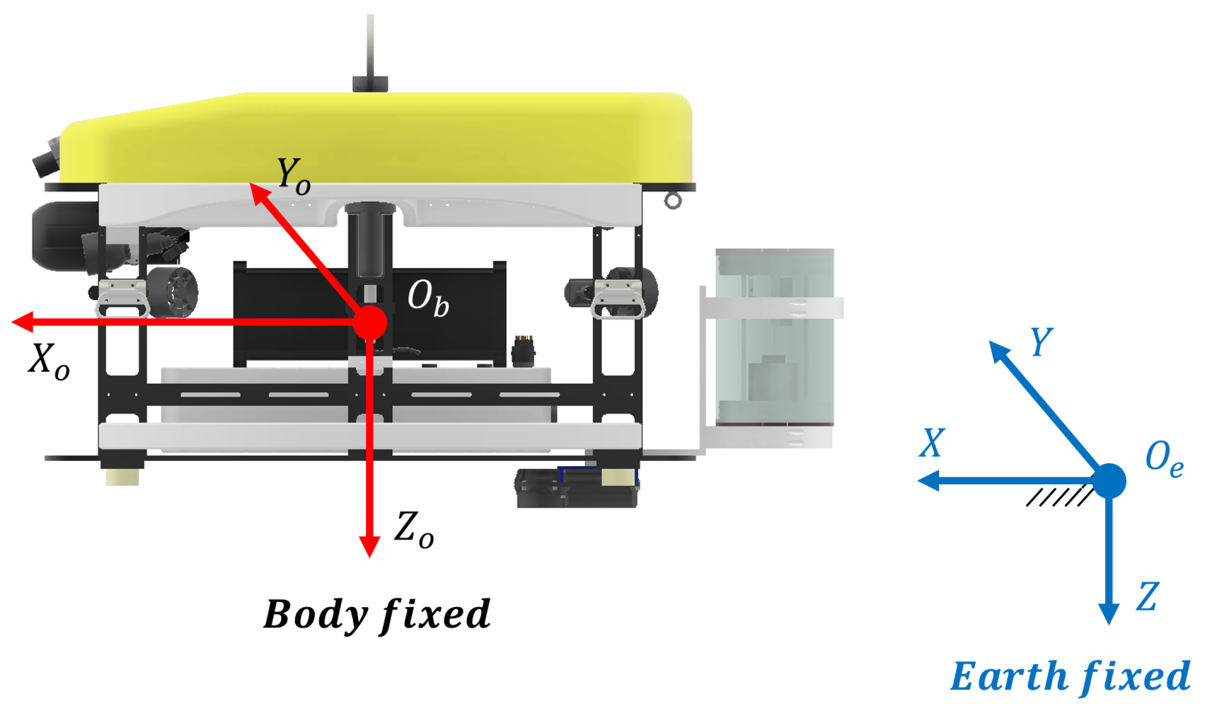
The coordinate systems adopted in this study are defined as the body-fixed frame O b and the navigation frame O e , as illustrated in Figure 3.

2.1.3. Derivation of Nonlinear Dynamics

In this paper, Equation (2), which exhibits strong nonlinearity and coupling, is simplified by deriving the equations based on the following assumptions [16,19,21], thereby reducing the number of coefficients to be estimated in the subsequent least squares method (LSM) and improving the accuracy of the parameter estimation.
  • P-SUROII is a low-speed UUV.
  • P-SUROII has three planes of symmetry.
  • The center of buoyancy of P-SUROII coincides with the body-fixed coordinate O b .
  • The center of gravity is assumed to be at (0, 0, z g ), where z g is a non-zero value.
With these assumptions, the vehicle’s rigid-body dynamics are given as follows [19]:
M a = diag X u ˙ , Y v ˙ , Z w ˙ , K p ˙ , M q ˙ , N r ˙ ,
M r b = m 0 0 0 m z g 0 0 m 0 m z g 0 0 0 0 m 0 0 0 0 m z g 0 I x x 0 0 m z g 0 0 0 I y y 0 0 0 0 0 0 I z z ,
C a ( ν ) = 0 0 0 0 Z w ˙ w 0 0 0 0 Z w ˙ w 0 X u ˙ u 0 0 0 Y v ˙ v X u ˙ u 0 0 Z w ˙ w Y v ˙ v 0 N r ˙ r M q ˙ q Z w ˙ w 0 X u ˙ u N r ˙ r 0 K p ˙ p Y v ˙ v X u ˙ u 0 M q ˙ q K p ˙ p 0 ,
C r b ( ν ) = 0 0 0 0 m w 0 0 0 0 m w 0 0 0 0 0 m v m u 0 0 m w m v 0 I z z r I y y q m w 0 m u I z z r 0 I x x p m v m u 0 I y y q I x x p 0 ,
D = diag X u , Y v , Z w , K p , M q , N r + diag X u | u | | u | , Y v | v | | v | , Z w | w | | w | , K p | p | | p | , M q | q | | q | , N r | r | | r | ,
g ( η ) = ( W B ) sin θ ( W B ) cos θ sin ϕ ( W B ) cos θ cos ϕ z g W cos θ sin ϕ z g W sin θ 0 ,
where X u ˙ , Y v ˙ , Z w ˙ , K p ˙ , M q ˙ , and N r ˙ denote the added mass coefficients along the corresponding axes. I x x , I x x , and I z z are the inertia moments, m is the mass, and z g is the position of the center of gravity along the z-axis. W and B represent the vehicle’s weight and buoyant force, respectively. Based on the aforementioned assumptions, P-SUROII is a low-speed UUV with three planes of symmetry. Therefore, the diagonal elements of the matrix in Equation (6) are sufficiently small to be neglected, and the higher-order terms in Equation (10) can also be omitted.
Based on the definitions above, the resulting four DoF equation can be derived as follows:
τ X = u ( X u + X u | u | | u | ) sin θ ( B W ) + q ( Z w ˙ w + m w ) + u ˙ ( X u ˙ + m ) + m q ˙ z g , τ Y = v ( Y v + Y v | v | | v | ) p ( Z w ˙ w + m w ) + v ˙ ( Y v ˙ + m ) + cos θ sin ϕ ( B W ) X u ˙ r u m p ˙ z g , τ Z = w ( Z w + Z w | w | | w | ) + m w + q ( X u ˙ u m u ) p ( Y v ˙ v m v ) + w ˙ ( Z w ˙ + m ) + cos ϕ cos θ ( B W ) , τ R = r ( N r + N r | r | | r | ) q ( I x x p K p ˙ p ) + p ( I y y q M q ˙ q ) + v ( X u ˙ u m u ) u ( Y v ˙ v m v ) + r ˙ ( I z z + N r ˙ ) ,
where the motion in the ϕ and θ directions is considered to be passively stable for P-SUROII, and thus, the corresponding dynamic equations are omitted.

2.2. Thruster Model

As previously mentioned, the P-SUROII is equipped with a total of six thrusters, of which four are mounted in the horizontal direction and two in the vertical direction. To estimate the hydrodynamic coefficients based on the proposed dynamic model (12), it is necessary to know the direction and magnitude of the thruster forces acting on the UUV. However, since an accurate model of the thrusters is not provided, the exact thrust magnitude cannot be determined. In this study, a bollard pull test is conducted to estimate the thruster model. The maximum thrust of the thruster is approximately 60 N, and the maximum usable rotational speed is ± 4500  RPM. Nevertheless, to ensure the safety of the thrusters, the operating RPM range in the experiment is limited to ± 3400  RPM.
Although several studies, including [22], have proposed high-fidelity thruster models, the complexity of these models and the difficulty of conducting experiments to estimate their coefficients do not align with the objectives of this study. Therefore, the simplified thruster model employed in this study can be expressed as follows:
T i = T | n | n · | n | n + T | n | v a · | n | v a , v a = ( 1 w ) · v ,
where T i denotes the thrust output of the i-th thruster, while T n | n and T n | v a represent the thruster coefficients under static and dynamic flow conditions, respectively. n is the input RPM of the thruster, v a is the advance speed, w is the wake fraction coefficient, and v denotes the vehicle’s velocity. Considering the characteristics of the bollard pull test and the fact that P-SUROII operates as a low speed with a maximum speed of 0.5 m/s, the advance speed is assumed to be negligible, i.e., v a 0 . To better fit the thrust response curve, a simplified quadratic thruster model is adopted in this study, as given below:
T i = T | n | n · | n | n + T | n | · n .
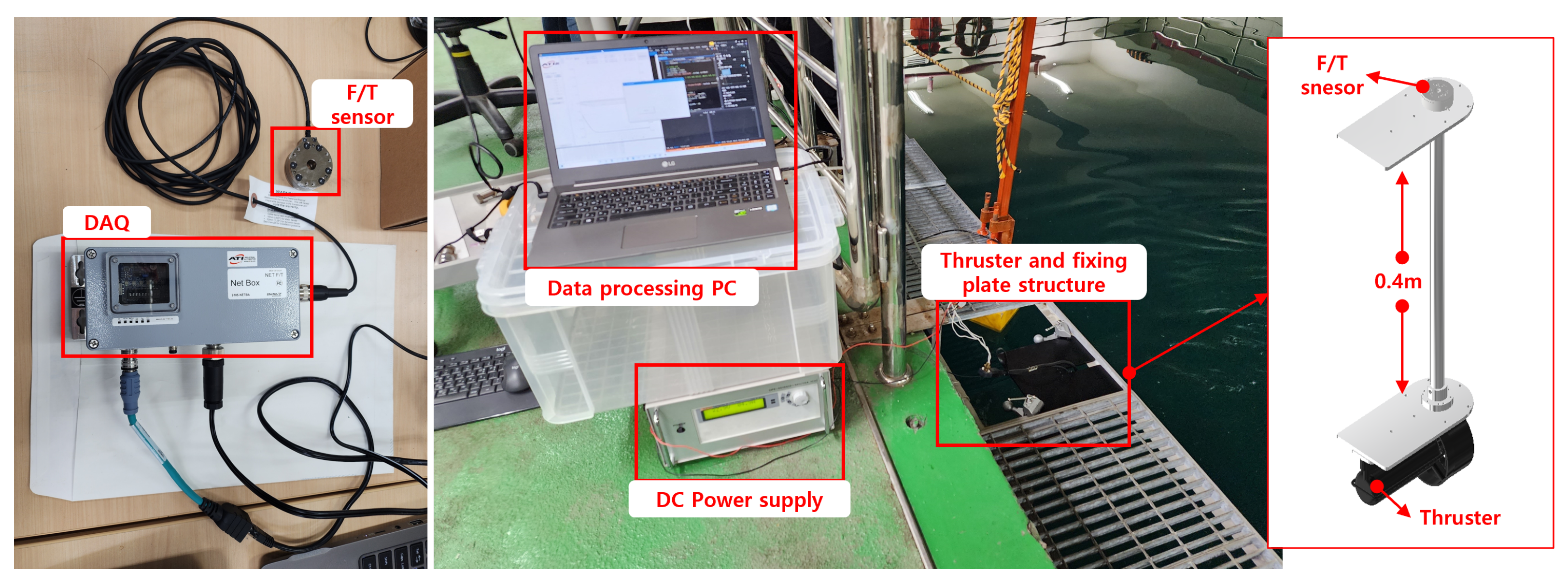
To estimate T | n | n and T | n | for each thruster, the thruster was mounted on a fixed structure equipped with a six-axis force/torque sensor. The thruster was operated with continuous inputs ranging ±3400 RPM in 100 RPM increments, and the forces and moments were measured. The experimental setup and configuration are shown in Figure 4. The force generated by the thruster was measured by the F/T sensor, and the sensor data were transmitted to the PC via the DAQ system. Experiments were conducted on the four horizontal thrusters. The vertical thrusters were excluded from testing, as they are only responsible for the vertical motion, and the roll motion of the P-SUROII is inherently stable.
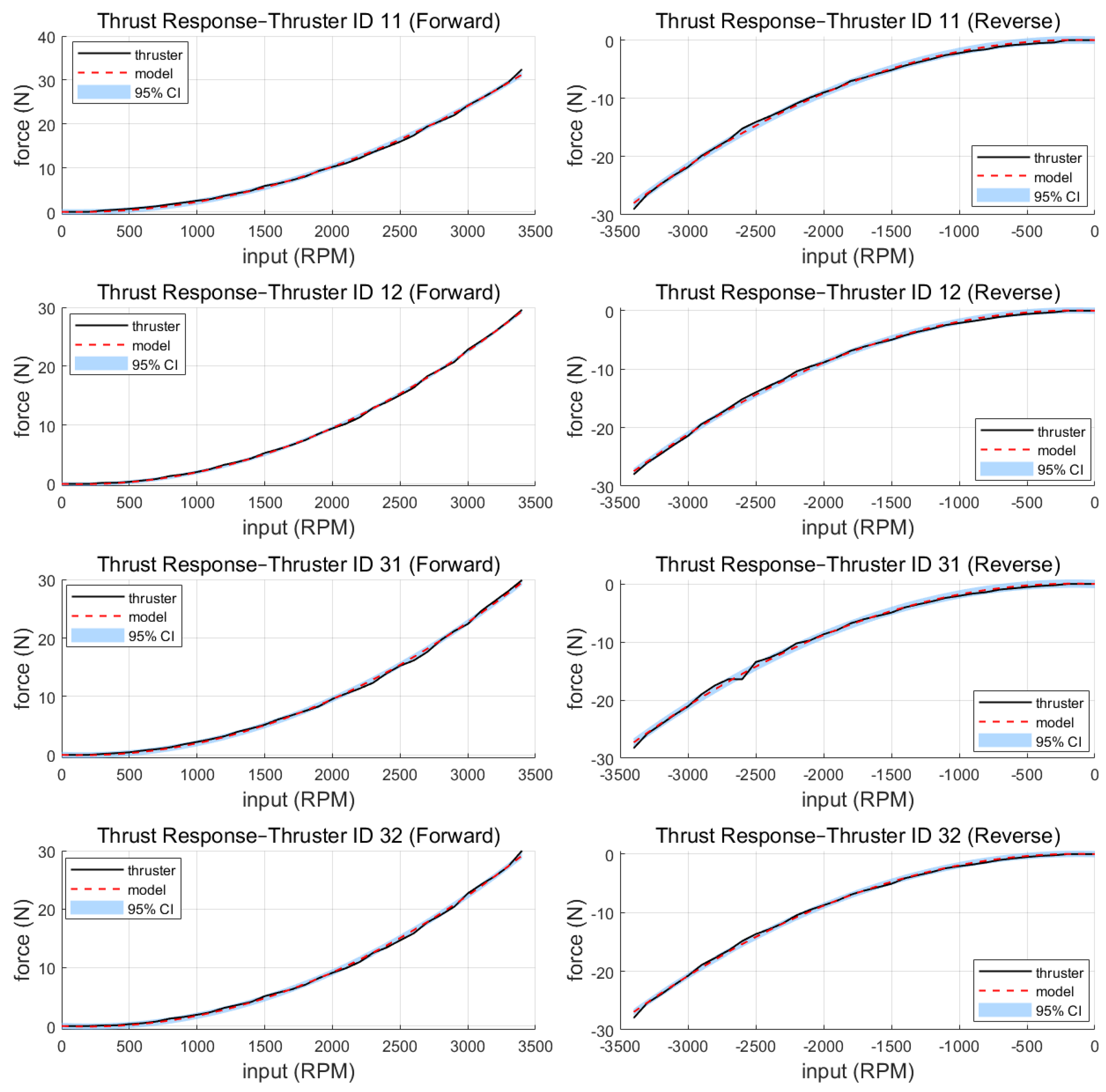
Each thruster exhibited a dead zone in the range of approximately ±300 RPM on average. The thrust measured by the F/T sensor and the corresponding RPM input data were used to estimate the coefficients of a second-order polynomial model using the LSE method. To account for the difference in thrust characteristics between the forward and reverse directions, the coefficients were estimated separately for each direction. The resulting thrust curve and corresponding model coefficients are presented in Figure 5 and Table 2, respectively. The solid black line represents the experimentally measured thrust, while the red dashed line indicates the thrust estimated using the model. The shaded regions correspond to the 95% confidence intervals (CI) derived from the residual errors. A comparison between the estimated and measured thrust shows that the differences remain within an acceptable range at the 95% confidence level, confirming the reliability of the model.

2.3. Motion Sensor

In general, due to physical constraints, it is not feasible to align the central axes of individual sensors with the center of an underwater vehicle. As a result, each sensor is installed at an offset from the vehicle’s center, which introduces measurement errors in the sensor data. To address this, the position and orientation offsets of each sensor must be properly compensated, so that the measurements can be accurately utilized as motion data for the UUV [23,24].

2.3.1. IMU Measurement Correction

The IMU is installed on the UUV at a position ( X I M U , Y I M U , Z I M U ) and orientation ( ϕ I M U , θ I M U , ψ I M U ) ) with respect to the body-fixed coordinate, and the angular rate ω b can be expressed as follows [24].
ω b = J 1 ( ϕ I M U , θ I M U , ψ I M U ) · ω imu b ,
where ω imu b represents the angular rate measured by the IMU.
The acceleration V I , derived from the center point velocity V I of the IMU, can be expressed as follows [24].
f b = V ˙ imu ω ˙ b × L imu ω b × V b ω b × ( ω b × L imu ) ,
where V ˙ imu denotes the acceleration measured by the IMU, ω ˙ b is the angular acceleration, L imu is the IMU installation position with respect to the center point of IMU, and V b is the compensated DVL velocity [24]. The angular acceleration is estimated using a low-pass filter, as expressed in the following equation.
ω ˙ m ( t ) = ω imu b ( t ) ω imu b ( t 1 ) / Δ t , ω ˙ b ( t ) = ( 1 α ) · ω ˙ ( t 1 ) + α · ω ˙ m ( t ) ,
where Δ t represents the sampling time, and α is the order parameter of the filter ( 0 < α < 1 ).

2.3.2. DVL Measurement Correction

The DVL is installed on the UUV at a position ( X D V L , Y D V L , Z D V L ) and orientation ( ϕ D V L , θ D V L , ψ D V L ) with respect to the body-fixed coordinate, and the compensated volocity of the DVL V b can be expressed as follows [24].
V b = J 1 ( [ ϕ dvl , θ dvl , ψ dvl ] ) · V dvl b ω b × L dvl ,
where V dvl b donates the velocity measured by the DVL, and L dvl is the installation position of the DVL with respect to the center point of the DVL [24].

3. Methodology

This section describes an overview of the SI procedure applied to the P-SUROII. The implementation of the CRLS method adopted in this study is described in detail, and its validity is verified through simulation. In addition, the dataset used for SI and validation is explained in detail, and the identified hydrodynamic coefficients as well as the results of the control simulations based on these coefficients are presented and analyzed.

3.1. SI Methods

3.1.1. Related Works

As previously mentioned, SI refers to the process of estimating a mathematical model of a target system based on actual experimental data. The most representative method, LSE, is mathematically simple and computationally stable. However, it is unsuitable for real-time estimation and is sensitive to noise and bias, making it prone to accumulated estimation errors. The RLSE improves upon this by updating parameters in real time based on previous estimates. Nevertheless, it may suffer from reduced stability due to the potential divergence of the covariance matrix and remains vulnerable to noise and bias. The RPEM updates parameters by computing the total derivative of the prediction error between the model output and the actual output. This approach is applicable to nonlinear systems and offers some robustness to noise. However, it has the drawback of misinterpreting bias as a system characteristic, thereby distorting the parameter estimation. The IVM mitigates the noise correlation between input and output by introducing instrumental variables, offering strong robustness to both noise and bias. Still, it imposes strict conditions for selecting valid instruments, limiting its practical applicability. To overcome the limitations of these existing methods, this study employs the CRLS algorithm. The CRLS extends the RLS framework by incorporating linear equality or inequality constraints, allowing predefined or adjustable bounds on the estimated parameters. This helps suppress excessive estimation deviation and enables high-precision parameter identification, even in environments with noise and bias. However, as the complexity of the constraints increases, the computational burden grows, and the estimation results may become highly sensitive to the configuration of the constraints. To mitigate this, the CFD was used to define the initial constraint boundaries, thereby enhancing the stability of the constraint settings.
In terms of the previous studies, the study in [13] applied the least squares method to estimate the parameters from experimental data and verified the statistical validity of the results by presenting the uncertainty of the estimated values in terms of CI. For nonlinear problems, the Gauss–Newton method, the Marquardt algorithm, and the Nelder–Mead method were employed to improve the convergence and robustness, thereby significantly enhancing the applicability of the parameter estimation in the real experimental data analysis. The study in [14] proposed an LSE-based parameter identification method for estimating the hydrodynamic coefficients of AUVs in the presence of measurement biases, where a Complementary Kalman Filter (CKF) was used to compensate for the measurement bias, and the LSE was then applied to obtain unbiased coefficients. The study in [16] introduced an online system identification technique, in which the CRLS was applied to a custom-built underwater robotic platform to estimate the dynamic model in real time, and tank experiments demonstrated that safe and efficient parameter identification could be achieved online. In addition, the study in [17] proposed an adaptive estimation technique using the PREM approach, which incorporates unknown parameters into the state vector of linear state–space models and recursively minimizes prediction errors, thereby estimating both parameters and states simultaneously. The study in [18] addressed continuous time model identification based on sampled data, implemented and evaluated through the continuous time system identification (CONTSID) matlab toolbox, and performed sensitivity analyses under various noise conditions and input signals, along with comparisons to indirect methods. Finally, the study in [1] applied the IVM method to identify the heading-related dynamic coefficients of an underwater cable laying robot and utilized the identified parameters for heading controller design.

3.1.2. Proposed Method

In this study, the CRLS method was adopted to robustly estimate parameters from real underwater experimental data containing noise and bias. Furthermore, the initial constraint conditions were defined through CFD analysis, and constraint tuning was conducted during the identification process to enhance the estimation accuracy. To further improve the integration with the actual underwater robotic system, acceleration information was estimated based on an SDINS and the dynamic model and used for model validation.
Algorithm 1 shows the CRLS algorithm procedure for Hydrodynamic Parameter Estimation. First, the sensor raw measurements obtained through experiments are corrected. Then, the covariance matrix P ( t ) , which represents the uncertainty of the parameter estimation, is computed. Based on this, the prediction error e ( t ) , defined as the difference between the actual output and the predicted output using the currently estimated parameters, is calculated. The Kalman gain K ( t ) , which serves as a weighting factor for the estimation update, is then computed. The estimated parameters θ ^ ( t ) consist of the first- and second-order damping coefficients and the added mass for each axis. These parameters are constrained within the bounds θ min and θ max , which are determined based on the criteria described below.
  • The damping and added mass values are assumed to be greater than zero ( θ ^ ( t ) > 0).
  • The initial values of the damping coefficients are set to the damping coefficients obtained from the CFD analysis.
  • Since the P-SUROII is a larger system than the BlueROV2, the corresponding parameter values are set to be higher than those of the BlueROV2.
  • The minimum and maximum bounds of each parameter are iteratively adjusted and optimized based on the experiments and simulation results.
Algorithm 1 CRLS algorithm for Hydrodynamic Parameter Estimation
 1:
Input:  ϕ , θ , ψ , u , v , w , p , q , r , u ˙ , v ˙ , w ˙ , p ˙ , q ˙ , r ˙
% P-SUROII motion data
 2:
Output:  X u , X u | u | , Y v , Y v | v | , Z w , Z w | w | , N r , N r | r | , X u ˙ , Y v ˙ , Z w ˙ , N r ˙
% Hydrodynamic coefficients and added mass terms
 3:
for  t = 1 to n do
 4:
    Obtain sensor raw measurement: P-SUROII motion data
 5:
    Measurement correction
 6:
    % Calculation of the CRLS algorithm
 7:
     P ( t + 1 ) = P ( t ) K ( t ) X T ( t + 1 ) P ( t )
 8:
     e ( t + 1 ) = y ( t + 1 ) X T ( t + 1 ) θ ^ ( t )
 9:
     K ( t + 1 ) = P ( t ) X ( t + 1 ) 1 × 10 9 + X T ( t + 1 ) P ( t ) X ( t + 1 ) + R
10:
     θ ^ ( t + 1 ) = θ ^ ( t ) + K ( t + 1 ) e ( t + 1 )
11:
     θ ^ ( t + 1 ) = m a x ( θ min , m i n ( θ ^ ( t + 1 ) , θ max ) )
12:
end for
13:
return  θ ^ ( t )
In general, constraints on parameter estimates can be imposed based on several considerations, including physical feasibility, empirical observations, and system stability. In this study, a hybrid constraint strategy is adopted, combining physically meaningful bounds—derived from the inherent limitations of the parameters (e.g., positive mass or drag coefficients)—and empirical bounds obtained from experimental and operational data. Specifically, the lower and upper bounds for each parameter are defined using a combination of physical interpretation and empirical evidence. These bounds are then applied as hard constraints in the CRLS update step and iteratively tuned through repeated estimation to ensure the consistency and physical relevance of the estimated parameters.

3.2. Simulation Studies

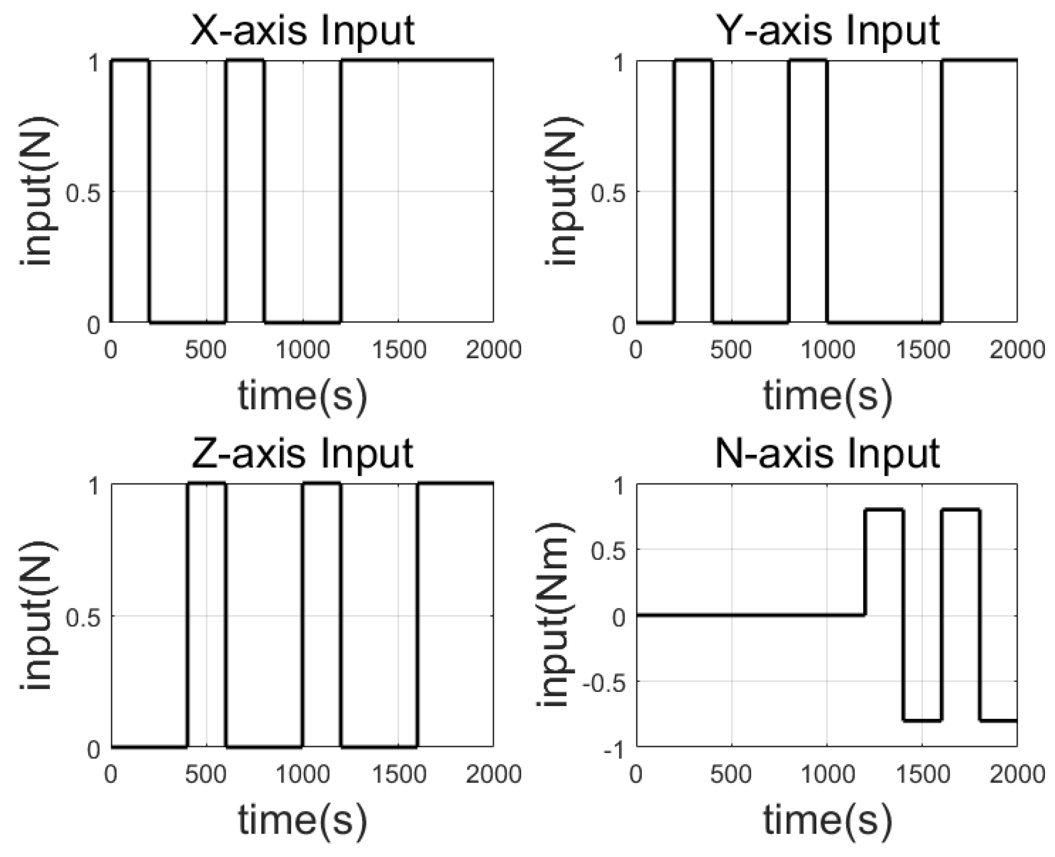
In this study, the CRLS algorithm is employed to estimate the hydrodynamic coefficients of the P-SUROII. Prior to applying the method to actual data, a simulation was conducted using the BlueROV2 model [19] to verify the correctness of the CRLS equations and the associated MATLAB (24.2.0.2712019 (R2024b)) implementation. To generate the data for the identification process, a low frequency input signal was applied to the predefined BlueROV2 model, which represents the dynamics of an underwater vehicle. The estimated hydrodynamic coefficients obtained via the CRLS were then compared against the ground truth values used in the simulation model to validate the numerical stability and correctness of the CRLS formulation. Notably, UUVs are characterized by high inertia and significant hydrodynamic damping, which results in sluggish responses to rapidly varying inputs. Consequently, high-frequency input components may not be physically transmitted to the vehicle or may be suppressed as noise. In addition, a certain level of noise and bias was added to the acquired acceleration data to simulate the system under conditions as close as possible to the real-world environment. Since UUVs are generally assumed to be stable in roll and pitch, control inputs were applied over time only in the surge, sway, heave, and yaw directions, as shown in Figure 6, both in decoupled and coupled forms, to induce motion in all degrees of freedom.
The simulation, as described in Algorithm 2, involved generating a dataset by applying predefined noise and bias to motion data obtained from the BlueROV2 dynamic model. The accuracy of parameter estimation was then evaluated using the CRLS algorithm.
Algorithm 2 Synthetic data generation and CRLS-based parameter estimation for BlueROV2
     Parameters:  X u , X u | u | , Y v , Y v | v | , Z w , Z w | w | , K p , K p | p | , M q , M q | q | , N r , N r | r | , X u ˙ , Y v ˙ , Z w ˙ , K p ˙ , M q ˙ , N r ˙
 2: % Hydrodynamic coefficients and added mass terms
 
     % Step 1: Data Generation from the Dynamic Model
 4: for i = 1 to n do
          Generate control input U ( i )
 6:      Simulate motion using BlueROV2 model: X d temp ( i )
          Add noise and bias: X d ( i ) = X d temp ( i ) + η ( i ) % η ( i ) : noise and bias
 8: end for
 
     % Step 2: Constrained Recursive Least Squares Estimation
10: for i = 1 to n do
          Define input–output structure of the dynamic system
12:     Perform CRLS estimation with physical constraints
          Store or validate estimated parameters
14: end for
As shown in Table 3, the hydrodynamic coefficients estimated using the CRLS algorithm are generally in close agreement with the reference values, with relatively small errors across most terms. In particular, key coefficients such as X u , Y v , K p , and M q were estimated with high accuracy. Although the largest deviation occurred in Z w w , the error remained within an acceptable range from a physical modeling perspective. These results demonstrate that the CRLS algorithm operated properly under the given simulation setup and can serve as a reliable tool for identifying the hydrodynamic parameters of underwater vehicles.

3.3. Experimental Studies

3.3.1. Data Acquisition

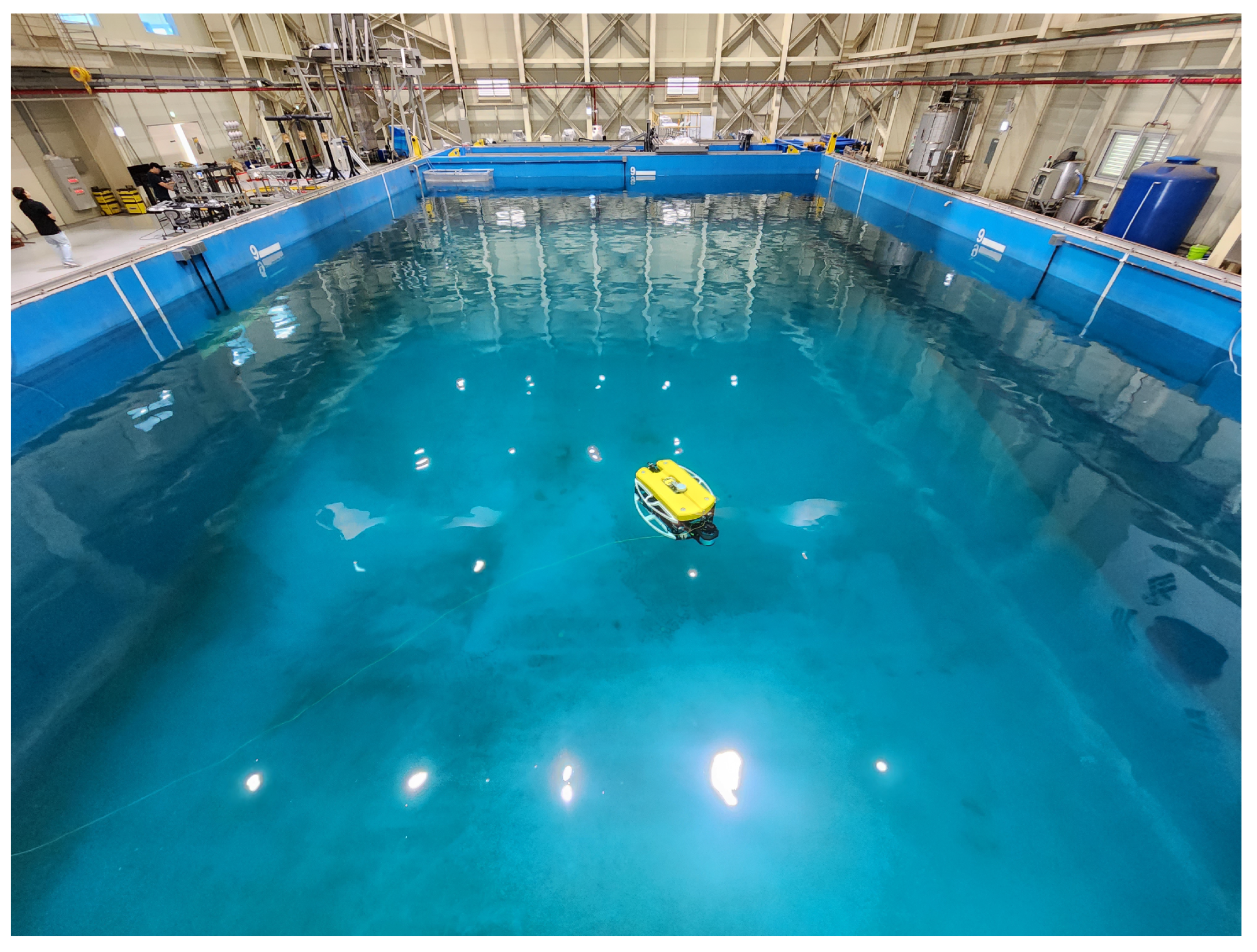
To acquire motion data of the P-SUROII, tests were conducted in a water tank with dimensions of 35 m in length, 20 m in width, and 9.6 m in depth, providing a disturbance-free environment and sufficient space for maneuvers, as shown in Figure 7. To minimize the influence of self-induced external forces and to ensure convenience during testing, the vehicle was operated in AUV mode using onboard batteries, with only a 0.002 m-thick optical communication cable connected.
In this study, experimental data were acquired and categorized according for two distinct purposes: parameter estimation and model validation. The dataset for estimation was designed to sufficiently activate the major hydrodynamic coefficients corresponding to the surge, sway, heave, and yaw directions, with sufficient distance and duration secured to include both acceleration and deceleration phases. For surge motion, eight datasets were obtained by varying the RPMs of the thrusters to induce forward motion. Likewise, eight datasets were collected for sway motion by actuating the thrusters in the starboard direction at different RPMs. One dataset was acquired for the heave motion by reversing the thrust direction of the vertical thrusters to generate vertical movement. For the yaw motion, 16 and 18 datasets were obtained in the clockwise and counterclockwise directions, respectively, by adjusting the RPM balance between the port and starboard thrusters to induce rotational motion. Among these, datasets with clearly distinguishable motion and high data quality were selected specifically, seven for surge, seven for sway, one for heave, and six for each yaw direction. These were combined into a single unified dataset in which the hydrodynamic forces in all directions were properly activated across RPM ranges, with the aim of enhancing the accuracy of parameter estimation. To validate the generalization capability of the model and the accuracy of the estimated parameters, separate tests were conducted: free-running trials and S-shaped maneuvers. The free-running test was designed to include a balanced combination of translational and rotational motions within a single dataset, while the S-shaped maneuver was intended to induce complex scenarios involving various motion components, allowing for comprehensive evaluation of the model’s predictive performance.

3.3.2. SI Result and Verification

Parameter identification for the P-SUROII was performed based on the experimental datasets and the CRLS algorithm, which was validated through simulation. The minimum and maximum values for imposing constraints on the parameters were initially set and then iteratively tuned through simulation.
The main physical parameters of the P-SUROII used in this study are summarized as Table 4.
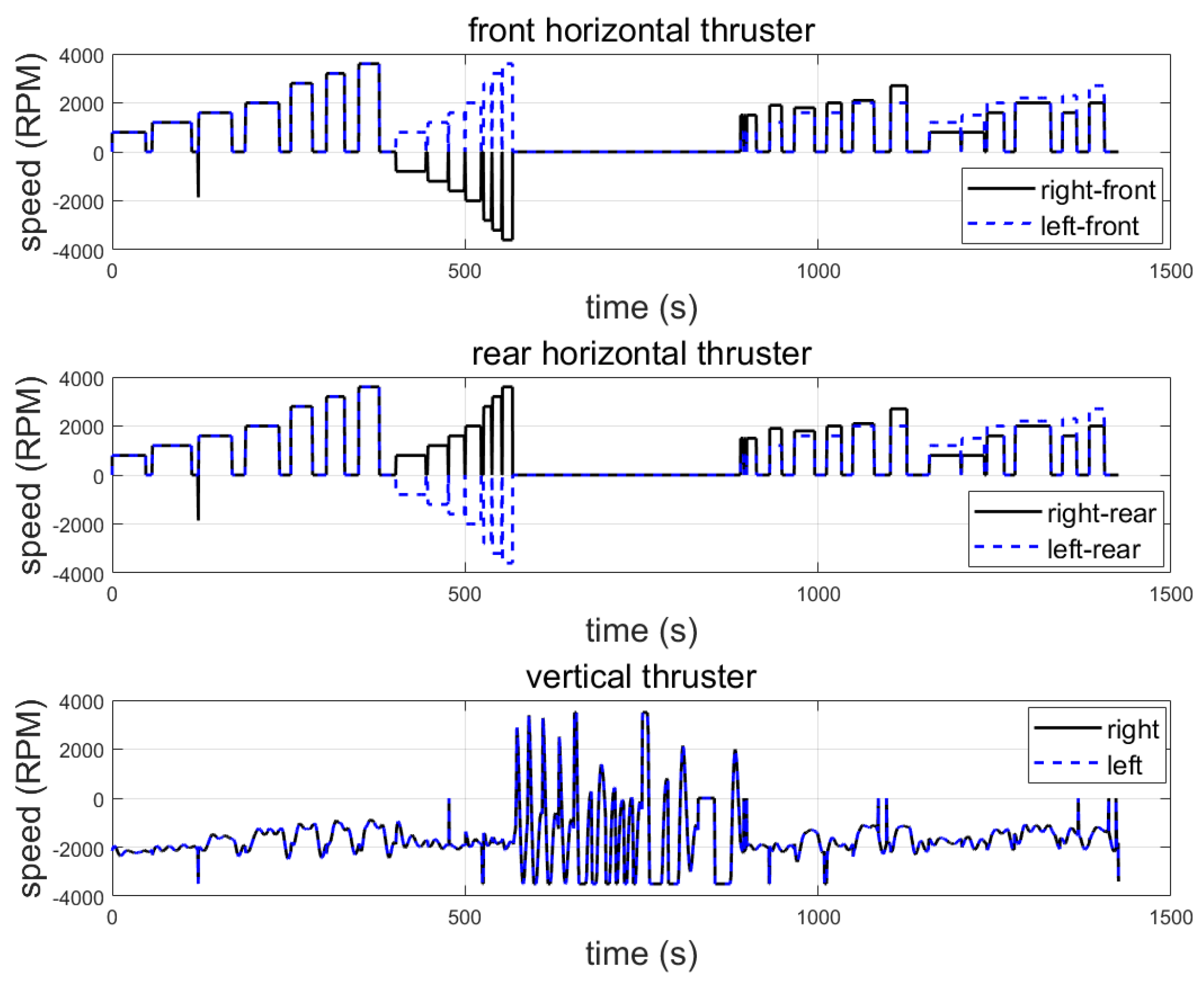
The hydrodynamic coefficients were first estimated using the unified dataset, and the thruster control inputs used in this dataset are presented in Figure 8. Each graph, in order, represents the control inputs of the forward port and starboard thrusters in the horizontal plane, the aft port and starboard thrusters in the horizontal plane, and the port and starboard thrusters in the vertical plane. From 0 s to approximately 378 s, all horizontal-plane thrusters were driven in the forward direction to perform forward motion. From 378 s to around 574 s, the forward starboard thruster and the aft port thruster were driven in reverse to perform lateral motion. Subsequently, from 574 s to about 904 s, only the vertical thrusters were operated to perform up and down motion, and during the remaining period, the outputs of the port and starboard thrusters were adjusted to perform yaw rotation of the hull. During the experiment, except for the period when up and down motion was performed, the vertical thrusters were continuously driven at approximately 2000 RPM to maintain a depth of 2 m.
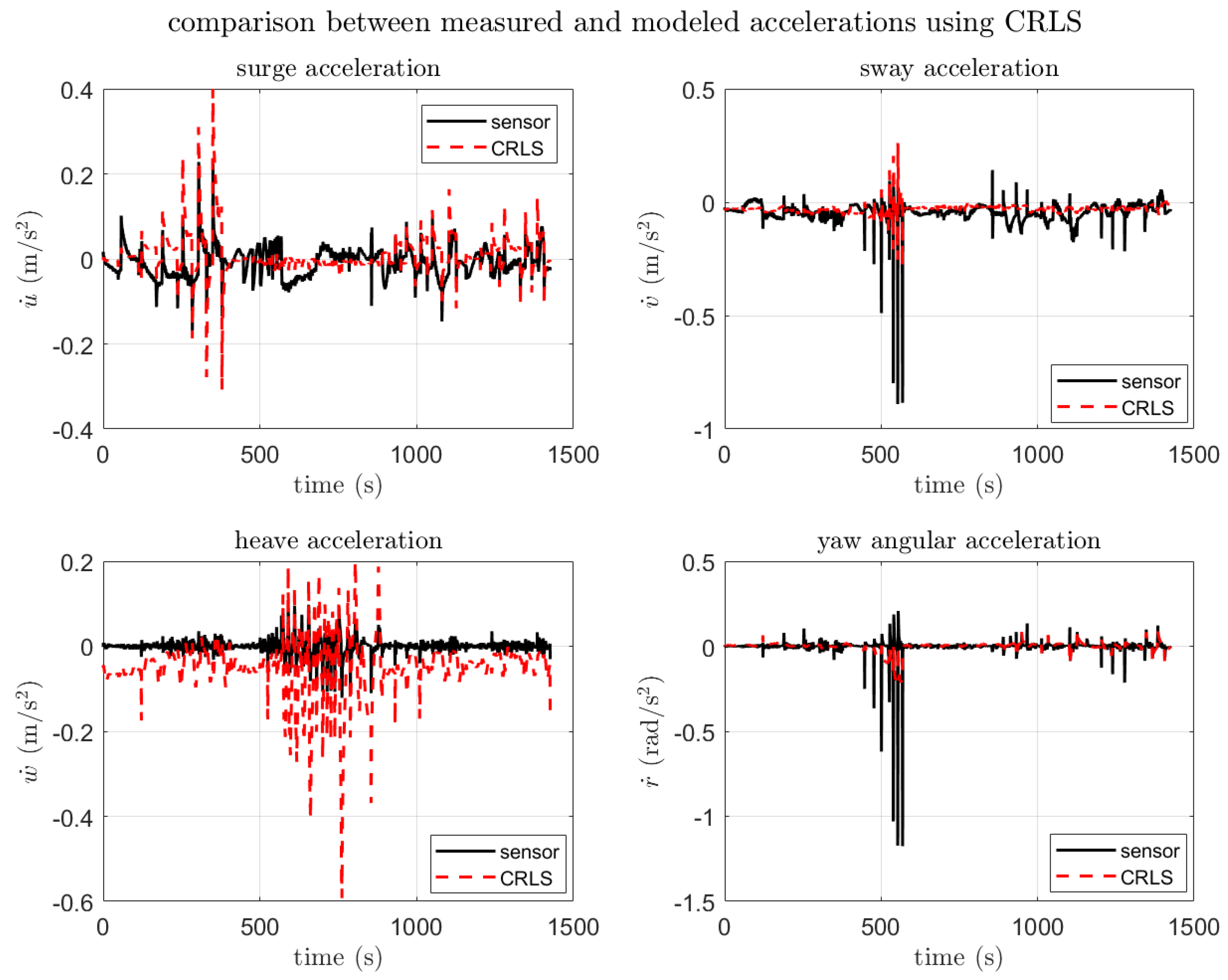
The estimated coefficients are presented in Table 5, and all values were identified as positive, consistent with the expected signs defined in the model formulation. To evaluate the validity of the identified parameters, the measured accelerations and angular accelerations from the unified dataset were compared with those computed from the P-SUROII model using the estimated coefficients, as shown in Figure 9. The measured acceleration data were processed using a moving average filter during graph generation to reduce signal noise and enhance readability for analysis.
The surge acceleration u ˙ varied approximately between 0.4 m / s 2 and 0.4 m / s 2 , and the CRLS model effectively captured the overall dynamic characteristics. The RMSE and MAE were 0.0465 and 0.0339, respectively, indicating a high level of estimation accuracy. However, some discrepancies were observed in segments involving vertical motion, likely due to the influence of the vertical thrusters.
The sway acceleration v ˙ was observed in the range of approximately 1.0 m / s 2 to 0.3 m / s 2 . The model successfully followed the overall trend, though it tended to underestimate short-duration peaks. The corresponding RMSE and MAE were 0.0470 and 0.0304, respectively, suggesting generally good performance. The heave acceleration w ˙ showed the largest variation, ranging from approximately 0.6 m / s 2 to 0.2 m / s 2 . In this axis, the model did not fully capture the high-frequency oscillations, resulting in the highest RMSE (0.0745) and MAE (0.0571) among all axes. This may be attributed to vertical disturbances or unmodeled dynamic coupling effects. The yaw angular acceleration r ˙ ranged from approximately 1.5 rad / s 2 to 0.5 rad / s 2 . The CRLS model reproduced the overall trend well, although some reduction in responsiveness was observed in segments with rapid directional changes. Nevertheless, with an RMSE of 0.0533 and MAE of 0.0250, the model demonstrated satisfactory estimation performance under steady-state and low-dynamic conditions. In summary, although some transient errors were observed, particularly in the heave direction, the CRLS-based model successfully reproduced the dynamic acceleration behavior of the underwater robot and demonstrated good accuracy and robustness across all degrees of freedom.
As mentioned earlier, this study employed two different types of motion data to verify the validity of the estimated coefficients. By comparing the results with those obtained using the RLS method, it was demonstrated that the parameters estimated through the CRLS approach achieved higher accuracy and reliability even in data environments contaminated with noise and bias.
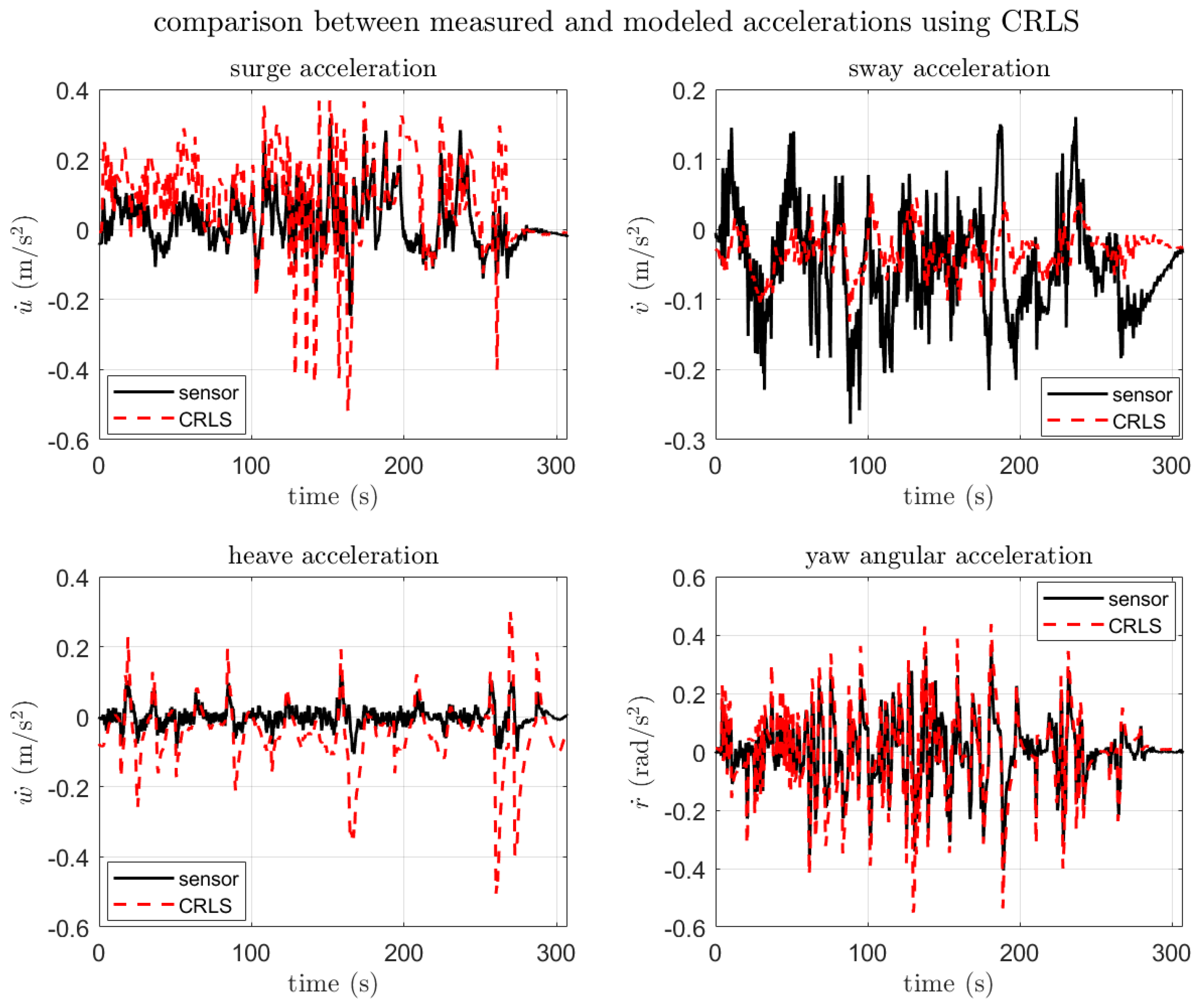
Figure 10 presents the motion data obtained from the free-running test. The surge acceleration u ˙ varied approximately between 0.6 m / s 2 and 0.4 m / s 2 , and the CRLS model successfully reproduced the overall trend. The RMSE and MAE for this axis were 0.1249 and 0.0910, respectively, indicating somewhat lower estimation accuracy compared to the previous experiment. The sway acceleration v ˙ was observed in the range of approximately 0.3 m / s 2 to 0.2 m / s 2 . The model effectively followed the low-frequency components but tended to underestimate the sharp peaks and rapid variations. As a result, the RMSE and MAE were 0.0780 and 0.0627, respectively. The heave acceleration w ˙ exhibited the largest variation, ranging from 0.6 m / s 2 to 0.4 m / s 2 . While the model accurately followed the measurements in steady-state segments, significant errors occurred during oscillatory motion. Consequently, the RMSE and MAE were 0.0926 and 0.0675, respectively, which were among the highest across all axes. The yaw angular acceleration r ˙ was observed within the range of approximately 0.5 rad / s 2 to 0.6 rad / s 2 . The model successfully captured the repeated oscillatory behavior but showed reduced responsiveness in rapid transitions and high-frequency rotational motion. The RMSE and MAE were 0.0795 and 0.0549, respectively, indicating a reasonable level of estimation performance for rotational dynamics. In summary, the CRLS model demonstrated good agreement with the measured accelerations overall but showed relatively reduced accuracy under free-running conditions, particularly in segments with fast transitions or high-frequency motions.
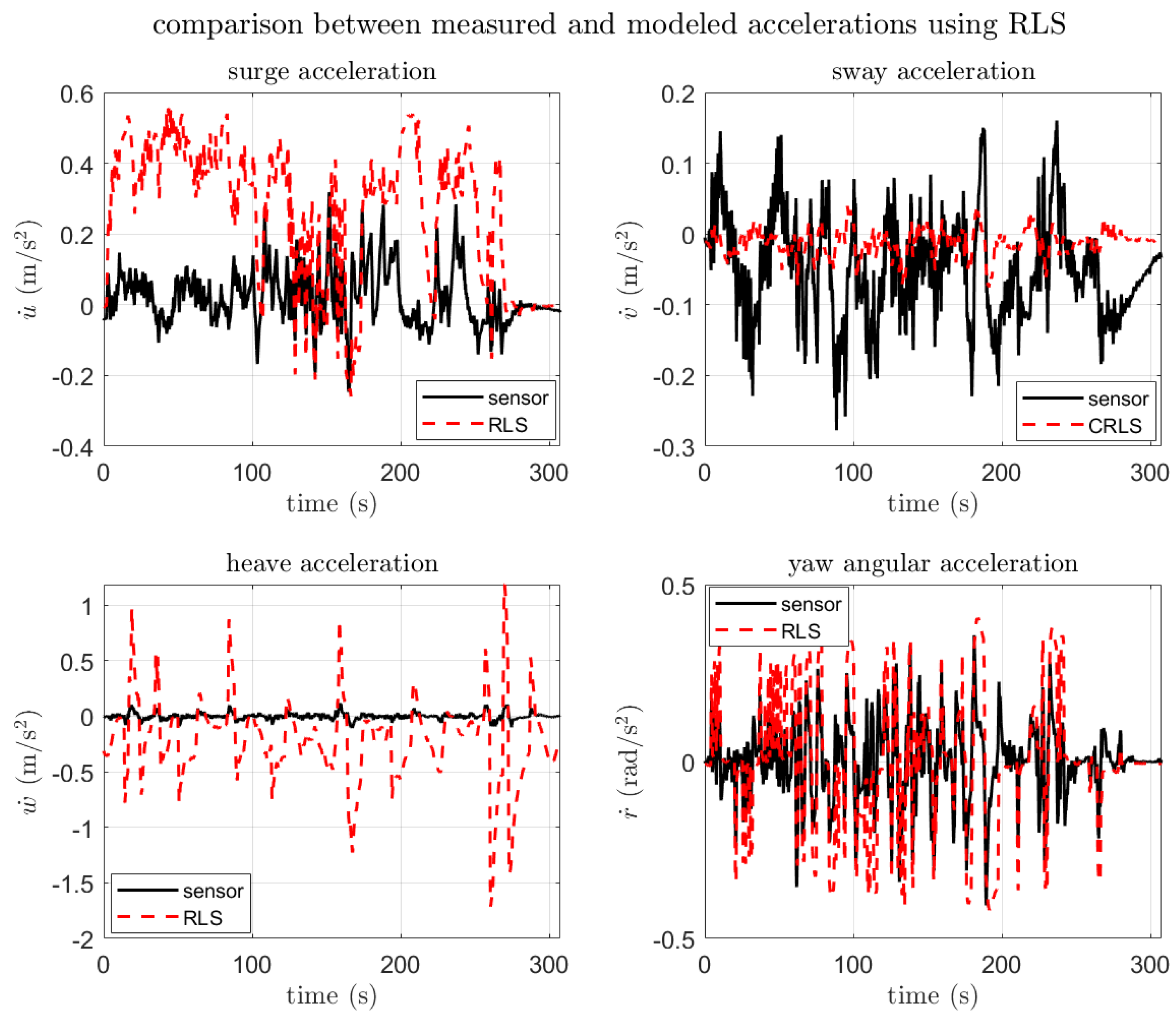
Figure 11 illustrates the comparison between the free-running motion data and the RLS-based model. While the RLS model generally follows the trend of the measured data, its accuracy significantly deteriorates under free-running conditions due to noise, bias, and rapid dynamic variations, clearly revealing its inferior performance compared to the CRLS-based approach.
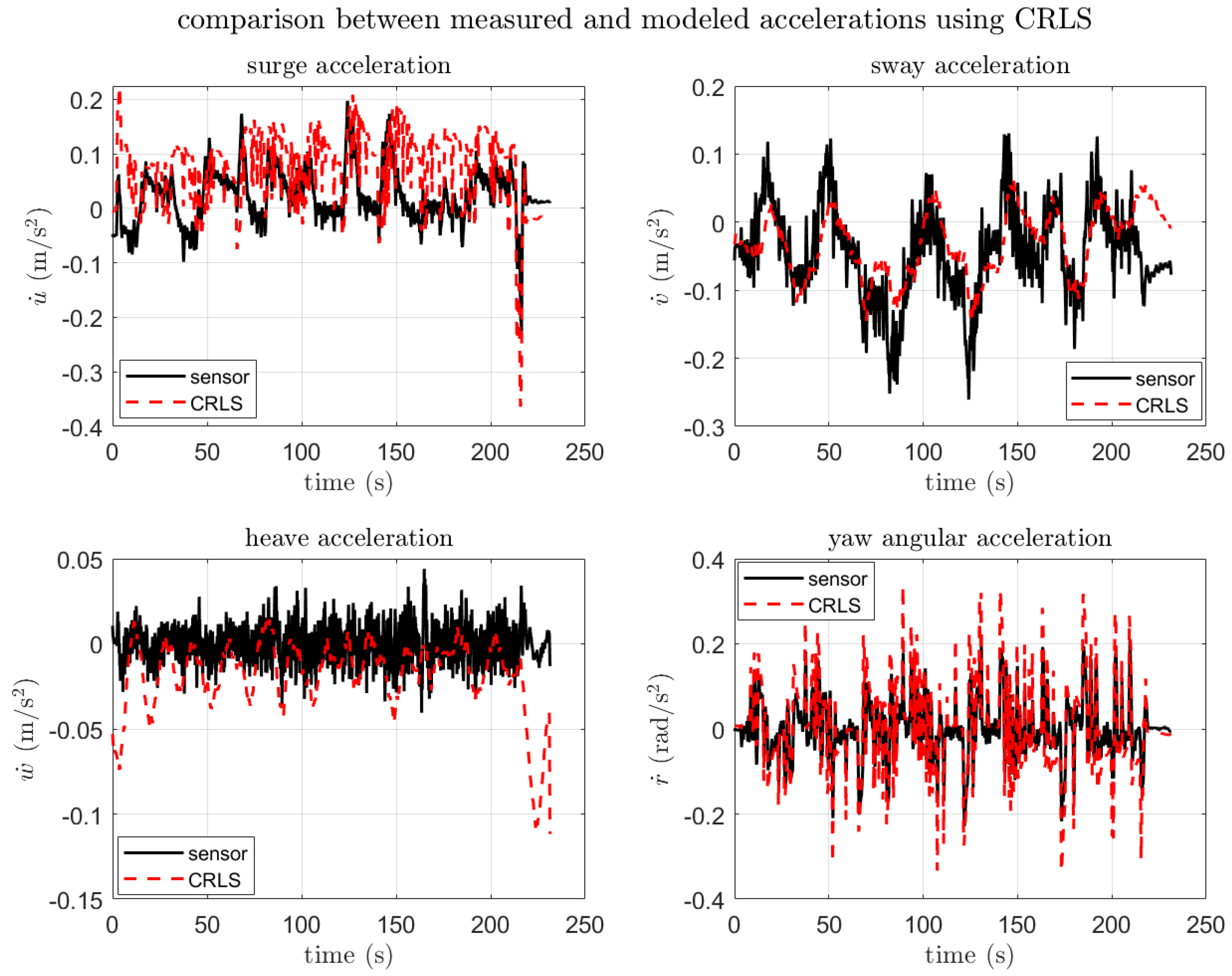
Figure 12 shows a comparison between the sensor-based acceleration and angular acceleration data obtained from the S-shaped maneuver experiment and the outputs of the CRLS-based model. The surge acceleration u ˙ varied approximately between 0.4 m / s 2 and 0.3 m / s 2 , and the CRLS model successfully followed the overall trend. However, in certain rising segments, the model exhibited overestimation compared to the measured data. The RMSE and MAE for this axis were 0.0994 and 0.0810, respectively, indicating a reasonable level of estimation accuracy. The sway acceleration v ˙ was observed in the range of approximately 0.3 m / s 2 to 0.2 m / s 2 . The model accurately reproduced the low-frequency variations, although the high-frequency components appeared to be somewhat smoothed out. As a result, the RMSE and MAE were 0.0644 and 0.0517, respectively, reflecting a good level of precision. The heave acceleration w ˙ showed relatively small variation between 0.15 m / s 2 and 0.05 m / s 2 , and the difference between the CRLS model and the measurements remained small throughout most of the duration. The RMSE and MAE for this axis were 0.0507 and 0.0408, respectively, which were the lowest errors among all motion axes. The yaw angular acceleration r ˙ varied within a relatively wide range of 0.4 rad / s 2 to 0.4 rad / s 2 , with the CRLS model closely tracking the overall oscillatory pattern. However, it exhibited overresponsive behavior in certain segments. Nevertheless, the RMSE and MAE were 0.0635 and 0.0463, respectively, indicating moderate estimation performance. In summary, the CRLS model demonstrated good agreement with the measured accelerations even under S-shaped maneuvering conditions, particularly achieving high precision in the heave direction. However, in some high-frequency or non-steady transitional segments, it showed slightly overresponsive or damped behavior.
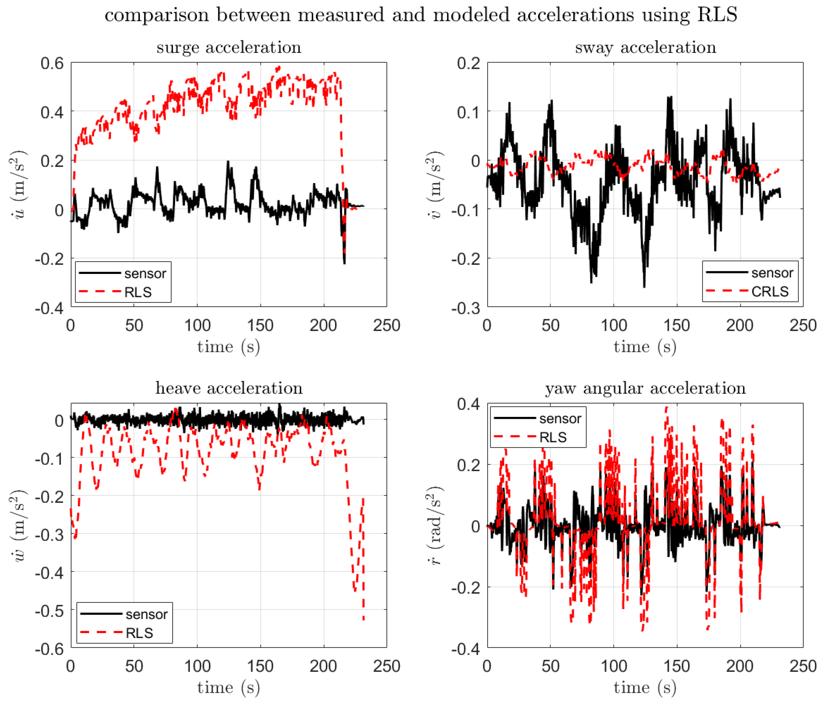
Figure 13 presents the comparison between the S-shape motion data and the RLS model. The analysis shows that the RLS based estimation for the S-shape dataset exhibited generally low reliability with considerable errors. In particular, the bias compensation capability was found to be significantly inferior compared to the CRLS. These results clearly demonstrate that in environments with inherent noise and bias, applying the CRLS method is far more effective than relying solely on the conventional RLS.
Overall, the CRLS-based dynamic model effectively tracked the measured linear and angular accelerations under various motion conditions, including the unified dataset, free-running, and S-shaped maneuvers dataset. The model achieved satisfactory RMSE and MAE values across most DoF, with particularly high accuracy observed in the heave direction. Even under high-frequency or transient conditions, the model maintained an acceptable level of predictive performance. These results indicate that the CRLS algorithm successfully captures the dynamic characteristics of the underwater vehicle.

3.3.3. Simulation with PID Controller

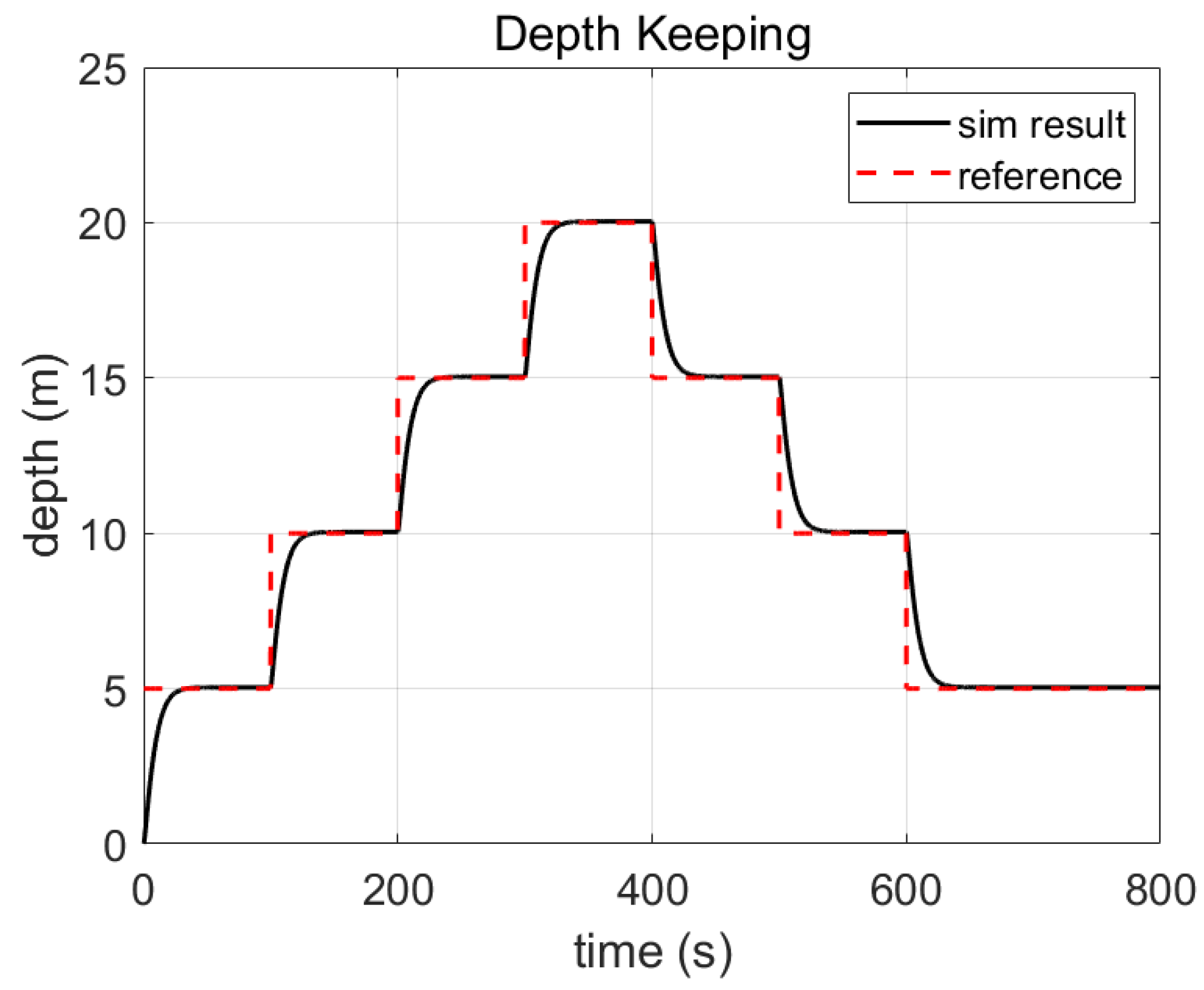
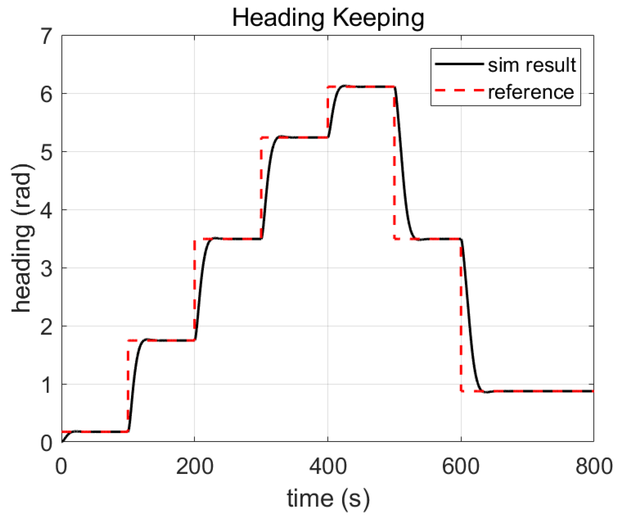
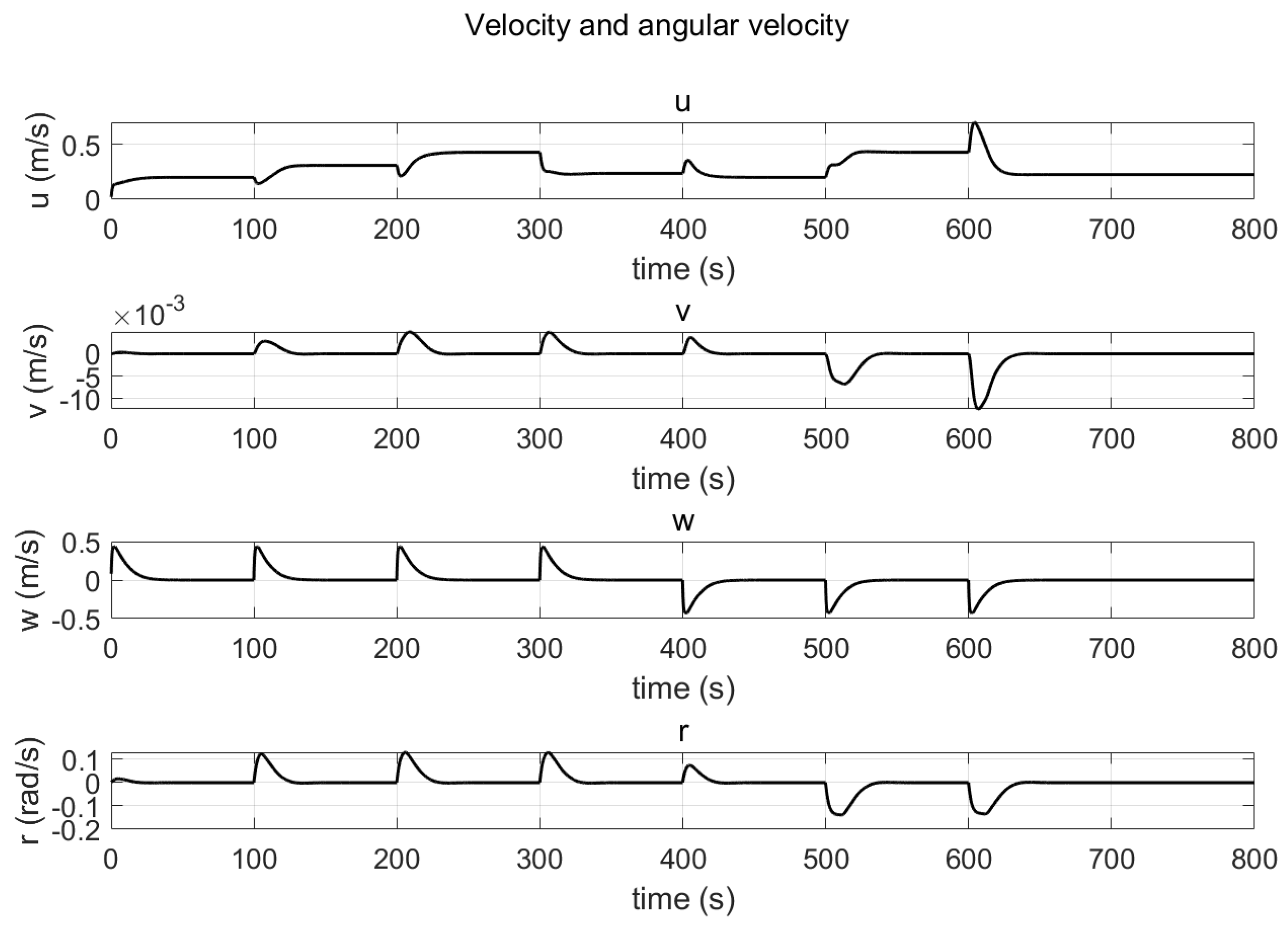
The control performance was evaluated through simulations using the validated coefficients of the P-SUROII. To investigate the dynamic performance, the reference values were varied over time while the vehicle moved in the forward direction. After applying a constant surge force to the P-SUROII, the depth and heading keeping were performed using PID controllers, and the results are presented in Figure 14, Figure 15 and Figure 16.
Figure 14 illustrates the depth control results. The reference depth trajectory was varied sequentially as 5, 10, 15, 20, 15, 10, and 5 m over time. The PID controller exhibited fast responses with negligible tracking errors to the step changes. After the initial transient, the system stably converged to the target depth with minimal overshoot. These results demonstrate that the PID controller designed based on the identified model ensures sufficient stability and accuracy in vertical motion control.
Figure 15 presents the heading control results. The reference heading trajectory was varied over time as 0.17, 1.74, 3.49, 5.23, 6.10, 3.49, and 0.87 rad. The PID controller demonstrated smooth tracking performance for the step-like reference inputs. Although a slight transient delay was observed during the yaw angle changes, the steady-state error was nearly negligible. These results confirm the effectiveness of the PID controller based on the identified parameters in the horizontal plane motion control.
Additionally, the velocity and angular velocity responses were analyzed, as shown in Figure 16, to examine the dynamic characteristics during attitude control. The surge velocity u exhibited small oscillations depending on the depth and heading control actions but converged stably. The sway velocity v remained at the order of 10 3 m / s , indicating that unintended lateral motions were effectively suppressed during the control process. The heave velocity w and yaw rate r also showed transient oscillations in response to changes in reference values but quickly stabilized thereafter. These results demonstrate that while control inputs may induce local oscillations, the overall system maintained stable control performance. These results support that the parameter estimation based on the proposed model was appropriately performed and demonstrate that the identified parameters accurately reflect the dynamic characteristics of the actual system.

4. Conclusions

In this study, an SI methodology based on the CRLS method is proposed to accurately estimate the dynamic parameters of the underwater robot P-SUROII. Considering the inherently passive stability of underwater vehicles in roll and pitch motions, modeling was performed for the remaining four DoF: surge, sway, heave, and yaw. To improve the accuracy of the input signals, dedicated experiments were conducted to quantify the thruster outputs. Based on these results, a comprehensive experimental dataset was constructed, incorporating forward, lateral, rotational, and vertical motion components.
To validate the effectiveness of the identified parameters, various motion experiments such as free-running and S-shaped maneuvers were utilized, and the model-based responses were compared with the measured data. Similarity metrics, including the RMSE and MAE, were used to quantitatively evaluate the agreement between the model and the sensor signals. As a result, under free-running conditions, the estimated model demonstrated low estimation errors in the surge axis, with RMSE = 0.0465 and MAE = 0.0339, thereby accurately reproducing the actual dynamic behavior. Furthermore, stable and consistent estimation performance was also achieved in the yaw axis. Under S-shaped maneuvering conditions, the model maintained comparable accuracy, yielding RMSE = 0.0470 and MAE = 0.0304 in the surge axis, while the yaw axis similarly exhibited reliable error levels. In contrast, the heave axis showed relatively larger errors (RMSE = 0.0745, MAE = 0.0571) due to external disturbances; however, the overall estimation performance remained reliable. Although minor discrepancies were observed in sections with abrupt motion changes, these errors were deemed acceptable for control applications.
Furthermore, PID simulations were conducted using the identified parameters, and it was confirmed that the depth and heading keeping control performance was well maintained. This verifies that the identified parameters effectively capture the dynamic characteristics of the actual system.
In conclusion, the CRLS-based identification method proposed in this study can be effectively applied to the dynamic modeling of underwater robots and can also be utilized for the implementation of simulators that support the design of high-performance controllers and the development of autonomous operating systems in complex marine environments. Furthermore, the estimated parameters can be incorporated into advanced control frameworks such as Model Predictive Control (MPC), contributing to the derivation of optimal control inputs while considering system dynamics and constraints. This enables robust and efficient performance in complex maneuvering tasks, including path following and collision avoidance.

Author Contributions

Conceptualization, H.K. and J.-H.L.; methodology, H.K. and J.-H.L.; software, H.K. and H.J.; hardware implementation and testing, H.K., M.-G.K. and M.-J.L.; validation and formal analysis, H.K., J.-H.L. and G.R.C.; investigation, H.K. and H.J.; data curation, H.K. and J.-H.L.; writing—original draft preparation, H.K.; writing—review and editing, H.K., J.-H.L. and S.J.; visualization, H.K. and J.-H.L.; supervision, H.K.; project administration, H.K. All authors have read and agreed to the published version of the manuscript.

Funding

This research was supported by the Korea Institute of Marine Science & Technology Promotion (KIMST), funded by the Ministry of Oceans and Fisheries, Korea, through the projects RS-2024-00432366 and RS-2023-00256122.

Data Availability Statement

The datasets presented in this article are not readily available because of institutional restrictions. Requests to access the datasets should be directed to the corresponding author.

Conflicts of Interest

The authors declare no conflicts of interest.

References

  1. Cho, G.R.; Kang, H.; Lee, M.J.; Li, J.H. Heading control of uri-t, an underwater cable burying rov: Theory and sea trial verification. J. Ocean Eng. Technol. 2019, 33, 178–188. [Google Scholar] [CrossRef]
  2. Kang, H.; Cho, G.R.; Kim, M.G.; Lee, M.J.; Li, J.H.; Kim, H.S.; Lee, H.; Lee, G. Mission management technique for multi-sensor-based AUV docking. J. Ocean Eng. Technol. 2022, 36, 81–193. [Google Scholar] [CrossRef]
  3. Castillo-Zamora, J.J.; Camarillo-Gómez, K.A.; Pérez-Soto, G.I.; Rodríguez-Reséndiz, J.; Morales-Hernández, L.A. Mini-AUV hydrodynamic parameters identification via CFD simulations and their application on control performance evaluation. Sensors 2021, 21, 820. [Google Scholar] [CrossRef] [PubMed]
  4. Ji, D.; Wang, R.; Zhai, Y.; Gu, H. Dynamic modeling of quadrotor AUV using a novel CFD simulation. Ocean Eng. 2021, 237, 109651. [Google Scholar] [CrossRef]
  5. Go, G.; Ahn, H.T. Hydrodynamic derivative determination based on CFD and motion simulation for a tow-fish. Appl. Ocean Res. 2019, 82, 191–209. [Google Scholar] [CrossRef]
  6. Safari, F.; Rafeeyan, M.; Danesh, M. Estimation of hydrodynamic coefficients and simplification of the depth model of an AUV using CFD and sensitivity analysis. Ocean Eng. 2022, 263, 112369. [Google Scholar] [CrossRef]
  7. Jeong, J.H.; Ok, J.H.; Lee, C.S.; Lee, J.M.; Lee, S.K. Estimation of hydrodynamic derivatives and dynamic stability for submarine using captive model test. J. Navig. Port Res. 2015, 39, 173–178. [Google Scholar] [CrossRef]
  8. Jung, J.W.; Jeong, J.H.; Kim, I.G.; Lee, S.K. Estimation of hydrodynamic derivatives of submarine model by using VPMM test. J. Navig. Port Res. 2014, 38, 97–103. [Google Scholar] [CrossRef]
  9. Kim, D.J.; Lee, G.J.; Kwon, C.S.; Kim, Y.G.; Park, J.Y.; Jun, B.H. Added mass of submerged bodies obtained by forced oscillation tests and numerical calculations of potential flow. J. Soc. Nav. Archit. Korea 2022, 59, 214–224. [Google Scholar] [CrossRef]
  10. Cardenas, P.; de Barros, E.A. Estimation of AUV hydrodynamic coefficients using analytical and system identification approaches. IEEE J. Ocean. Eng. 2019, 45, 1157–1176. [Google Scholar] [CrossRef]
  11. Jones, D.A.; Clarke, D.B.; Brayshaw, I.B.; Barillon, J.L.; Anderson, B. The Calculation of Hydrodynamic Coefficients for Underwater Vehicles; Technical Report; Citeseer: University Park, PA, USA, 2002. [Google Scholar]
  12. De Barros, E.; Pascoal, A.; De Sa, E. Investigation of a method for predicting AUV derivatives. Ocean Eng. 2008, 35, 1627–1636. [Google Scholar] [CrossRef]
  13. Johnson, M.L.; Faunt, L.M. [1] Parameter estimation by least-squares methods. In Methods in Enzymology; Elsevier: Amsterdam, The Netherlands, 1992; Volume 210, pp. 1–37. [Google Scholar]
  14. Dinç, M.; Hajiyev, C. Identification of hydrodynamic coefficients of AUV in the presence of measurement biases. Proc. Inst. Mech. Eng. Part M J. Eng. Marit. Environ. 2022, 236, 756–763. [Google Scholar] [CrossRef]
  15. Young, P.C. Recursive least squares estimation. In Recursive Estimation and Time-Series Analysis: An Introduction for the Student and Practitioner; Springer: Berlin/Heidelberg, Germany, 2011; pp. 29–46. [Google Scholar]
  16. Karras, G.C.; Marantos, P.; Bechlioulis, C.P.; Kyriakopoulos, K.J. Unsupervised online system identification for underwater robotic vehicles. IEEE J. Ocean. Eng. 2018, 44, 642–663. [Google Scholar] [CrossRef]
  17. Moore, J.B.; Weiss, H. Recursive prediction error methods for adaptive estimation. IEEE Trans. Syst. Man, Cybern. 1979, 9, 197–205. [Google Scholar] [CrossRef]
  18. Garnier, H.; Mensler, M.; Richard, A. Continuous-time model identification from sampled data: Implementation issues and performance evaluation. Int. J. Control 2003, 76, 1337–1357. [Google Scholar] [CrossRef]
  19. Wu, C.J. 6-Dof Modelling and Control of a Remotely Operated Vehicle. Ph.D. Thesis, College of Science and Engineering, Flinders University, Adelaide, Australia, 2018. [Google Scholar]
  20. Li, J.H.; Lee, M.J.; Park, S.H.; Kim, J.T.; Kim, J.G.; Suh, J.H. Development of p-SURO II hybrid autonomous underwater vehicle and its experimental studies. J. Inst. Control. Robot. Syst. 2013, 19, 813–821. [Google Scholar] [CrossRef]
  21. Fossen, T.I. Guidance and Control of Ocean Vehicles; Wiley and Sons: Hoboken, NJ, USA, 1994. [Google Scholar]
  22. Kim, J.; Chung, W.K. Accurate and practical thruster modeling for underwater vehicles. Ocean Eng. 2006, 33, 566–586. [Google Scholar] [CrossRef]
  23. Li, J.H.; Kim, M.G.; Kang, H.; Lee, M.J.; Cho, G.R. UUV Simulation Modeling and its Control Method: Simulation and Experimental Studies. J. Mar. Sci. Eng. 2019, 7, 89. [Google Scholar] [CrossRef]
  24. Li, J.H.; Kim, M.G.; Kang, H.; Lee, M.J.; Cho, G.R.; Kang, S. Initial alignment and position aiding time delay compensation for SDINS of deep sea underwater vehicles. In Proceedings of the 2022 American Control Conference (ACC), Atlanta, GA, USA, 8–10 June 2022; IEEE: Piscataway, NJ, USA, 2022; pp. 3126–3131. [Google Scholar]
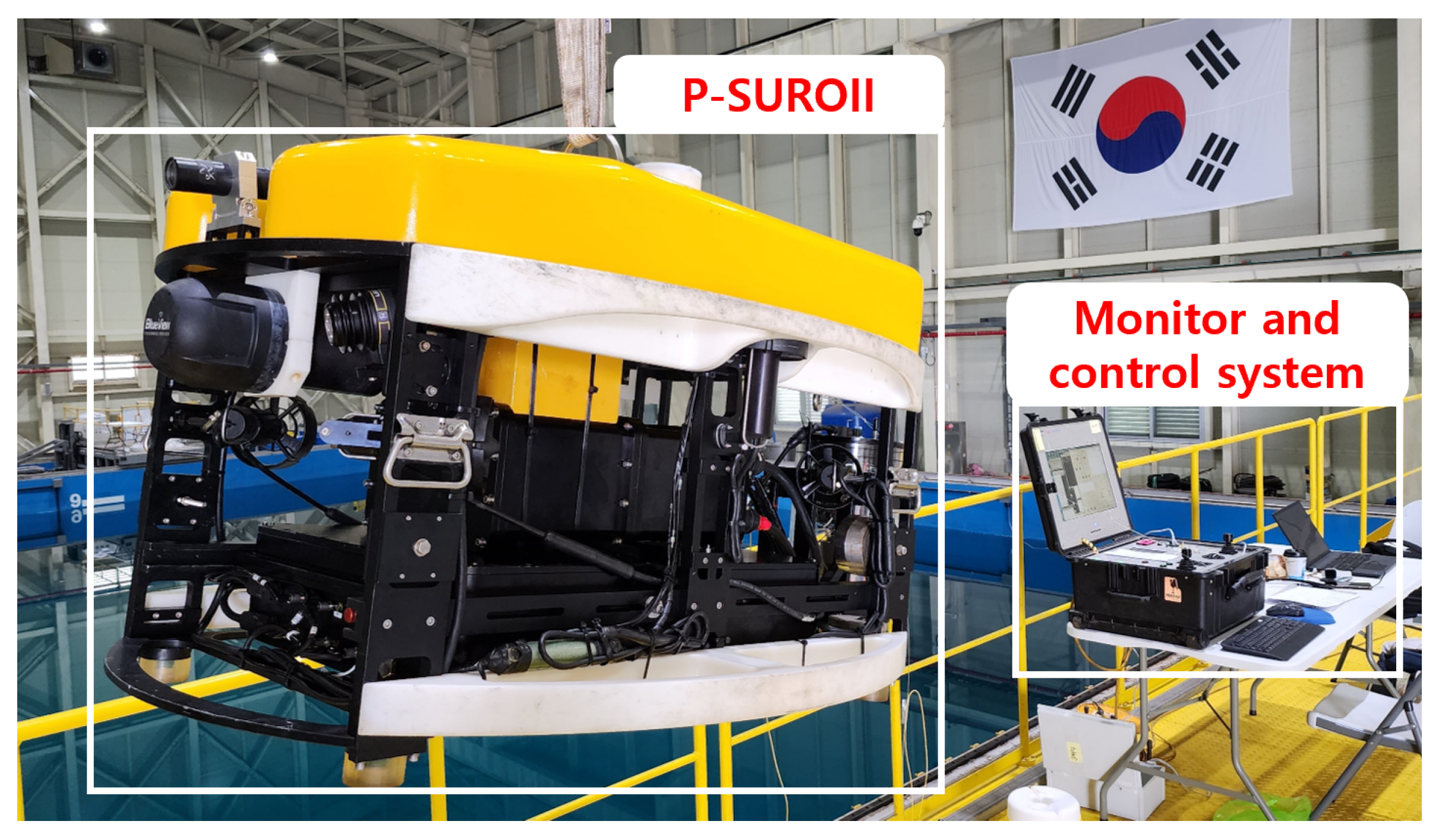
Figure 1. External appearance of P-SUROII.
Jmse 13 01610 g001
Figure 2. Configuration of P-SUROII.
Jmse 13 01610 g002
Figure 3. Coordinate system of P-SUROII.
Jmse 13 01610 g003
Figure 4. Experimental setup for thruster modeling.
Jmse 13 01610 g004
Figure 5. Measured and modeled thrust responses for thrusters. Each subfigure corresponds to the respective thruster and direction listed in Table 2 (e.g., the curve for Thruster ID 11 (Forward) corresponds to the “ID 11 forward” parameters in Table 2).
Jmse 13 01610 g005
Figure 6. The control input used in the simulation.
Jmse 13 01610 g006
Figure 7. Data acquisition test for SI in water tank.
Jmse 13 01610 g007
Figure 8. Control input for the unified data.
Jmse 13 01610 g008
Figure 9. Comparison between unified dataset and model data for CRLS.
Jmse 13 01610 g009
Figure 10. Comparison between free running dataset and model data for CRLS.
Jmse 13 01610 g010
Figure 11. Comparison between free running dataset and model data for RLS.
Jmse 13 01610 g011
Figure 12. Comparison between S-shaped dataset and model data for CRLS.
Jmse 13 01610 g012
Figure 13. Comparison between S-shaped dataset and model data for RLS.
Jmse 13 01610 g013
Figure 14. Depth control performance using PID.
Jmse 13 01610 g014
Figure 15. Heading control performance using PID.
Jmse 13 01610 g015
Figure 16. Velocity and angular velocity responses under PID control.
Jmse 13 01610 g016
Table 1. Technical specifications of P-SUROII.
ItemSpec
Size0.76 (H), 0.91 (W), 1.473 (L) (m)
Weight214.69 (kg)
SpeedMax. 0.5 (m/s)
SensorsDVL (Teledyne, pathfiner)
IMU (Fiberpro, FI200P)
AHRS (Microstrain, 3DM-GX5-25)
Pressure (Keller, 36XW)
Sonar (Blueview, P900)
Thruster (Seabotix, HPDC1521/1513)
Table 2. Coefficients for each thruster in forward and reverse directions.
Thruster T | n | n
(Forward)
T | n |
(Forward)
T | n | n
(Reverse)
T | n |
(Reverse)
ID 11 2.889 × 10 6 6.3166 × 10 4 2.614 × 10 6 6.5532 × 10 4
ID 12 2.778 × 10 6 8.161 × 10 4 2.595 × 10 6 7.4158 × 10 4
ID 31 2.796 × 10 6 8.1815 × 10 4 2.592 × 10 6 7.8458 × 10 4
ID 32 2.842 × 10 6 10.895 × 10 4 2.510 × 10 6 6.0624 × 10 4
Table 3. Comparison of hydrodynamic coefficients and added mass terms from CRLS and reference values.
Hydrodynamic Coefficients for TranslationalHydrodynamic Coefficients for Rotational
ItemUnitCRLSReferenceErrorItemUnitCRLSReferenceError
X u N·s/m−3.8404−4.03−0.1896 K p N·m·s/rad0−0.07−0.07
X u | u | N·s/m−18.8662−18.180.6862 K p | p | N·m·s/rad−1.2878−1.55−0.2622
X u ˙ kg−5.2189−5.5−0.2811 K p ˙ kg·m−0.1314−0.120.0114
Y v N·s/m−6.4987−6.220.2787 M q N·m·s/rad0−0.07−0.07
Y v | v | N·s/m−18.5199−21.66−3.1401 M q | q | N·m·s/rad−2.9542−1.551.4042
Y v ˙ kg−8.7398−12.7−3.9602 M q ˙ kg·m−0.1452−0.120.0252
Z w N·s/m−6.2698−5.181.0898 N r N·m·s/rad−0.1−0.070.03
Z w | w | N·s/m−22.0082−36.99−14.9818 N r | r | N·m·s/rad−1.3841−1.55−0.1659
Z w ˙ kg−12.4941−14.57−2.0759 N r ˙ kg·m−0.094−0.12−0.026
Table 4. Main physical parameters of the P-SUROII.
ParameterValue
Total mass, m 214.69 kg
Center of gravity (CoG) ( 0 , 0 , 0.11 ) m
Center of buoyancy (CoB) ( 0 , 0 , 0 ) m
Moment of inertia, I x x 20.56421 kg · m 2
Moment of inertia, I y y 37.1049 kg · m 2
Moment of inertia, I z z 3.259221 kg · m 2
Table 5. Hydrodynamic parameters for each motion equation.
Surge DirectionSway DirectionHeave DirectionYaw Direction
ItemUnitValueItemUnitValueItemUnitValueItemUnitValue
X u kg/s80.00 Y v kg/s175.77 Z w kg/s130.05 N r kg· m 2 /s23.59
X u | u | kg/m150.00 Y v | v | kg/m255.38 Z w | w | kg/m204.64 N r | r | kg·m22.42
X u ˙ kg25.50 Y v ˙ kg12.70 Z w ˙ kg99.50 N r ˙ kg· m 2 34.22
Disclaimer/Publisher’s Note: The statements, opinions and data contained in all publications are solely those of the individual author(s) and contributor(s) and not of MDPI and/or the editor(s). MDPI and/or the editor(s) disclaim responsibility for any injury to people or property resulting from any ideas, methods, instructions or products referred to in the content.