Abstract
Multi-vessel formation shipping demonstrates significant potential for enhancing maritime transportation efficiency and economy. However, existing route planning systems inadequately address the unique challenges of formations, where traditional methods fail to integrate global optimality, local dynamic obstacle avoidance, and formation coordination into a cohesive system. Global planning often neglects multi-ship collaborative constraints, while local methods disregard vessel maneuvering characteristics and formation stability. This paper proposes GLFM, a three-layer hierarchical framework (global optimization–local adjustment-formation collaboration module) for intelligent route planning of transport ship formations. GLFM integrates an improved multi-objective A* algorithm for global path optimization under dynamic meteorological and oceanographic (METOC) conditions and International Maritime Organization (IMO) safety regulations, with an enhanced Artificial Potential Field (APF) method incorporating ship safety domains for dynamic local obstacle avoidance. Formation, structural stability, and coordination are achieved through an improved leader–follower approach. Simulation results demonstrate that GLFM-generated trajectories significantly outperform conventional routes, reducing average risk level by 38.46% and voyage duration by 12.15%, while maintaining zero speed and period violation rates. Effective obstacle avoidance is achieved, with the leader vessel navigating optimized global waypoints and followers maintaining formation structure. The GLFM framework successfully balances global optimality with local responsiveness, enhances formation transportation efficiency and safety, and provides a comprehensive solution for intelligent route optimization in multi-constrained marine convoy operations.
1. Introduction
With the rapid development of global trade, ship transport is the main way of international trade. According to the International Maritime Organization (IMO), the total amount of goods transported by sea each year exceeds 10 billion tons, accounting for more than 80% of the total global trade [1]. The efficiency and economy of ship transport make it an indispensable link in the global supply chain. However, traditional single-ship operations face increasing challenges from complex maritime environments and large-scale demands, exhibiting limitations in efficiency, safety, and flexibility. In order to cope with these challenges, multi-ship formation shipping, as a new shipping mode, is receiving more and more attention. Multi-ship formation shipping can greatly improve the transportation efficiency and economy through the cooperative operation of multiple ships, which has become an important direction of the future development of the shipping industry [2].
Effective navigation for such formations in dynamic and complex sea environments (characterized by severe weather, ocean currents, waves, and navigational hazards like reefs, wrecks, and other traffic) hinges on intelligent route planning [3,4]. This planning must concurrently ensure global path optimality (minimizing time, risk, fuel), local dynamic obstacle avoidance (reacting to unforeseen obstacles while considering ship dynamics), and stable formation coordination (maintaining safe inter-vessel distances, synchronized speeds, and structural integrity during maneuvers). However, current trajectory planning methodologies exhibit critical shortcomings in formation scenarios:
- Global Planning Limitations: Conventional global algorithms (e.g., A*, Dijkstra, evolutionary algorithms [5,6,7,8,9,10,11,12,13,14,15,16]) often utilize single or fixed-weight objectives. They fail to adequately incorporate dynamic METOC factors, IMO safety rules, and crucially, the spatiotemporal constraints essential for multi-vessel coordination (e.g., synchronized path execution, safe separation assurance) [17]. Multi-objective variants like MOA* still struggle with balancing complex objectives and enforcing hard safety constraints in formation contexts.
- Local Obstacle Avoidance and Formation Control Deficiencies: In order to cope with the change in local dynamic environment, scholars have put forward a variety of local track planning methods [18,19,20,21,22,23,24,25]. Local methods like Artificial Potential Field (APF), while responsive, suffer from inherent issues like local minima and oscillations, and often lack integration of ship-specific maneuvering characteristics and safety domains. As for how to maintain formation stability, researchers have proposed a variety of formation methods, such as the leader–follower method [26,27], the virtual structure method [28,29], and the behavior-based method [30,31], inspired by the behaviors of birds gathering, ant colonies, and bee colonies. Formation control strategies, predominantly leader–follower (LF) for its simplicity, frequently rely on idealized ship dynamics, lack robustness to leader failure, exhibit poor compatibility with heterogeneous vessel performance, and pose collision risks during maneuvers like turns.
Consequently, the synergistic mechanisms integrating global planning, local adjustment, and formation collaboration remain fragmented, lacking an organic unified framework capable of addressing the intertwined challenges of efficiency, safety, and coordination in transport ship formations. High-profile incidents like the 2021 Suez Canal grounding of the MV Ever Given, which caused massive global trade disruption, underscore the critical need for advanced, integrated planning solutions.
These studies have yielded some results. However, a more complete and accurate route intelligent optimization system is needed for multi-constrained ship formation sailing. The path planning and cooperative control of multi-ship formation shipping can be summarized into two parts: First, the global path planning is based on the known environmental information to plan the route from the starting point to the target point; the other is local track planning using sensors to detect the local environment in real time. The small dynamic obstacles are identified and avoided, and the ships in the formation form a stable structure to coordinate the control of the formation. It is worth paying attention to the development of ship domain theory, which provides a new idea for dynamic collision avoidance and formation structure by establishing a two-dimensional ellipsoid model to quantify the safe distance between ships. In addition, the meteorological and marine environment is a problem that must be considered in the whole system. In the field of ships, the meteorological and marine environment will greatly affect the effectiveness of the model.
Motivated by these challenges, this paper presents the GLFM (Global–Local-Formation Module) framework, a hierarchical three-layer architecture designed for intelligent route planning of transport ship formations. The main contributions are as follows:
- A novel hierarchical planning framework (GLFM) integrating global optimization, local dynamic adjustment, and formation coordination layers for autonomous and cooperative navigation of transport vessel formations in complex environments.
- An enhanced multi-objective A* algorithm for global route planning under dynamic METOC conditions. This algorithm incorporates environmental risk and time cost functions with dynamic weighting, and rigorously enforces safety constraints based on IMO regulations, bathymetry, land boundaries, and start/end points, yielding safer and more stable global paths.
- An improved dynamic local obstacle avoidance strategy combining an enhanced APF method with ship safety domain models. Global waypoints and constraint-based techniques are leveraged to mitigate APF drawbacks (local minima, oscillations). Formation stability and coordination are achieved via an improved leader–follower approach, augmented with artificial potential fields and safety fields to prevent inter-ship collisions during cooperative control, addressing inherent LF limitations.
The remainder of this paper is organized as follows: Section 2 describes the data sources and methodologies employed. Section 3 analyzes the spatiotemporal characteristics of the wind–wave environment in the study area. Section 4 details the system model formulation. Section 5 presents simulation results and analysis for global planning, local adjustment, and formation cooperation. Section 6 concludes the study.
2. Data and Methods
2.1. Data
The study area of this paper is marine transportation in the North Pacific, so this paper uses the meteorological and marine environmental data of this Pacific region for analysis. The historical data range used is 0° N–47° N, 120° E–100° W. The wave data is three-dimensional grid data from the Copernicus Marine Environmental Monitoring Service Network (CMEMS), all using sea surface data. Sea wave includes effective wave height, mean period, wave direction, wind wave height, wind wave direction, swell wave height, and swell wave direction. The spatial resolution of the grid is 1/12° × 1/12°. Surface wind field and surface pressure 3D grid data were obtained from the Copernicus Atmospheric Monitoring Service (CAMS), using ten meters of surface data. Wind field includes two aspects: wind direction and wind speed. The spatial resolution of the grid is 1/12° × 1/12°. The depth data for the North Pacific Ocean is derived from the NGDC’s ETOPO1 dataset, which contains ocean floor topographic data with a spatial resolution of 1′ × 1′. The temporal resolution of all data is 1 h of data.
The research object selected in this paper is a large container ship, and its basic performance parameters are shown in Table 1:

Table 1.
Basic parameters of large container ships.
2.2. Methods
In order to study the navigation safety of container ships (Jinchuan Shipbuilding Co., LTD, Hangzhou, China) in the meteorological ocean environment, the environmental factors such as wind, wave, and pressure in winter and summer in the North Pacific Ocean are compared and analyzed. The dynamic changes in strength and direction of different elements and their interaction are considered. The optimal route for ship navigation safety is studied when the wind and waves are high. The cost function of the A* algorithm is used to coordinate these three different objective functions. Given the weights of different objective functions, a route focusing on one aspect can be obtained. In addition, safety restrictions such as the IMO have been added to avoid extremely dangerous waters. In this paper, the safety domain of the ship is obtained by the scale parameters of the ship and the elements of the air–sea environment. Combined with the artificial potential field method, the algorithm model of ship avoiding obstacles is given. The A* algorithm is used to plan local target points to make up for the defects of the artificial potential field method. Based on the leader-following method and synthetic artificial potential field, the stability of the formation structure is maintained to ensure that each ship does not deviate from the overall navigation route and avoid mutual influence between each ship. The overall method structure of this paper is shown in Figure 1.
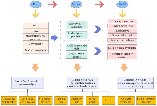
Figure 1.
Basic flow chart of this study.
3. Analysis of Wind and Wave Elements in the North Pacific
The changes in the wind and wave field in the North Pacific are remarkable. Wind speeds and waves are much higher in winter than in summer. And high winds and waves are much more frequent. Not only that, but the difference in the degree of wind waves in different seas at different times in the same season is also relatively large. By analyzing the prevailing wind speed, wind direction, wave height, wave direction, and the frequency of large waves, the basic characteristics of the wind wave field in the North Pacific Ocean in different periods are studied. It provides reference data and variation rules of the wind and wave field for ship formation sailing in the North Pacific Ocean.
3.1. Characteristics of Wind and Wave Dynamics in Winter
The winter monsoon season brings a much higher frequency of severe winds and waves to the North Pacific compared to other seasons, with January being the peak month for the strongest wind and wave activity. In the North Pacific region throughout January, the wind speed of more than eight winds accounted for more than 4% and the wave height of more than 6 m accounted for more than 2%. The average maximum wind speed in January is about 14 m/s, and the average maximum wave height is about 5 m. The overall distribution is shown in Figure 2:
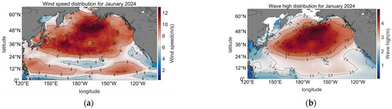
Figure 2.
Average wind wave distribution over the North Pacific Ocean in January. (a) Average wind speed in the North Pacific Ocean in January. (b) Average wave height in the North Pacific Ocean in January.
It can be seen from Figure 2 that the average wind speed in most parts of the North Pacific region is above 8 m/s, and the average wave height is above 3 m. Its distribution is smaller in the equatorial region and larger in the northern region. Among them, the average wind speed between 10° N and 24° N is also large, basically above 8 m/s. And the maximum is 12 m/s. For waves centered in the Aleutian Islands, this area has the highest wave height, reaching 5 m. Its intensity gradually decreases to the Bering Strait in the north, the Hawaiian Islands in the south, Japan in the east, and the Gulf of Alaska in the west, with an average wave height of more than 3 m. The average wave height in the 10° N~24° N wind speed area is also about 2.5 m, and the rest of the wave height near the equator and near the coastline is below 2 m.
The intensity and directional frequency of January winds and waves for this region are shown in Figure 3:
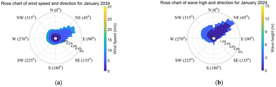
Figure 3.
Rose chart of wind wave intensity and direction in the North Pacific Ocean in January. (a) Wind speed and direction in the North Pacific in January. (b) Wave height and direction in the North Pacific in January.
It can be seen from the figure that the direction of the wind in the whole of January is mainly in the direction of NE to E, and its frequency accounts for about 34%. Other winds in each direction also account for about 1–2%. In January, the proportion of waves in the direction of NE is relatively high, accounting for about 34% of the whole. In addition, there are also a lot of waves from the SW direction to the N direction, accounting for about 32.5% of the whole. The rest of the direction of the wave accounted for less, at about 24% of the state of no waves.
3.2. Characteristics of Wind Wave in Summer
The summer monsoon period marks the calmest wind and wave conditions of the year, with July being the calmest month. The average wave height is the smallest, with a low frequency and small extent of high waves. In the North Pacific region, the occurrence of winds above Beaufort scale 8 in July is only about 0.08%, while the proportion of waves exceeding 6 m in July is approximately 0.009%. In July, the monthly average maximum wind speed is around 10 m/s, and the monthly average maximum wave height is about 2.4 m. The overall distribution is shown in Figure 4:
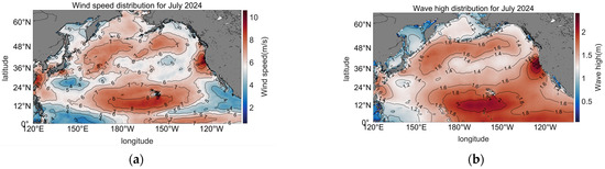
Figure 4.
Distribution map of mean wind waves in the North Pacific Ocean in July. (a) Average wind speed in the North Pacific in July. (b) Average wave height in the North Pacific Ocean in July.
It can be seen from Figure 4 that half of the average wind speed in the North Pacific region is about 6 m–7 m. Average wind speeds above 8 m/s (but below 10 m/s) are limited to the region between 10° N~14° N and 170° E~160° W, along with a small area off San Francisco’s east coast. In areas with an average wind speed of 8 m/s, wave heights reach 2 m, while elsewhere wave heights are approximately 1.5 m, suggesting that swells play a major role.
The intensity and directional frequency of wind and waves in July for this region are shown in Figure 5:
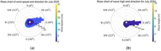
Figure 5.
Rose chart of wind wave intensity and direction in the North Pacific Ocean in July. (a) Wind speed and direction in the North Pacific in July. (b) Wave height and direction in the North Pacific in July.
Figure 5 shows that in July, winds mainly blow from NE to SE, accounting for about 44%, with other directions each contributing 1.6% to 2%. Waves predominantly come from the E direction (36%), while SE to SW directions each account for around 2%. Waves from other directions are rare, and 22.4% of the time is calm (no waves).
3.3. Characteristics of Wind and Wave at the Time When Wind and Wave Are Stronger in Winter
This study focuses on optimizing shipping routes for container ship fleet safety, selecting January as the research period due to its strong wind and wave conditions. Analyzing wind/wave intensity and direction aids in route optimization. Figure 6 illustrates the wind/wave intensity, direction, and sea surface pressure at a selected time point with strong conditions.
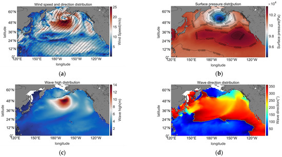
Figure 6.
Distribution of sea surface pressure, wind/wave intensity, and direction at a specific time point in the North Pacific during Winter. (a) Wind speed and direction in the North Pacific at a given time; (b) sea surface pressure in the North Pacific at a given time; (c) wave height in the North Pacific at a given time; (d) wave direction in the North Pacific at a given time.
From the figure, it can be observed that at this moment, there is an extremely strong low-pressure system over the Aleutian Islands in the North Pacific, with its central pressure as low as 950 hPa. In the eastern Pacific, there is a North Pacific high-pressure system, with its central pressure exceeding 1036 hPa. These two pressure systems significantly influence wind speed and direction. To the south of the Aleutian low-pressure system, there is a very strong gale system, with maximum wind speeds exceeding 25 m/s, rotating counterclockwise around the Aleutian Islands. Near the North Pacific high-pressure system, wind speeds are lower, but there are two regions of relatively high wind speeds to the northwest and northeast, rotating clockwise around the high-pressure center. Below 35° N, winds are predominantly northeasterly and easterly, while near the western coast, winds are northwesterly. The peak wave heights are concentrated to the south of the Aleutian low-pressure system, with the highest waves exceeding 14 m. The wave direction also rotates counterclockwise around the Aleutian Islands. Influenced by the wind speeds, in the region between 20° N and 50° N, waves are mainly northwesterly, moving from northwest to southeast. Below 20° N, waves are northeasterly, but beyond 120° W, they are northwesterly with swells dominating in this area.
The simulation experiment selects the period starting from 1 January as the background environment for average daily data. Such selection can give the final results a higher contrast. Using daily average data reduces the computational requirements for subsequent segmented simulations. Therefore, when the environment is relatively calm, the model can still compute corresponding results. Additionally, when sufficient computational resources are available, it can calculate results for more frequent, higher temporal-resolution hydrometeorological changes.
4. The Establishment of System Model
4.1. Impact Model of Environmental Factors
Large container ships have large tonnage and large inertia, which will greatly affect the navigation safety of ships under the interference of a harsh environment. Generally, the influence of sea wind and waves is relatively high. This study considers only the effects of sea wind and wave intensity on ship handling safety, their intensity and direction on speed, and wave period on rolling resonance.
4.1.1. Impact on Ship Maneuvering Safety
Sea wind primarily acts on the area above the ship’s waterline and is related to wind speed, wind direction, and spectral density. The wind force acting on the ship is given [32] as follows:
where is the windward area of the ship along the and directions. is the wind speed in the and directions. is the spectral density of sea wind. is the pulsating wind frequency.
The force model of ocean waves is as follows [32]:
where is related to the stressed area of the ship. is the average wave wavelength. and are the components of the wave in the and directions. is the wave frequency.
For simplicity, direction and period are considered separately. Here, only the intensity of wind and waves is taken into account. From the perspective of ship maneuvering, it is generally considered that wind forces reaching Beaufort scale 8 or higher, and wave heights exceeding 6 m, constitute a high-wind and rough-sea environment for large vessels. Such conditions are already quite hazardous. Based on this, sea wind and waves are classified into five risk levels according to their intensity (the wind- and wave-risk classification criteria in this paper are derived from a comprehensive consideration of supervisory data provided by multiple maritime authorities and the results of force-model simulations for wind and wave action), as shown in Table 2:
Table 2.
Risk classification table of wind and wave.
4.1.2. Influence of Ship Speed
Ships in the wind and waves will not maintain the ship’s driving speed, often resulting in a stall effect. The stall model was obtained by introducing the stalling factors of the sea wave and wind field [33].
where is the ship’s speed in still water. is the angle between the course and wave direction. is the wave height. is the wind speed. is the angle between the course and wind direction. is the ship’s displacement.
During navigation in heavy wind and waves, ships face risks such as hull slamming, deck wetness, and propeller racing due to wave impacts and severe rolling, which can lead to damage and reduced safety. To mitigate these dangers, ships must reduce their speed to a certain threshold, known as the critical speed. There are various methods to calculate the critical speed of ships under wind and wave conditions. Among them, Kitahara and Hosoda [34] derived the critical speed through extensive research on various ships under different sea states.
When the actual speed of the ship under the wind and waves is greater than the critical speed under the sea state, it should slow down to the critical speed to avoid danger.
4.1.3. Effects of Wave Period on Ship Resonance
The calculation formula of the wave encounter period given by IMO circular [35], combined with the period of ocean waves, is as follows:
When the ship’s natural rolling period is approximately 0.7 or 1.3 times the encountered wave period , resonance is highly likely to occur. This amplifies the ship’s rolling motion and increases the risk of capsizing. Therefore, ships should avoid operating within this range during navigation.
4.2. Sailing Time Model
To calculate the ship’s navigation time, it is necessary to determine the distance between two points in the gridded environmental field. Assuming the Earth is spherical, the sailing distance between two given points (, ), (, ) can be calculated using the following formula [4].
where is the radius of the Earth. The sailing time can be obtained according to the sailing distance and sailing speed between two points.
Navigation time for each step is computed by taking the distance between adjacent grid points on the route and incorporating local environmental values into the speed influence model.
4.3. Seabed Height Safety Model
The navigation of large vessels still requires consideration of seabed topography. The draft of a ship refers to the part of the hull below the water surface. If the water depth is insufficient, the ship may run aground, leading to hull damage or even capsizing. In shallow waters, waves and tides are more intense and maneuvering difficulties increase, such as challenges in steering, reduced speed, and increased hull vibrations. To ensure basic safety, ships must maintain a water depth greater than their draft, typically with an additional safety margin, which is generally more than 2 m for large vessels. Generally, water depths less than 1.5 times the draft are considered shallow water navigation, where ships are significantly affected by shallow water effects. Water depths between 1.5 and 2.5 times the draft are considered medium depth, where navigation is less affected, but changes in water depth still need attention. When the water depth exceeds 2.5 times the draft, the shallow water effects are minimal, and navigation safety is high.
Based on the empirical formula derived from model simulation experiments. Vessel’s safe water depth = vessel’s draft + a × significant wave height + b × speed + tidal error (where a and b are coefficients related to vessel type). Consequently, this paper primarily divides water depth into three components: when water depth is less than the draft depth, the model imposes a hard constraint, and vessels absolutely cannot navigate under such conditions; when water depth exceeds the draft depth but remains below the safe water depth, the specific depth value can be uniformly distributed into a 0~1 risk level, exerting certain influence on the model; and when water depth exceeds the safe water depth, the impact of water depth can be disregarded.
4.4. Ship Safety Distance Model
The study of ship safety distance is indispensable for surface ship formation to avoid obstacles or to form a stable formation. Ship safety distance, also known as the ship safety field, is a professional term widely used in the field of Marine engineering, such as collision and intersection. The ship domain was first proposed by Fujii and Tanaka [36] and is defined as “the two-dimensional area around a ship that other ships must avoid—it can be considered an escape area”. After years of development, different scholars have different understandings of the ship field. Nowadays, there are usually three research methods: empirical ship field model, knowledge-based ship field model, and analysis-based ship field model [37]. Based on the analysis of the dynamic quaternion ship model in a ship domain, this paper studies the safety domain of container ships. The proposed Dynamic Quaternion Ship Domain (DQSD) model is integrated by three independent sub-models of ship maneuverability, crew status and navigation, and meteorological and marine environment [38]. The method is based on the Quaternion Ship Domain (QSD) model, which contains a scale quaternion and shape parameter where represents the forward, aft, starboard, and port direction radii of the ship. The basic formula for adding meteorological and marine environmental factors after modification is as follows:
where represents the gain factor of meteorological and marine environmental elements on the forward, aft, starboard, and port direction radii. is the length of the ship. is the speed of the ship. The factor of the four directional radii generally has the influence of other ship elements. This section is carried out to simplify the main effects of ship length and ship speed. The shape parameter k is a factor affecting the status of the ship crew. It is important to note that the model is dynamic. For the same ship, the status of the crew and the meteorological and marine environment change with time, so the safety field of the ship applying this model also changes dynamically. Generally speaking, the relationship expression of crew status affecting the shape parameter k is as follows:
where is the various state parameters of the crew, such as operational skills, physical status, morale, and so on. The value can be [−1, 0] based on experience. is the weight indicator and the weight of each status parameter. are shape parameters and scale parameters, generally , .
The relationship expression of the impact factor of meteorological and marine environmental factors is as follows:
where is an artificially divided output variable. The value of is [1,5], ∈ {0.6, 0.8, 1.0, 1.2, 1.4}. is the influencing factor of the meteorological and marine environment. Different meteorological and marine environmental factors can be selected, and the impact factors can be normalized to 0~1 according to the actual environment. Set the weight to get .
Therefore, the ship’s safety domain is adjusted in real time according to the actual environment, ship type, and crew condition; within the model, it remains a hard constraint—regardless of how the domain changes, obstacles must never intrude into it, and the safety domains of different ships must never overlap.
4.5. Ship Anti-Collision Model
When a following vessel in a fleet gets too close to obstacles along the tracking path, there is a high risk of collision. Therefore, to address this situation, each following vessel in the fleet must independently implement local collision avoidance. This paper adopts the artificial potential field method to study ship obstacle avoidance. The core idea of the artificial potential field is to construct an attractive potential field towards the target and a repulsive potential field away from obstacles. Under the combined effect of attraction and repulsion, the vessel avoids obstacles and reaches the target point.
4.5.1. Basic Algorithm of Artificial Potential Field
When the distance between the ship and the target point is farther, the gravitational potential energy of the target point is greater. When the target point is reached, the gravitational potential energy is zero. Then the function expression of the gravitational potential field is as follows:
where the position of the target point is . The position of the ship is . is the gravitational gain coefficient. Gravity is the negative gradient of the gravitational field, and the direction is from the ship to the target point. Then, the gravitational function expression is
When the ship is outside a certain range of the obstacle, it will not be subjected to the repulsive potential energy of the obstacle. When the ship enters the influence area of the obstacle, the closer the distance is, the greater the repulsive potential energy of the obstacle. The function expression of the repulsive force potential field is
where the coefficient is the repulsive force gain coefficient, and is the distance between the ship and the obstacle. is the influence radius of the repulsive potential field of the obstacle, and the repulsive force beyond this range is zero. Then, the repulsion function expression is
Since the ship may be repulsed by more than one obstacle at a certain position, the resultant force obtained by the superposition of gravity and repulsion is
4.5.2. Defects and Improvements of Artificial Potential Field
The artificial potential field method has three main drawbacks: First, when the ship is too far from the target point or the gain coefficients for attraction and repulsion are inappropriate, the attraction force may become excessively large while the repulsion force is negligible, allowing obstacles to intrude into the ship’s safety zone or even causing collisions. Second, when obstacles are near the target point, the repulsion force is strong, and the attraction force is weak, making it difficult for the ship to reach the target. Third, when the repulsion force from obstacles and the attraction force from the target are equal in magnitude but opposite in direction, the ship may become trapped in a local optimum and fail to proceed further. In the maritime domain, environmental factors such as waves, currents, and wind significantly affect ship motion. Traditional artificial potential field models do not consider these factors, which may cause deviations in the generated paths during actual navigation, increasing the risk of collisions between ships and obstacles. Traditional artificial potential field models typically treat ships as point masses, neglecting the dynamic characteristics of vessels, such as inertia and acceleration limits. In practical navigation, a ship’s movement is constrained by its own propulsion system, making it impossible to instantly change speed or direction. As a result, paths generated by traditional models may not be executable by actual ships.
To address the shortcomings of the artificial potential field method, this paper utilizes the results of global path planning for correction. In practice, surface vessel fleets, based on global path planning, exhibit autonomous collision avoidance behavior when following vessels encounter obstacles. Once the vessel bypasses the obstacle, it returns to the fleet and continues along the planned trajectory. Therefore, when the target point is too far or too close to an obstacle, a new target point can be selected from the grid points of the A algorithm path, or a suitable point between two grid points can be chosen as the target. When the vessel reaches a local optimum, a virtual target point or obstacle can be introduced to add a new attractive or repulsive potential field, breaking the existing balance until the vessel reaches the target and rejoins the fleet. Alternatively, a new grid point from the A algorithm path can be selected to modify the attractive potential field. To account for the influence of marine environmental factors and ship parameters, the attraction and repulsion gain coefficients can be adjusted based on wind, wave, current conditions, and vessel motion states. This transforms fixed values into functions of environmental and ship parameters (), thereby modifying the attractive or repulsive force gain coefficients in the artificial potential field algorithm to resolve the local optimum problem. To ensure vessel safety and algorithm effectiveness, these measures may all lead to minor modifications of the globally planned trajectory points. This paper adjusts the APF gain parameters in accordance with the environment and actual conditions, thereby reinforcing the absolute hard constraint imposed by the ship domain model, ensuring both algorithmic safety and path smoothness, and consequently guaranteeing the universality of the algorithmic results.
4.6. Stability Model of Ship Formation Structure
It is of great significance to construct a formation structure to maintain structural stability for multi-ship navigation. Formation control ensures that all types of ships in the entire formation can achieve unified command, orderly action, and ensure the safety of navigation. In addition, stable formation control allows ships to return to formation after completing other tasks, such as obstacle avoidance alone. Fleet control involves the transition of each vessel from random positions to the formation structure, as well as maintaining the stability of the formation. In this paper, the leader-following method is used to study the cooperative control of the formation. The leader sails through the predetermined route, and the other ships follow the leader according to the distance and orientation of the leader to achieve the cooperative control of the whole formation. The leader’s route is planned using the A algorithm from the global path planning method. The followers’ actions incorporate the concept of the artificial potential field to determine the designated positions they need to reach and to avoid collisions among vessels during the formation process. The leader–follower algorithm is then used to guide the followers to their designated positions.
For formation control, not only the position information of the ship is considered, but also the reference speed and deviation angle are required. A basic model of a single ship can be shown in Figure 7. The linear speed of the ship is . Its angular velocity is . Its deviation angle is .
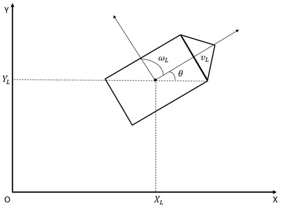
Figure 7.
Model diagram of a single ship.
Therefore, the kinematics model of a single ship is as follows:
The other ships in the formation can determine the ideal attitude of the future follower based on their own attitude information and that of the navigator. Figure 8 assumes the initial attitude information of the leader and the follower. The linear velocity of the follower is . Its angular velocity is . Its deviation Angle is . The linear distance between the leader and the follower is . The final deviation Angle that the follower needs to reach is .
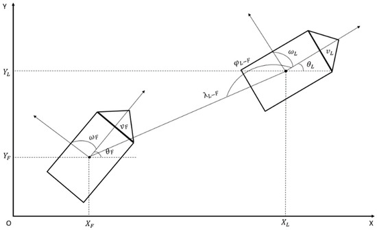
Figure 8.
Leader–follow formation structure model.
In the initial stage, the position relationship between followers and leaders is as follows:
The position relationship between the follower and the leader at the set ideal position is as follows:
The position relationship between the follower in the initial stage and the follower in the ideal position is as follows:
The error expression is as follows:
By substituting the relevant expression, the error expression is as follows:
In order for the follower to be able to follow the leader’s voyage in time, we must reduce the error value to 0. Thus, the error value affects the position, speed, and square of each follower. The stability of the queue is achieved by eliminating errors.
In the initial phase, each ship is in a random position. The formation consists of a leader and a number of followers. The relative position of each ship in the formation can be set in advance, so that multiple ships can form a fixed formation. The next position coordinates of the pilot are obtained from the coordinates planned by the A* algorithm. The next position information of the follower is determined by the combined force of the gravitational potential energy of the target position (the relative position of the follower to the leader) and the repulsive potential energy given by the other ships. The gravitational potential energy is determined by the distance between the follower’s present position and the target position. The potential energy of the repulsion force is determined by the distance between the ships. Then the position model for the next step of the follower is
where and are the coordinate positions of the k-th iteration. and are the relative positions of the follower with respect to the leader after the k + 1-th iteration. is the gravitational gain coefficient. is a binary value (0 or 1) after the k-th iteration. When the distance between ships is greater than the safe distance, is 0, indicating no collision risk, and the repulsive potential energy is not considered. When the distance between ships is less than the safe distance, is 1, indicating a potential collision, and the repulsive potential energy must be considered. represents the gradient of the repulsive potential energy after the k-th iteration:
where is the repulsion gain coefficient. is the minimum safe distance between ships. is the distance between two ships.
Using the leader–follow method, we must also consider two problems: First, when the difference between different ships in the formation is too large, the difference in inertia and rudder efficiency leads to the difficult unification of control parameters:
where is the captain and is the rudder efficiency factor. If the difference in ships in the formation exceeds 30%, a significant tracking error will be generated. The compatibility problem can be solved by parameter adaptive compensation, dynamic role assignment, and hierarchical cooperative control. The ships in this study are all selected from the same type of transport ship, so it is not considered here. Second, the following ship only tracks the lead ship and can not participate in the overall planning. The whole formation was paralyzed when the lead ship broke down. Therefore, when the lead ship’s failure is detected, the leadership transfer mechanism is triggered: First, the status of the neighbor ship is broadcast. Second, elect a new leader based on a voting agreement. Finally, switch to the new reference coordinate system. Electoral indicators can be considered in terms of communication, navigation, and energy:
where , , are weight coefficients. indicates the communication quality index. is the navigation reliability index. is the percentage of remaining energy.
4.7. Constraint Condition
In order to ensure the safety of formation, COLREGs rules and kinematic constraints must be added to the model, no matter global planning, local obstacle avoidance, or even formation coordination. According to COLREGs rules, the nearest encounter distance DCPA > 1.2 L (L is the captain), the minimum encounter time TCPA > 10 min. Here, the nearest encounter distance is revised to DCPA > DQSD. For kinematics, the maximum steering Angle is less than 15° and the acceleration is less than 0.1 m/s2. Based on this, an optimization model is given:
where is the difference between the actual position and the estimated position. is the state weight matrix. is the speed/course correction. is the penalty control matrix. Finally, a violation cost is added.
5. Simulation Experiment
5.1. Global Track Planning Simulation Experiment
Facing three different objective functions of risk assessment influenced by environmental factors, sailing time, and terrain height, this paper selects the A* algorithm as the trajectory planning algorithm of this experiment. The A* algorithm is a path-finding algorithm that establishes a grid network in a static environment and solves the shortest path from the starting point to the target point. It is the most effective algorithm of this kind. The A* algorithm is based on the traditional Dijkstra algorithm, combining two kinds of functions: heuristic and cost form. During the pathfinding process from the start point to the end point, the algorithm searches the eight neighboring grid points to determine the best pathfinding point. Based on this point, it continues to expand to adjacent points, finding the optimal position step by step until reaching the target point. This reduces blind searches and improves feasibility and search efficiency. Therefore, the basic algorithm includes a cost function:
where represents the cost function from the initial node to the target node in this environment. represents the actual cost function from the initial node to the current node in this environment. represents the heuristic cost function from the current node to the target node in this environment. The A* algorithm plans by finding the path with the least cost among all paths [39]. The algorithm will provide the environmental background grid. Start from the initial node, expand to the surrounding eight nodes, select the node with the least cost to expand until it reaches the target node. In this paper, the cost function of the A* algorithm has three aspects: one is the risk cost function ; one is the cost function D; and the other is the travel time cost function . Environmental risk and terrain height data can be normalized to 0~1 values according to the relevant classification. The extended sailing time of each ship is normalized and transformed into a value similar to the risk dimension by using the function relation. That is, the cost function of sailing time is obtained. This paper selects the sine function to convert the time into a value of 0~1:
For the total cost, the weight can be used to distinguish the importance of these three cost functions, whose weight vector is expressed as . According to the different actual tasks, the size of the weight vector can be flexibly adjusted to focus on one aspect. Therefore, the objective function of the ship multi-objective track planning problem can be expressed as follows:
In addition to the cost function, the A algorithm should incorporate several mandatory safety constraints, such as water depth conditions, navigation speed, periodic resonance based on IMO safety guidelines, and land boundary restrictions. When expanding nodes using the A algorithm, any node that fails to meet these mandatory safety conditions cannot be expanded.
This paper takes the container shipping fleet as an example to optimize the navigation safety of the fleet. In this section, a containerized fleet of ships departed Yokosuka (35°17′ N, 139°40′ E) to Pearl Harbor (21°22′ N, 157°58′ W) (Indicated by black stars in the figure.), Different weights of navigation safety, terrain height, and navigation time will bring different results. This section selects three different weights for analysis: one only considers the influence of navigation safety, and one considers only the sailing time without considering the safety. There is also an optimal solution for navigation safety and navigation time weight. In addition, the average shipping routes of the North Pacific in winter are collected and compared with the four. The result is shown in Figure 9:
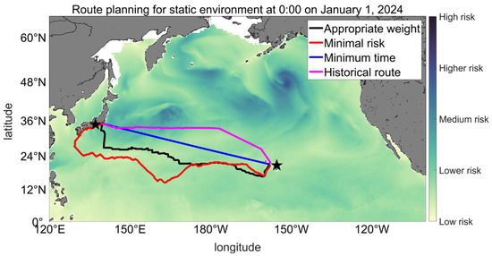
Figure 9.
Different types of track planning.
As can be seen from Figure 9, when the weight risk of the selected objective function is at least 1, the entire route is in the low-risk area. However, it is obvious that the range is longer and some routes are also close to the coastline, which is not practical in general. When only the flight time is considered, the entire route also passes through a large risk area, and some routes violate the hard safety restrictions. Historical routes give an average of the six actual routes, which have a shorter range. However, some routes are in the medium-risk area, and some areas also violate the safety guidelines. Various values of different routes are shown in Table 3:
Table 3.
Table of various values for different voyages.
As can be seen from the table, through calculation, the average risk value of the route with the least risk is 0.14; the average VAR of historical routes is 0.26; the risk value of the appropriately weighted route is 0.14; and the minimum time risk value is 0.20. The sailing time of the least risk route is 338.7388 h; the sailing time of the appropriately weighted route is 266.4724 h. The voyage time decreased by 72.2664 h. The voyage time decreased significantly, but the total risk value did not increase significantly. The wind and waves faced by the shortest time and historical routes will be large in some areas, and the maximum risk will reach about 0.5. In general, the average risk of the four routes is not very high, but the sailing time varies greatly. Given the appropriate weight, the planned route can reduce both the navigation risk and the navigation time, which proves the effectiveness of the model. In actual application, the weights of the three objective functions derive not only from the Pareto-optimal trade-offs among objectives under multi-objective planning, but also from the decision-maker’s preferences or practical requirements. For instance, in benign overall conditions, greater emphasis may be placed on reducing sailing time, whereas if the vessel’s risk-resistance capability is limited, navigational safety must be given top priority. Consequently, the weights of the three objective functions are adapted to the prevailing circumstances. In this paper, navigation safety is treated as the primary objective. From the Pareto-optimal set obtained through multi-objective planning, we selected the weight combination that yields only a slight increase in overall route risk compared with a risk-only solution while achieving a substantial reduction in sailing time: a navigation risk of 0.7, a sailing time of 0.2, and a water depth of 0.1.
However, the route depicted in Figure 9 is based on a static environment at a single time point. Since the navigation time for the appropriately weighted route is 266.4724 h, the route design should be adjusted according to environmental changes over time. Therefore, this section uses a 24 h interval. By collecting meteorological and oceanographic data at different time points over 24 h, the average environmental data is calculated to determine the risk value. The data undergoes a daily averaging process with a 24 h cycle (starting daily at UTC 00:00), where each cycle comprises 24 equally spaced measurements (sampling frequency: 1 per hour). Due to the difficulty of obtaining measured data, this paper only employs processed historical actual data for simulation. In practical application, the model can, during navigation, adopt forecast data to replan the global route every twelve hours or at shorter intervals, continuously updating the route. Routes are then planned based on the risk values for different time periods, as shown in Figure 10:
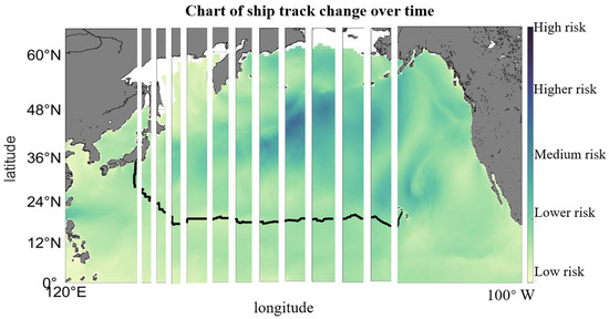
Figure 10.
Dynamic optimization diagram of flight track.
5.2. Field of Ship Safety
Zhou et al. [40] conducted research using principal component analysis and rough set-based methods, revealing significant differences in the degree of influence of various factors on ship domains. Factors with greater influence include the encounter angle between ships, regional ship density, crew quality, ship speed, ship length, and ship type, while factors with lesser influence include wind, waves, currents, and visibility. Results from the rough set-based method indicate that environmental factors such as wind, waves, and currents have a negligible impact, and their importance is also very low in the principal component analysis. Overall, the encounter relationship between ships has the greatest impact on the ship domain, followed by human factors and basic ship parameters, while the influence of meteorological and oceanographic conditions is minimal.
The ships in the formation studied in this paper give an ideal meeting relation. The marine environment factors change with time and space. Taking a 50,000-ton container ship as an example, three kinds of ship safety fields with different crew qualities are given. Figure 11 shows the following:
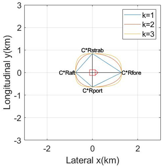
Figure 11.
Ship domain model diagram.
In order to ensure the safety of the ship’s navigation, when the obstacle touches the ship’s safety field, the ship will turn on the obstacle avoidance function to avoid the obstacle. Moreover, the safety domains of ships within the fleet must not overlap, which necessitates maintaining a safe distance between ships to ensure the stability of the fleet’s formation during navigation.
5.3. Ship Obstacle Avoidance Function
Based on the basic idea of the artificial potential field algorithm and the improvement of defects, the realization of the ship obstacle avoidance function is simulated. It is assumed that there are multiple obstacles between two grid points in the global path planning of a fleet of following ships. The ship needs to return to the formation after avoiding obstacles. The initial stage and avoidance route are shown in Figure 12 and Figure 13:
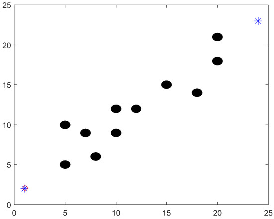
Figure 12.
The initial stage of the ship avoiding obstacles.
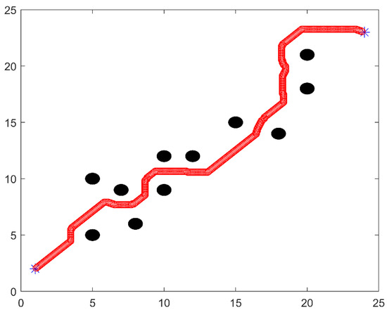
Figure 13.
Route map of ship avoiding obstacles.
As can be seen from Figure 13, from the initial point to the target point (Indicated by blue asterisks in the figure), the ship basically begins to evade when it is a certain distance away from the obstacle. Sail in a straight line when there are no obstacles nearby. The model basically meets the requirements.
5.4. Function of Stable Structure of Ship Formation
Ships are distributed in different locations during the initial phase. The leading ships sail along the grid points of the global track planning, and the rest follow the ships to gradually reach the predetermined formation structure and maintain stability during the voyage. Select the initial route from 00:00 to 12:00 on 1 January 2024 using global planning, as shown in Figure 14:
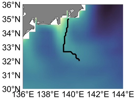
Figure 14.
Excerpts of global track planning routes.
The course of each iteration of the leader of the ship formation in this section is shown in Figure 14. When the whole formation does not reach the established structure, the grid iteration speed of the leader decreases. After the stable structure is reached, the pilot iterates the predetermined grid points at normal speed. Due to the large spacing of the grid points, the grid points are refined by interpolation to enhance the authenticity of the simulation. The rest of the following ships use the leader-following model to maintain stable formation navigation, and the specific results are shown in Figure 15:
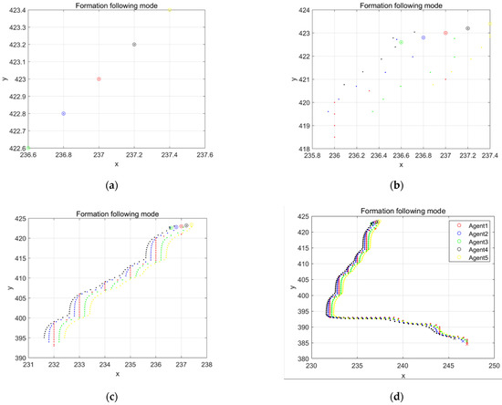
Figure 15.
Simulation diagram of ship formation leadership following.
As shown in Figure 15, the red routes represent the leaders. The remaining routes represent followers. In order to make the change process clearer, the drawing results reduce the distance of the A* planning grid points and enlarge the details of the follower changes. Figure 15a,b shows the formation process from the initial stage to the formation of a stable formation structure. The initial phase moves from the initial position to the designated position before following the lead ship forward. Figure 15c,d show the stabilization phase. In the general direction, the whole ship formation moves completely in accordance with the route planned by the A* algorithm. Each ship can basically form a stable formation structure to move forward.
6. Conclusions
An improved A algorithm is proposed for optimal route selection in long-distance ship transportation, supplemented by two local planning methods to ensure safe navigation for fleets. The algorithm enhances the original A algorithm by incorporating multiple cost options into the actual cost function and heuristic cost function, while imposing safety constraints to optimize routes and ensure ship safety. The model is validated through multi-objective optimization of routes for actual container ships under different cost considerations. The improved A* algorithm demonstrates strong performance across various cost factors, allowing different results by adjusting weights while prioritizing ship safety. For the entire fleet, local planning complements the global route optimization. First, a ship safety domain is established, providing a basis for obstacle avoidance and maintaining fleet structure stability. Each ship’s obstacle avoidance ensures individual safety, while the stable fleet structure enhances overall safety, improves navigation efficiency, and facilitates communication, navigation, and positioning.
Additionally, taking a 50,000-ton container ship with constraints as an example, the primary objective functions are minimizing risk and the shortest time from the departure point to the destination, with sufficient ocean depth as a secondary condition. Furthermore, two IMO safety criteria—speed limits and resonance period restrictions—are added to ensure dynamic safety. By adjusting the weights of the objective functions, three different routes are obtained: shortest time, minimum risk, and balanced weight. These are compared with the average of historical routes in the North Pacific. The minimum risk route has an average risk value of 0.14, the historical route averages 0.26, the appropriate weight route has a risk value of 0.16, and the shortest time route has a risk value of 0.20. The minimum risk route takes 338.7388 h, while the balanced weight route takes 266.4724 h, reducing navigation time by 72.2664 h significantly without a notable increase in total risk. In contrast, the shortest time and historical routes face higher wind and wave risks in some areas, with maximum risk values reaching around 0.5. Additionally, routes are planned for twelve days under dynamic environmental conditions. The overall results demonstrate the advantages of the proposed algorithm, providing more reliable options for practical navigation.
To ensure fleet safety, local planning is added to supplement the overall global planning. Based on ship parameters, meteorological and oceanographic conditions, and crew quality, safety domains between ships and between ships and obstacles are defined, which must not be violated during obstacle avoidance and fleet formation. The shortcomings of the artificial potential field method are addressed by integrating globally planned routes to achieve obstacle avoidance for each vessel. Using the artificial potential field and leader–follower approach, the fleet’s ships gradually form and maintain the predetermined structure from their initial positions. Simulation results suggest the potential effectiveness of the proposed algorithm, with its practical performance requiring future sea trial validation, while simulations may contribute to it and suggest improvements. Subsequent work will cooperate with the relevant maritime authorities to conduct practical validation of the model. In future research, we will focus on improving the model impact formulas for multi-constrained ship weather route optimization in the A algorithm and incorporating the influence of additional environmental factors. For example, Maritime low visibility poses significant challenges to the safety of vessel fleet navigation. Reduced visibility impairs ship maneuverability and heightens risks of collisions and real-time tracking failures [41]. Anomalous ocean currents may induce vessel drift, posing significant dragging anchor risks, especially for anchored fleets. Such currents can trigger mutual collisions among vessels within the fleet in confined and complex waters. When a vessel moves relative to surrounding currents, hydrodynamic pressure forces act upon the hull [42,43]. Excessively high sea surface temperatures (SST) may cause main engine overheating, necessitating enhanced cooling or speed reduction. Conversely, abnormally low SST can lead to sea ice formation, posing severe threats to navigation safety [44]. More complex and realistic meteorological and oceanographic models tailored to ship safety will be integrated into the algorithm, while considering additional objectives such as economic efficiency and environmental sustainability. Additionally, the relative merits of different algorithms must be considered; therefore, we will combine global and local planners in various ways and conduct comparative simulations under identical or extreme conditions, evaluating path optimality, computational efficiency, trajectory smoothness, safety-risk indices, and energy economy to select the superior approach. Furthermore, fleet research will be better integrated into global route planning, enabling comprehensive consideration in overall planning. The goal is to develop a high-precision, high-performance, and high-efficiency three-dimensional ship path optimization method suitable for more complex scenarios.
Author Contributions
Conceptualization, M.H. and Z.G.; methodology, Z.G.; validation, Z.G., H.L.; formal analysis, Z.G.; investigation, Z.G. and M.H.; data curation, Z.G.; writing—original draft preparation, Z.G.; writing—review and editing, M.H., Y.L., Y.Z. and L.Q.; visualization, Z.G.; supervision, M.H., Y.L., Y.Z. and L.Q.; project administration, M.H.; funding acquisition, M.H. All authors have read and agreed to the published version of the manuscript.
Funding
This work was supported by the Natural Science Foundation of Hunan Province, project number 2023JJ10054, and the National Natural Science Foundation of China, project number 41875061.
Data Availability Statement
The data presented in this study are available in [Global Ocean Physics Analysis and Forecast] at [https://doi.org/10.48670/moi-00016]. These data were derived from the following resources available in the public domain: [Copernicus Marine Data Store and https://data.marine.copernicus.eu/products?q=wave (accessed on 27 January 2025)]. The data presented in this study are available in [ERA5 hourly data on single levels from 1940 to present] at [https://doi.org/10.24381/cds.adbb2d47 (accessed on 27 January 2025)]. These data were derived from the following resources available in the public domain: [Climate Data Store and https://cds.climate.copernicus.eu/datasets (accessed on 27 January 2025)].
Conflicts of Interest
The authors declare that they have no known competing financial interests or personal relationships that could have appeared to influence the work reported in this paper.
References
- Lu, L.F.; Sasa, K.; Sasaki, W.; Terada, D.; Kano, T.; Mizojiri, T. Rough wave simulation and validation using onboard ship motion data in the southern hemisphere to enhance ship weather routing. Ocean Eng. 2017, 144, 61–77. [Google Scholar] [CrossRef]
- Zhang, G.; Cao, Q.; Huang, C.; Zhang, X. Adaptive neural quantized formation control for heterogeneous underactuated ships with the MVS guidance. Ocean. Eng. 2024, 294, 116760. [Google Scholar] [CrossRef]
- Du, W. Route Optimization of Ocean-Going Ships with Time-Distance-Weather Coupling. Ph.D. Thesis, Harbin Engineering University, Harbin, China, 2023. [Google Scholar]
- Du, W.; Li, Y.; Zhang, G.L.; Wang, C.; Zhu, B.; Qiao, J. Ship weather routing optimization based on improved fractional order particle swarm optimization. Ocean Eng. 2022, 248, 110680. [Google Scholar] [CrossRef]
- Saad, M.; Salameh, A.I.; Abdallah, S.; El-Moursy, A.; Cheng, C.T. A Composite Metric Routing Approach for Energy-Efficient Shortest Path Planning on Natural Terrains. Appl. Sci. 2021, 11, 6939. [Google Scholar] [CrossRef]
- Zhang, X. Simulation of maneuverability of large container ships under wind and waves. Ship Sci. Technol. 2022, 44, 149–152. [Google Scholar]
- Niu, H.L.; Ji, Z.; Savvaris, A.; Tsourdos, A. Energy efficient path planning for Unmanned Surface Vehicle in spatially-temporally variant environment. Ocean Eng. 2020, 196, 106766. [Google Scholar] [CrossRef]
- Chen, X.; Bose, N.; Brito, M.; Khan, F.; Millar, G.; Bulger, C.; Zou, T. Risk-based path planning for autonomous underwater vehicles in an oil spill environment. Ocean Eng. 2022, 266, 113077. [Google Scholar] [CrossRef]
- Tong, X.L.; Yu, S.N.; Liu, G.Y.; Niu, X.D.; Xia, C.J.; Chen, J.K.; Yang, Z.; Sun, Y.Y. A hybrid formation path planning based on A* and multi-target improved artificial potential field algorithm in the 2D random environments. Adv. Eng. Inform. 2022, 54, 101755. [Google Scholar] [CrossRef]
- Wang, L.P.; Zhang, Z.; Zhu, Q.D.; Ma, S. Ship Route Planning Based on Double-Cycling Genetic Algorithm Considering Ship Maneuverability Constraint. IEEE Access 2020, 8, 190746–190759. [Google Scholar] [CrossRef]
- Lu, W.; Wu, M.G. Optimization of vehicle automatic navigation path based on remote sensing and GIS. Opt. Int. J. Light Electron. Opt. 2022, 270, 169952. [Google Scholar] [CrossRef]
- Wang, H.B.; Li, X.G.; Li, P.F.; Veremey, E.I.; Sotnikova, M.V. Application of Real-Coded Genetic Algorithm in Ship Weather Routing. J. Navig. 2018, 71, 989–1010. [Google Scholar] [CrossRef]
- Krell, E.; King, S.A.; Garcia, C.L.R. Autonomous Surface Vehicle energy-efficient and reward-based path planning using Particle Swarm Optimization and Visibility Graphs. Appl. Ocean Res. 2022, 122, 103125. [Google Scholar] [CrossRef]
- Zhong, J.B.; Li, B.Y.; Li, S.X.; Yang, F.R.; Li, P.H.; Cui, Y. Particle swarm optimization with orientation angle-based grouping for practical unmanned surface vehicle path planning. Appl. Ocean Res. 2021, 111, 102658. [Google Scholar] [CrossRef]
- Serani, A.; Fasano, G.; Liuzzi, G.; Lucidi, S.; Iemma, U.; Campana, E.F.; Stern, F.; Diez, M. Ship hydrodynamic optimization by local hybridization of deterministic derivative-free global algorithms. Appl. Ocean Res. 2016, 59, 115–128. [Google Scholar] [CrossRef]
- Zhang, G.Y.; Wang, H.B.; Zhao, W.; Guan, Z.Y.; Li, P.F. Application of Improved Multi-Objective Ant Colony Optimization Algorithm in Ship Weather Routing. J. Ocean Univ. China 2021, 20, 45–55. [Google Scholar] [CrossRef]
- Öztürk, Ü.; Akdağ; M.; Ayabakan, T. A review of path planning algorithms in maritime autonomous surface ships: Navigation safety perspective. Ocean Eng. 2022, 251, 111010. [Google Scholar] [CrossRef]
- Guan, Z.Y.; Wang, Y.; Zhou, Z.; Wang, H.B. Research on early warning of ship danger based on composition fuzzy inference. J. Mar. Sci. Eng. 2020, 8, 1002. [Google Scholar] [CrossRef]
- Shang, M.; Chu, M.; Grethler, M. Path Planning Based on Artificial Potential Field and Fuzzy Control. In Proceedings of the 2020 International Conference on Intelligent Computing, Automation and Systems (ICICAS), Chongqing, China, 11–13 December 2020; pp. 304–308. [Google Scholar]
- Yang, X. Development of Obstacle Avoidance for Autonomous Vehicles and an Optimization Scheme for the Artificial Potential Field Method. In Proceedings of the 2nd International Conference on Computing and Data Science, Stanford, CA, USA, 28–29 January 2021. [Google Scholar]
- Zhou, X.; Xu, R.; Cheng, G. AUV Path Planning in Dynamic Environment Based on Improved Artificial Potential Field Method Based on Visibility Graph. J. Phys. Conf. Ser. 2022, 2383, 012090. [Google Scholar]
- Liu, L.; Wang, B.; Xu, H. Research on Path-Planning Algorithm Integrating Optimization A-Star Algorithm and Artificial Potential Field Method. Electronics 2022, 11, 3660. [Google Scholar] [CrossRef]
- Zhang, M.; Montewka, J.; Manderbacka, T.; Kujala, P.; Hirdaris, S. A big data analytics method for the evaluation of ship—Ship collision risk reflecting hydrometeorological conditions. Reliab. Eng. Syst. Saf. 2021, 213, 107674. [Google Scholar] [CrossRef]
- Wang, J.; Wang, R.; Lu, D.H.; Zhou, H.; Tao, T.Y. USV Dynamic Accurate Obstacle Avoidance Based on Improved Velocity Obstacle Method. Electronics 2022, 11, 2720. [Google Scholar] [CrossRef]
- Xu, T.Y.; Zhang, S.Q.; Jiang, Z.Y.; Liu, Z.C.; Cheng, H. Collision Avoidance of High-Speed Obstacles for Mobile Robots via Maximum-Speed Aware Velocity Obstacle Method. IEEE Access 2020, 8, 138493–138507. [Google Scholar] [CrossRef]
- Ding, L.; Guo, G. A backstepping method for fleet formation control. Control. Decis. 2012, 27, 299–303. [Google Scholar]
- Liu, B.; Chu, T.; Wang, T.; Xie, G. Controllability of a leader–follower dynamic network with switching topology. IEEE Trans. Autom. Control 2008, 53, 1009–1013. [Google Scholar] [CrossRef]
- Arcak, M.; Fossen, T.; Ihle, I. Passivity-based designs for synchronized path-following. Automatica 2007, 43, 1508–1518. [Google Scholar] [CrossRef]
- Huang, F.J.; Wu, P.; Li, X.X. Distributed Flocking Control of Quad-rotor UAVs with Obstacle Avoidance Under the Parallel-triggered Scheme. Int. J. Control. Autom. Syst. 2021, 19, 1375–1383. [Google Scholar] [CrossRef]
- Ihle, I.F.; Jouffroy, J.; Fossen, T.I. Formation Control of Marine Surface Craft: A Lagrangian Approach. IEEE J. Ocean. Eng. 2006, 31, 922–934. [Google Scholar] [CrossRef]
- Sun, G.B.; Zhou, R.; Di, B.; Hu, Y. A physicochemically inspired approach to flocking control of multiagent system. Nonlinear Dyn. 2020, 102, 2627–2648. [Google Scholar] [CrossRef]
- Zhang, W.Y.; Xia, D.W.; Chang, G.Y.; Hu, Y.; Huo, Y.J.; Feng, F.Y.; Li, Y.T.; Li, H.Q. APFD: An effective approach to taxi route recommendation with mobile trajectory big data. Front. Inf. Electron. Eng. 2022, 23, 1494–1510. [Google Scholar] [CrossRef]
- Liu, F. Study on ship stall in wind and waves. J. Dalian Marit. Univ. 1992, 4, 347–351. [Google Scholar]
- Wang, F.W.; Jia, C.Y. Study on ship’s preferred route. J. Dalian Marit. Univ. 1998, 2, 62–65. [Google Scholar]
- Svec, P.; Schwartz, M.; Thakur, A.; Gupta, S.K. Trajectory planning with look-ahead for Unmanned Sea Surface Vehicles to handle environmental disturbances. In Proceedings of the IEEE/RSJ International Conference on Intelligent Robotics and Systems (IROS 2011), San Francisco, CA, USA, 25–30 September 2021; pp. 1154–1159. [Google Scholar]
- Fujii, Y.; Tanaka, K. Traffic Capacity. J. Navig. 1971, 24, 543–552. [Google Scholar] [CrossRef]
- Szlapczynski, R.; Szlapczynska, J. Review of ship safety domains: Models and applications. Ocean Eng. 2017, 145, 277–289. [Google Scholar] [CrossRef]
- Wang, N. A novel analytical framework for dynamic quaternion ship domains. J. Navig. 2013, 66, 265–281. [Google Scholar] [CrossRef]
- Manel, G.; Clara, B.; Marcella, C.S. A comprehensive ship weather routing system using CMEMS products and A* algorithm. Ocean Eng. 2022, 255, 111427. [Google Scholar] [CrossRef]
- Zhou, D.; Zheng, Z.Y. Analysis on the importance of factors affecting ship field when visibility is good. J. Harbin Eng. Univ. 2017, 38, 20–24. [Google Scholar]
- Liu, H.; Xu, X.; Chen, X.; Li, C.; Wang, M. Real-Time Ship Tracking under Challenges of Scale Variation and Different Visibility Weather Conditions. J. Mar. Sci. Eng. 2022, 10, 444. [Google Scholar] [CrossRef]
- Pan, W.; Xie, X.-L.; He, P.; Bao, T.-T.; Li, M. An automatic route design algorithm for intelligent ships based on a novel environment modeling method. Ocean Eng. 2021, 237, 109603. [Google Scholar] [CrossRef]
- Wu, W.P.; Gunnu, G.R.S. Positioning capability of anchor handling vessels in deep water during anchor deployment. J. Mar. Sci. Technol. 2015, 20, 487–504. [Google Scholar] [CrossRef][Green Version]
- Liu, C.; Hu, S.; Li, P.C.; Qian, T.; Yuan, Y.; Wen, H.; Zhang, D. Impact mechanism and prediction methods of harsh environmental factors on typical wave-induced icing during polar ship navigation. Ocean Eng. 2025, 321, 120409. [Google Scholar] [CrossRef]
Disclaimer/Publisher’s Note: The statements, opinions and data contained in all publications are solely those of the individual author(s) and contributor(s) and not of MDPI and/or the editor(s). MDPI and/or the editor(s) disclaim responsibility for any injury to people or property resulting from any ideas, methods, instructions or products referred to in the content. |
© 2025 by the authors. Licensee MDPI, Basel, Switzerland. This article is an open access article distributed under the terms and conditions of the Creative Commons Attribution (CC BY) license (https://creativecommons.org/licenses/by/4.0/).