Machine Learning-Based Recursive Prediction and Application of Green’s Function of Water-Wave Radiation and Diffraction

Abstract

The frequency-domain free-surface Green’s function method is widely used in solving ship hydrodynamic problems, with its core challenge lying in the computation of the Green’s function and its partial derivatives. This study analyzes the relationship between the free-surface Green’s function and its derivatives, proposing a machine learning-based recursive prediction method termed the pulsating source recursive prediction method. The accuracy and efficiency of this method under various parameter settings are investigated, and its application to the hydrodynamic calculations of container ship S175 and a bulk carrier is demonstrated. Results show that the predicted Green’s function achieves an accuracy of 3–6 decimals, with computational efficiency surpassing numerical methods and matching analytical approaches. The hydrodynamic results are reliable, confirming the method’s practical value.

1. Introduction

Within the framework of potential flow theory, the Green’s function method is often employed to calculate the hydrodynamic performance of ships. Also known as the singularity distribution method, the Green’s function method reduces computational complexity and improves efficiency by distributing sources and sinks on the flow field boundaries and discretizing integral equations onto these boundaries [1,2]. In three-dimensional potential flow theory, the Green’s function method includes the simple Green’s function method and the complex Green’s function method. The former has a straightforward mathematical formulation and is easier to handle but requires a larger mesh discretization on free surfaces. The latter, also called the free-surface Green’s function method, eliminates the need to discretize the free surface. However, the computation of the free-surface Green’s function itself and its partial derivatives is more complex, representing a key challenge. The accuracy and efficiency of these calculations directly impact the results of hydrodynamic performance analysis. Regarding the computation of the frequency-domain infinite-depth zero-speed free-surface Green’s function, numerous scholars have conducted extensive research.

In 1982, Noblesse [3] proposed the concepts of near-field and far-field terms and provided corresponding expressions, using asymptotic expansion series and convergent series methods for calculation. In 1984, Newman [4] expressed the zero-speed pulsation Green’s function and its partial derivatives as the sums of finite integrals, Bessel functions, and Struve functions and used Romberg integration for numerical solution. Later, to achieve better prediction efficiency, in 1985 [5], a series expansion method with an accuracy of 10⁻⁶ was proposed, and in 1992 [6], the Chebyshev approximation method was introduced. This method treated the Green’s function as the sum of a simple but highly oscillatory analytical part and a slowly varying residual function, dividing the computational domain into different subregions and using Chebyshev polynomials to approximate the residual function, achieving an accuracy of 10⁻⁵. Guided by this research approach, scholars such as Wang [7], Zhou et al. [8], and Duan et al. [9] conducted a series of studies on the residual functions of the Green’s function and its partial derivatives. In 2009, Yao [10] introduced Gaussian integration into the calculation of the Green’s function, achieving an accuracy of 10⁻⁶. In 2017, Wu [11] expressed the Green’s function and its derivatives as the sum of fundamental spatial singularities, non-oscillatory near-field terms, and wave terms, using only real variables and basic elementary functions to achieve global polynomial fitting for the near-field terms. This method achieved an accuracy of 10⁻³ and exhibited excellent computational efficiency. In 2019, Shan et al. [12] improved Newman’s subregion division method and proposed an optimized Chebyshev approximation method, achieving an accuracy of 10⁻⁹. In 2020, Chang et al. [13] applied machine learning concepts to the calculation of the pulsating source Green’s function, providing a new approach for computing the Green’s function and its derivatives, with an accuracy of 10⁻⁴. However, its computational efficiency shows no advantage compared to analytical approximation methods. It is worth mentioning that the author of this paper, Renchuan Zhu, supervised the work in references [12,13], and this paper is a continuation and refinement of the previous work. By analyzing the relationship between the free-surface Green’s function and its derivatives, this paper proposes a machine learning-based recursive prediction method termed the pulsating source recursive prediction method, which significantly improves computational efficiency.

This paper addresses the computational problem of the frequency-domain infinite water depth zero-speed free-surface Green’s function. By exploring the correspondence between the free-surface Green’s function and its partial derivatives, a machine learning-based recursive prediction method for the Green’s function and its partial derivatives is proposed, termed the pulsating source recursive prediction method. The neural network training is completed in Matlab 2022a software, and after extracting the network parameters, a numerical calculation program code is written in Fortran 2019 to explore the computational accuracy and efficiency of the method under different parameter settings. Fortran has a recognized advantage in the field of high-performance scientific computing, offering high computational efficiency and numerical stability. As a traditional language for scientific computing, Fortran can more directly reflect the performance characteristics of algorithms themselves, avoiding interference introduced by differences in language features. The container ship S175 and a bulk carrier are selected as the validation objects for the method’s application. The pulsating source recursive prediction method is applied to calculate the motion response, wave diffraction forces, and hydrodynamic coefficients of the two ships, and the results are compared with those obtained by the three-dimensional pulsating source speed correction method (Romberg integration method) to verify the application effectiveness of the proposed method.

2. Theory of Green’s Function

2.1. Green’s Function Solution for Radiation Potential

For a ship undergoing harmonic oscillations, the normalized velocity potential of the ship six-degree-of-freedom motion ${\varphi }_j(x,y,z)$ satisfies

$$\left.\begin{array}{l}{\nabla }^2{\varphi }_j(x,y,z)=0\\ {\displaystyle \frac{\partial {\varphi }_j}{\partial z}}-k{\varphi }_j=0\\ {\left.{\displaystyle \frac{\partial {\varphi }_j}{\partial n}}\right|}_{S_0}=-i\omega {\displaystyle \sum _{j=1}^6{x}_j}{\tilde{n}}_j\\ {\left.{\displaystyle \frac{\partial {\varphi }_j}{\partial z}}\right|}_{z=-H}=0\\ \underset{R_0\to \infty }{\lim }\sqrt{R_0}\left[{\displaystyle \frac{\partial {\varphi }_j}{\partial R_0}}-ik{\varphi }_j\right]=0\\ \end{array}\right\}$$

(1)

where ϕ_j is the normalized velocity potential corresponding to the motion mode j, where j = 1, 2, 3, 4, 5, 6 represent surge, sway, heave, roll, pitch, and yaw, respectively. R₀ = $\sqrt{x^2+y^2}$ denotes the horizontal distance from the field point to the source point. In infinite water depth, wave number k = ω²/g. The boundary conditions, listed from top to bottom, are the fluid continuity principle, free-surface condition, body-surface condition, seabed condition, and far field radiation condition.

The velocity potential is solved using the free-surface Green’s function method, which only requires discretizing the mean wetted hull surface S₀. That is, the velocity potential at any point P(x, y, z) within the domain can be expressed as

$${\varphi }_j(P)=-{\displaystyle \frac{1}{4\pi }}{\displaystyle {\iint }_{S_0}\left[{\varphi }_j(Q)\frac{\partial G(P,Q)}{\partial n}-G\frac{\partial {\varphi }_j}{\partial n}\right]}dS$$

(2)

where the Green’s function G(P, Q) satisfying the linear free-surface condition is only related to the positions of the source and field points, and its specific expression is given in Section 2.2.

After discretizing the hull surface using the panel method to obtain the velocity potential, the hydrodynamic coefficients can be calculated via Equation (3) [1,2]:

$${\mu }_{jk}+i{\displaystyle \frac{{\lambda }_{jk}}{\omega }}=\rho {\displaystyle {\iint }_{S_0}{\varphi }_k\frac{\partial {\varphi }_j}{\partial n}dS}$$

(3)

where the subscript k represents the motion mode number, j denotes the direction of the force/moment (j = 1–3 for forces, and j = 4–6 for moments), and μ_jk, λ_jk are referred to as the added mass and damping coefficient, respectively.

2.2. Frequency-Domain Green’s Function

The frequency-domain free-surface Green’s function method plays a crucial role in analyzing hydrodynamic interactions for ships and offshore structures. At its core, this method relies on accurately computing the free-surface Green’s function and its partial derivatives. Denote the field point coordinates as P(x, y, z) and the source point coordinates as Q(ξ, η, ζ). The infinite water depth zero-speed frequency-domain free-surface Green’s function, as shown in Equation (2), can be expressed as follows:

$$G(P,Q)=1/r+1/r_1+kF(X,Y)+2\pi ik{e}^{-Y}{J}_0(X)$$

(4)

where k = ω_e²/g (ω_e is the encounter wave frequency), $R=\sqrt{{(x-\xi )}^2+{(y-\eta )}^2}$, $r=\sqrt{R^2+{(z-\zeta )}^2}$, and $r_1=\sqrt{R^2+{(z+\zeta )}^2}$, X = kR, Y = −k (z + ζ).

In the above equation, the numerical solution 1/r + 1/r₁ and 2πike^−YJ₀(X) is easy to implement, so the key to solving lies in calculating the fluctuating part F(X, Y). According to Newman’s research [4], F(X, Y) is expressed as

$$F(X,Y)=-2e^{-Y}{\displaystyle {\int }_0^Y{e}^t{(X^2+t^2)}^{-1/2}dt-\pi e^{-Y}}[Y_0(X)+H_0(X)]$$

(5)

By taking the partial derivatives of F in the horizontal direction X and the vertical direction Y, it can be obtained:

$$F_X(X,Y)=\partial F(X,Y)/\partial X=-2e^{-Y}+\pi e^{-Y}[H_1(X)+Y_1(X)]+2X{\displaystyle {\int }_0^Y{e}^t{(X^2+t^2)}^{-3/2}{e}^{t-Y}dt}$$

(6)

$$F_Y(X,Y)=\partial F(X,Y)/\partial Y=-{\displaystyle \frac{2}{R_1}}-F$$

(7)

where Y_n (⋅) is the Bessel function of the second kind of order n, H_n (⋅) is the Struve function of order n, and R₁ =$\sqrt{X^2+Y^2}$.

Continuing to find the partial derivative of F_X in the vertical direction Y, it can be obtained:

$$F_{XY}=2X{(X^2+Y^2)}^{-3/2}-F_X$$

(8)

According to the above calculation formula, it can be found that there is an easily handled mutual calculation relationship between F and F_Y, and a similar relationship also exists between F_X and F_XY. To meet the requirements of hydrodynamic calculations, it is necessary to solve the problem of efficiently calculating F and F_Y.

3. Recursive Prediction Method and Machine Learning

3.1. Recursive Prediction Method

Based on the theory outlined in Section 2.2, this paper introduces a recursive prediction method to calculate the free-surface Green’s function with high efficiency and precision. The specific principle is as follows.

Usually, we have the approximation of the first-order Taylor expansion of a single-variable function f(Y) near the point Y₀:

$$f(Y)=f(Y_0)+{\left.\frac{\partial f}{\partial Y}\right|}_{Y=Y_0}(Y-Y_0)+o(Y-Y_0)$$

(9)

This relational expression is applied to the solution process of F and F_X mentioned in Section 2.2. The high-order terms on the right-hand side of Equation (9) are neglected as an approximation, considering Y as the single variable; thereby, the approximate relationship between F and F_Y is established:

$$F(X,Y_0+\Delta Y)=F(X,Y_0)+F_Y(X,Y_0)\cdot \Delta Y$$

(10)

where ΔY = Y − Y₀. Similarly, an approximate relationship is also established between F_X and F_XY:

$$F_X(X,Y_0+\Delta Y)=F_X(X,Y_0)+F_{XY}(X,Y_0)\cdot \Delta Y$$

(11)

According to Equation (10), if an appropriate ΔY can be selected, the value of F(X, Y₀ + ΔY) at the point (X, Y₀ + ΔY) can be calculated based on the values of F(X, Y₀) and F_Y(X, Y₀) at the current point (X, Y₀). Then, the value of F_Y(X, Y₀ + ΔY) can be computed by Equation (7). By repeating this process and iterating forward step by step, the value of F(X, Y₀ + nΔY) can be calculated, with n representing the number of repetitions in the recursive calculation. The prediction of F_X(X, Y) follows a similar approach. This technique and process are referred to as the recursive prediction method in this paper.

Regard X as a variable in Equations (10) and (11); if there are the values of F and F_X on one straight line with fixed Y₀, then F and F_X in the whole domain can be obtained by using the recursive prediction method. To reduce the loss of precision in calculating F(X, Y) during the recursive process, it is necessary to arrange F(X, Y) on some straight recursive lines as the datum lines where Y is fixed. For example, totally, there are 20 straight datum lines in the whole domain with fixed Y₀, Y₁, …,Y₂₀.

In the present research, the neural network method is employed to train the function F(X, Y) varying with X on each datum line. The obtained neural network models of F(X, Y) on datum lines with different fixed Y will be saved for future calls. Thus, in practical recursive process, first identify the datum line which the forecast point (X^′, Y^′) nearest to, for example, the n-th datum line is, and then, one can substitute the value of X^′ into the neural network model corresponding to the n-th datum line to calculate the value of F(X^′, Y_n); then, using the chosen small step length ΔY, perform several times of recursive calculation process from F(X^′, Y_n), and finally one can obtain the value of F(X^′, Y^′).

3.2. Neural Network Model of Function F and F_X on Datum Line in Machine Learning

The principles of neural networks have been widely popularized and will not be repeated here. For detailed derivations, please refer to [14]. Taking a simple three-layer neural network as an example, its structure is shown in Figure 1 below, including the input layer, hidden layer, and output layer.

In the structural diagram of a neural network, ξ = [ξ₁, ξ₂, …, ξ_m] is a one-dimensional to multi-dimensional matrix, representing the input values of the network; γ is the output value of the network. w is the synaptic weight, b is the bias, and the composition of its matrix depends on the number of hidden layers and nodes. σ is the activation function, and common types of activation functions are detailed in [15]. The relationship between the input and output values can be expressed as

$$\gamma =\sigma \left({\displaystyle \sum _{i=1}^m{w}_i{\xi }_i+b}\right)$$

(12)

With the preset network structure and activation function, once the values of w and b in the hidden layer are extracted from the trained neural network, the value of γ can be calculated based on the input value of ξ_i according to Equation (12). In fact, the training process also involves normalization and denormalization, which should also be reflected in the program reproduction.

The establishment logic of the entire prediction model is as follows: training of high-precision database → extraction of neural network parameters → reproduction of prediction model → γ_pre = f_net(ξ_inp).

First, the “training sample set density”, “neural network complexity”, and “single datum line recursive prediction coverage range“ in machine learning are investigated.

(1)

The training sample set density

Three sets of training sample datasets were established with densities of 0.1, 0.05, and 0.01. After the training was completed, the models built using different training sample datasets were applied to test samples with a density of 0.01, and the training error conditions of the different models were compared.

The results show that the forecast error condition performs better with the increase of training sample set density, but as the training sample set density gradually increases, this effect becomes weaker. If the training sample set density is set to 0.1, the forecast error is relatively larger; while when the training sample set density is 0.05, 0.01, or 0.005, the overall forecast error conditions are quite similar. Considering that when the training sample set density is too small, the neural network is prone to fall into local optima, and a larger training sample set density increases training time, a balanced approach suggests selecting a training sample set density of 0.01 for subsequent steps.

(2)

The neural network complexity

Considering that when Y is small (i.e., near the free surface), the value and fluctuations of F(X, Y) are relatively large, while when Y is large (i.e., at greater depths), the value and fluctuations of F(X, Y) are relatively small. When applying the same network structure settings for model training and F(X, Y) prediction in different regions, the overall prediction error tends to improve as Y increases. In practice, the network settings should be adjusted according to the characteristics of different regions. For example, a more complex network should be used near the free surface, while a simpler network can be employed at greater depths.

Recursive forecasting is conducted at different Y values with varying numbers of nodes. The results show that the forecasting error improves as the number of network nodes increases, but the improvement has its limits. Under fixed other conditions, once the number of network nodes reaches a certain level, it no longer has a significant impact on the forecasting error. Additionally, by comparing values at different Y positions, it can be observed that in regions with smaller Y values, the forecast error performance is average, requiring more network nodes to be set—in other words, achieving sufficient forecast accuracy by configuring a more complex network. In regions with larger Y values, the forecast error performance is good. Considering that setting more network nodes would consume additional time for relatively complex network forecasts, in regions with better forecast error performance, a lower-complexity network can be considered, sacrificing some accuracy to improve efficiency. More details will be introduced in Section 4.

(3)

The single datum line recursive prediction coverage range

For the study of recursive coverage in this section, four reference lines corresponding to Y = 1, 3, 5, 7 are selected. Other adjustable parameters are fixed as follows: The recursive step size ΔY used for recursive prediction is set to 10⁻³, and the number of training network nodes is set to 48. It is observed that as the prediction range covered by a single reference line expands, the prediction error increases.

To address this issue, consider arranging more reference recursive lines in the computational domain. This ensures that each reference recursive line covers as small a prediction area as possible during forecasting, allowing prediction points to be closer to the reference lines. This approach improves both prediction accuracy and efficiency. Theoretically, a sufficient number of reference recursive lines can be arranged in the computational domain. However, there is a maximum limit to the spacing between these lines: The interval between reference recursive lines cannot be smaller than the set recursive step size.

4. Errors and Efficiency to Predict Green’s Function

This study focuses on forecasting F(X, Y), with the approach for F_X(X, Y) following a similar methodology. For error analysis, the reference benchmark is the Green’s function values calculated to a precision of 10⁻¹⁵, derived using Newman’s Romberg integration technique.

According to reference [13], the basic hydrodynamic performance calculation of floating bodies can be completed when X is not less than 20 and Y is not less than 8. In the paper, the calculation range of F(X, Y) is set as X ∈ [0, 20], Y ∈ [0, 8]. The numerical distribution of F(X, Y) in the computational domain is shown in Figure 2. The schematic diagram of the datum lines arrangement in the computational domain is shown in Figure 3 (the datum line spacing is set to 0.4, and it can be adjusted during actual prediction).

The error analysis presents the absolute value of relative errors plotted on a negative logarithmic scale, calculated using the following formula:

$$E_{rr}=-\log \left[\left|{\displaystyle \frac{(F_{\mathrm{Pre}}-F_{\mathrm{Rom}})}{F_{\mathrm{Rom}}}}\right|\right]$$

(13)

where F_Pre represents the Green’s function predicted by the method proposed in this paper, and F_Rom denotes the Green’s function calculated using the Romberg integration method. Error value E_rr is larger, indicating a smaller relative error and better prediction.

4.1. Global Training Recursive Prediction

After preliminary exploration, it was found that one-dimensional machine learning training does not require a more complex network structure. Therefore, the selected neural network is a BP neural network with a single hidden layer. The complexity of the network is reflected in the number of nodes in the hidden layer. A schematic diagram of the neural network structure with a single hidden layer and 10 nodes can be seen in Figure 4 below.

According to the numerical fluctuation of training samples for Green’s function on different datum lines, it is necessary to adjust the complexity of their training networks to achieve higher prediction accuracy. For each datum line, the training networks used share identical parameters except for the number of hidden layer nodes. The complexity of the training networks is reflected in the varying numbers of hidden layer nodes. The training network settings for F(X, Y) benchmark on datum lines can be seen in

Table 1. Neural network training parameter settings.

Hidden Layer Structure	Optimization Algorithms	Activation Function	Vertical Coordinate Y	Number of Nodes	Vertical Coordinate Y	Number of Nodes
Single hidden layer	Levenberg–Marquardt [16,17]	Sigmoid	[0.1, 1.0]	72	[4.1, 5.0]	24
			[1.1, 2.0]	64	[5.1, 6.0]	16
			[2.1, 3.0]	48	[6.1, 8.0]	12
			[3.1, 4.0]	32

.

(1)

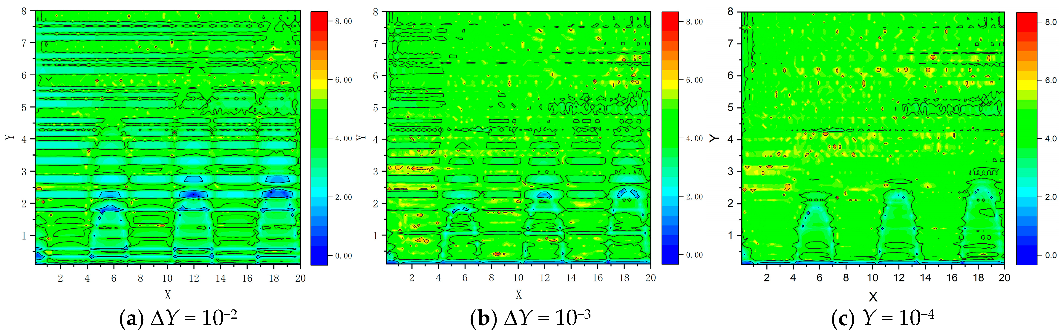
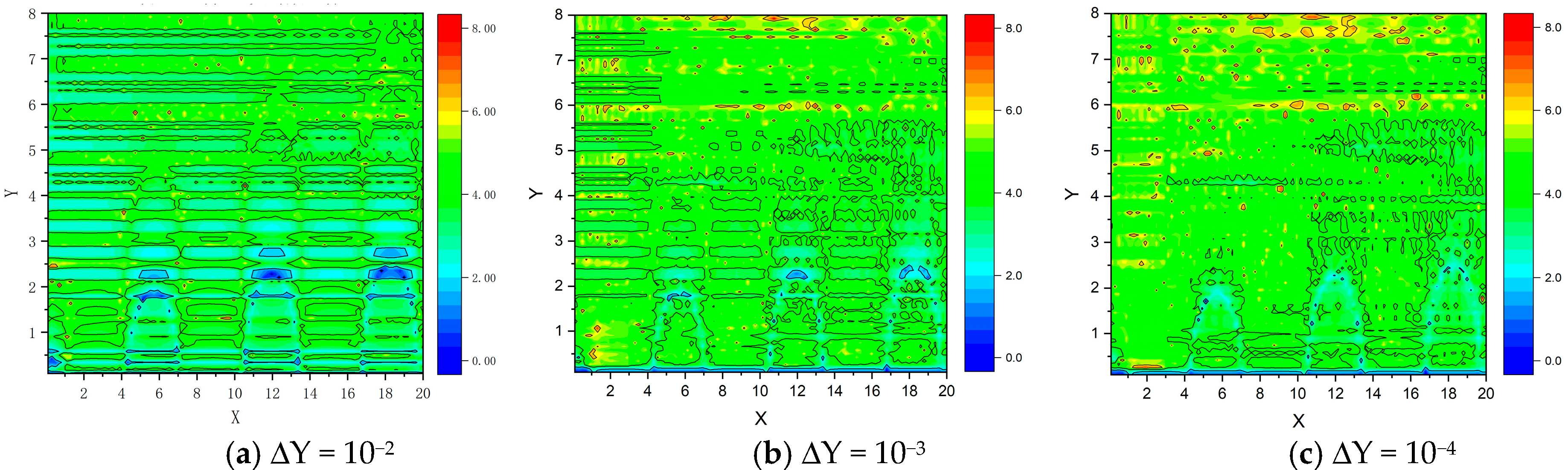
The influence of recursive step ΔY on errors and efficiency

Five sets of recursive step lengths ΔY = 10⁻², 5 × 10⁻³, 10⁻³, 5 × 10⁻⁴, 10⁻⁴ are selected for global forecasting. In this recursive process, the datum line spacing in the computational domain is uniformly set to 0.1. It can be observed that a smaller recursive step selected can yield better forecast results, but computational efficiency will decrease when choosing a smaller recursive step. Therefore, an appropriate recursive step should be selected during forecasting to improve forecast efficiency while maintaining sufficient forecast accuracy. The forecast error and computational time consumption (average time consumption refers to the ratio of the time taken to complete one forecast to the data scale, averaged over 10 forecasts) are shown in

Table 2. Error and computational time consumption with different recursive steps.

	Errors	Err < 10−2	10−2 < Err < 10−3	10−3 < Err < 10−4	10−4 < Err < 10−5	Err > 10−5	Average Time Consumption/μs
Step Size ΔY
10−2		3.49%	15.00%	34.86%	37.41%	9.24%	0.239
5 × 10−3		2.45%	15.09%	41.74%	32.31%	8.40%	0.259
10−3		1.40%	3.04%	26.31%	52.41%	16.84%	0.381
5 × 10−4		1.34%	3.14%	21.59%	55.21%	18.74%	0.547
10−4		1.13%	1.02%	14.69%	62.65%	20.51%	1.841

, and the corresponding partial error distribution cloud map is shown in Figure 5.

(2)

The influence of datum line interval on error and efficiency

This section investigates the influence of the spacing of the forecast datum line in-terval on the forecast results. In the computational domain, a datum line for recursion is arranged every 0.1/0.2/0.4 for Y₀. Based on these three different datum line arrangement schemes, the influence of the spacing of the datum line interval in the computational domain on errors is studied. In this set of forecasts, the recursive step is uniformly set to 10⁻³. It can be observed that if the datum line in the computational domain is arranged more densely, better forecast error results can be obtained, and the forecast efficiency can also be improved to some extent. The forecast errors and computational time consumption are shown in

Table 3. Errors and computational time consumption based on different baseline intervals.

	Forecast Error	Err < 10−2	10−2 < Err < 10−3	10−3 < Err < 10−4	10−4 < Err < 10−5	Err > 10−5	Average Time Consumption/μs
Baseline Interval
0.4		1.51%	4.07%	29.40%	49.94%	15.09%	0.889
0.2		1.57%	3.77%	27.33%	51.12%	16.21%	0.547
0.1		1.40%	3.04%	26.31%	52.41%	16.84%	0.381

, and the corresponding error distribution cloud map is shown in Figure 6.

4.2. Partitioned Training Recursive Prediction

Considering that within the range X ∈ [0, 20], the values of F(X, Y) or F_X(X, Y) on each datum line exhibit a certain degree of fluctuation, particularly near the free surface (when Y is small), which leads to relatively lower forecast accuracy near the free surface. The global forecast network presented earlier often requires a relatively high-complexity network to maintain high accuracy when training recursive datum lines. To optimize the forecasting program, the recursive datum line settings near the free surface are densified (the datum line interval near the free surface (X ≤ 1) region is adjusted to 0.05), and the recursive datum line network is trained with partitioning. The partitioning and network structure settings are shown in

Table 4. Datum line training area division and network setup.

Horizontal Coordinate X	Vertical Coordinate Y	Number of Network Nodes	Horizontal Coordinate X	Vertical Coordinate Y	Number of Network Nodes
[0.0, 3.0]	[0.1, 1.0]	48	[3.0, 20]	[3.1, 5.0]	16
	[1.1, 1.8]	8		[5.1, 6.0]	12
[3.0, 20]	[0.1, 1.0]	32		[6.1, 8.0]	8
	[1.1, 3.0]	24

.

After partitioning the datum lines for training and completing the refinement of datum line settings in the near-free-surface region, the prediction of F(X, Y) has been improved in both accuracy and efficiency. According to reference [18], the Green’s functions calculated by the recursive prediction method can meet the requirements of hydrodynamic calculations to a certain extent. The prediction errors and computational time consumption are shown in

Table 5. Errors and computational time consumption based on different recursion steps.

	Forecast Error	Err < 10−2	10−2 < Err < 10−3	10−3 < Err < 10−4	10−4 < Err < 10−5	Err > 10−5	Average Time Consumption/μs
Recursive Step Size ΔY
10−2		2.97%	14.35%	37.56%	33.18%	11.94%	0.166
5 × 10−3		2.38%	14.74%	43.20%	29.76%	9.91%	0.181
10−3		1.43%	2.69%	31.55%	43.32%	21.02%	0.298
5 × 10−4		1.37%	2.98%	26.69%	48.57%	20.28%	0.464
10−4		1.18%	1.58%	20.91%	50.52%	25.81%	1.675

, and the corresponding partial error distribution cloud maps are shown in Figure 7.

4.3. Forecast Efficiency Comparison

The pulsating source recursive prediction method is applied to compute Green’s functions for different data scales. The method used for testing in this paper is the partitioning method introduced in Section 4.2 (with the recursive step set to 10⁻³). The comparison methods included the Romberg integration method proposed by Newman [3], the global approximation method proposed by Wu et al. [11], and the global machine learning method proposed by Chang et al. [13].

The range of independent variables for the test input is X ∈ [0, 20], Y ∈ [0, 8]. The sampling interval is adjusted to obtain different test data. The computer used for testing had a CPU model of Inter(R) Core(TM) i5−8250U CPU @ 1.60 GHz. The results are shown in

Table 6. Comparison of forecasting efficiency for Green’s functions.

	Methods	Pulsating Source Recursive Prediction	Romberg Integration	Global Approximation (Wu)	Machine Learning (Chang)
Test Scale
400,000		0.281 $\mathsf{\mu }\mathrm{s}$	1.621 $\mathsf{\mu }\mathrm{s}$	0.562 $\mathsf{\mu }\mathrm{s}$	3.055 $\mathsf{\mu }\mathrm{s}$
800,000		0.316 $\mathsf{\mu }\mathrm{s}$	1.617 $\mathsf{\mu }\mathrm{s}$	0.589 $\mathsf{\mu }\mathrm{s}$	3.164 $\mathsf{\mu }\mathrm{s}$
1,600,000		0.307 $\mathsf{\mu }\mathrm{s}$	1.619 $\mathsf{\mu }\mathrm{s}$	0.587 $\mathsf{\mu }\mathrm{s}$	2.961 $\mathsf{\mu }\mathrm{s}$

.

It can be observed that, with the selection of an appropriate recursive step, the pulsating source recursive prediction method proposed in this paper far surpasses the Romberg numerical integration method and Chang‘s machine learning method in prediction efficiency, slightly outperforms Wu’s global approximation method, and achieves remarkable prediction efficiency within the set prediction range, demonstrating certain advantages in terms of computing efficiency.

5. Verification of Green’s Function Applications

In this chapter, the free-surface Green’s function will be calculated using the pulsating source recursive prediction method proposed in this paper, and then the hydrodynamic forces of different ships will be solved to verify the practical effectiveness of the method. The hydrodynamic calculations involve the following: ship motion response, wave diffraction forces, and hydrodynamic coefficients (added mass and damping coefficients). The calculation formulas for the hydrodynamic coefficients can be found in Section 2.1, while the calculations for wave diffraction forces and motion response can be referred to in References [1,2].

5.1. Numerical Examples

To validate the prediction program, this study adopted the container ship S175 and a bulk carrier as test objects. The hydrodynamic results from the proposed method are compared with those obtained using the three-dimensional pulsating source speed correction method (Romberg integration method). Main parameters and particulars of the S175 container ship and the bulk carrier are listed in

Table 7. Main parameters and particulars of container ship and bulk carrier.

Parameters	Symbols	S175	Bulk Carrier
Length between perpendiculars	LPP	175 m	295.2 m
Breadth	B	25.4 m	50.0 m
Draft	T	9.5 m	18.5 m
Waterplane area	AW	3156 m2	13,798.8 m2
Ship displacement	∇	24742 t	233,928 t
Height of gravity center	zg	9.52 m	14.28 m
Longitudinal position of gravity center	xg	−2.48 m	0.0 m
Longitudinal radius of gyration	Kyy	0.24 Lpp	0.25 Lpp
Natural rolling period	Tϕ	18 s	5.88 s
Molded depth	H	15.4 m	25.0 m

.

In the water of infinite depth and the incident wave of direction angle of 180°, the ship motion response, wave diffraction forces, and hydrodynamic coefficients of ship S175 are calculated. For the bulk carrier, its motion responses are calculated at a speed of 12 kn, with wave angles ranging from 0 to 180 degrees (at 45-degree intervals), and compared with experimental data. The experiment was conducted at the Deepwater Offshore Basin of Shanghai Jiao Tong University. The scale ratio of the ship model is 1:60. The basic dimensions of the basin are length 50.0 m, width 40.0 m, and depth 10.0 m. Among them, the ship motion data was measured by the QUALISYS motion testing system. The computational mesh numbers of S175 and bulk carrier are 800 and 1360, respectively, as shown in Figure 8.

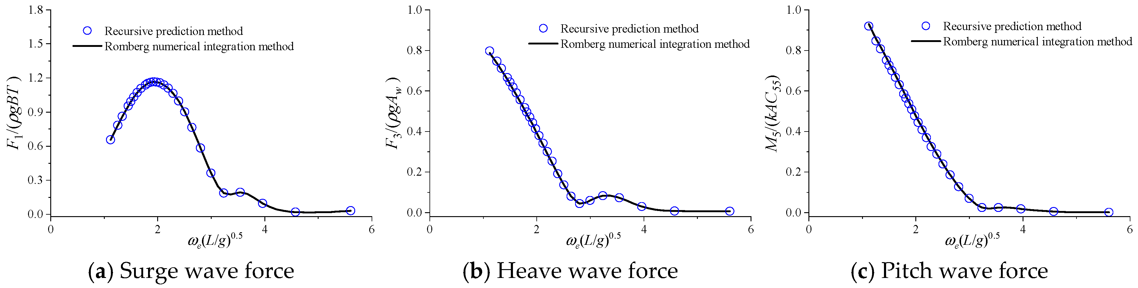
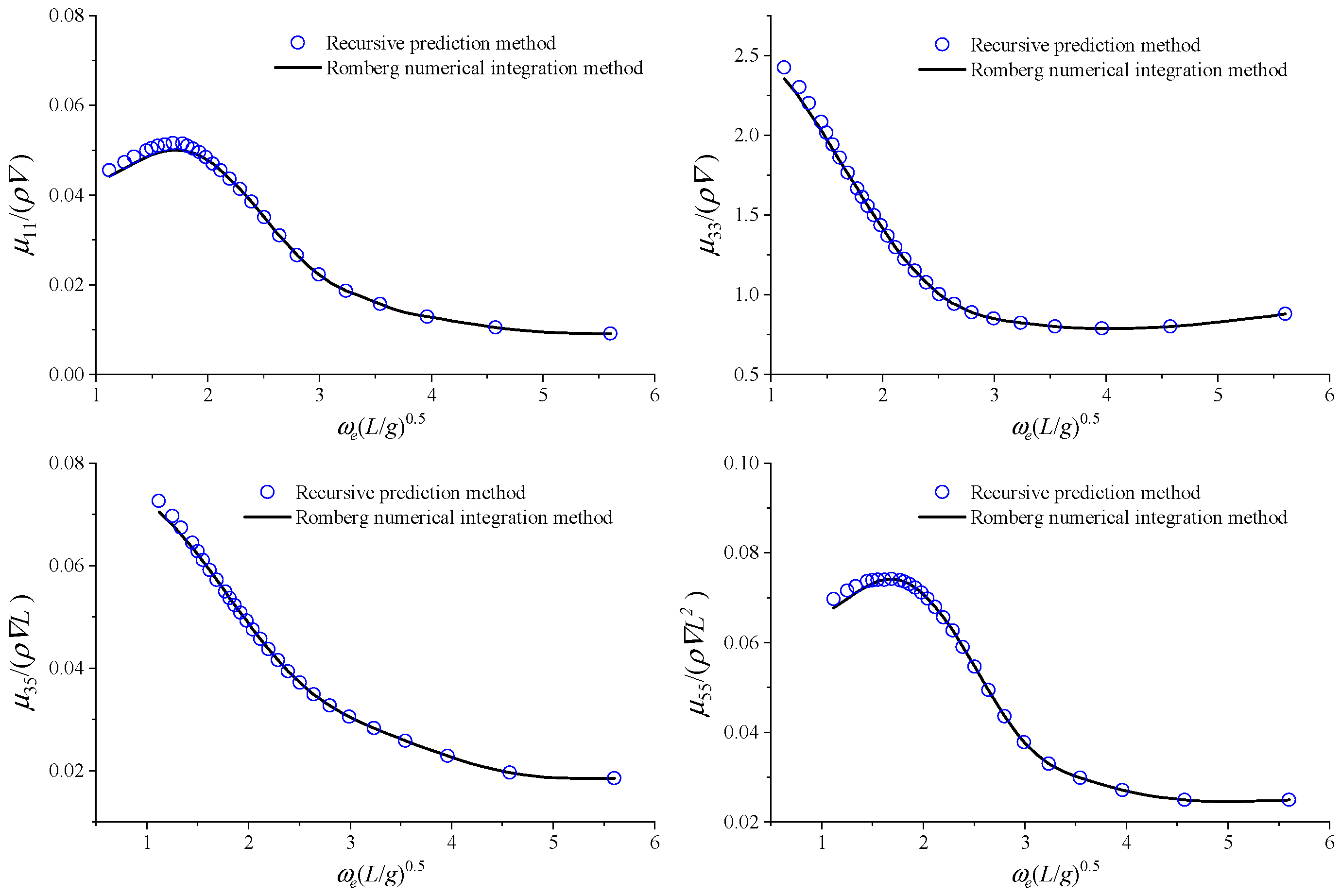
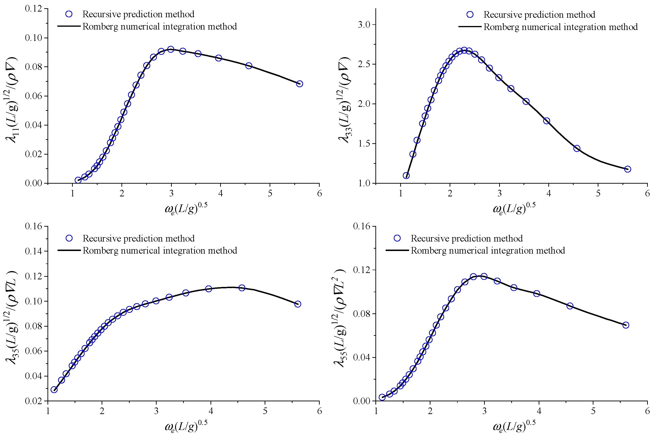
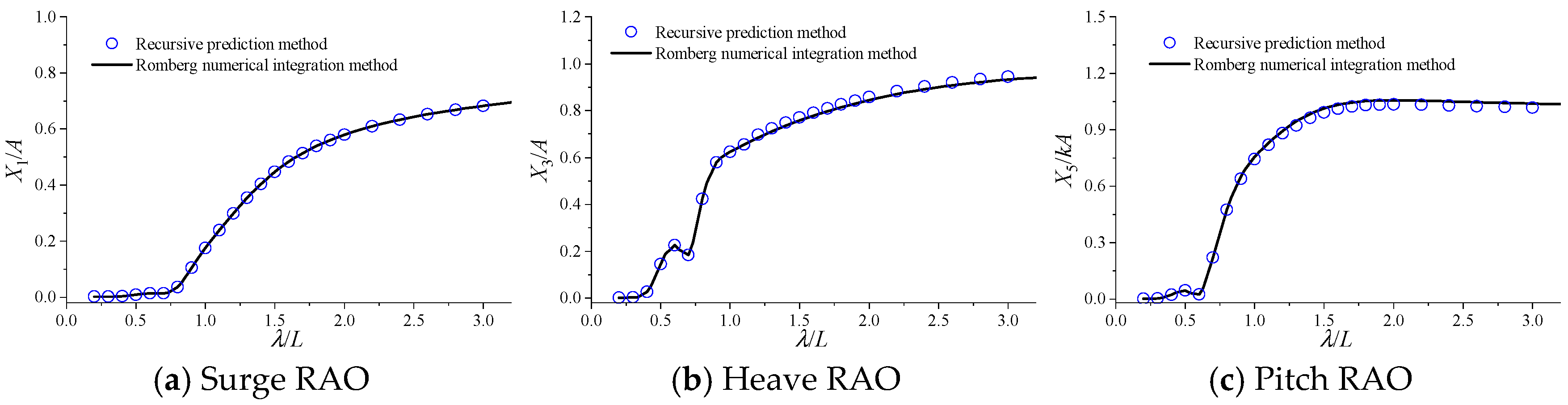
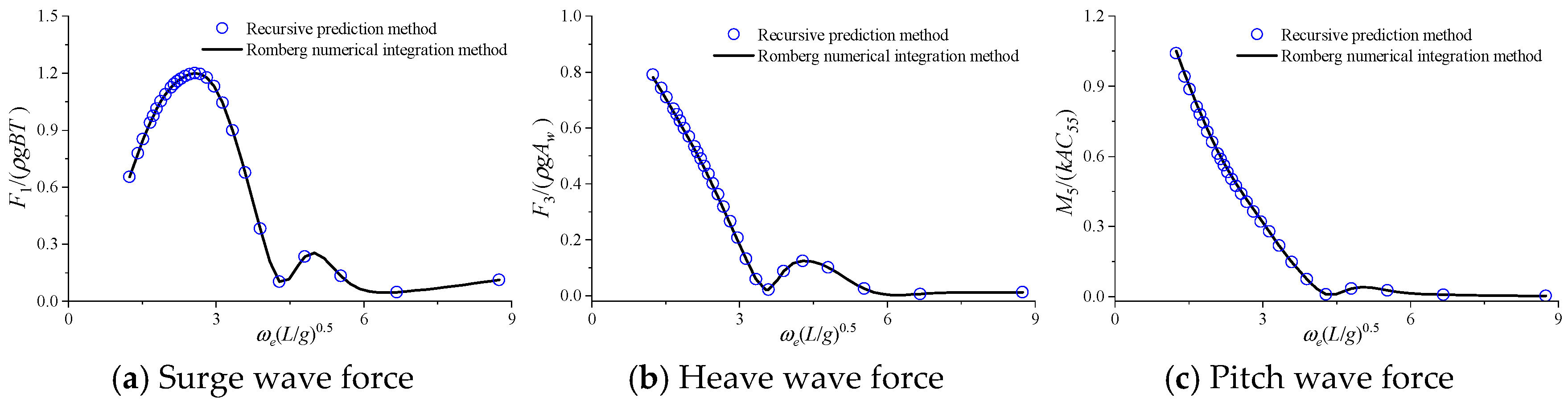
5.2. Case of Ship Motion in Waves Without Speed

The hydrodynamic calculation results of S175 oscillating without speed in head waves in the water of infinite water depth were non-dimensionalized, and they are shown as follows.

In Figure 9, the calculation results of motion response are plotted, and the horizontal coordinate represents the ratio of wavelength λ to ship length L.

In the figure, the blue circles represent RAO results calculated by the pulsating source recursive prediction method, while the black line represents those calculated by the 3DP method with the Romberg integration method. As shown in Figure 9, there are minor errors in the prediction of the heave and pitch motion of S175 in long waves. However, the overall prediction trend remains consistent, and the forecast results of motion responses of each motion mode are accurate and reasonable.

The calculated amplitudes of the first-order wave forces, including surge force, heave force, and pitch force, are shown in Figure 10. The horizontal coordinate represents dimensionless frequency ω_e(L/g)^0.5 (ω_e is the encounter frequency).

As shown in Figure 10, the predicted amplitudes of surge, heave, and pitch wave forces calculated by the two methods are basically consistent.

The calculation results of some hydrodynamic coefficients are also shown in Figure 11 and Figure 12. As shown in the figures, the predicted results of added mass and damping coefficients exhibit minor errors at certain frequencies, while the overall prediction trend remains consistent.

5.3. Case of Ship Motion in Waves with Forward Speed

The hydrodynamic calculation results for container ship S175 advancing in head waves (F_n = 0.10) in the water of infinite depth are as follows.

The calculation results of the motion response are shown in Figure 13. As shown in Figure 13, the calculated results of the two methods for surge motion are basically consistent. For heave and pitch motion response, the two methods show very small deviations in the long waves, but the overall prediction trend is consistent, and the prediction results for other motion modes are accurate and reasonable.

The calculated amplitudes of first-order wave forces are shown in Figure 14. It can be seen that the predictions for the amplitudes of surge, heave, and pitch wave forces by the two methods are basically consistent.

The calculation results of some hydrodynamic coefficients are shown in Figure 15 and Figure 16. It can be seen that the predicted results of added mass exhibit minor errors at certain frequencies, while the overall prediction trend remains consistent. For the damping coefficient, very slight deviations occur at some frequencies, but the predicted results are overall consistent.

The calculated results of motion responses for the bulk carrier at a speed of 12 kn under different wave directions are shown in Figure 17, Figure 18, Figure 19 and Figure 20, where “EXP” represents the experimental value. It can be seen that the calculation results of the two methods are basically consistent, and they agree well with the experimental values, indicating that the method with enough accuracy.

6. Conclusions

This paper analyzes the mathematical relationship between the Green’s function and its partial derivatives, then proposes a recursive prediction method based on machine learning theory for calculating the frequency-domain infinite water depth zero-speed free-surface Green’s function. This method is also applied to compute the motion response, wave forces, and hydrodynamic coefficients of the S175 container ship and a bulk carrier, verifying the method’s effectiveness. It can be concluded as follows:

(1)

With an appropriate recursive step size in the vertical direction, the predicted result of F(X, Y) can achieve an accuracy of 10⁻³ to 10⁻⁶, with most prediction points reaching at least 10⁻⁴ accuracy, which generally meets the requirements of ship hydrodynamic calculations.

(2)

If an appropriate recursive step size is selected, the pulsating source recursive prediction method for calculating the Green’s function far surpasses numerical methods in computational efficiency within the defined computational domain, and it is comparable to the analytical method.

(3)

Theoretically, if the spacing of the baseline arrangement in the computational domain can be reduced, better prediction accuracy and efficiency can be achieved. More refined partition training can further reduce the complexity of the neural networks used, thereby improving prediction efficiency. The proposed method maintains a certain advantage in efficiency while ensuring accuracy.

(4)

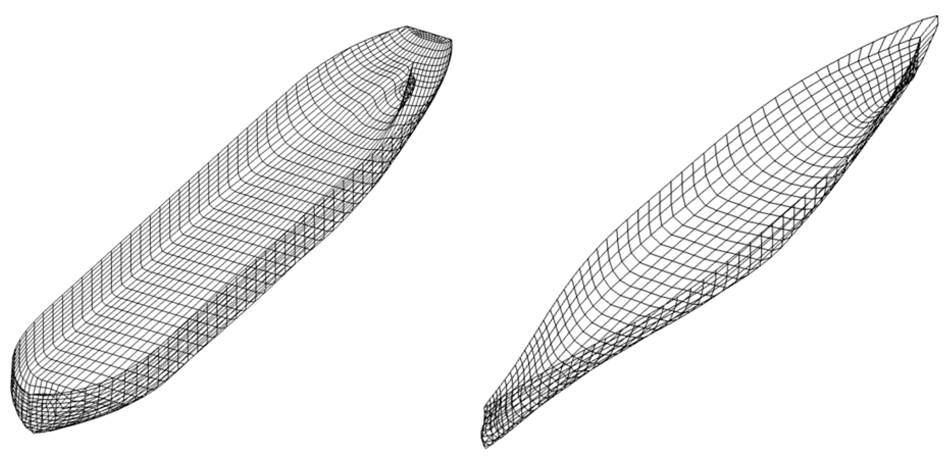
The free-surface Green’s function and its partial derivatives are calculated using the pulsating source recursive prediction method and applied to the hydrodynamic calculations of the S175 container ship and a bulk carrier. The results are generally accurate, indicating that the method meets the needs of ship hydrodynamic calculations. The proposed method is universal and can also be applied to hydrodynamic calculations for other types of ships.

(5)

Since the values of the free-surface Green’s function or its partial derivatives in the far field are extremely small and vary gently, the pulsating source recursive prediction method does not yield satisfactory results. Thus, the method has certain limitations. For hydrodynamic calculations of large floating bodies like floating platforms, the pulsating source recursive prediction method can be used in the near field, while analytical methods are recommended for the far field.

References

1. Zhu, R.C.; Miao, G.P. Theory of Ship Motion in Waves; Shanghai Jiao Tong University Press: Shanghai, China, 2019. [Google Scholar]
2. Newman, J.N. Marine Hydrodynamics; MIT Press: Cambridge, MA, USA, 1977. [Google Scholar]
3. Noblesse, F. The Green function in the theory of radiation and diffraction of regular water waves by a body. J. Eng. Math. 1982, 16, 137–169. [Google Scholar] [CrossRef]
4. Newman, J.N. Double-precision evaluation of the oscillatory source potential. J. Ship Res. 1984, 28, 151–154. [Google Scholar] [CrossRef]
5. Newman, J.N. Algorithms for the free-surface Green function. J. Eng. Math. 1985, 19, 57–67. [Google Scholar] [CrossRef]
6. Newman, J.N. The approximation of free-surface Green functions. In Wave Asymptotics; Martin, P.A., Wickham, G.R., Eds.; Retirement Meeting for Professor Fritz Ursell, University of Manchester; Cambridge University Press: Cambridge, UK, 1992. [Google Scholar]
7. Wang, R.C. The numerical approach of three dimensional free-surface green function and its derivates (Frequency domain-infinite depth). J. Hydrodyn. (A) 1992, 3, 277–286. [Google Scholar]
8. Zhou, Q.B.; Zhang, G.; Zhu, L.S. The fast calculation of free-surface wave green function and its derivatives. Chin. J. Comput. Phys. 1999, 2, 3–10. [Google Scholar]
9. Duan, W.Y.; Yu, D.H.; Shen, Y. Algorithm for infinite depth water wave green function and its high order derivatives. J. Ship Mech. 2016, 20, 10–22. [Google Scholar]
10. Yao, X.L.; Sun, S.L.; Zhang, A.M. Efficient Calculation of 3D Frequency-domain Green Functions. Chin. J. Comput. Phys. 2009, 26, 564–568. [Google Scholar]
11. Wu, H.; Zhang, C.; Zhu, Y.; Li, W.; Wan, D.; Noblesse, F. A global approximation to the Green function for diffraction radiation of water waves. Sci. Direct Eur. J. Mech. B/Fluids 2017, 65, 54–64. [Google Scholar] [CrossRef]
12. Shan, P.H.; Zhu, R.C.; Wang, F.H.; Wu, J. Efficient approximation of free-surface Green function and OpenMP parallelization in frequency-domain wave—Body interactions. J. Mar. Sci. Technol. 2019, 24, 479–489. [Google Scholar] [CrossRef]
13. Chang, H.Y.; Zhu, R.C.; Huang, S. Preliminary study on prediction of pulsating source Green function based on machine learning. Ocean. Eng. 2020, 38, 131–141. [Google Scholar]
14. Hess, D.E.; Roddy, R.F.; Faller, W.E. Uncertainty Analysis Applied to Feedforward Neural Networks. Ship Technol. Res. 2007, 54, 114–124. [Google Scholar] [CrossRef]
15. Zhou, Z.H. Machine Learning; Tsinghua University Press: Beijing, China, 2016. [Google Scholar]
16. Fischer, A.; Izmailov, A.F.; Solodov, M.V. The Levenberg–Marquardt method: An overview of modern convergence theories and more. Comput. Optim. Appl. 2024, 89, 33–67. [Google Scholar] [CrossRef]
17. Amini, K.; Rostami, F.; Caristi, G. An efficient Levenberg-Marquardt method with a new LM parameter for systems of nonlinear equations. Optimization 2018, 67, 637–650. [Google Scholar] [CrossRef]
18. Liang, H.; Wu, H.; Noblesse, F. Validation of a global approximation for wave diffraction-radiation in deep water. Appl. Ocean. Res. 2018, 74, 80–86. [Google Scholar] [CrossRef]
Figure 1. Structure diagram of neural network.
Jmse 13 01488 g001
Figure 2. Numerical distribution of Green’s function in the computational domain.
Jmse 13 01488 g002
Figure 3. Benchmark function plotting on the datum lines.
Jmse 13 01488 g003
Figure 4. Schematic diagram of neural network structure.
Jmse 13 01488 g004
Figure 5. Error distribution of forecast results with different recursive steps.
Jmse 13 01488 g005
Figure 6. Error distribution of forecast results based on different datum line intervals.
Jmse 13 01488 g006
Figure 7. Error distribution of forecast results based on different recursion steps (partitioned).
Jmse 13 01488 g007
Figure 8. Computational mesh for S175 and bulk carrier.
Jmse 13 01488 g008
Figure 9. RAO calculation results for S175 without speed.
Jmse 13 01488 g009
Figure 10. Calculation results of diffraction force amplitude for S175 without speed.
Jmse 13 01488 g010
Figure 11. Calculation results of added mass for S175 without speed.
Jmse 13 01488 g011
Figure 12. Calculation results of damping coefficient for S175 without speed.
Jmse 13 01488 g012
Figure 13. RAO calculation results for S175 with speed.
Jmse 13 01488 g013
Figure 14. Calculation results of diffraction force for S175 with speed.
Jmse 13 01488 g014
Figure 15. Calculation results of added mass for S175 with speed.
Jmse 13 01488 g015
Figure 16. Calculation results of damping coefficient for S175 with speed.
Jmse 13 01488 g016
Figure 17. Calculation results of motion response for the bulk carrier at a speed of 12 kn in head waves.
Jmse 13 01488 g017
Figure 18. Calculation results of motion response for the bulk carrier at a speed of 12 kn in bow oblique and beam waves.
Jmse 13 01488 g018
Figure 19. Calculation results of motion response for the bulk carrier at a speed of 12 kn in quartering sea.
Jmse 13 01488 g019
Figure 20. Calculation results of motion response for the bulk carrier at a speed of 12 kn in following waves.
Jmse 13 01488 g020