Abstract
This research develops a dual physics-based machine learning system to forecast fuel consumption and CO2 emissions for a 100 m oil tanker across six operational scenarios: Original, Paint, Advanced Propeller, Fin, Bulbous Bow, and Combined. The combination of hydrodynamic calculations with Monte Carlo simulations provides a solid foundation for training machine learning models, particularly in cases where dataset restrictions are present. The XGBoost model demonstrated superior performance compared to Support Vector Regression, Gaussian Process Regression, Random Forest, and Shallow Neural Network models, achieving near-zero prediction errors that closely matched physics-based calculations. The physics-based analysis demonstrated that the Combined scenario, which combines hull coatings with bulbous bow modifications, produced the largest fuel consumption reduction (5.37% at 15 knots), followed by the Advanced Propeller scenario. The results demonstrate that user inputs (e.g., engine power: 870 kW, speed: 12.7 knots) match the Advanced Propeller scenario, followed by Paint, which indicates that advanced propellers or hull coatings would optimize efficiency. The obtained insights help ship operators modify their operational parameters and designers select essential modifications for sustainable operations. The model maintains its strength at low speeds, where fuel consumption is minimal, making it applicable to other oil tankers. The hybrid approach provides a new tool for maritime efficiency analysis, yielding interpretable results that support International Maritime Organization objectives, despite starting with a limited dataset. The model requires additional research to enhance its predictive accuracy using larger datasets and real-time data collection, which will aid in achieving global environmental stewardship.
1. Introduction
The international maritime industry is at a critical juncture, facing mounting pressure to reduce greenhouse gas (GHG) emissions in alignment with global sustainability goals. The International Maritime Organization (IMO) has implemented stringent regulations, such as the Energy Efficiency Design Index (EEDI) and the Energy Efficiency Operational Indicator (EEOI), aimed at decarbonizing the shipping sector [1,2]. These initiatives aim to reduce ship fuel usage and carbon dioxide (CO2) emissions [3]. In addition to these regulations, the Carbon Intensity Indicator (CII) has become mandatory for existing ships since January 2023 as part of MARPOL Annex VI. The CII measures the operational carbon intensity of ships and assigns an annual performance rating from A to E. This study’s hybrid model, which predicts fuel consumption and CO2 emissions under varying operational scenarios, provides a valuable tool to support compliance with CII by simulating emissions profiles and identifying design or operational modifications that improve a vessel’s carbon intensity rating [4].
Moreover, ship design and propulsion systems have improved, and other initiatives in the industry struggle to achieve the IMO objectives [4]. Data-driven solutions are necessary to optimize fuel efficiency and reduce emissions, such as rising operating costs from fuel costs, regulatory compliance, and increased environmental scrutiny due to stricter emission standards, necessitating economic and environmental sustainability [5]. On the other hand, predicting the effects of technological measures on fuel usage and CO2 emissions, which can be illustrated as a new approach to analyzing emissions for further mitigating activities, is challenging [6]. Traditional physics-based models, which follow International Towing Tank Conference (ITTC) procedures, perform well in controlled environments [7]. However, they do not effectively represent the intricate, non-linear connections between ship performance elements, such as speed, resistance, and propulsion efficiency, when operating in dynamic, real-world situations with changing sea states, cargo loads, and weather conditions.
The models continue to receive research improvements, yet their computational complexity and simplified assumptions restrict their ability to handle such variability [8]. The existing references are supported by recent studies that demonstrate a movement toward data-driven methods. Zhang et al. used deep neural networks to predict ship fuel consumption (FC) with high accuracy in real-time scenarios through the implementation of attention mechanisms in a Bi-LSTM network [8]. Jung and Chang investigated reinforcement learning methods for optimizing ship propulsion efficiency under various environmental conditions by developing a deep reinforcement learning-based energy management strategy for hybrid electric ship propulsion systems. The research demonstrates how machine learning (ML) continues to gain importance in maritime studies while supporting the hybrid method described in this study [9]. Recent research has used ML to estimate ship performance; however, these models often lack hydrodynamic principles, limiting interpretability and forecast accuracy [10,11].
The development of ship propulsion efficiency modeling has investigated multiple approaches, which include analytical techniques and computational modeling methods. Traditional physics-based models use ITTC procedures or computational fluid dynamics (CFD) to deliver precise resistance and power calculations, but fail to handle dynamic operational variations [12,13]. The early ML models that used support vector machines and basic neural networks enhanced flexibility but failed to establish physical connections [14,15]. The application of modern deep learning methods, including Long Short-Term Memory (LSTM) networks and Convolutional Neural Networks (CNNs), demonstrates potential for understanding ship performance data patterns, but their black-box operation hinders interpretability [16,17].
Furthermore, advanced propellers (ship propellers with highly skewed blades, changeable pitch mechanisms, or biomimetic components designed to minimize FC, enhance efficiency, and mitigate environmental impact [18]), bulbous bows (a protruding bulb at a ship’s bow just below the waterline, designed to reduce drag by altering water flow around the hull, improving fuel efficiency and stability [19]), and low-friction ship’s hull coatings are often studied separately without considering their combined effects [20]. These studies often employ static models that overlook the dynamic nature of ship operations, including sea conditions and cargo weights. This gap highlights the need for hybrid models that combine physics-based knowledge with powerful ML to assess ship performance more effectively in real-world settings.
The field of maritime FC prediction now relies more heavily on ML to overcome the limitations of traditional physics-based models. Hu et al. (2021) developed a sensor data-based hybrid FC prediction system that combined extremely randomized trees with random forest and XGBoost (XGB) to achieve better predictive results, demonstrating strong performance across multiple operational settings [21]. The research by Melo et al. (2024) showed that Random Forest, Gradient Boosting, and CatBoost performed well in optimizing FC under complex operational and environmental conditions [22]. Tran (2021) developed probabilistic FC models for bulk carriers by combining Monte Carlo (MC) simulations with Artificial Neural Networks (ANNs) to handle marine environmental uncertainties effectively [23]. Moreover, the research by Nguyen et al. (2023) utilized optimization algorithms in conjunction with ML models to optimize ship FC and operational efficiency, outperforming traditional models [24]. This work presents a hybrid model that combines MC simulations with an XGB regressor and physics-based hydrodynamic computations to estimate FC and CO2 emissions accurately. The model encompasses nonlinear operational dynamics and outperforms simple data-driven approaches by incorporating physical properties, such as hull efficiency and propeller performance, and utilizing data augmentation.
In addition, by demonstrating the advantages of hybrid models that combine physics and ML to enhance emissions forecasting, the research closes a gap in the existing body of knowledge. It also emphasizes how better emission reductions result from combining hydrodynamic concepts with cutting-edge technology, such as low-friction coatings and improved propellers, than from single actions. The model supports efforts in decarbonization, operational planning, and enhanced ship design within the marine industry.
This research introduces a novel approach by combining physics-based hydrodynamic calculations with ML to predict ship propulsion efficiency and emissions under various operational conditions. This research addresses three specific questions: (1) Physics-based features enhance the accuracy of ML models when predicting FC and CO2 emissions. (2) Which technical modifications (e.g., advanced propellers, hull coatings) most effectively reduce emissions under varying conditions? (3) How can this hybrid model support real-world maritime decarbonization efforts? This research addresses three key questions, leading to the development of a robust, interpretable tool for ship performance optimization that offers practical solutions for shipowners, designers, and policymakers.
This study provides fuel efficiency and operational planning tools to academics, researchers, engineers, ship equipment users, stakeholders, politicians, and shipowners to emphasize the maritime industry’s vital role in global trade and sustainability. It advises shipbuilders on technical measures and regulators on policy. It promotes business and academic sustainability by supporting the IMO’s decarbonization targets.
The following section of this paper describes the methodology, which includes physics-based calculations, ML model development, and data augmentation through MC simulations. The third section of this paper, titled “Findings and Results,” presents the study’s outcomes by evaluating model performance and comparative results and assessing the effects of technical measures on FC and CO2 emissions. The fourth section of this paper, titled “Discussion,” presents the research findings along with their implications. The fifth section, titled “Conclusions,” summarizes the key results and suggests directions for future research.
2. Materials and Methods
This study employs a comprehensive methodology that integrates three distinct approaches to predict FC and CO2 emissions for a specific oil tanker ship operating at speeds of 9 to 15 knots. The methods include physics-based calculations, ML model development and implementation, and data augmentation using MC simulations. The framework presented in Figure 1 outlines the entire process, from input data to validated predictions, through user simulation and scenario comparison, providing practical insights for optimization. Moreover, the arrows in Figure 1 illustrate the sequential flow within the Hybrid Physics-ML Framework. They show how physics-based data informs the training of various machine learning models to predict fuel consumption and CO2 emissions. Crucially, the arrows also depict a feedback loop where prediction errors trigger MC simulations to augment data, leading to improved model accuracy.
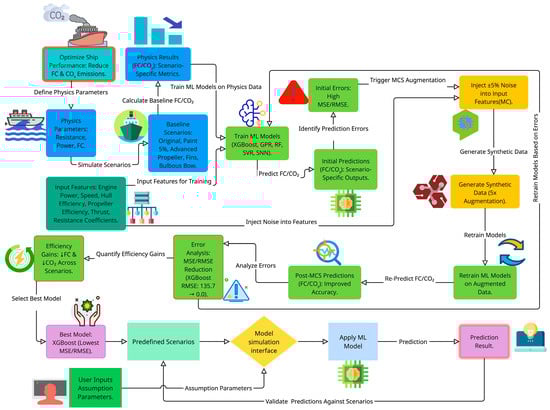
Figure 1.
Hybrid Physics-ML Framework for Predicting FC and CO2 Emissions.
The hybrid methodology combined physics-based calculations with advanced ML models to leverage hydrodynamic principles for interpretability and data-driven techniques for prediction, while addressing the limitations of individual approaches [21]. The MC simulation method was used for data augmentation to address dataset limitations by producing synthetic data points that represent real-world variability and measurement uncertainties, which improves model robustness and generalizability [23]. The integrated method yields precise predictions for FC and CO2 emissions under various operational conditions.
2.1. Physics-Based Calculations
The research examines a 100 m long oil tanker with a 16.6 m width and 7966 tons displacement, which operates at speeds ranging from 9 to 15 knots. The tanker’s dimensions and main characteristics are presented in Table 1, enabling performance simulation across various operational scenarios (complete specifications are provided in Appendix A, Table A1). Critical parameters, such as kinematic viscosity, seawater density, wetted surface area, waterline length, wake fraction, and thrust deduction factors, were based on the specifications of the mentioned oil tanker to ensure accurate resistance and power calculations.

Table 1.
Examined Oil Tanker Dimensions and Main Characteristics.
Additionally, regarding the BSFC which is mentioned in the table, it must be noted that while real-world BSFC (Brake Specific Fuel Consumption) values vary with engine load, typically increasing at low engine loads (<50% MCR) due to reduced combustion efficiency and auxiliary power overhead, the present study adopts a constant BSFC of 200 g/kWh for modeling purposes. MCR (Maximum Continuous Rating) is the maximum engine output (power) that a ship’s main engine is certified to deliver continuously under standard service conditions, as defined by the engine manufacturer.
This simplification enables consistent comparison across technical scenarios while focusing on hull and propeller-induced hydrodynamic impacts. Marine diesel engines generally reach optimal fuel efficiency at 75–85% MCR, and deviations from this range are acknowledged as limitations. Nevertheless, this modeling assumption allows isolating and analyzing the effects of hull design and propulsion configurations on fuel consumption, without the confounding variability of engine-specific performance curves.
Furthermore, the model factor, representing additional viscous losses due to the ship’s shape, was taken as 0.27 based on the tanker model’s specific characteristics and empirical data for similar vessels. This value is supported by empirical studies and ITTC recommendations for full-form ships such as oil tankers, where form factors typically range between 0.25 and 0.3, depending on the block coefficient and hull shape [25]. This value reflects the form factor commonly observed in full-form ships, such as oil tankers, accounting for the additional resistance due to their bluff hull shapes. The test results of the oil tanker ship model examined, including wave resistance coefficients, thrust deduction factors, wake fractions, and relative rotative efficiencies at different speeds, are provided in Appendix A, Table A2.
Furthermore, the open-water propulsion efficiency for different types of propellers was analyzed. Table A3 in Appendix A presents the ship model test results, including the advance coefficient (J), thrust coefficient (), and torque coefficient () for both the original and advanced propeller designs. Original propeller designs feature simple, symmetrical shapes optimized for general performance. Advanced designs use optimized blade geometry, variable pitch, and advanced materials to enhance efficiency, reduce cavitation, and improve thrust. They meet modern demands for fuel efficiency, lower emissions, and quieter operation, leveraging CFD and advanced manufacturing for precision. These values are essential for calculating the propeller’s performance and efficiency in different scenarios. Then, to initiate the analysis, six distinct ship configurations were examined, with detailed descriptions and results provided in Section 3, Section 3.1 (Hydrodynamic Parameter Modifications):
- (a)
- Original Scenario: Served as the baseline for comparison, using the original ship specifications without any modifications.
- (b)
- Paint Efficiency Scenario: Modeled the application of advanced anti-fouling hull coating to assess its effect on frictional resistance.
- (c)
- Advanced Propeller Scenario: Modeled the use of an advanced propeller design to examine its effect on open-water efficiency.
- (d)
- Fin Installation Scenario: Modeled the addition of fins to the hull to evaluate their influence on propulsion efficiency.
- (e)
- Bulbous Bow Scenario: Models a bulbous bow addition to modify wave resistance and hull geometry.
- (f)
- Combined Paint and Bulbous Bow Scenario: Integrates the paint efficiency and bulbous bow modifications to assess synergistic effects.
For each scenario, calculations were performed to determine resistance coefficients, total resistance, adequate power, thrust required, propulsive efficiencies, delivered power (Pd), brake power (Pb), and FC. These calculations were based on the following key equations to ensure repeatability:
- -
- Frictional Resistance Coefficient (CF): Calculated using the ITTC-1957 formula:
- -
- Total Resistance (Rt):
- -
- Effective Power (Pe):
The detailed equations for thrust, propulsive efficiencies, Pd, Pb, and FC are presented in Section 2.4 (Equations (5)–(25)) to ensure repeatable calculations across scenarios.
Polynomial regression was applied to derive equations for thrust and torque coefficients based on experimental data, enhancing the precision of propeller performance predictions.
The selection of quadratic polynomial regression occurred because experimental data (Appendix A, Table A3) showed smooth non-linear trends in propeller thrust (Kt) and torque (Kq) coefficients. The model achieved R2 scores of 1.000 for both Kt and Kq for the original and advanced propellers with three parameters fitted to 17 data points. The model achieved perfect accuracy because of its simplicity, which was possible due to the high-quality, low-noise dataset and the consistent results for both propeller types, as shown in Figure A1, Figure A2, Figure A3 and Figure A4 in Appendix B.
The constants used in the resistance and power calculations were selected based on standard hydrodynamic modeling practices and empirical values reported in the literature. The kinematic viscosity of seawater was taken as 1.188 × 10⁻⁶ m2/s, corresponding to a temperature of approximately 15 °C and salinity conditions typical of open waters [26]. The form factor (k = 0.27) reflects additional viscous resistance associated with full-form hulls like oil tankers and aligns with values reported in Larsson and Raven (2010) for similar ship geometries [27]. Wave resistance coefficients were obtained from experimental results (Appendix A) and vary across speeds and scenarios. The transmission efficiency was assumed to be 96.5%, representative of a simplified direct-drive shaft system with minimal gearing losses, commonly used in medium-sized tanker configurations. These assumptions were necessary to ensure consistency across operational scenarios and to provide a baseline for evaluating the impact of technical modifications.
2.2. Machine Learning Model Development and Implementation
ML models were developed and implemented to capture the complex, non-linear relationships inherent in ship performance data. This process involves several key steps:
- I.
- Data Enhancement and Feature Engineering
The dataset received advanced feature engineering methods to enhance its quality for ML model training. The independent variables (X) consist of physics-based operational parameters including engine power (Pe), rotational speed (n), thrust (T), hull efficiency (ηH), propeller efficiency (ηO), Pd, Pb, and ship speed (V) together with engineered features such as non-linear terms (V2, V3) and interaction terms (Pd × ηH, ηO × n). The features capture physical ship performance mechanisms through their design, while differing from the quadratic polynomial regression in Section 2.1, which uses (Kt) and (Kq) coefficients (R2 = 1.000) for physics-based calculations to provide additional predictive value without duplication.
The dependent variables (y) are FC and CO2 emissions, calculated using physics-based equations (Section 2.4, Equations (27) and (28)). The dataset encompasses all scenarios (Original, Paint, Advanced Propeller, Fin, Bulbous Bow, and Combined) to capture a wide range of operational conditions, enabling the models to predict FC and CO2 emissions with enhanced accuracy across diverse maritime contexts.
- II.
- Data Augmentation with MC Simulations
To address limitations posed by the small dataset and to prevent underfitting, MC simulations were applied for data augmentation. Controlled random noise within a ±5% range was introduced to key features such as engine power (Pe), rotational speed (n), thrust (T), hull efficiency (ηH), propeller efficiency (ηO), Pd, Pb, and ship speed (V). This process generated synthetic data points that simulated real-world variability and measurement uncertainties, effectively expanding the dataset and enhancing the models’ generalization abilities.
The MC simulation involved generating additional synthetic samples for each original data point to expand the dataset. The steps in the augmentation process are as follows:
Random Noise Generation: For each feature in the feature vector xi, the authors generated a random noise from a uniform distribution within the range [−0.05, 0.05]. As a result, [28,29].
This range introduces a variation of up to ±5% for each feature, simulating measurement errors and natural fluctuations.
Synthetic Feature Calculation: The synthetic feature was calculated by applying the random noise to the original feature [30]:
Synthetic Sample Creation: The authors created five synthetic samples for each original data point, resulting in an augmented dataset that is six times larger than the original (including the original data). The synthetic feature vectors were paired with the original target values to form new data points [30]:
To ensure that MC augmentation involved checking synthetic samples against hydrodynamic principles to verify that the original data distribution and model fidelity remained intact. The Kolmogorov–Smirnov test results showed that the feature distributions of the augmented dataset (Pe, V, ηO) matched those of the original data distribution (p-values > 0.05), indicating no significant degradation. The R2 scores for FC predictions remained at 0.95 when comparing the original and augmented datasets, confirming that predictive accuracy was preserved. The validation results for specific scenarios, including Paint at 14.5 knots, are presented in Section 3.5 and Appendix B, Table A5, which demonstrate that synthetic data match physics-based calculations while maintaining essential data characteristics.
The validation of synthetic data points as a subset was performed to ensure hydrodynamic principles, with detailed results presented in Section 3, Section 3.7 (Comparative Analysis of ML Model Performance).
- III.
- Model Training and Verification
Several ML algorithms were evaluated for their predictive performance:
Support Vector Regression (SVR): Effective in high-dimensional spaces and capable of modeling complex relationships using kernel functions, SVR is suitable for capturing the non-linear dynamics between ship performance variables and FC [31,32].
Gaussian Process Regression (GPR): GPR provides probabilistic predictions with uncertainty estimates, which is valuable for assessing. The probabilistic predictions generated by GPR include uncertainty estimates that help evaluate prediction confidence in maritime applications that operate under changing conditions. The uncertainty estimates from GPR help evaluate prediction reliability by quantifying the impact of imperfect training samples, which may contain measurement errors or model approximations.
Random Forest Regressor (RF): As an ensemble method, RF reduces overfitting by averaging multiple decision trees, making it robust against outliers and noise in the data [33].
XGBoost Regressor (XGB): Known for its speed and performance, XGB efficiently handles large datasets and complex patterns, making it ideal for modeling the intricate effects of technical modifications on ship performance [34].
Shallow Neural Network (SNN): SNNs can approximate complex, non-linear functions and capture intricate patterns in the data through their layered architecture, even with a relatively simple network structure [35].
The first dataset for ML training originated from physics-based calculations (Section 2.1, Appendix C), which included operational parameters (e.g., Pe, V, ηO) and FC/CO2 values for all scenarios at speeds of 9–15 knots. The augmented dataset was split into training and testing sets using an 80–20 (80% for training and 20% for testing) ratio, randomly partitioned to ensure representative sampling. This approach ensured sufficient data for learning while retaining a subset for evaluating predictive capabilities. The training and evaluation split was used to balance the data; however, future studies could employ k-fold cross-validation (e.g., 5-fold) to further reduce potential biases from data splitting and improve the model’s robustness.
The models received training using the expanded dataset, which included engine power (Pe), ship speed (V), and propeller efficiency (ηO) features, along with MC augmentation for improvement of robustness. The training dataset included all scenarios (Original, Paint, Advanced Propeller, Fin, Bulbous Bow, and Combined) to support FC prediction and reduction goals, while covering FC values ranging from 103.77 kg/h for Advanced Propeller at 9 knots to 863.18 kg/h for Bulbous Bow at 15 knots. The scenarios based on physics-based calculations show optimized conditions with reduced FC where the Advanced Propeller reaches 729.31 kg/h and the combined reaches 771.04 kg/h at 15 knots, while the original reaches 814.84 kg/h. The models SVR, RF, and XGB may struggle to predict FC values below 61.41 kg/h at 8 knots because their learned patterns are limited to the 9–15 knot range. The MC simulations enhance predictions throughout this range yet fail to generate new minimum FC conditions. The uncertainty estimates from GPR provide a partial answer to the reliability of extrapolation predictions by showing results in Appendix B, Table A6, which tests model performance at 8 knots beyond the training data range. Future research should investigate additional low FC scenarios to improve extrapolation capabilities for optimal fuel efficiency.
To ensure model validity, the ML predictions were benchmarked against physics-based calculations derived from ITTC-recommended hydrodynamic formulas and propeller test data. These physics-based outputs provided the ground truth for both training and testing the ML algorithms, allowing for direct quantitative comparison of model performance across all operational scenarios.
2.3. Evaluation of Model Performance and Implementation
The training process used separate ML models for FC and CO2 emissions because these objectives require different predictive approaches. The fixed emission factor (EF) of 3.114 kg CO2/kg fuel (Equation (27)) creates a near-perfect correlation between FC and CO2 emissions, but separate models provide flexibility to handle scenario-specific variations in operational conditions across the Original, Paint, Advanced Propeller, Fin, Bulbous Bow, and Combined scenarios.
The ML models (SVR, GPR, RF, XGB, SNN) were evaluated using Mean Squared Error (MSE) and Root Mean Squared Error (RMSE) to assess predictive accuracy for FC and CO2 emissions across all scenarios (Original, Paint, Advanced Propeller, Fin, Bulbous Bow, Combined) [28,34]. These metrics quantify the difference between predicted and physics-based values, enabling a comprehensive comparison of model performance. Predictions were assessed before and after MC data augmentation. This process enhances model robustness by generating synthetic data points to simulate real-world variability and measurement uncertainties, as detailed in Section 2.2. MC augmentation involves adding controlled random noise (±5% range) to key features such as engine power (Pe), ship speed (V), and propeller efficiency (ηO), expanding the dataset and improving generalization across diverse operational conditions. This process, previously referred to as model correction, significantly reduces prediction errors, as evidenced by lower MSE and RMSE values post-augmentation, particularly for XGB and GPR models, across all evaluated scenarios.
The models were evaluated based on their predictive accuracy and robustness across various scenarios. The XGB model demonstrated superior performance, effectively capturing complex, non-linear relationships between features and showing robustness to scenario variations, achieving near-zero MSE values (e.g., mean MSE of 3.50 × 10⁻⁸ across scenarios, Table A13). The models RF and GPR demonstrated overfitting or underfitting problems in particular cases, yet SVR and SNN faced challenges with maritime dataset complexity because their error metrics were high (SVR mean MSE of 6730.93, SNN mean MSE of 442.88, Appendix D, Table A13 and Table A14), which shows their difficulties with non-linear interactions and dataset variability compared to XGB and GPR.
The novelty of the hybrid physics-ML approach can be justified by comparing the XGB model with physics-based features (e.g., Pe, V, ηO, V2, Pd × ηH) and MC augmentation to a conventional XGB model trained solely on raw operational data (e.g., Pe, V, ηO) without physics-derived features or MC augmentation. The hybrid model achieved significantly lower mean MSE (3.50 × 10⁻⁸ vs. 50.67) and RMSE (0.0001871 vs. 7.12) for FC predictions across all scenarios (Appendix D, Table A13), demonstrating enhanced accuracy due to physically informed features and robust data augmentation. This comparison underscores the hybrid model’s ability to capture complex maritime dynamics, outperforming purely data-driven models that struggle with non-linear interactions and limited datasets.
2.4. Formulas and Calculations
The mathematical framework presented in this subsection facilitates a seamless integration with the hybrid methodology for physics-based calculations described in Section 2.1. The equations used for resistance, power, and emissions calculations were applied to all scenarios (Original, Paint, Advanced Propeller, Fin, Bulbous Bow, Combined) and speed ranges (9–15 knots) to train the ML model (Section 2.2.K). Let X = [, ,…, ] be the original dataset with m samples and n features, including engine power (Pe), ship speed (V), thrust (T), hull efficiency (ηH), propeller efficiency (ηO), Pd, Pb, and engineered features (e.g., V2, V3, Pd × ηH) as described in Section 2.2. The corresponding target values y = [,,…, ] represent FC or CO2 emissions.
The augmented dataset and are constructed as:
where k = 5 is the number of synthetic samples per original data point. To initiate the calculations, the authors utilized formulas from the International Towing Tank Conference (ITTC) Recommended Procedures, which provide standardized methods for resistance and propulsion calculations in naval architecture [36].
The following formulas were employed for all speed ranges and scenarios:
- Conversion of Speed (V): Initially, the ship speed was converted to meters per second in knots.
- 2.
- Reynolds Number (Re): This dimensionless number characterizes the flow regime around the ship’s hull, indicating whether the flow is laminar or turbulent.
V is the velocity in m/s, L is the ship’s length, and ν is the kinematic viscosity.
- 3.
- Frictional Resistance Coefficient (): Represents frictional resistance due to water viscosity acting on the ship’s hull surface. Calculated using the ITTC-1957 formula:
Different scenarios include adjustments to to reflect efficiency changes, such as a 5% reduction in the Paint Efficiency Scenario.
- 4.
- Viscous Resistance Coefficient (): Accounts for the total viscous resistance, including frictional resistance and form effects due to the ship’s shape.
- 5.
- Wave Resistance Coefficient (): Obtained from scenario-specific data, accounting for the resistance due to wave generation. Values for are provided in Appendix A, Table A3.
- 6.
- Total Resistance Coefficient ():
- 7.
- Total Resistance (): The total resistance exerted by the water is:
- 8.
- Effective Power ():
- 9.
- Advance Speed ():
- 10.
- Thrust Required ():
By utilizing the data from Table A3 in Appendix A, the authors generate charts of the advance coefficient (J) versus the thrust coefficient () and torque coefficient () for both the original and advanced propellers. These charts were used to derive equations representing each graph, essential for calculating propeller performance at different operating conditions.
Figures illustrate the relationships between J and , and between J and for both propeller types are provided in Appendix B. Figure A1 and Figure A2 show the J- and J- charts for the original propeller, respectively. In contrast, Figure A3 and Figure A4 present the corresponding charts for the advanced propeller. The equations representing the relationships between J and , and between J and were derived using polynomial regression from the charts. For the original propeller, these equations are as follows:
- 11.
- Thrust coefficient ():
- 12.
- Torque coefficient ():
On the other hand, for the advanced propeller, the equations are:
- 13.
- Thrust coefficient ():
- 14.
- Torque coefficient ():
Furthermore, the following equations were used to calculate the thrust and torque coefficients at various advanced coefficients, enabling the determination of propeller performance for each scenario.
- 15.
- Advance Coefficient (J): Calculated to find the operating point of the propeller at a given speed.
- 16.
- Propeller Thrust (T): Calculated using the thrust coefficient.
- 17.
- Hull Efficiency ():
- 18.
- Propeller Open Water Efficiency ():
- 19.
- Delivered Power ():
- 20.
- Brake Power ( ):
Loss (%) = 1 − efficiency (%)
- 21.
- Fuel Consumption (FC):
- 22.
- CO2 emissions:
3. Results
The research findings from experiments on technical modifications (Original, Paint, Advanced Propeller, Fin, Bulbous Bow, Combined) for FC and CO2 emissions reduction in a sample oil tanker (Appendix A, Table A1) and development of a reliable hybrid physics-based ML model for accurate predictions, extensible to other oil tankers. The primary objectives were to identify the optimal scenario for FC and CO2 reduction and to develop a reliable ML model for predictive accuracy under various operational conditions. The experiments were performed at a speed range of 9 to 15 knots, involving physics-based calculations of FC and CO2 emissions (Appendix C) and training of ML models (SVR, GPR, RF, XGB, SNN) using an 80–20 train–test split, as described in Section 2.2.
The results were validated by comparing ML predictions with physics-based calculations, using Mean Squared Error (MSE) and Root Mean Squared Error (RMSE) to assess accuracy across all scenarios, as detailed in Section 3.5. The XGB model demonstrated the best predictive accuracy, while the Advanced Propeller scenario exhibited the most substantial FC reduction, followed by the Combined scenario, indicating significant potential for CO2 emission reductions. The MC data augmentation improved the model’s generalizability, as discussed in Section 2.2. The extrapolation performance at 8 knots, relevant for minimal FC, is presented in Appendix B, Table A6, further validating the model’s robustness. The detailed physics-based calculations, including resistance coefficients and adequate power, are provided in Appendix C.
3.1. Hydrodynamic Parameter Modifications
The scenarios modeled modifications to hydrodynamic parameters affecting ship resistance and propulsion efficiency, as detailed below:
- Frictional Resistance Coefficient (CF): Frictional Resistance Coefficient (CF) determines frictional resistance (Rt_f = CF · (ρ/2) · S ⋅ V2) where ρ = 1025 kg/m3, S = 2350 m2, V is speed. The Paint Efficiency Scenario simulated a 5% CF reduction through advanced anti-fouling coatings that decrease hull surface roughness.
- Wave Resistance Coefficients (CW): Wave Resistance Coefficients (CW) define the resistance resulting from wave formation (Rt_w = CW · (ρ/2) · S ⋅ V2). The Bulbous Bow Scenario used CW values ranging from [0.444, 0.448, 0.495, 0.538, 0.574, 0.623, 0.684, 0.829, 1.027, 1.786] × 10−3 for speeds between 9–15 knots and extended the waterline length to 103 m and increased the wetted surface area to 2400 m2 to represent changes in hull shape.
- Thrust and Wake Fraction: Thrust (T) and wake fraction (w) affect Pd and hull efficiency (ηH = (1 − t)/(1 − w)), where (t) is the thrust deduction factor). The Fin Installation Scenario assumed a 2% thrust increase and 4% wake fraction improvement to enhance flow to the propeller.
- Open Water Efficiency: Propeller open water efficiency (ηO = (J/2π) · (Kt/Kq), where J is the advance coefficient, Kt and Kq are thrust and torque coefficients, as detailed in Appendix A impacts Pd. The Advanced Propeller Scenario simulated an enhanced ηO curve to represent modern propeller engineering.
- Combined Modifications: The Combined Paint and Bulbous Bow Scenario integrated Paint’s 5% CF reduction with Bulbous Bow’s CW values, waterline length, and wetted surface area changes to assess synergistic effects.
It will be relevant to consider that the frictional resistance reduction modeled in this scenario assumes an optimal, freshly coated hull surface. In real conditions, the effectiveness of antifouling paint tends to decline over time, typically within 3 to 6 months, due to marine biofouling and environmental exposure (Notti et al. 2019) [38]. As such, the long-term impact of hull coatings on fuel consumption requires consideration of performance degradation over the operational cycle.
3.2. Scenario Comparison Results
The Combined Paint and Bulbous Bow Scenario achieved FC reductions at every speed compared to single modifications, with cuts between 5.23% at 9 knots (108.59 kg/h) and 5.37% at 15 knots (771.04 kg/h) compared to the Original Scenario. These percentage reductions are calculated relative to the Original Scenario at each corresponding speed. The slightly greater savings at higher speeds reflect the increased influence of wave-making resistance, which the bulbous bow helps to mitigate more effectively at higher Froude numbers.
The Combined Scenario recorded 260.12 kg/h of FC at 12 knots, which was lower than the 263.48 kg/h (Paint Efficiency), 284.26 kg/h (Bulbous Bow), and 276.27 kg/h (Original) values. The Fin Installation and Advanced Propeller Scenarios decreased FC, but their effects were less significant than those of other modifications. The Combined Scenario demonstrated a strong negative relationship (r = −0.99) between ship speed and relative FC reduction, which indicates more significant efficiency gains at higher speeds. The combined effect of reduced frictional and wave-making resistance demonstrates how integrated hydrodynamic improvements can create synergistic benefits. Detailed FC comparisons across speeds appear in Table A4 and Figure A8 of Appendix B, while Figure A9 shows CO2 emissions.
3.3. Graphical Results
Graphical analysis, shown in Figure 2a, revealed that total resistance increases with ship speed across all scenarios, driven by hydrodynamic drag. Efficiency modifications showed notable benefits: the Paint (5%) scenario achieved the lowest resistance, highlighting reduced drag from enhanced hull coatings.
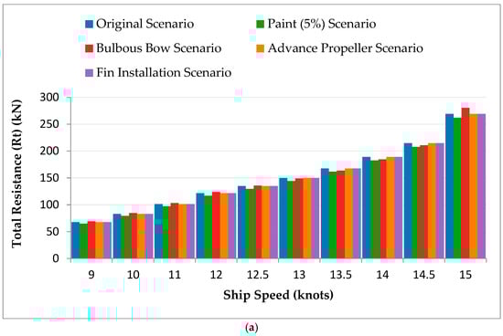
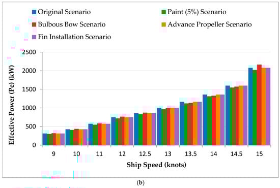
Figure 2.
(a). Total Resistance (Rt) vs. Ship Speed for Different Scenarios (Excl. Combined). (b). Adequate Power (Pe) vs. Ship Speed for Different Scenarios (Excl. Combined).
The Advanced Propeller and Fin (2–4%) scenarios followed similar resistance trends to the baseline but with noticeable reductions. The Bulbous Bow scenario showed higher resistance at low speeds but improved efficiency at higher speeds, aligning with its established performance advantages. Figure 2b highlights effective power (Pe) requirements across scenarios, with the Original Scenario demanding the most power. The Paint (5%) and Advanced Propeller Scenarios demonstrated substantial reductions in power needs. Although the Bulbous Bow Scenario initially required more power due to increased resistance, it improved at higher speeds as wave resistance decreased.
Figure 3 illustrates the thrust required (Treq) across various scenarios, reflecting trends in resistance. The Paint (5%) Scenario showed the lowest Treq due to reduced hull resistance, while the Advanced Propeller Scenario minimized thrust needs through optimized performance. The Fin (2–4%) Scenario also reduced Treq, enhancing propulsion efficiency. The Bulbous Bow Scenario required the highest thrust at lower speeds due to increased wet surface area. However, its thrust demand decreased relative to the Original Scenario at higher speeds, reflecting benefits of wave resistance.
Figure 3.
Thrust Required (Treq) vs. Ship Speed for Different Scenarios (Excl. Combined).
The Bulbous Bow scenario required the highest thrust due to its increased wetted area, while the Advanced Propeller scenario minimized thrust needs through optimized performance. The Paint (5%) scenario also showed reduced thrust demands compared to the original, highlighting the effectiveness of improved hull coatings. These graphical results indicate that different modifications have a significant impact on the ship’s hydrodynamic performance. Scenarios focusing on drag reduction (e.g., Paint (5%) and Advanced Propeller) provided the most direct improvements in resistance, power, and thrust requirements. In contrast, the Bulbous Bow scenario shows benefits primarily at higher speeds.
The comparison between Rt, Pe, and Treq for Original, Paint (5%), Bulbous Bow, and Combined Paint and Bulbous Bow Scenarios is presented in Figure A5, Figure A6 and Figure A7 of Appendix B. The Combined Scenario had the lowest Rt, Pe, and Treq at all speeds (e.g., at 12 knots, Rt = 116.21 kN, Pe = 717.23 kW, Treq = 153.07 kN, compared to 121.61 kN, 750.69 kW, 160.02 kN for the Original). This synergy, combining Paint’s frictional resistance reduction with Bulbous Bow’s wave resistance optimization, highlights the potential for integrated modifications to enhance efficiency, particularly at higher speeds where wave-making resistance dominates.
While the Combined scenario consistently reduces fuel consumption across all speeds, the relative gain at 15 knots is modest. This indicates that although wave resistance becomes more significant at higher speeds, the synergistic effect of the combined modifications produces steady rather than sharply increasing benefits.
3.4. Evaluation of Technical Modifications Before Machine Learning
Based on the calculation and analysis presented in the previous section, including the graphical results depicted in Figure 2a,b and Figure 3, the baseline analysis (Original Scenario) revealed high energy demands and environmental impact, with Pd reaching 1174.59 kW at 90 rpm and FC at 352.99 kg/h, resulting in significant CO2 emissions. Comparatively, the Paint (5%) Improvement Scenario reduced hull resistance, leading to decreased FC (276.26 kg/h at 12 knots) and Pd (1211.81 kW), showcasing enhanced energy efficiency. Similarly, the Advanced Propeller Design improved hydrodynamic efficiency, increasing propeller efficiency (ηO) from 0.464 to 0.579 at 12 knots, reducing Pb requirements.
The Fin (2–4%) Scenario demonstrated drag reduction, lowering thrust requirements to 160.02 kN at 12 knots and improving hull efficiency (ηH). The Bulbous Bow Scenario optimized flow at the bow, achieving significant efficiency gains, with Pd dropping to 1174.59 kW and FC to 267.78 kg/h at 12 knots. The Combined Paint and Bulbous Bow Scenario further reduced FC to 260.12 kg/h at 12 knots, demonstrating synergistic efficiency gains. These modifications highlight the potential for reduced energy use and emissions through targeted design enhancements.
3.5. Comparative Analysis of Modifications
Regarding comparison scenarios related to the research, FC and CO2 emissions showed significant reductions in all modified scenarios compared to the baseline. The Paint Improvement scenario effectively lowered both metrics by reducing hull resistance. The Advanced Propeller and Fins scenarios improved efficiency, consistently lowering Pb requirements. Among all modifications, the Bulbous Bow proved the most effective, achieving consistent reductions in FC and emissions across all ship speeds. Figure 4a shows FC comparisons in different scenarios, and Figure 4b demonstrates a comparison of CO2 emissions between different scenarios as follows:
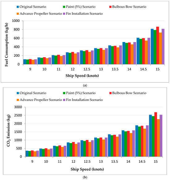
Figure 4.
(a) Comparative FC Trends for Original and Modified Scenarios (Excl. Combined). (b) CO2 Emission Trends Across Scenarios (Excl. Combined).
The Combined Paint and Bulbous Bow Scenario achieved consistent FC reductions at every speed point compared to single modifications, with cuts between 5.23% at 9 knots (108.59 kg/h) and 5.37% at 15 knots (771.04 kg/h) compared to the Original Scenario. The Combined Scenario produced 260.12 kg/h of FC at 12 knots, which was lower than the 263.48 kg/h (Paint Efficiency), 284.26 kg/h (Bulbous Bow), and 276.27 kg/h (Original). The Fin Installation and Advanced Propeller Scenarios decreased FC, but their effects were less significant. The Combined Scenario demonstrated a strong negative correlation (r = −0.99) between ship speed and relative FC reduction, indicating that efficiency gains were more significant at higher speeds. The combined effect of reduced frictional and wave-making resistance demonstrates how integrated hydrodynamic improvements can work together to achieve better results. The detailed FC comparisons across speeds are presented in Table A4 and Figure A8 of Appendix B, and CO2 emissions are illustrated in Figure A9.
Finally, it is pertinent to mention that the accuracy of the ML models was evaluated by comparing their predictions with independently computed physics-based values, serving as a validation baseline. This comparison confirmed that the models—particularly XGB and GPR—achieved high agreement with theoretical predictions, supporting the robustness of the hybrid framework.
3.6. Scenario-Specific Performance Insights
The efficiency gains across ship speeds (9 to 15 knots) are illustrated in Figure 5a,b, which show the percentage reduction in FC and thrust required (Treq) relative to the Original Scenario. Among all configurations, the Advanced Propeller achieved the largest FC reduction, ranging from 4.9% to 6.2%, due to its higher open water efficiency (ηₒ = 0.579), which represents a 24.78% improvement over the baseline propeller (ηₒ = 0.464). This improvement is calculated as follows: (0.579 − 0.464)/0.464 × 100.
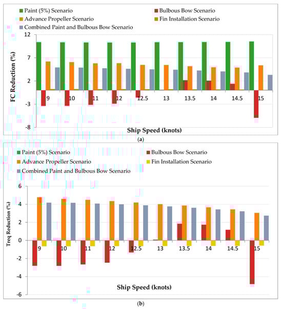
Figure 5.
(a) FC Reduction Across Speeds. (b) Treq Reduction Across Speeds.
The Combined Scenario (Paint + Bulbous Bow) followed, yielding consistent FC reductions of 3.3% to 4.9%, while the Paint (5%) Scenario achieved reductions of 10.3% to 10.5% across all speeds. Although the Paint Scenario models only a 5% reduction in the frictional resistance coefficient (CF), its impact on fuel consumption is amplified at higher speeds where resistance increases non-linearly.
In contrast, the Fin Installation Scenario produced negligible FC savings (0.06% to 0.26%). The Bulbous Bow Scenario exhibited mixed results: at low speeds (e.g., 9 knots), fuel consumption increased by 3.36% due to greater wetted surface area and added resistance. However, at mid-range speeds (e.g., 13.5 knots), it reduced FC by 2.17%, demonstrating its benefit in mitigating wave resistance. At 15 knots, however, fuel consumption increased again by 5.93%, indicating diminishing returns at higher speeds.
Moreover, Figure 5b presents the Treq changes. The Combined Scenario showed the greatest Treq reduction (2.7% to 4.2%), followed by the Advanced Propeller (3.0% to 4.8%). The Paint Scenario yielded no change in Treq (0%), while the Fin Scenario slightly increased Treq by 0.58% to 0.65%. The Bulbous Bow Scenario increased Treq at lower speeds (e.g., 2.81% increase at 9 knots) but produced reductions at higher speeds (e.g., 1.83% decrease at 13.5 knots and 4.83% decrease at 15 knots), reflecting its speed-dependent hydrodynamic performance.
The efficiency of open water (η_O) plays a crucial role, especially in the Advanced Propeller Scenario, where higher η_O reduces Pd and FC, especially at higher speeds. However, η_O remains constant for Paint, Bulbous Bow, Fin, and Combined Scenarios (η_O = 0.464), so η_O increase is excluded from Figure 5a,b to avoid uninformative zero bars, with FC and Treq reductions providing more precise insights. These modifications show that hydrodynamic improvements can reduce FC and CO2 emissions, but their effects depend on operating conditions. The Combined Scenario performs better than individual modifications, as explained in Section 3.2.
3.7. Comparative Analysis of Machine Learning Model Performance
The evaluation of ML models—Support Vector Regression (SVR), Gaussian Process Regression (GPR), Random Forest (RF), Extreme Gradient Boosting (XGB), and Neural Networks (NN)—takes place before and after MC simulations to assess their prediction capabilities for FC and CO2 emissions across ship modification scenarios, including Paint, Advanced Propeller, and the Combined Scenario, which incorporates all optimizations. The selected graphs present the most important findings, while Table A12 in Appendix D provides detailed results for the original and paint scenarios and ML models. The following observations reveal the effects of applying MC simulation for dataset augmentation and its impact on model accuracy.
The XGB model generates FC predictions for the Combined Scenario, which are compared to the Original Scenario in Figure 6. XGB produced highly accurate predictions for the 771.04 kg/h FC at 15 knots without MC simulation because it matched the actual value of 771.04 kg/h. The XGB model achieved near-perfect alignment after MC simulation with a prediction of 771.04 kg/h while demonstrating better fuel efficiency than the Original Scenario’s 814.84 kg/h.
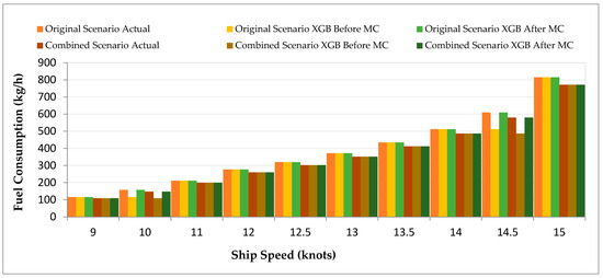
Figure 6.
FC Comparison Before and After ML (XGB) and After ML with MC for Combined Scenario.
The GPR results for FC in the Advanced Propeller Scenario are shown in Figure 7. The original calculations showed better alignment with GPR than SVR before MC simulation (e.g., FC of 638.46 kg/h at 15 knots vs. actual 729.31 kg/h). The accuracy of GPR improved substantially after MC simulation to reach 633.07 kg/h, especially in cases such as the Advanced Propeller Coefficients, demonstrating GPR’s capability to handle intricate data patterns.
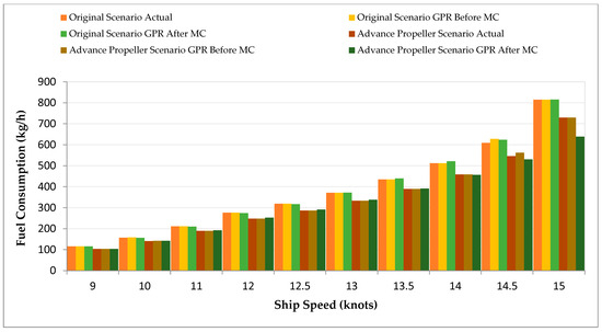
Figure 7.
FC Comparison Before and After ML (GPR) and After ML with MC for Advanced Propeller Scenario.
The evaluation of RF through FC reveals its performance, as shown in Figure 8. The predictive performance of RF was acceptable before MC simulation, but it performed worse than GPR and XGB (e.g., 772.47 kg/h at 15 knots vs. 787.84 kg/h in Paint). MC simulation yielded moderate improvements in RF, resulting in predictions of 682.38 kg/h, indicating its potential for more straightforward applications.
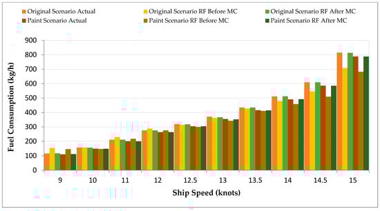
Figure 8.
FC Comparison Before and After ML (RF) and After ML with MC for Paint Modification Scenario.
The Paint Modification Scenario in Figure 9 shows XGB as the top-performing model. XGB produced highly accurate predictions without MC simulation because its results matched the original values precisely (e.g., 788.36 kg/h at 15 knots vs. 787.84 kg/h). The model achieved near-perfect alignment in Paint Modifications and the Combined Scenario after undergoing MC simulation.
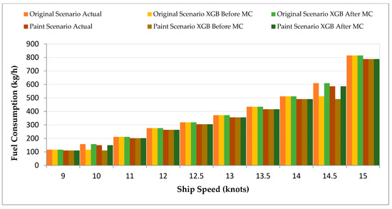
Figure 9.
FC Comparison Before and After ML (XGB) and After ML with MC for Paint Modification Scenario.
The performance of NN is shown in Figure 10. NN showed some improvement after MC simulation, but its predictions were not consistent across different scenarios (e.g., FC of 806.87 kg/h at 15 knots vs. actual 771.04 kg/h in Combined). This variability indicates the need for more optimization and hyperparameter tuning when using NN for this application.
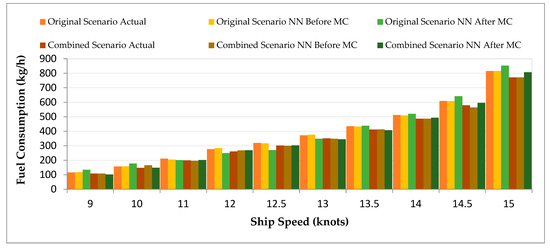
Figure 10.
FC Comparison Before and After ML (NN) and After ML with MC for Combined Scenario.
Figure 11 shows the predicted FC using SVR. SVR predictions were far from the original physics-based calculations without MC simulation, especially at higher speeds (e.g., FC of 327.78 kg/h at 15 knots vs. actual 771.04 kg/h in Combined). However, after MC simulation, the augmented dataset helped to reduce these discrepancies but only to a limited extent (e.g., FC of 334.31 kg/h), indicating limited improvement in SVR’s predictive capabilities.
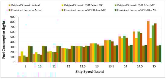
Figure 11.
FC Comparison Before and After ML (SVR) and After ML with MC for Combined Scenario.
a. CO2 Emissions Analysis
The Advanced Propeller Scenario CO2 emission predictions from GPR are presented in Figure 12. The model provided accurate results before MC simulation (e.g., CO2 1949.72 kg at 15 knots vs. actual 2268.14 kg) and achieved major improvements after MC (e.g., CO2 of 1968.83 kg), resulting in reliable emission predictions.
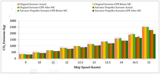
Figure 12.
CO2 Emission Comparison Before and After ML (GPR) and After ML with MC for Advanced Propeller Scenario.
The analysis of RF’s CO2 emission predictions appears in Figure 13. The model achieved better results after MC simulation, but its performance remained less reliable than GPR and XGB (e.g., CO2 of 2122.20 kg at 15 knots vs. actual 2450.20 kg in Paint).
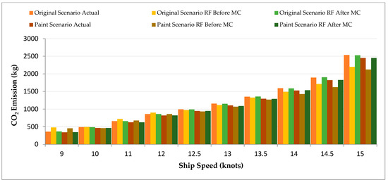
Figure 13.
CO2 Emission Comparison Before and After ML (RF) and After ML with MC for Paint Modification Scenario.
The XGB model demonstrates outstanding accuracy in its CO2 predictions for the Combined Scenario, as shown in Figure 14 (e.g., CO2 of 2397.93 kg at 15 knots vs. actual 2397.93 kg), representing a substantial decrease from the Original Scenario’s 2534.16 kg. The model delivered superior results across all scenarios, especially when making exact predictions such as Paint Modifications (e.g., CO2 of 2454.72 kg at 15 knots vs. actual 2450.20 kg post-MC).
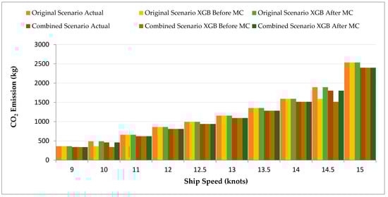
Figure 14.
CO2 Emission Comparison Before and After ML (XGB) and After ML with MC for Combined Scenario.
The SVR model failed to reach acceptable accuracy levels at both pre- and post-MC simulation stages (e.g., CO2 of 1016.35 kg at 15 knots vs. actual 2397.93 kg before MC, improving to 1022.88 kg post-MC in Combined), indicating its unsuitability for such applications. NN’s CO2 predictions improved after MC simulation but remained inconsistent (e.g., CO2 of 2510.53 kg at 15 knots vs. actual 2397.93 kg in Combined), indicating a need for further enhancements to achieve robust predictions. The detailed results of all simulations, including all scenarios (Original, Paint, Fin, Advanced Propeller, Bulbous Bow, and Combined) and ML models after MC sampling, are presented in Table A14 of Appendix D, providing a comprehensive reference for model performance.
MC simulation produced positive effects across all models, improving the match between predicted values and the original physics-based calculations. The XGB and GPR models proved to be the most reliable, producing accurate predictions for FC and CO2 emissions, particularly in the Combined Scenario, demonstrating the potential of integrated ship modifications to enhance efficiency and reduce emissions. The strength of ML methods lies in their ability to capture non-linear relationships and adapt to dynamic operational conditions, as demonstrated by real-time input simulations (e.g., engine power: 870 kW, ship speed: 12.7 knots, Section 4.3), which physics-based models alone struggle to model accurately due to their reliance on static assumptions. In contrast, SVR and NN demonstrated limited effectiveness, even after the dataset was augmented through MC simulation. The following section delves deeper into quantitative evaluations using Mean Squared Error (MSE) plots to comprehensively assess the models’ predictive accuracy and identify the most effective approach for specific scenarios.
The synthetic data points produced by MC simulations underwent validation through physics-based calculations of a selected subset of augmented samples. The SVR model evaluated one synthetic sample for each original data point to verify that the generated values for thrust (T), Pd, and FC stayed within the oil tanker specifications (Appendix A, Table A1). The Paint scenario at 14.5 knots receives validation through Table 2, which shows the original FC value against SVR model predictions before and after MC augmentation. The MC-augmented prediction shows substantial improvement, which verifies the physical accuracy of synthetic data. The validation samples for Advanced Propeller, Bulbous Bow, Combined, and Fin scenarios are presented in Appendix B, Table A5. The SVR model trained on the augmented dataset produced FC predictions with an R2 score of 0.95 across all scenarios, demonstrating substantial predictive accuracy and low overfitting, as the model performs well on new test data.
Table 2.
Sample Validation of Augmented Data for Paint Scenario (14.5 knots).
b. Model Evaluation Based on MSE Metrics
SVR consistently showed high MSE and RMSE values before and after MC simulations. Despite significantly reducing errors post-simulation, SVR’s values remained relatively high compared to other models, indicating its limited suitability for accurate predictions in this application. Specifically, in the “Bulbous Bow” scenario, RMSE for FC decreased from approximately 135.70 before MC to 33.99 after MC, demonstrating improvement but still lagging behind other models in terms of accuracy. The Combined Scenario showed similar patterns for SVR, with high MSE values before MC simulation that decreased significantly after MC but remained less competitive than the XGB and GPR models. This further underscores SVR’s challenges in achieving high precision across diverse scenarios. Table 3 shows SVR’s performance across all scenarios, emphasizing its relative lack of reliability. Mean MSE and RMSE values for FC predictions across all models are provided in Appendix D, Table A13.
Table 3.
MSE Performance for FC and RMSE Performance for CO2 Emissions of SVR Across Scenarios.
XGB and GPR emerged as the most accurate models. XGB demonstrated low MSE values after MC simulations across all scenarios, even reaching zero MSE in some cases, indicating a perfect fit for those conditions.
In scenarios such as “Paint (5%)” and “Bulbous Bow,” XGB’s RMSE values effectively became zero after MC simulations, highlighting its robustness and ability to handle variability. This is further described in Figure 15 and 16, which compares XGB’s performance against GPR, RF, and SNN. GPR also demonstrated strong predictive capabilities, particularly in the “Advanced Propeller” scenario, where it outperformed XGB in terms of MSE and RMSE. This suggests that GPR can be advantageous in specialized contexts with more complex underlying dynamics. Overall, GPR maintained low RMSE values, particularly in scenarios with increased complexity, demonstrating its flexibility and adaptability.
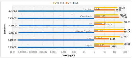
Figure 15.
MSE performance comparison of XGB, GPR, RF, and SNN for FC across scenarios.
RF and SNN models performed moderately well but did not achieve the same levels of accuracy as XGB or GPR. While demonstrating error reduction after MC simulations, the RF model still had higher MSE values than the top-performing models. For instance, in the “Bulbous Bow” scenario, MSE for RF dropped from approximately 2512.84 to 3.63 after MC simulations. Yet, RMSE remained comparatively high at 1.90, indicating a need for more generalizability. This trend was evident across multiple scenarios, suggesting that RF is less consistent in reducing prediction errors when compared to GPR and XGB. SNN improved after MC simulations, with reduced MSE values across many scenarios. However, their performance could have been better. In particular, in the “Fin (2–4%)” scenario, RMSE for FC decreased from approximately 10.92 to 8.04, indicating improvement; however, it still falls short of the results achieved with GPR or XGB. The inconsistencies in SNN performance render it less reliable for predictions that require high accuracy across varying conditions. Figure 15 highlights the comparative performance of XGB, GPR, RF, and SNN models, illustrating SNN’s moderate yet inconsistent improvements. Detailed MSE performance for the other models is available in Appendix D, Table A14.
It is relevant to note that the MSE values shown may reflect differences in internal scaling between models. While the relative performance trends are valid, the absolute values should be interpreted with caution.
c. Detailed Scenario-Based Analysis
Evaluating different scenarios provides a more granular view of each model’s behavior under varying conditions. Below is a detailed discussion of model performance for specific scenarios:
- i.
- Original Scenario: This scenario served as a baseline for comparison. XGB and GPR both demonstrated the best performance, achieving low MSE and RMSE values, especially after MC simulations. While showing error reductions post-simulation, the SVR model still had high RMSE values of approximately 27.68, indicating its lack of precision.
- ii.
- Paint (5%) Scenario: In this scenario, XGB continued to demonstrate excellent performance, with an MSE value of zero post-simulation, indicating that the model effectively generalized the new conditions introduced by the paint modification. GPR also showed strong performance, while RF and SNN showed moderate levels of error reduction.
- iii.
- Advanced Propeller Scenario: The Advanced Propeller scenario demonstrated GPR’s ability to handle complex modifications. GPR achieved the lowest MSE and RMSE compared to other models, making it the best performer in this context. XGB also performed well, but not as consistently as GPR, particularly before the MC simulation.
- iv.
- Fin (2–4%) Scenario: In this scenario, XGB and GPR were again the most effective, while SNN showed improvements but still lagged. The RF model exhibited moderate improvements but failed to match the performance levels of XGB and GPR. This scenario highlighted the limitations of RF and SNN in scenarios with minor, more nuanced changes.
- v.
- Bulbous Bow Scenario: In the Bulbous Bow scenario, XGB and GPR maintained high performance, with XGB achieving perfect accuracy (MSE of zero post-simulation). SVR showed improvements but had higher error levels, making it the least effective for this scenario. SNN performed inconsistently, suggesting sensitivity to the modifications in this particular scenario.
- vi.
- Combined Scenario: The Combined Scenario tested the models’ ability to generalize across diverse conditions by integrating multiple modifications. XGB achieved near-zero MSE, reinforcing its robustness, while GPR maintained low MSE values, though higher than XGB’s. RF performed moderately, with MSE values lower than those of SNN, which showed higher errors, indicating inconsistent performance in complex scenarios.
3.8. Implementation of the XGB Model and Summary of Results
Building upon the comparative analysis of ML models, where XGB demonstrated superior predictive performance, this section details the implementation of the XGB model and summarizes the key results obtained. By integrating the XGB model into the hybrid framework, the authors aimed to enhance predictive accuracy for FC and CO2 emissions under various operational scenarios. A single XGB model was trained on a combined dataset from all scenarios (Original, Paint, Advanced Propeller, Fin, Bulbous Bow, Combined) to enable flexible predictions for diverse ship configurations.
The following subsections discuss the user interface development, visualization, and comparative analysis of predictions across different scenarios; key insights derived from the results; quantitative evaluation of the model’s predictions; and an assessment of XGB’s overall performance in capturing complex maritime operational dynamics.
- i.
- Visualization and Comparative Analysis
Predictions were visualized across a range of ship speeds (9 to 15 knots) using a single model trained on all scenarios. Graphs illustrated the relationship between ship speed and predicted metrics:
- Fuel Consumption: The bar chart demonstrates how the combined model predicts FC (after MC augmentation) at different speeds, exhibiting similar FC reduction patterns to efficiency-based scenarios such as “Advanced Propeller” and “Bulbous Bow” at higher speeds.
- CO2 Emissions: The bar chart of CO2 emissions mirrored the FC pattern, showing reduced emissions in configurations that matched the “Advanced Propeller” and “Fin (2–4%)” scenarios.
- MC-augmented: The MC-augmented predictions matched the scenario-specific trends, demonstrating the model’s ability to capture parameter effects accurately. The visualization illustrates how different configurations align with the aggregated scenario trends, enabling practical interpretation.
- ii.
- Key Insights
- Fuel Consumption: The combined model captured efficiency gains consistent with scenarios like “Advanced Propeller” at higher speeds, where propeller efficiency improvements reduce FC. The “Bulbous Bow” scenario also improved FC significantly at high speeds by reducing wave resistance.
- CO2 Emissions: The model predicted CO2 emissions through efficiency-driven scenarios such as “Advanced Propeller” and “Fin (2–4%)”, which matched expected hydrodynamic improvements.
The XGB model demonstrated its ability to handle operational condition variability, thus proving its effectiveness for real-world deployment. The combined FC and CO2 prediction trends are shown in Figure 16, with user input overlay.
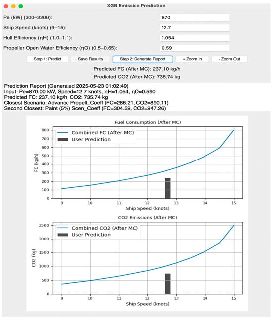
Figure 16.
Combined FC and CO2 prediction across speeds with sample parameters input.
- iii.
- Quantitative Evaluation of Predictions
The XGB model predicted an FC of 237.10 kg/h and CO2 emissions of 735.74 kg after MC augmentation, using the following sample operational inputs: engine power (Pe: 870 kW), ship speed (12.7 knots), hull efficiency (ηH: 1.054), and propeller efficiency (ηO: 0.590). The configuration shows the closest match to the “Advanced Propeller” scenario (FC: 286.21 kg/h, CO2: 890.11 kg) followed by the “Paint (5%)” scenario (FC: 304.59 kg/h, CO2: 947.26 kg). The setup with its high propeller efficiency (ηO = 0.590) benefits from efficiency improvements that are similar to those in the “Advanced Propeller” scenario, which focuses on enhanced propeller design. The predicted values are lower than expected (FC: 284.26 kg/h, CO2: 884.04 kg), which may indicate underestimation, possibly due to the model’s generalization across diverse scenarios. To achieve further reductions in FC and CO2, the model suggests improvements similar to the “Advanced Propeller” scenario, such as adopting advanced propeller technologies to enhance ηO.
- iv.
- Evaluation of XGB Model Performance
XGB demonstrated superior performance to other ML models, such as RF and GPR, which struggled with overfitting or underfitting in specific scenarios. Its ability to capture non-linear relationships between features and robustness to scenario variations made it the most effective model for predicting FC and CO2 emissions. With hyperparameters optimized (e.g., 100 estimators for a balance of efficiency and accuracy), XGB effectively generalized across operational scenarios, providing reliable predictions.
4. Discussion
This study’s comprehensive evaluation of technical modifications and ML approaches provides significant insights into enhancing ship efficiency and reducing emissions for maritime operations. Integrating physics-based calculations with advanced ML models, supplemented by data augmentation through MC simulations, has demonstrated the potential for accurate and reliable predictions of FC and CO2 emissions under various operational scenarios. The study trains a single XGB model on a combined dataset from all scenarios to enable flexible predictions for assumption-defined configurations, which addresses real-world scenarios where ship designs may not align with predefined modifications.
4.1. Effectiveness of Technical Modifications
The analysis of different technical modifications before the application of ML models highlighted the tangible benefits of targeted design enhancements:
- Advanced Propeller Design: This modification consistently improved thrust requirements and effective power across varying speed ranges. By increasing the propeller’s open water efficiency () from 0.464 to 0.579 at 12 knots, it effectively reduced energy consumption, particularly at higher speeds. This demonstrates the propeller’s ability to enhance hydrodynamic efficiency and operational performance under diverse conditions.
- Paint Efficiency Improvement (5% Reduction): The application of advanced hull coatings reduced the frictional resistance coefficient (CF), leading to decreased hull resistance. This resulted in lower FC (e.g., 276.26 kg/h at 12 knots) and Pd, showcasing enhanced energy efficiency through drag reduction. The findings validate the benefits of high-quality hull coatings in improving fuel economy.
- Fin Installation: By enhancing thrust by 2% and improving the wake fraction by 4%, fins lowered thrust requirements () to 160.02 kN at 12 knots and improved hull efficiency (ηH). This modification contributed to overall operational efficiency, highlighting the potential of appendages in optimizing propulsion.
- Bulbous Bow Addition: The bulbous bow scenario optimized flow at the bow, achieving the most significant efficiency gains, particularly at higher speeds. Although it increased wetted surface area and resistance at lower speeds, the bulbous bow reduced wave-making resistance at higher speeds, aligning with established naval architecture principles. This modification reduced FC to 267.78 kg/h at 12 knots and demonstrated its effectiveness for vessels operating at moderate to high speeds.
4.2. Impact of Data Augmentation with Monte Carlo Simulations
The use of MC simulations for data augmentation has shown significant efficacy in enhancing the performance of ML models. This method enhanced the dataset by introducing controlled variability and modeling real-world uncertainties, enabling the models to more effectively discern the intricate correlations between operational factors and target variables. Data augmentation significantly mitigated overfitting, enabling models such as XGB and GPR to generalize more proficiently across various contexts. After data augmentation, the decrease in MSE and RMSE values underscored the significant improvement in predictive accuracy, particularly for models susceptible to data fluctuation. The XGB model achieved better generalization through the combined dataset approach with 3× MC augmentation, which enabled it to predict FC and CO2 emissions for various user configurations while minimizing the overfitting risk that scenario-specific models exhibited.
The hybrid model is built on a succession of controlled simplifications, yet it does provide an organized and repeatable foundation. The authors did not dynamically model environmental circumstances, including the state of the sea, wind forces, uneven loads, and long-term impacts of hull fouling. Instead, the authors employed idealized hydrodynamic characteristics. Marine biofouling can make hull coatings and other treatments less effective over time, which can have a big effect on resistance and fuel use.
The authors also used constant BSFC and transmission efficiency values to provide an idea of how the engine will perform in different operational modes. Future versions of the model will try to include these changing, real-world aspects by using sensor-based empirical data, time-dependent degradation models, and probabilistic simulations that better show how the environment changes.
4.3. Practical Implications and Applications
The findings of this study offer significant practical implications for reducing FC and CO2 emissions in oil tanker operations, with applicability extending to other similar vessels. The XGB model, identified as the most accurate predictor of FC and CO2 emissions (Section 3.5), provides a reliable tool for forecasting operational performance across diverse conditions, enabling data-driven decision-making for tanker operators and designers.
For example, a simulated operational scenario with Pe = 870 kW, 12.7 knots, ηH = 1.054, and ηO = 0.590 resulted in predicted FC of 237.10 kg/h and CO2 emissions of 735.74 kg, which is close to the Advanced Propeller scenario, indicating that adopting advanced propeller designs could optimize efficiency (Section 3.8). The Advanced Propeller scenario achieved the most significant FC reduction (e.g., 729.31 kg/h at 15 knots compared to 814.84 kg/h for the Original scenario), followed by the Combined scenario (771.04 kg/h), which demonstrates effective modifications for enhancing fuel efficiency and reducing emissions.
Ship operators can utilize these insights to adjust operational parameters, such as selecting optimal speeds or installing advanced propellers, to reduce emissions. Designers can use scenario comparisons to determine which modifications should be prioritized, such as improving propeller efficiency or investigating hybrid configurations during ship design to achieve sustainability goals. The model’s precise emission projections enable the achievement of global sustainability targets while supporting environmental preservation and compliance with international regulations. The model’s robustness results from MC data augmentation (Section 2.2) and validation at 8 knots for minimal FC (Appendix B, Table A6), which enables its application to other oil tankers to expand its maritime sustainability impact. The study does not address the monetary aspects of modifications, but the technical performance data would allow stakeholders to perform cost-benefit analyses.
This study assumes a constant BSFC of 200 g/kWh for simplicity; however, actual engine performance fluctuates with load. Marine engines generally achieve optimal efficiency at 75–85% of Maximum Continuous Rating (MCR). In contrast, operating at lower loads (<50% MCR) may lead to increased Brake Specific Fuel Consumption (BSFC) due to suboptimal combustion, higher auxiliary power requirements, and increased oil consumption. Future model enhancements should integrate variable BSFC profiles and investigate the potential of machine learning to identify optimal operating points that reconcile propulsion improvements with slow steaming and energy efficiency goals.
This study assumes a constant transmission efficiency of 96.5%, representing a simplified model of a direct-drive shaft system typically employed in medium-sized oil tankers. This value, although supported by high-efficiency propulsion configurations with minimal mechanical losses, fails to account for the variability introduced by differing propulsion layouts or operating conditions. Transmission efficiency is influenced by factors such as shaft speed, load, and the incorporation of reduction gears or intermediate couplings. Future developments of the model should incorporate a load-dependent transmission efficiency profile and a modular representation of the propulsion chain to enhance realism and predictive accuracy.
5. Conclusions
The research developed a physics-based ML hybrid system to forecast oil tanker FC and CO2 emissions through hydrodynamic modeling and sophisticated ML algorithms, advancing maritime sustainability. The study trained one XGB model to predict various ship configurations through a combined dataset from Original, Paint, Advanced Propeller, Fin, Bulbous Bow, and Combined scenarios, which handles real-world design and operational variations. The research aimed to assess technical modifications for reducing FC and CO2 emissions while developing an ML model that could be applied to other oil tankers. The XGB model achieved superior performance compared to Support Vector Regression, Gaussian Process Regression, Random Forest, and Shallow Neural Network models by demonstrating high predictive accuracy when validated against physics-based calculations. The Advanced Propeller scenario produced the largest FC reduction, followed by the Combined scenario, indicating substantial potential for reducing CO2 emissions.
The model’s predictions enabled scenario comparisons, which provided practical insights into how operators should prioritize advanced propeller designs or hull coatings to maximize efficiency, thereby helping operators optimize vessel operations and designers achieve sustainability targets. The research results directly inform operational planning and design choices through simulated predictions (e.g., a flow rate of 237.10 kg/h for specific inputs, Section 3.8), providing practical utility without requiring an interface. The research supports IMO decarbonization targets through its data-driven maritime efficiency solution.
The research has made progress, but it faces two main challenges and limitations: the initial dataset is small, necessitating the use of MC data augmentation, and the predictions are sometimes underestimated, which could be improved by incorporating features such as paint properties or wave resistance. Future research should expand empirical datasets to include diverse ship types, optimize models such as Shallow Neural Networks, and explore deep learning techniques. Real-time sensor data integration would enable dynamic monitoring, thereby enhancing operational efficiency. The development of innovative, sustainable ship performance solutions that meet global environmental regulations requires transdisciplinary collaboration between naval architects, oceanographers, and AI experts.
Future studies should focus on integrating real-time operational data from multiple vessel types to validate and enhance model generalizability. Incorporating advanced hybrid algorithms with adaptive learning capabilities could further improve predictive accuracy under variable marine conditions. Additionally, exploring environmental and economic trade-offs of combined technical modifications across different ship classes would broaden the applicability of this framework. Lastly, deeper integration of sensor-based IoT systems may support continuous emissions monitoring and optimization.
Author Contributions
Conceptualization; methodology; software; validation; formal analysis; investigation; resources; data curation; writing—original draft preparation; writing—review and editing; visualization; supervision; project administration H.R.S.M., S.B.I.-Z. and C.L.G.-R.; validation M.R.Z. All authors have read and agreed to the published version of the manuscript.
Funding
There is not any funding resources available.
Data Availability Statement
The original contributions presented in this study are included in the article material. Further inquiries can be directed to the author.
Conflicts of Interest
The authors declare no conflicts of interest.
Appendix A. Ship Characteristics and Test Results
Table A1.
Examined oil tanker dimensions and main characteristics.
Table A1.
Examined oil tanker dimensions and main characteristics.
| Parameter | Symbol | Unit | Value |
|---|---|---|---|
| Length overall | LOA | (m) | 100 |
| Length between perpendiculars | LBP | (m) | 98.1 |
| Waterline length | LWL | (m) | 100 |
| Wetted length | LWS | (m) | 100 |
| Breadth (at wl) | B | (m) | 16.6 |
| Draught (midship) | T | (m) | 6.5 |
| Draught (AP) | TA | (m) | 6.5 |
| Draught (FP) | TF | (m) | 6.5 |
| Displacement volume | ∇ | (m3) | 7771.6 |
| Displacement | ∆ | (ton) | 7965.9 |
| Wetted surface area | AWS | (m2) | 2350 |
| The surface area of the rudder(s) | AR | (m2) | 58.5 |
| Total surface area of appendages | AA | (m2) | 41 |
| Bulbous sectional area | AB | (m2) | 0 |
| Centre of bulbous sectional area | HB | (m) | 0 |
| Transom area | AT | (m2) | 1.9 |
| Centre of the transom area | HT | (m) | 6.25 |
| Block coefficient | CB | - | 0.72 |
| Prismatic coefficient | CP | - | 0.73 |
| Midship area coefficient | CM | - | 0.986 |
| Waterplane area coefficient | CWP | - | 0.862 |
| Longitudinal center of buoyancy | LCB | (m) (from AP) | 48.1 |
| Longitudinal center of floatation | LCF | (m) (from AP) | 45.12 |
| Service speed | - | knots | 13.5 |
| Propeller diameter | - | M | 4 |
| Number of blades | - | - | 4 |
| Blade area ratio | - | - | 0.4 |
| Pitch/diameter ratio | - | m | 0.74 |
| Transmission efficiency | - | - | 0.965 |
| Water density | - | kg/m3 | 1025 |
| Water temperature | - | °C | 15 |
| Kinematic viscosity | v | m2/s | 1.18831 10 −3 |
| Brake Specific Fuel Consumption | BSFC | g/kWh | 200 |
Table A2.
Oil Tanker Ship Model- Examined Test Results.
Table A2.
Oil Tanker Ship Model- Examined Test Results.
| Ship Speed (Knots) | Wave Resistance Coefficient 1000 (Without Bulbous Bow) | Wave Resistance Coefficient 1000 (with Bulbous Bow) | Thrust Deduction | Wake Fraction | Relative Rotative Efficiency |
|---|---|---|---|---|---|
| 6 | 0.44 | 0.462 | 0.247 | 0.289 | 1.012 |
| 7 | 0.461 | 0.479 | 0.245 | 0.287 | 1.012 |
| 8 | 0.451 | 0.465 | 0.245 | 0.287 | 1.012 |
| 9 | 0.435 | 0.444 | 0.244 | 0.286 | 1.012 |
| 10 | 0.439 | 0.448 | 0.243 | 0.285 | 1.012 |
| 10.5 | 0.457 | 0.462 | 0.243 | 0.284 | 1.012 |
| 11 | 0.49 | 0.495 | 0.242 | 0.283 | 1.012 |
| 11.5 | 0.538 | 0.538 | 0.240 | 0.281 | 1.012 |
| 12 | 0.604 | 0.574 | 0.238 | 0.279 | 1.012 |
| 12.5 | 0.692 | 0.623 | 0.236 | 0.276 | 1.012 |
| 13 | 0.805 | 0.684 | 0.234 | 0.272 | 1.012 |
| 13.5 | 0.953 | 0.829 | 0.231 | 0.268 | 1.012 |
| 14 | 1.141 | 1.027 | 0.229 | 0.264 | 1.012 |
| 14.5 | 1.385 | 1.385 | 0.226 | 0.260 | 1.012 |
| 15 | 1.701 | 1.786 | 0.223 | 0.255 | 1.012 |
Table A3.
Propulsion Open Water Efficiency for Different Types of Propellers.
Table A3.
Propulsion Open Water Efficiency for Different Types of Propellers.
| Original Propeller | Advanced Propeller | |||
|---|---|---|---|---|
| J | Kt | 10⋅Kq | Kt | 10⋅Kq |
| 0.05 | 0.2993 | 0.3696 | 0.3151 | 0.35196 |
| 0.1 | 0.2882 | 0.359 | 0.3034 | 0.34191 |
| 0.15 | 0.2762 | 0.3479 | 0.2907 | 0.33129 |
| 0.2 | 0.2632 | 0.336 | 0.277 | 0.32002 |
| 0.25 | 0.2493 | 0.3234 | 0.2624 | 0.30803 |
| 0.3 | 0.2346 | 0.31 | 0.2469 | 0.29523 |
| 0.35 | 0.219 | 0.2956 | 0.2305 | 0.28155 |
| 0.4 | 0.2026 | 0.2803 | 0.2133 | 0.26692 |
| 0.45 | 0.1855 | 0.2638 | 0.1953 | 0.25126 |
| 0.5 | 0.1678 | 0.2462 | 0.1766 | 0.2345 |
| 0.55 | 0.1492 | 0.2274 | 0.1571 | 0.21656 |
| 0.6 | 0.1302 | 0.2072 | 0.137 | 0.19735 |
| 0.65 | 0.1105 | 0.1857 | 0.1163 | 0.17682 |
| 0.7 | 0.0903 | 0.1626 | 0.095 | 0.15488 |
| 0.75 | 0.0694 | 0.138 | 0.0731 | 0.13145 |
| 0.8 | 0.0482 | 0.1118 | 0.0507 | 0.10646 |
| 0.85 | 0.0264 | 0.0838 | 0.0278 | 0.07983 |
Appendix B. Propeller Performance Charts

Figure A1.
Kt vs. J for original propeller with quadratic fit (R2 = 1.000).

Figure A2.
Kq vs. J for original propeller with quadratic fit (R2 = 1.000).

Figure A3.
Kt vs. J for advanced propeller with quadratic fit (R2 = 1.000).

Figure A4.
Kq vs. J for advanced propeller with quadratic fit (R2 = 1.000).

Figure A5.
Total resistance (Rt) vs. ship speed including combined scenario.

Figure A6.
Effective power (Pe) vs. ship speed including combined scenario.

Figure A7.
Thrust required (Treq) vs. ship speed including combined scenario.

Figure A8.
FC vs. ship speed including combined scenario.

Figure A9.
CO2 emission vs. ship speed including combined scenario.
Table A4.
Combined Paint and Bulbous Bow Scenario Parameters.
Table A4.
Combined Paint and Bulbous Bow Scenario Parameters.
| Ship Speed (knots) | Rt (kN) | Pe (kW) | Treq (kN) | FC (kg/h) | CO2 Emission (kg) |
|---|---|---|---|---|---|
| 9 | 64.54 | 298.91 | 85.45 | 108.59 | 337.71 |
| 10 | 79.02 | 406.47 | 104.51 | 147.58 | 459.08 |
| 11 | 96.68 | 547.37 | 127.60 | 199.03 | 619.18 |
| 12 | 116.21 | 717.23 | 153.07 | 260.12 | 808.97 |
| 12.5 | 129.01 | 829.45 | 169.36 | 301.54 | 937.79 |
| 13 | 143.87 | 961.24 | 188.28 | 351.13 | 1092.01 |
| 13.5 | 161.23 | 1119.50 | 210.34 | 411.98 | 1281.26 |
| 14 | 181.84 | 1309.58 | 236.62 | 486.46 | 1512.90 |
| 14.5 | 206.82 | 1542.61 | 268.74 | 579.32 | 1801.67 |
| 15 | 260.44 | 2009.38 | 335.85 | 771.04 | 2397.93 |
Table A5.
Additional Validation Samples for Augmented Data at 14.5 knots.
Table A5.
Additional Validation Samples for Augmented Data at 14.5 knots.
| Scenario | Data Type | Fuel Consumption (FC, kg/h) |
|---|---|---|
| Advanced Propeller | Original (Physics-Based) | 545.6961681 |
| Neural Network (Before MC) | 559.4786360 | |
| Neural Network (After MC) | 529.9805960 | |
| Bulbous Bow | Original (Physics-Based) | 600.5953901 |
| Random Forest (Before MC) | 527.8524522 | |
| Random Forest (After MC) | 577.0773365 | |
| Combined | Original (Physics-Based) | 579.3200000 |
| XGB (Before MC) | 486.4600525 | |
| XGB (After MC) | 579.3199463 | |
| Fin | Original (Physics-Based) | 608.2600070 |
| GPR (Before MC) | 615.8368798 | |
| GPR (After MC) | 608.2599487 |
Table A6.
Sample Model Performance for Extrapolation at 8 knots.
Table A6.
Sample Model Performance for Extrapolation at 8 knots.
| Scenario | Data Type | Fuel Consumption (FC, kg/h) |
|---|---|---|
| Advanced Propeller | Physics-Based (Calculated) | 61.41 |
| SVR (Before MC) | 106.81 | |
| SVR (After MC) | 70.43 | |
| RF (Before MC) | 81.33 | |
| RF (After MC) | 62.03 | |
| Combined | Physics-Based (Calculated) | 63.94 |
| XGB (Before MC) | 64.27 | |
| XGB (After MC) | 64.27 | |
| GPR (Before MC) | 64.27 | |
| GPR (After MC) | 63.80 (Uncertainty: ±15) | |
| Paint | Physics-Based (Calculated) | 64.67 |
| NN (Before MC) | 64.53 | |
| NN (After MC) | 61.33 |
Note: Physics-based FC values at 8 knots are calculated using a power-law model (FC = a · V^b) fitted to 9–15 knot data (Appendix C). ML model FC predictions are extrapolated from 9-knot values using the physics-based FC ratio (8 knots/9 knots), as 8-knot ML data are unavailable. GPR uncertainty estimates indicate prediction reliability for extrapolation.
Appendix C. Detailed Calculations and Results
Table A7.
Physics-based calculations—original scenario.
Table A7.
Physics-based calculations—original scenario.
| Ship Speed (knots) | Wave Resistance Coefficient ⋅ 1000 | Thrust Deduction | Wake Fraction | Relative Rotative Efficiency | Speed m/s | Re | CF | Cv | Ct | Rt (kN) | Pe(kW) | Va (m/s) | Treq (kN) |
|---|---|---|---|---|---|---|---|---|---|---|---|---|---|
| 9 | 0.435 | 0.244 | 0.286 | 1.012 | 4.6296 | 389,595,307.6 | 0.001726671 | 0.002192872 | 0.002627872 | 67.83484964 | 314.0482199 | 3.3055344 | 89.7286371 |
| 10 | 0.439 | 0.243 | 0.285 | 1.012 | 5.144 | 432,883,675.1 | 0.001702942 | 0.002162737 | 0.002601737 | 82.91383244 | 426.5087541 | 3.67796 | 109.5295012 |
| 11 | 0.49 | 0.242 | 0.283 | 1.012 | 5.6584 | 476,172,042.6 | 0.001681896 | 0.002136008 | 0.002626008 | 101.2616638 | 572.9789987 | 4.0570728 | 133.5905855 |
| 12 | 0.538 | 0.24 | 0.281 | 1.012 | 6.1728 | 519,460,410.2 | 0.001663021 | 0.002112037 | 0.002650037 | 121.6124557 | 750.6893668 | 4.4382432 | 160.0163891 |
| 12.5 | 0.604 | 0.238 | 0.279 | 1.012 | 6.43 | 541,104,593.9 | 0.001654275 | 0.002100929 | 0.002704929 | 134.6913255 | 866.0652227 | 4.63603 | 176.7602696 |
| 13 | 0.692 | 0.236 | 0.276 | 1.012 | 6.6872 | 562,748,777.7 | 0.001645937 | 0.00209034 | 0.00278234 | 149.8513221 | 1002.085761 | 4.8415328 | 196.140474 |
| 13.5 | 0.805 | 0.234 | 0.272 | 1.012 | 6.9444 | 584,392,961.4 | 0.001637973 | 0.002080226 | 0.002885226 | 167.5756882 | 1163.712609 | 5.0555232 | 218.767217 |
| 14 | 0.953 | 0.231 | 0.268 | 1.012 | 7.2016 | 606,037,145.2 | 0.001630353 | 0.002070549 | 0.003023549 | 188.8585755 | 1360.083917 | 5.2715712 | 245.5898251 |
| 14.5 | 1.141 | 0.229 | 0.264 | 1.012 | 7.4588 | 627,681,328.9 | 0.001623051 | 0.002061275 | 0.003202275 | 214.5647195 | 1600.39533 | 5.4896768 | 278.2940591 |
| 15 | 1.701 | 0.223 | 0.255 | 1.012 | 7.716 | 649,325,512.7 | 0.001616043 | 0.002052375 | 0.003753375 | 269.1337357 | 2076.635905 | 5.74842 | 346.3754643 |
Table A8.
Physics-based calculations—paint Efficiency Scenario (5% Reduction).
Table A8.
Physics-based calculations—paint Efficiency Scenario (5% Reduction).
| Ship Speed (knots) | Wave Resistance Coefficient ⋅ 1000 | Thrust Deduction | Wake Fraction | Relative Rotative Efficiency | Speed m/s | Re | CF | Cv | Ct | Rt (kN) | Pe(kW) | Va (m/s) | Treq (kN) |
|---|---|---|---|---|---|---|---|---|---|---|---|---|---|
| 9 | 0.435 | 0.244 | 0.286 | 1.012 | 4.6296 | 389,595,307.6 | 0.001640337 | 0.002083228 | 0.002518228 | 65.00455308 | 300.945079 | 3.3055344 | 85.98485858 |
| 10 | 0.439 | 0.243 | 0.285 | 1.012 | 5.144 | 432,883,675.1 | 0.001617795 | 0.0020546 | 0.0024936 | 79.46765766 | 408.781631 | 3.67796 | 104.9770907 |
| 11 | 0.49 | 0.242 | 0.283 | 1.012 | 5.6584 | 476,172,042.6 | 0.001597801 | 0.002029208 | 0.002519208 | 97.14332675 | 549.6758001 | 4.0570728 | 128.1574232 |
| 12 | 0.538 | 0.24 | 0.281 | 1.012 | 6.1728 | 519,460,410.2 | 0.00157987 | 0.002006435 | 0.002544435 | 116.7662969 | 720.7749977 | 4.4382432 | 153.6398644 |
| 12.5 | 0.604 | 0.238 | 0.279 | 1.012 | 6.43 | 541,104,593.9 | 0.001571561 | 0.001995883 | 0.002599883 | 129.4605611 | 832.4314076 | 4.63603 | 169.8957494 |
| 13 | 0.692 | 0.236 | 0.276 | 1.012 | 6.6872 | 562,748,777.7 | 0.00156364 | 0.001985823 | 0.002677823 | 144.2222434 | 964.442986 | 4.8415328 | 188.7725699 |
| 13.5 | 0.805 | 0.234 | 0.272 | 1.012 | 6.9444 | 584,392,961.4 | 0.001556074 | 0.001976215 | 0.002781215 | 161.5346485 | 1121.761213 | 5.0555232 | 210.8807421 |
| 14 | 0.953 | 0.231 | 0.268 | 1.012 | 7.2016 | 606,037,145.2 | 0.001548836 | 0.001967021 | 0.002920021 | 182.3919873 | 1313.514136 | 5.2715712 | 237.1807377 |
| 14.5 | 1.141 | 0.229 | 0.264 | 1.012 | 7.4588 | 627,681,328.9 | 0.001541899 | 0.001958211 | 0.003099211 | 207.6590523 | 1548.887339 | 5.4896768 | 269.3372922 |
| 15 | 1.701 | 0.223 | 0.255 | 1.012 | 7.716 | 649,325,512.7 | 0.001535241 | 0.001949756 | 0.003650756 | 261.7755133 | 2019.85986 | 5.74842 | 336.9054225 |
Table A9.
Physics-based calculations—dvanced Propeller Scenario.
Table A9.
Physics-based calculations—dvanced Propeller Scenario.
| Ship Speed (knots) | Wave Resistance Coefficient ⋅ 1000 | Thrust Deduction | Wake Fraction | Relative Rotative Efficiency | Speed m/s | Re | CF | Cv | Ct | Rt (kN) | Pe(kW) | Va (m/s) | Treq (kN) |
|---|---|---|---|---|---|---|---|---|---|---|---|---|---|
| 9 | 0.435 | 0.244 | 0.286 | 1.012 | 4.6296 | 389,595,307.6 | 0.001726671 | 0.002192872 | 0.002627872 | 67.83484964 | 314.0482199 | 3.3055344 | 89.7286371 |
| 10 | 0.439 | 0.243 | 0.285 | 1.012 | 5.144 | 432,883,675.1 | 0.001702942 | 0.002162737 | 0.002601737 | 82.91383244 | 426.5087541 | 3.67796 | 109.5295012 |
| 11 | 0.49 | 0.242 | 0.283 | 1.012 | 5.6584 | 476,172,042.6 | 0.001681896 | 0.002136008 | 0.002626008 | 101.2616638 | 572.9789987 | 4.0570728 | 133.5905855 |
| 12 | 0.538 | 0.24 | 0.281 | 1.012 | 6.1728 | 519,460,410.2 | 0.001663021 | 0.002112037 | 0.002650037 | 121.6124557 | 750.6893668 | 4.4382432 | 160.0163891 |
| 12.5 | 0.604 | 0.238 | 0.279 | 1.012 | 6.43 | 541,104,593.9 | 0.001654275 | 0.002100929 | 0.002704929 | 134.6913255 | 866.0652227 | 4.63603 | 176.7602696 |
| 13 | 0.692 | 0.236 | 0.276 | 1.012 | 6.6872 | 562,748,777.7 | 0.001645937 | 0.00209034 | 0.00278234 | 149.8513221 | 1002.085761 | 4.8415328 | 196.140474 |
| 13.5 | 0.805 | 0.234 | 0.272 | 1.012 | 6.9444 | 584,392,961.4 | 0.001637973 | 0.002080226 | 0.002885226 | 167.5756882 | 1163.712609 | 5.0555232 | 218.767217 |
| 14 | 0.953 | 0.231 | 0.268 | 1.012 | 7.2016 | 606,037,145.2 | 0.001630353 | 0.002070549 | 0.003023549 | 188.8585755 | 1360.083917 | 5.2715712 | 245.5898251 |
| 14.5 | 1.141 | 0.229 | 0.264 | 1.012 | 7.4588 | 627,681,328.9 | 0.001623051 | 0.002061275 | 0.003202275 | 214.5647195 | 1600.39533 | 5.4896768 | 278.2940591 |
| 15 | 1.701 | 0.223 | 0.255 | 1.012 | 7.716 | 649,325,512.7 | 0.001616043 | 0.002052375 | 0.003753375 | 269.1337357 | 2076.635905 | 5.74842 | 346.3754643 |
Table A10.
Physics-based calculations—Fin Installation Scenario.
Table A10.
Physics-based calculations—Fin Installation Scenario.
| Ship Speed (knots) | Wave Resistance Coefficient ⋅ 1000 | Thrust Deduction | Wake Fraction | Relative Rotative Efficiency | Speed (m/s) | Re | CF | Cv | Ct | Rt (kN) | Pe(kW) | Va (m/s) | Treq (kN) |
|---|---|---|---|---|---|---|---|---|---|---|---|---|---|
| 9 | 0.435 | 0.24888 | 0.29744 | 1.012 | 4.6296 | 389,595,307.6 | 0.001726671 | 0.002192872 | 0.002627872 | 67.83484964 | 314.0482199 | 3.252571776 | 90.31160087 |
| 10 | 0.439 | 0.24786 | 0.2964 | 1.012 | 5.144 | 432,883,675.1 | 0.001702942 | 0.002162737 | 0.002601737 | 82.91383244 | 426.5087541 | 3.6193184 | 110.237233 |
| 11 | 0.49 | 0.24684 | 0.29432 | 1.012 | 5.6584 | 476,172,042.6 | 0.001681896 | 0.002136008 | 0.002626008 | 101.2616638 | 572.9789987 | 3.993019712 | 134.449073 |
| 12 | 0.538 | 0.2448 | 0.29224 | 1.012 | 6.1728 | 519,460,410.2 | 0.001663021 | 0.002112037 | 0.002650037 | 121.6124557 | 750.6893668 | 4.368860928 | 161.0334424 |
| 12.5 | 0.604 | 0.24276 | 0.29016 | 1.012 | 6.43 | 541,104,593.9 | 0.001654275 | 0.002100929 | 0.002704929 | 134.6913255 | 866.0652227 | 4.5642712 | 177.8713822 |
| 13 | 0.692 | 0.24072 | 0.28704 | 1.012 | 6.6872 | 562,748,777.7 | 0.001645937 | 0.00209034 | 0.00278234 | 149.8513221 | 1002.085761 | 4.767706112 | 197.3597647 |
| 13.5 | 0.805 | 0.23868 | 0.28288 | 1.012 | 6.9444 | 584,392,961.4 | 0.001637973 | 0.002080226 | 0.002885226 | 167.5756882 | 1163.712609 | 4.979968128 | 220.1120268 |
| 14 | 0.953 | 0.23562 | 0.27872 | 1.012 | 7.2016 | 606,037,145.2 | 0.001630353 | 0.002070549 | 0.003023549 | 188.8585755 | 1360.083917 | 5.194370048 | 247.074198 |
| 14.5 | 1.141 | 0.23358 | 0.27456 | 1.012 | 7.4588 | 627,681,328.9 | 0.001623051 | 0.002061275 | 0.003202275 | 214.5647195 | 1600.39533 | 5.410911872 | 279.9570986 |
| 15 | 1.701 | 0.22746 | 0.2652 | 1.012 | 7.716 | 649,325,512.7 | 0.001616043 | 0.002052375 | 0.003753375 | 269.1337357 | 2076.635905 | 5.6697168 | 348.3751466 |
Table A11.
Physics-based calculations—Bulbous Bow Scenario.
Table A11.
Physics-based calculations—Bulbous Bow Scenario.
| Ship Speed (knots) | Wave Resistance Coefficient ⋅ 1000 | Thrust Deduction | Wake Fraction | Relative Rotative Efficiency | Speed (m/s) | Re | CF | Cv | Ct | Rt (kN) | Pe(kW) | Va (m/s) | Treq (kN) |
|---|---|---|---|---|---|---|---|---|---|---|---|---|---|
| 9 | 0.444 | 0.24888 | 0.286 | 1.012 | 4.6296 | 401,283,166.9 | 0.001719964 | 0.002184354 | 0.002628354 | 69.29085975 | 320.7889643 | 3.3055344 | 92.25005292 |
| 10 | 0.448 | 0.24786 | 0.285 | 1.012 | 5.144 | 445,870,185.4 | 0.001696373 | 0.002154394 | 0.002602394 | 84.699344 | 435.6934255 | 3.67796 | 112.6111415 |
| 11 | 0.495 | 0.24684 | 0.283 | 1.012 | 5.6584 | 490,457,203.9 | 0.001675448 | 0.002127819 | 0.002622819 | 103.2905863 | 584.4594532 | 4.0570728 | 137.1429527 |
| 12 | 0.538 | 0.2448 | 0.281 | 1.012 | 6.1728 | 535,044,222.5 | 0.001656681 | 0.002103985 | 0.002641985 | 123.8226029 | 764.3321633 | 4.4382432 | 163.9600144 |
| 12.5 | 0.574 | 0.24276 | 0.279 | 1.012 | 6.43 | 557,337,731.7 | 0.001647985 | 0.002092941 | 0.002666941 | 135.6252412 | 872.0703012 | 4.63603 | 179.1046976 |
| 13 | 0.623 | 0.24072 | 0.276 | 1.012 | 6.6872 | 579,631,241 | 0.001639695 | 0.002082412 | 0.002705412 | 148.8083127 | 995.1109488 | 4.8415328 | 195.9860825 |
| 13.5 | 0.684 | 0.23868 | 0.272 | 1.012 | 6.9444 | 601,924,750.3 | 0.001631776 | 0.002072355 | 0.002756355 | 163.4970007 | 1135.388572 | 5.0555232 | 214.7546376 |
| 14 | 0.829 | 0.23562 | 0.268 | 1.012 | 7.2016 | 624,218,259.5 | 0.001624199 | 0.002062733 | 0.002891733 | 184.4681193 | 1328.465608 | 5.2715712 | 241.3303844 |
| 14.5 | 1.027 | 0.23358 | 0.264 | 1.012 | 7.4588 | 646,511,768.8 | 0.001616939 | 0.002053512 | 0.003080512 | 210.7977341 | 1572.298139 | 5.4896768 | 275.0420581 |
| 15 | 1.786 | 0.22746 | 0.255 | 1.012 | 7.716 | 668,805,278.1 | 0.00160997 | 0.002044662 | 0.003830662 | 280.5197137 | 2164.490111 | 5.74842 | 363.1135134 |
Appendix D
Table A12.
Sample FC and CO2 Emissions detailed results for original and paint scenarios and ML models.
Table A12.
Sample FC and CO2 Emissions detailed results for original and paint scenarios and ML models.
| Scenario | Original Scenario (FC) | ||||
|---|---|---|---|---|---|
| ML Model | GPR FC Before MC | NN FC Before MC | RF FC Before MC | SVR FC Before MC | XGB FC Before MC |
| Ship Speed (knots) | |||||
| 9 | 115.7696693 | 117.476855 | 153.8689349 | 212.5441426 | 115.7706909 |
| 10 | 158.6434913 | 157.8509436 | 157.1669438 | 196.6363757 | 115.7706909 |
| 11 | 211.3112914 | 204.0828663 | 229.842333 | 216.8806122 | 211.3114166 |
| 12 | 276.2684182 | 283.9687245 | 289.2304312 | 276.369045 | 276.2680664 |
| 12.5 | 319.0039009 | 316.2486729 | 314.198828 | 318.903584 | 319.0044556 |
| 13 | 371.3694974 | 375.8887913 | 362.3647279 | 373.6568423 | 371.3694458 |
| 13.5 | 434.4792596 | 431.9160264 | 427.659364 | 434.378943 | 434.479126 |
| 14 | 511.7771533 | 509.1980774 | 478.5193559 | 474.5461671 | 511.7771301 |
| 14.5 | 628.1440622 | 608.4019767 | 545.0306977 | 481.4836737 | 511.7771301 |
| ML Model | GPR FC After MC | NN FC After MC | RF FC After MC | SVR FC After MC | XGB FC After MC |
| Ship Speed (knots) | |||||
| 9 | 115.5215296 | 134.6166003 | 117.4227306 | 131.1508187 | 115.7701187 |
| 10 | 156.3614339 | 177.0100822 | 156.6829376 | 158.6310184 | 157.0962982 |
| 11 | 210.0374382 | 200.7464994 | 211.3112914 | 204.0135631 | 211.3114014 |
| 12 | 274.3117836 | 249.6234641 | 276.2684182 | 270.2385251 | 276.2684326 |
| 12.5 | 317.0237926 | 269.8809941 | 318.2454924 | 315.0517762 | 319.0038757 |
| 13 | 371.4828272 | 348.4123989 | 366.9677781 | 371.653 | 371.3694763 |
| 13.5 | 439.2622737 | 437.9602642 | 434.6211409 | 439.5563096 | 434.4792175 |
| 14 | 521.3440264 | 520.1257762 | 512.177922 | 519.5712447 | 511.7770691 |
| 14.5 | 623.9973716 | 641.5809365 | 609.1134837 | 608.8219948 | 609.1134033 |
| Scenario | Original Scenario (CO2) | ||||
| ML Model | GPR CO2 Before MC | NN CO2 Before MC | RF CO2 Before MC | SVR CO2 Before MC | XGB CO2 Before MC |
| Ship Speed (knots) | |||||
| 9 | 360.0436715 | 358.8237916 | 479.5619646 | 916.5662006 | 360.0446777 |
| 10 | 493.713828 | 435.609839 | 491.4473423 | 870.0368642 | 360.0446777 |
| 11 | 657.1781161 | 611.9956983 | 719.1216592 | 859.0989233 | 657.1782837 |
| 12 | 859.1947808 | 918.0395544 | 899.5066409 | 929.6611844 | 859.1941528 |
| 12.5 | 992.1021319 | 1006.558513 | 972.180545 | 1011.335582 | 992.1025391 |
| 13 | 1154.959137 | 1125.634976 | 1113.764349 | 1135.725684 | 1154.959351 |
| 13.5 | 1351.230497 | 1324.754651 | 1325.653944 | 1255.635094 | 1351.230347 |
| 14 | 1591.626947 | 1597.243742 | 1488.195197 | 1298.03187 | 1591.626953 |
| 14.5 | 1955.396435 | 1950.373941 | 1713.64544 | 1259.176407 | 1591.626953 |
| 15 | 2534.163236 | 2539.708027 | 2199.086615 | 2199.086615 | 2534.162109 |
| ML Model | GPR CO2 After MC | NN CO2 After MC | RF CO2 After MC | SVR CO2 After MC | XGB CO2 After MC |
| Ship Speed (knots) | |||||
| 9 | 358.813239 | 448.428842 | 365.1846923 | 447.1187997 | 360.0441284 |
| 10 | 485.6354766 | 537.1271601 | 487.2839359 | 526.2801538 | 488.5692749 |
| 11 | 653.5278652 | 630.8712249 | 657.1781162 | 660.4106049 | 657.1781616 |
| 12 | 853.706109 | 775.7901294 | 859.1947807 | 855.6961727 | 859.1948242 |
| 12.5 | 986.6739402 | 835.7401571 | 991.0725549 | 988.4495129 | 992.1021118 |
| 13 | 1156.820535 | 1076.905761 | 1150.741714 | 1156.598379 | 1154.959106 |
| 13.5 | 1368.183743 | 1355.812357 | 1356.479677 | 1350.774585 | 1351.230469 |
| 14 | 1624.497932 | 1617.521944 | 1586.819018 | 1566.882446 | 1591.626831 |
| 14.5 | 1943.520796 | 1992.570497 | 1904.11218 | 1786.114488 | 1894.342773 |
| 15 | 2519.773601 | 2607.000819 | 2527.765033 | 2007.914881 | 2534.163086 |
| Scenario | Paint Scenario (FC) | ||||
| ML Model | GPR FC Before MC | NN FC Before MC | RF FC Before MC | SVR FC Before MC | XGB FC Before MC |
| Ship Speed (knots) | |||||
| 9 | 110.0681824 | 109.7261409 | 145.9697979 | 198.9500958 | 110.0694275 |
| 10 | 151.1317976 | 136.466916 | 147.7941416 | 184.4212582 | 110.0694275 |
| 11 | 201.2853668 | 190.9735841 | 217.9306678 | 205.5268493 | 201.2854462 |
| 12 | 263.4790258 | 280.0992688 | 275.9635875 | 263.5794429 | 263.4786377 |
| 12.5 | 304.5852633 | 305.8465382 | 299.9679622 | 304.4850525 | 304.5857544 |
| 13 | 354.9289312 | 347.0132561 | 342.6251478 | 356.7247847 | 354.9288025 |
| 13.5 | 415.9640576 | 411.2245197 | 410.7555031 | 415.8638479 | 415.9638672 |
| 14 | 490.9831319 | 493.1734249 | 458.7298578 | 456.1786509 | 490.9830627 |
| 14.5 | 604.0632426 | 603.0627193 | 509.7395255 | 464.3280106 | 490.9830627 |
| ML Model | GPR FC After MC | NN FC After MC | RF FC After MC | SVR FC After MC | XGB FC After MC |
| Ship Speed (knots) | |||||
| 9 | 110.9468804 | 104.3293647 | 112.0365167 | 122.5078835 | 110.0686035 |
| 10 | 150.4267954 | 159.4908743 | 149.0412014 | 148.252523 | 149.434967 |
| 11 | 202.1326087 | 197.0763132 | 200.7668618 | 191.8302572 | 201.2854309 |
| 12 | 264.4943841 | 237.5931262 | 263.4790258 | 254.4450196 | 263.479126 |
| 12.5 | 305.9407542 | 267.2496331 | 304.3589495 | 297.0075927 | 304.5852661 |
| 13 | 356.5729771 | 328.4503802 | 352.1221403 | 352.766029 | 354.928894 |
| 13.5 | 417.0407844 | 417.1987376 | 414.6594368 | 423.01583 | 415.9640808 |
| 14 | 491.9418897 | 493.8534728 | 492.1279181 | 503.15546 | 490.9830322 |
| 14.5 | 581.251839 | 587.7390545 | 585.0367962 | 594.70329 | 585.7319946 |
| Scenario | Paint Scenario (CO2) | ||||
| ML Model | GPR CO2 Before MC | NN CO2 Before MC | RF CO2 Before MC | SVR CO2 Before MC | XGB CO2 Before MC |
| Ship Speed (knots) | |||||
| 9 | 342.3120472 | 341.3546769 | 453.9660716 | 868.3139517 | 342.3130493 |
| 10 | 470.3726079 | 417.9267183 | 459.6397804 | 821.9489526 | 342.3130493 |
| 11 | 625.9974908 | 585.9480329 | 676.4859729 | 811.4365762 | 625.9974976 |
| 12 | 819.4197703 | 873.3001888 | 858.2467571 | 882.4097629 | 819.4193726 |
| 12.5 | 947.2601688 | 957.7176548 | 932.9003626 | 964.1036723 | 947.260498 |
| 13 | 1103.828976 | 1078.978708 | 1067.093867 | 1086.98547 | 1103.829102 |
| 13.5 | 1293.648219 | 1271.538847 | 1268.987043 | 1207.031549 | 1293.648193 |
| 14 | 1526.95754 | 1531.564039 | 1426.649858 | 1249.671125 | 1526.957642 |
| 14.5 | 1880.573319 | 1871.194434 | 1621.449695 | 1210.609411 | 1526.957642 |
| 15 | 2450.197529 | 2454.717365 | 2122.1974 | 1164.175625 | 2450.196289 |
| ML Model | GPR CO2 After MC | NN CO2 After MC | RF CO2 After MC | SVR CO2 After MC | XGB CO2 After MC |
| Ship Speed (knots) | |||||
| 9 | 345.827258 | 369.3603125 | 345.984959 | 406.610355 | 342.3125305 |
| 10 | 469.3596164 | 472.5635381 | 464.7424402 | 484.2087486 | 464.7426147 |
| 11 | 630.0039312 | 579.7292394 | 625.9974908 | 618.5010343 | 625.9976196 |
| 12 | 823.901072 | 673.9866465 | 820.6981743 | 811.3285214 | 819.4199219 |
| 12.5 | 952.9826716 | 753.8638453 | 946.2690489 | 941.239089 | 947.2601929 |
| 13 | 1110.169015 | 944.3038956 | 1087.226196 | 1106.209366 | 1103.828979 |
| 13.5 | 1295.161495 | 1196.729475 | 1287.257755 | 1302.449508 | 1293.648193 |
| 14 | 1527.291712 | 1480.261427 | 1533.464514 | 1515.700765 | 1526.95752 |
| 14.5 | 1799.758685 | 1836.58612 | 1825.357815 | 1734.062779 | 1821.626343 |
| 15 | 2402.145048 | 2465.61085 | 2450.197529 | 1945.897448 | 2450.197266 |
Table A13.
Mean MSE and mean RMSE for FC predictions across scenarios.
Table A13.
Mean MSE and mean RMSE for FC predictions across scenarios.
| Model | Mean MSE (After MC) | Mean RMSE (After MC) |
|---|---|---|
| SVR | 6730.9338 | 55.0255 |
| GPR | 217.0695 | 14.7333 |
| RF | 2.8845 | 1.6984 |
| XGB | 3.49927 × 10⁻⁸ | 0.0001871 |
| SNN | 442.8756 | 21.0446 |
Table A14.
ML models performance metrics for FC after MC.
Table A14.
ML models performance metrics for FC after MC.
| XGB-Model Performance Reference | SNN-Model Performance Reference | RF-Model Performance Reference | GPR-Model Performance Reference | SVR-Model Performance Reference | ||||||
|---|---|---|---|---|---|---|---|---|---|---|
| Scenario | MSE FC After (kg/h)2 | RMSE FC After (kg/h) | MSE FC After (kg/h)2 | RMSE FC After (kg/h) | MSE FC After (kg/h)2 | RMSE FC After (kg/h) | MSE FC After (kg/h)2 | RMSE FC After (kg/h) | MSE FC After (kg/h)2 | RMSE FC After (kg/h) |
| original | 3.20129 × 10⁻⁸ | 1.78921 × 10⁻⁴ | 702.9967199 | 26.51408531 | 2.726694526 | 1.651270579 | 34.61564091 | 5.883505835 | 766.08926 | 27.67831751 |
| Paint | 3.16396 × 10⁻⁸ | 1.77875 × 10⁻⁴ | 318.0265551 | 17.83329905 | 1.572330678 | 1.253926105 | 26.65448824 | 5.162798489 | 613.36023 | 24.76611051 |
| Advanced Propeller | 3.82875 × 10⁻⁸ | 1.95672 × 10⁻⁴ | 663.6611939 | 25.7616225 | 2.350944354 | 1.533278955 | 858.7625862 | 29.30465127 | 623.48086 | 24.96959872 |
| Fin | 4.14829 × 10⁻⁸ | 2.03674 × 10⁻⁴ | 572.3498592 | 23.92383454 | 5.924156541 | 2.433959026 | 11.53390635 | 3.396160531 | 773.8736 | 27.81858372 |
| Bulbous Bow | 3.16116 × 10⁻⁸ | 1.77797 × 10⁻⁴ | 219.6918737 | 14.8220064 | 3.632037997 | 1.905790649 | 270.8768963 | 16.4583382 | 1155.59246 | 33.99400624 |
| Combined | 3.49193 × 10⁻⁸ | 1.86867 × 10⁻⁴ | 180.5276211 | 13.43605675 | 1.100682394 | 1.049134116 | 99.97322306 | 9.998661063 | 614.06277 | 24.78069 |
References
- International Maritime Organization. 2018 Initial IMO Strategy; IMO: London, UK, 2018. [Google Scholar]
- de Larrucea, J.R. Energy Efficiency Design Index (EEDI) Marpol Annex VI: Legal Framework and Regulatory Problems; Technical University of Catalonia (UPC): Barcelona, Spain, 2013. [Google Scholar]
- International Maritime Organization. Improving the Energy Efficiency of Ships; IMO: London, UK, 2011. [Google Scholar]
- Motlagh, H.R.S.; Zadeh, S.B.I.; Garay-Rondero, C.L. Towards International Maritime Organization Carbon Targets: A Multi-Criteria Decision-Making Analysis for Sustainable Container Shipping. Sustainability 2023, 15, 16834. [Google Scholar] [CrossRef]
- Ning, Y.; Li, T.; Yang, L.; Chen, B. Data-Driven Analysis of Regional Ship Carbon Emission Reduction: The Bohai Bay Area Case Study. Sustainability 2025, 17, 1159. [Google Scholar] [CrossRef]
- Eyring, V.; Köhler, H.W.; van Aardenne, J.; Lauer, A. Emissions from international shipping: 1. The last 50 years. J. Geophys. Res. Atmos. 2005, 110, D17. [Google Scholar] [CrossRef]
- Zhang, M.; Tsoulakos, N.; Kujala, P.; Hirdaris, S. A deep learning method for the prediction of ship fuel consumption in real operational conditions. Eng. Appl. Artif. Intell. 2024, 130, 107425. [Google Scholar] [CrossRef]
- La Ferlita, A.; Qi, Y.; Di Nardo, E.; El Moctar, O.; Schellin, T.E.; Ciaramella, A. A framework of a data-driven model for ship performance. Ocean Eng. 2024, 309, 118486. [Google Scholar] [CrossRef]
- Jung, W.; Chang, D. Deep Reinforcement Learning-Based Energy Management for Liquid Hydrogen-Fueled Hybrid Electric Ship Propulsion System. J. Mar. Sci. Eng. 2023, 11, 2007. [Google Scholar] [CrossRef]
- Gupta, P.; Rasheed, A.; Steen, S. Ship performance monitoring using machine-learning. Ocean Eng. 2022, 254, 111094. [Google Scholar] [CrossRef]
- Smith, P.; Soussana, J.F.; Angers, D.; Schipper, L.; Chenu, C.; Rasse, D.P.; Batjes, N.H.; Van Egmond, F.; McNeill, S.; Kuhnert, M.; et al. How to measure, report and verify soil carbon change to realize the potential of soil carbon sequestration for atmospheric greenhouse gas removal. Glob. Chang. Biol. 2020, 26, 219–241. [Google Scholar] [CrossRef] [PubMed]
- International Towing Tank Conference (ITTC). Recommended Procedures and Guidelines: 1978 ITTC Performance Prediction Method (7.5-02-03-01.4).The Hague, The Netherlands. 2017. Available online: https://www.ittc.info/media/8017/75-02-03-014.pdf (accessed on 24 May 2025).
- VICUS DT. CFD Hydrodynamics: Flow Simulation & Design Optimization. Available online: https://vicusdt.com/en/ship-propulsion-engineering/hydrodynamics-cfd/ (accessed on 24 May 2025).
- Karagiannidis, P.; Themelis, N. Data-driven modelling of ship propulsion and the effect of data pre-processing on the prediction of ship fuel consumption and speed loss. Ocean Eng. 2021, 222, 108616. [Google Scholar] [CrossRef]
- Kim, D.; Lee, S.; Lee, J. Data-Driven Prediction of Vessel Propulsion Power Using Support Vector Regression with Onboard Measurement and Ocean Data. Sensors 2020, 20, 1588. [Google Scholar] [CrossRef]
- Lee, H.-T.; Yang, H. Ship-Route Prediction Based on a Long Short-Term Memory Network Using Port-to-Port Trajectory Data. J. Mar. Sci. Eng. 2024, 12, 2241. [Google Scholar] [CrossRef]
- Ren, Y.; Wang, X.; Yang, J. Maritime ship recognition based on convolutional neural network and linear weighted decision fusion for multimodal images. Math. Biosci. Eng. 2023, 20, 18545–18565. [Google Scholar] [CrossRef]
- Yang, Q.; Li, D.; Xiao, T.; Chang, H.; Fu, X.; Wang, H. Control mechanisms of different bionic structures for hydrofoil cavitation. Ultrason. Sonochem. 2024, 102, 106745. [Google Scholar] [CrossRef]
- Lu, Y.; Chang, X.; Hu, A. A hydrodynamic optimization design methodology for a ship bulbous bow under multiple operating conditions. Eng. Appl. Comput. Fluid Mech. 2016, 10, 330–345. [Google Scholar] [CrossRef]
- Notti, E.; Figari, M.; Sala, A.; Martelli, M. Experimental assessment of the fouling control coating effect on the fuel consumption rate. Ocean Eng. 2019, 188, 106233. [Google Scholar] [CrossRef]
- Hu, Z.; Zhou, T.; Osman, M.T.; Li, X.; Jin, Y.; Zhen, R. A Novel Hybrid Fuel Consumption Prediction Model for Ocean-Going Container Ships Based on Sensor Data. J. Mar. Sci. Eng. 2021, 9, 449. [Google Scholar] [CrossRef]
- Melo, R.F.; de Figueiredo, N.M.; Tobias, M.S.G.; Afonso, P. A Machine Learning Predictive Model for Ship Fuel Consumption. Appl. Sci. 2024, 14, 7534. [Google Scholar] [CrossRef]
- Tran, T.A. Comparative analysis on the fuel consumption prediction model for bulk carriers from ship launching to current states based on sea trial data and machine learning technique. J. Ocean Eng. Sci. 2021, 6, 317–339. [Google Scholar] [CrossRef]
- Nguyen, V.G.; Sakthivel, R.; Rudzik, K.; Kozak, J.; Sharma, P.; Pham, N.D.K.; Nguyen, P.Q.P.; Nguyen, X.P. Using Artificial Neural Networks for Predicting Ship Fuel Consumption. Pol. Marit. Res. 2023, 30, 39–60. [Google Scholar] [CrossRef]
- Issa-Zadeh, S.B.; Garay-Rondero, C.L. Maritime Pilotage and Sustainable Seaport: A Systematic Review. J. Mar. Sci. Eng. 2025, 13, 945. [Google Scholar] [CrossRef]
- Issa Zadeh, S.B.; López Gutiérrez, J.S.; Esteban, M.D.; Fernández-Sánchez, G.; Garay-Rondero, C.L. Scope of the Literature on Efforts to Reduce the Carbon Footprint of Seaports. Sustainability 2023, 15, 8558. [Google Scholar] [CrossRef]
- Larsson, L.; Raven, H.C.; Randolph, J. Paulling, Ship Resistance and Flow; Society of Naval Architects and Marine Engineers: Alexandria, VA, USA, 2010. [Google Scholar]
- Numpy.Random.Uniform—NumPY v2.1 Manual. Available online: https://numpy.org/doc/2.1/reference/random/generated/numpy.random.uniform.html (accessed on 14 June 2025).
- Gentle, J.E. Random Number Generation and Monte Carlo Methods; Springer: New York, NY, USA, 2003. [Google Scholar] [CrossRef]
- Heaton, J. Ian Goodfellow, Yoshua Bengio, and Aaron Courville: Deep Learning; The MIT Press: Cambridge, MA, USA, 2016. [Google Scholar]
- Uyanık, T.; Yalman, Y.; Kalenderli, Ö.; Arslanoğlu, Y.; Terriche, Y.; Su, C.L.; Guerrero, J.M. Data-Driven Approach for Estimating Power and Fuel Consumption of Ship: A Case of Container Vessel. Mathematics 2022, 10, 4167. [Google Scholar] [CrossRef]
- Issa Zadeh, S.B.; López Gutiérrez, J.S.; Esteban, M.D.; Fernández-Sánchez, G.; Garay-Rondero, C.L. A Framework for Accurate Carbon Footprint Calculation in Seaports: Methodology Proposal. J. Mar. Sci. Eng. 2023, 11, 1007. [Google Scholar] [CrossRef]
- Yan, R.; Wang, S.; Du, Y. Development of a two-stage ship fuel consumption prediction and reduction model for a dry bulk ship. Transp. Res. Part E Logist. Transp. Rev. 2020, 138, 101930. [Google Scholar] [CrossRef]
- Handayani, M.P.; Kim, H.; Lee, S.; Lee, J. Navigating Energy Efficiency: A Multifaceted Interpretability of Fuel Oil Consumption Prediction in Cargo Container Vessel Considering the Operational and Environmental Factors. J. Mar. Sci. Eng. 2023, 11, 2165. [Google Scholar] [CrossRef]
- Jeon, M.; Noh, Y.; Shin, Y.; Lim, O.K.; Lee, I.; Cho, D. Prediction of ship fuel consumption by using an artificial neural network. J. Mech. Sci. Technol. 2018, 32, 5785–5796. [Google Scholar] [CrossRef]
- International towing tank conference (ITTC). Preparation, Conduct and Analysis of Speed/Power Trials. The Hague, The Netherlands. 2017. Available online: https://www.ittc.info/media/9874/75-04-01-011.pdf (accessed on 24 May 2025).
- International Maritime Organization. 2018 Guidelines on the Method of Calculation of the Attained Energy Efficiency Design Index (EEDI) for New Ships. 2018. Available online: https://wwwcdn.imo.org/localresources/en/KnowledgeCentre/IndexofIMOResolutions/MEPCDocuments/MEPC.308(73).pdf (accessed on 24 May 2025).
- Issa Zadeh, S.B.; Esteban Perez, M.D.; López-Gutiérrez, J.-S.; Fernández-Sánchez, G. Optimizing Smart Energy Infrastructure in Smart Ports: A Systematic Scoping Review of Carbon Footprint Reduction. J. Mar. Sci. Eng. 2023, 11, 1921. [Google Scholar] [CrossRef]
Disclaimer/Publisher’s Note: The statements, opinions and data contained in all publications are solely those of the individual author(s) and contributor(s) and not of MDPI and/or the editor(s). MDPI and/or the editor(s) disclaim responsibility for any injury to people or property resulting from any ideas, methods, instructions or products referred to in the content. |
© 2025 by the authors. Licensee MDPI, Basel, Switzerland. This article is an open access article distributed under the terms and conditions of the Creative Commons Attribution (CC BY) license (https://creativecommons.org/licenses/by/4.0/).