Research on Underwater Laser Communication Channel Attenuation Model Analysis and Calibration Device

Abstract

To investigate the influence of different water quality conditions on the underwater transmission performance of laser communication signals, this paper systematically analyzes the absorption and scattering characteristics of the underwater laser communication channel, and constructs a transmission model of laser propagation in water, so as to explore the transmission influence mechanism under typical water quality environments. On this basis, a system of in situ measurements for underwater laser channel attenuation is designed and constructed, and several sets of experiments are carried out to verify the rationality and applicability of the model. The collected experimental data are denoised by the fusion of wavelet analysis and adaptive Kalman filtering (DWT-AKF in short) algorithm, and compared with the data measured by an underwater hyperspectral Absorption Coefficient Spectrophotometer (ACS in short), which shows that the channel attenuation coefficients of the model inversion and the measured values are in high agreement. The research results provide a reliable theoretical basis and experimental support for the performance optimization and engineering design of the underwater laser communication system.

1. Introduction

As a new underwater communication technology, underwater wireless optical communication (UWOC) can provide high-speed and real-time data transmission [1]. Nowadays, UWOC technology plays a very important role in the process of underwater data transmission, which has attracted much attention from academia and industry. Existing research has confirmed that there is a transparent window underwater similar to that in the atmosphere, which is a blue-green light with a 450–580 nm wavelength. Therefore, 532 nm lasers are most commonly used for underwater laser communication. As shown in Figure 1, a blue-green laser can resist electromagnetic interference effectively, so as to have a large transmission range and high information confidentiality. In conclusion, blue-green laser communication is a very ideal method for long-range high-speed underwater communication [2].

Due to the absorption and scattering of seawater and the interference of ocean turbulence, transmission power of underwater laser communication suffers significant attenuation, which reduces underwater communication quality [3]. In addition, there are many substances in seawater, such as suspended particles, phytoplankton, and certain substances dissolved in water, which can cause light signal attenuation [4]. Considering that concentrations of these substances are different at different locations in the ocean, the influence of these substances on laser signals is uncertain. Hence, research on underwater laser communication channel transmission lacks effective theoretical guidance.

Figure 1. Attenuation curves at different wavelengths [5].

Figure 1. Attenuation curves at different wavelengths [5].

The current modeling of underwater laser channel attenuation mainly focuses on the physical modeling of the optical transmission loss mechanism. Zaneveld et al. [6] propose an optical propagation model based on the radiative transfer theory, which takes into account the absorption coefficient, scattering coefficient, and its wavelength-dependent characteristics. Li et al. [7] use a Monte Carlo simulator to evaluate the channel capacity of the UWOC system under different link distances, water conditions, and transceiver parameters. Cox et al. [8] propose a simulator based on complex probability density functions, which model known components. Then, they sample the known process randomly, which can use discrete samples to approximate an unknown light field distribution. Rabia et al. [9] use photon multiple scattering to characterize the attenuation and bit error rate of channels. Their experimental results show that the detector aperture and field-of-view (FOV) angle have an impact on underwater communications, where the degree of influence is proportional to the detector aperture. Fei et al. [10] analyze the absorption and scattering characteristics of pure seawater, phytoplankton, and suspended solids, and focus on the particulate matter in the seawater channel. Then, they study the loss due to beam diffusion, and construct an attenuation model based on bio-optical properties. According to the Multi-Spectral Body Scattering function Measurement (MVSM), Chami et al. [11] found that the water body scattering function or scattering phase function varies with scattering angle, and the angular variation of the water body scattering function is very sensitive to the absorption coefficient and particle size distribution of the water body. Although the theoretical model provides an important foundation for understanding laser propagation in seawater, the complex disturbances in the actual environment often lead to some deviations between the model predictions and the real measurements, and therefore experimental means are still needed for model correction and validation.

The main contributions of this study are summarized as follows:

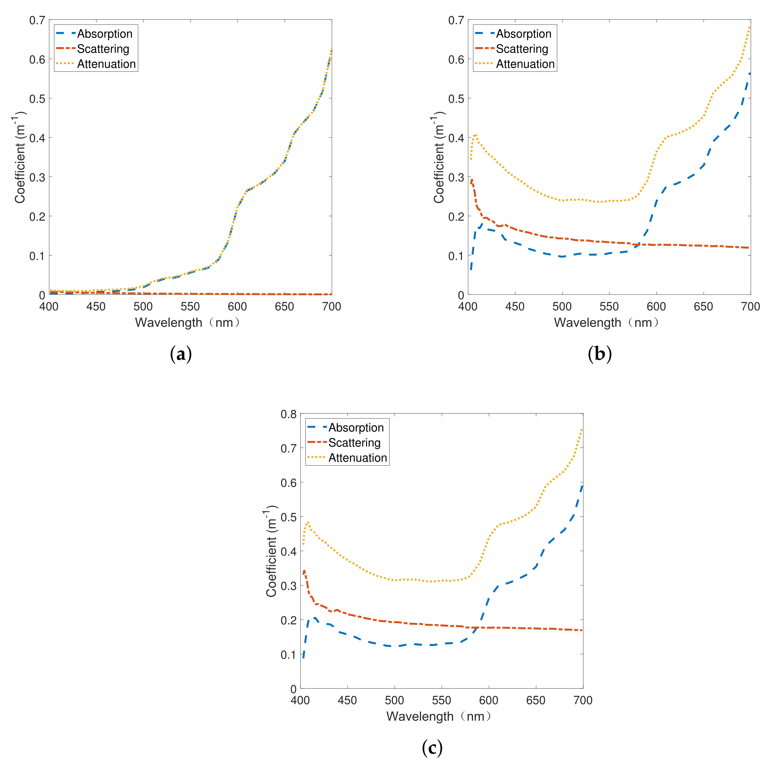
• Underwater laser communication channel modeling and loss analysis: The effects of various substances in the water body on the underwater laser communication channel are analyzed, and the corresponding computational model is established. The optical path loss and the attenuation characteristics of the light source in the underwater channel are calculated.
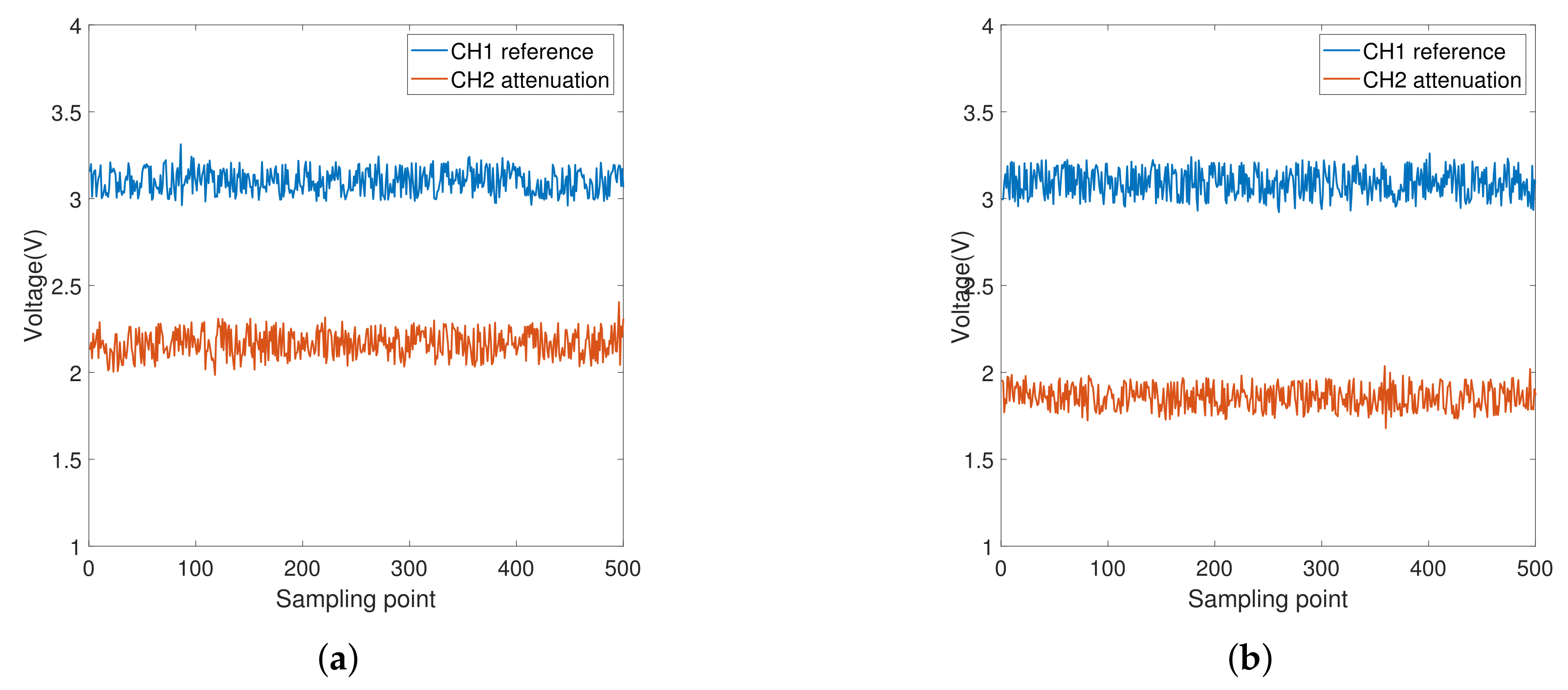
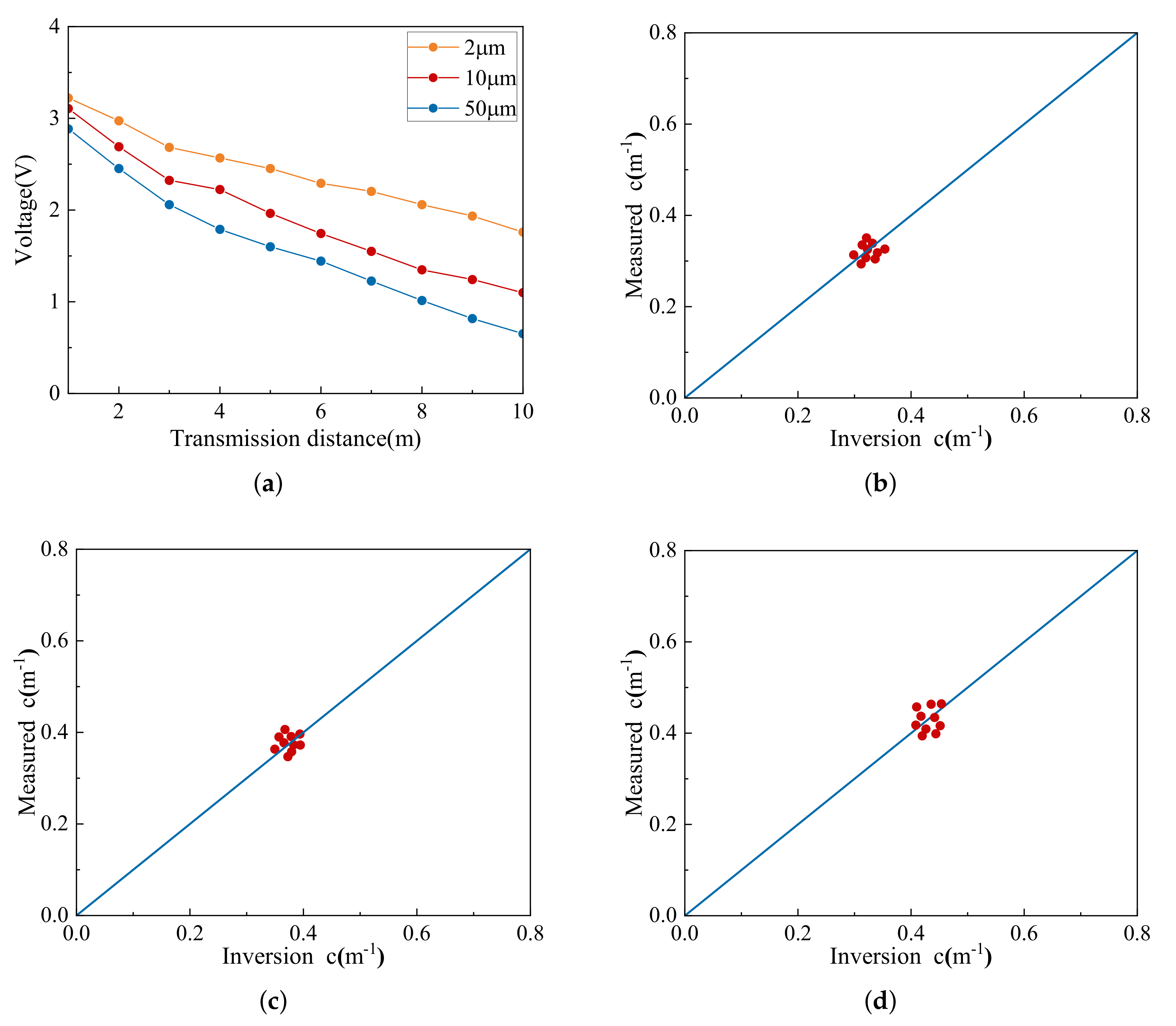
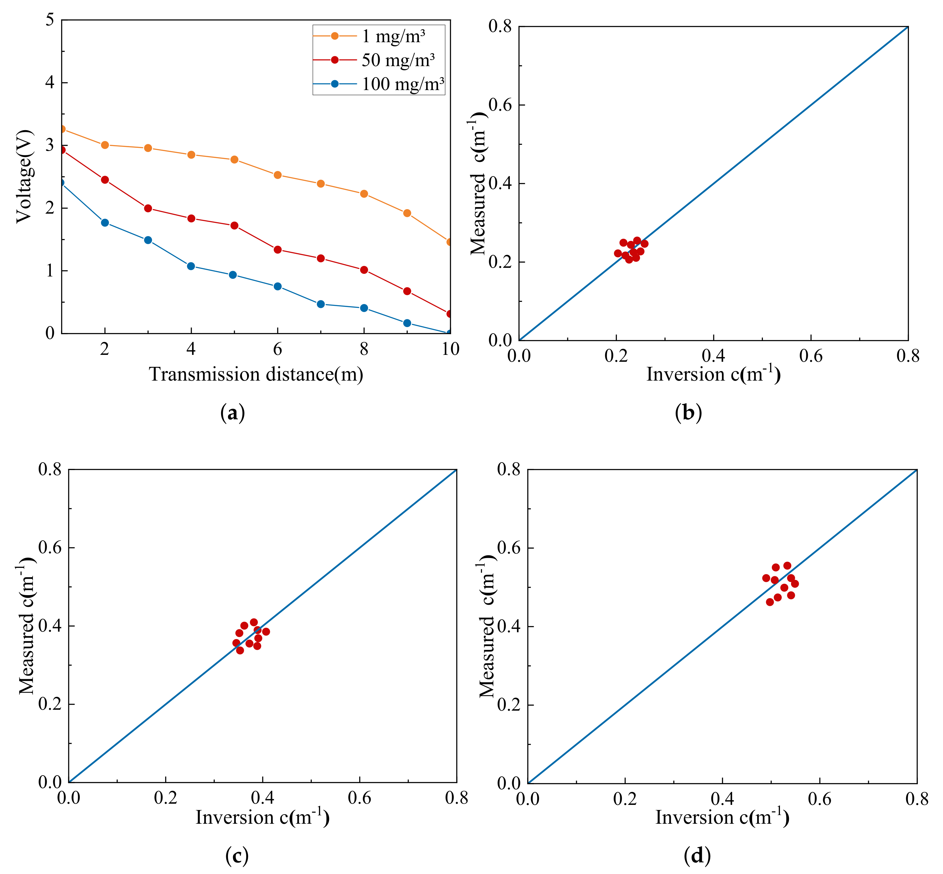
• Field measurement system design and experimental validation: A field measurement system is designed to measure the attenuation of underwater laser channels. The correctness of the computational model in the underwater laser communication channel is verified in different water quality environments. The calculation results are compared with underwater hyperspectral absorption coefficient spectrometer (ACS) measurements to verify the accuracy.
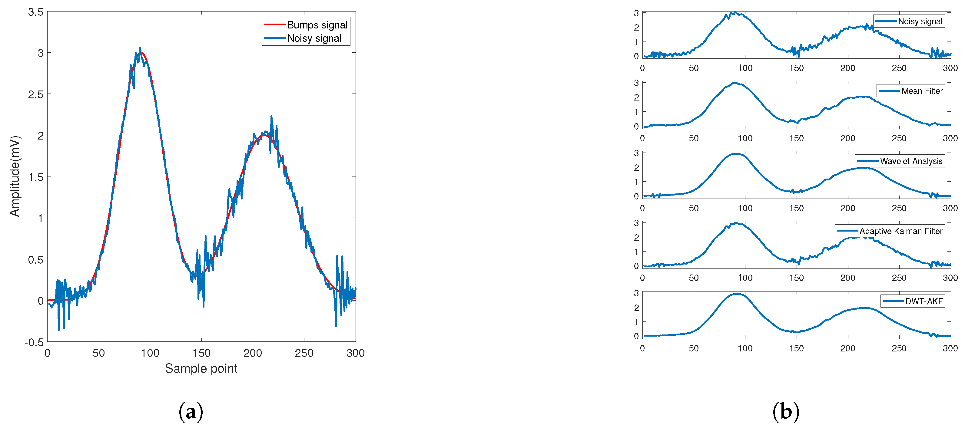
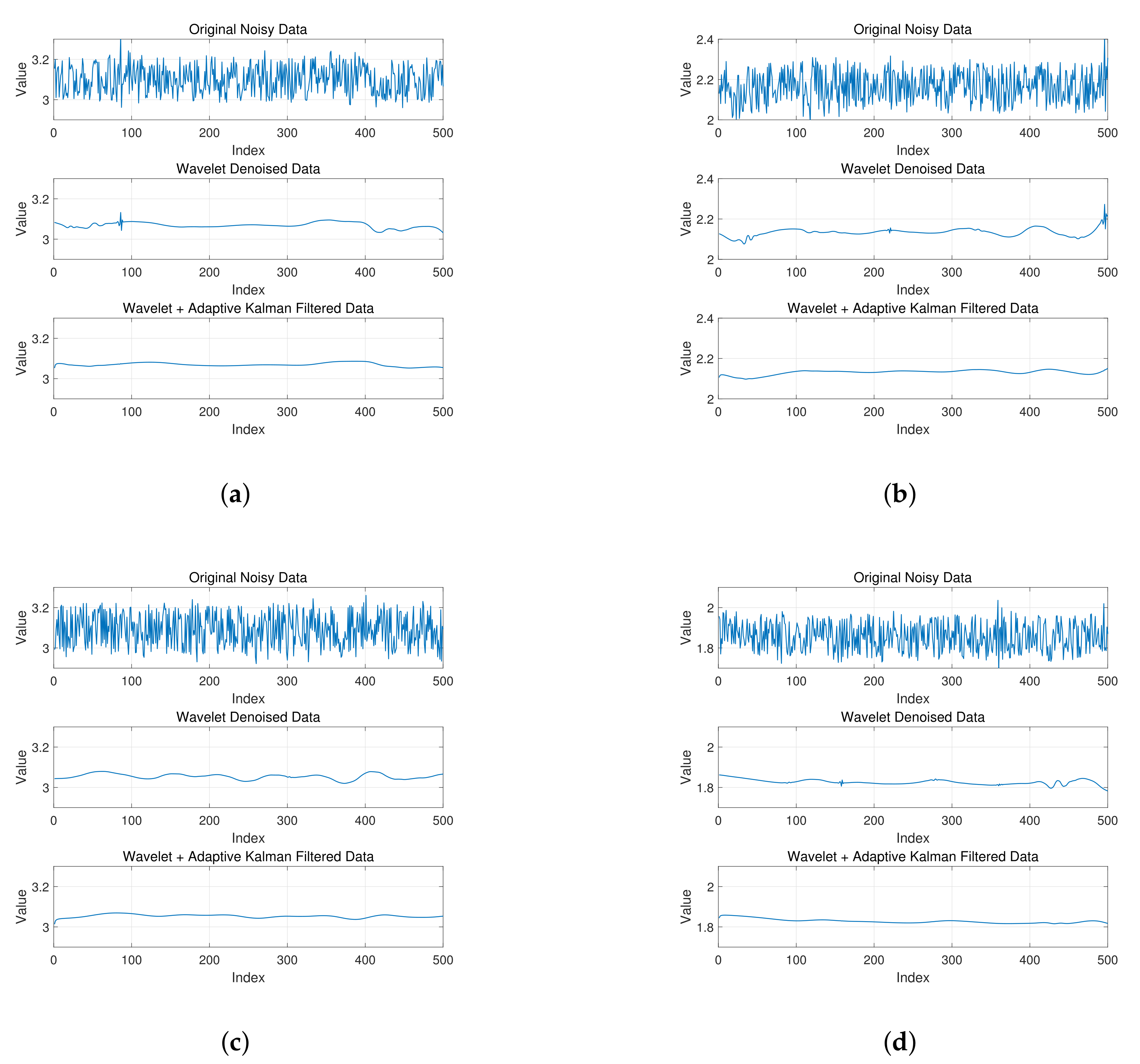
• Fusion filtering algorithms to optimize data quality: A fusion filtering algorithm based on wavelet analysis denoising and adaptive Kalman filtering is proposed to improve the reliability of collected data. Wavelet analysis denoising removes random noise and adaptive Kalman filtering removes systematic noise to enhance signal accuracy.

The remainder of this paper is organized as follows. Section 2 reviews relevant studies on the underwater laser communication channel model. Section 3 details the materials and methods used for the analysis of the attenuation model and the design of the calibration setup. Section 4 presents the experimental results along with data analysis. Finally, Section 5 concludes the study and outlines future work.

2. Related Works

Underwater laser communication has become one of the hot directions of underwater information transmission research in recent years due to its advantages of high rate, low delay, and high confidentiality [12]. Due to the significant absorption and scattering of laser light by seawater medium, the modeling and performance evaluation of the communication channel have become the key issues in this field of research.

The current research on the channel characteristics of underwater laser communication mainly focuses on two directions: one is to establish a physical model based on the theory of radiative transfer, the Beer–Lambert law, and so on, in order to explain the propagation loss of light under different water conditions. The second is to quantitatively analyze the propagation path of photons in seawater, the scattering process, and its effect on the communication performance by means of numerical simulation methods, especially Monte Carlo simulation.

Firstly, the communication channel characteristics in seawater are analyzed by building a physical model. Mooradian et al. [13] constructed an underwater optical transmission channel model under the ideal conditions of assuming that the laser beam is free from external interference and the signal is not distorted during the underwater propagation process, and based on which they derived a mathematical function expression for the propagation of the laser pulse in the time domain. Wei et al. [14] developed an impulse response model based on an inverse Gaussian function for the UWOC system, which performs well in clear water and short-distance transmission conditions, but it is difficult to cover the propagation characteristics in complex or high-turbidity environments. In addition, the study did not compare and analyze the model results with Monte Carlo simulation results or measured data, and the means of validation were relatively limited. Umar et al. [15] investigated the influence of multiple scattering effects in non-line-of-sight underwater optical wireless communication links, compared and analyzed a variety of underwater transmission models based on different scattering phase functions, and gave the temporal dispersion characteristics in coastal and harbor waters, which provided a theoretical basis and modeling foundation for the subsequent quantitative analysis of BER and other performance metrics in underwater communication links. Shin et al. [16] considered the stochastic obstruction of underwater beam propagation by air bubbles, and combined the bubble obstruction model with the gamma-gamma model to derive the distribution of the composite channel model. The analytical form of the average BER and capacity of the UWOC system based on this composite channel model is finally obtained and verified. Zedini et al. [17] proposed to model the UWOC according to a uniform mixed-exponential generalized gamma distribution and derived an exact closed-form probability density function for the end-to-end signal-to-noise ratio, which can effectively analyze turbulence induced by short-range, temperature gradients, and bubbles.

Secondly, numerical simulations are performed in order to study its channel characteristics. Cox et al. [18] proposed a two-exponential power loss model to analyze the optical transmission performance under different parameter conditions, while the temporal bandwidth under different communication links is analyzed using the phase function of seawater scattering obtained from experimental measurements by Petzold. Based on the underwater laser communication system, Yingluo et al. [19] constructed the channel model and used the MC numerical simulation method to analyze the influence of system parameters on the laser signal transmission performance. Yuan et al. [20] introduced different sampling methods to improve the convergence of the Monte Carlo integration model. Among them, the Monte Carlo integration model based on partially significant sampling has higher computational efficiency in high-order scattering scenarios. Sahu et al. [21] used Monte Carlo numerical simulations to study the effect of pulse compression caused by particle scattering on the attenuation probability. Furthermore, they derive an analytical expression for focal length and minimum pulse length, which is a function of channel characteristics, incident pulse length, and initial value. In recent years, some studies have begun to focus on the modeling of underwater optical communication channels in environments with spatial variations or non-uniform conditions. Ramley et al. [22] used Monte Carlo simulation methods to model the propagation characteristics of photons in seawater, proposing mathematical models suitable for single-pulse and multi-pulse propagation in both uniform and non-uniform media under different water conditions. Building on this work, the team further developed a photon tracking model based on discrete equations, combining Monte Carlo methods to assess the impact of different scattering mechanisms on the distribution of received photons. This enabled a quantitative analysis of optimal design parameters for underwater communication links under varying field-of-view angles and water body types [23].

3. Materials and Methods

3.1. Modeling of Underwater Laser Transmission

The total attenuation of the underwater laser communication channel is mainly composed of geometric attenuation and seawater attenuation. The former reflects the reduction of energy density due to beam expansion in the process of laser propagation in space, while the latter mainly originates from the absorption and scattering effect of seawater on the laser signal, which together determine the attenuation characteristics of the signal in the transmission process.

Geometric attenuation refers to the loss of signal energy during underwater transmission of a laser signal due to the continuous expansion of the beam and the fact that some of the optical energy is beyond the receiving range of the receiver. Figure 2 shows the geometric expansion of light in the transmission process, d is the distance between the underwater laser signal receiver and transmitter, $\theta$ is the divergence angle of beam at the transmitter, and r is the radius of the spot after beam expansion.

The energy loss incurred during the propagation of light through water when a laser beam is emitted from a transmitter in different directions has been investigated through numerical simulations [24]. The optical transmission power after beam expansion is uniformly distributed over the field of view, and the received power is the same at each point in the field of view. So, the power after beam expansion can be expressed by the ratio of the effective received area to the spot area. When the incident wavelength is large enough, the additional focal dispersion effects since light passing through the lens increases the energy loss [25].

Facing long-range underwater wireless optical communication, the transmission loss is closely related to transmission distance, the light-sensitive area at the receiver, and the divergence angle of the light source at the transmitter [26]. The transmitter of the light source will produce some losses when it emits light, i.e., the luminous efficiency ${\eta }_i$. The spatial loss caused by factors such as the size and spatial position of the receiver, and the angle of the receiving plane, is called receiving efficiency ${\eta }_r$. The laser transmission process is affected by random noise generated by factors such as temperature and spatial illumination, which is unique and random. According to the above influencing factors, the received power of the underwater laser can be obtained as follows:

$$P_r=P_i\times {\eta }_i\times {\eta }_r\times \eta \times \left[{\displaystyle \frac{a_r^2}{{(\Delta dtan\theta +a_i)}^2}}\right]\times e^{(-c(\lambda )\times \Delta d)}$$

(1)

where $P_i$ is the transmitted optical power, $P_r$ is the received optical power, $a_i$ is the radius of the optical transmission aperture, $a_r$ is the radius of the optical receiver aperture, $c\left(\lambda \right)$ is the total attenuation coefficient of seawater, and $\eta$ denotes the influence of other additional effects.

Seawater contains a large number of soluble substances and suspended particles, the type and concentration of which have significant variations in time and space, and these components have an important influence on the optical properties of seawater and show a strong spatial and temporal correlation. The attenuation of a light beam in seawater is mainly determined by its inherent optical properties, including absorption and scattering. Among them, absorption refers to the fact that part of the energy of incident light is converted into other forms such as thermal energy and chemical potential energy by water molecules, dissolved substances, or particles in seawater in the process of propagation, which leads to the actual energy loss of the underwater light field. The scattering effect refers to the light in the interaction with various particles in the water body under the propagation direction change, although it does not cause energy loss, but will lead to the redistribution of light energy in space, thus affecting the direction and uniformity of the underwater light field.

Figure 3 shows the geometrical model of seawater’s intrinsic optical properties with a thickness of $△d$ and $△V$ [27]. When incident light with transmission power $P_i\left(\lambda \right)$ and wavelength $\lambda$ irradiates seawater, the absorption of seawater causes power attenuation $P_a\left(\lambda \right)$, the scattering of seawater causes power attenuation $P_b\left(\lambda \right)$, and the unaffected optical power $P_t\left(\lambda \right)$. From the point of view of energy conservation, this process can be expressed as

$$P_i\left(\lambda \right)=P_a\left(\lambda \right)+P_b\left(\lambda \right)+P_t\left(\lambda \right)$$

(2)

Due to the complexity of the interaction process between light and matter, and the different effects of various physical fields on optical properties, these lead to the attenuation of light energy by water. According to the light absorption characteristics of pure seawater, suspended particles, dissolved organic matter, plankton, and other substances, the total absorption coefficient of seawater can be expressed as [28]:

$$a\left(\lambda \right)=a_w\left(\lambda \right)+a_y\left(\lambda \right)+a_c\left(\lambda \right)+a_x\left(\lambda \right)$$

(3)

where $a_w\left(\lambda \right)$ denotes the absorption coefficient of pure seawater, $a_y\left(\lambda \right)$ denotes the absorption coefficient of dissolved organic matter, $a_c\left(\lambda \right)$ denotes the absorption coefficient of plankton, $a_x\left(\lambda \right)$ denotes the absorption coefficient of suspended particles, and their units are ${\mathrm{m}}^{-1}$.

The light scattering of seawater mainly comes from the water body itself, chlorophyll, and suspended particles. In addition, the changes in pressure and temperature affect the scattering coefficient of pure seawater. The total scattering coefficient of seawater can be expressed as

$$b\left(\lambda \right)=b_w\left(\lambda \right)+b_c\left(\lambda \right)+b_x\left(\lambda \right)$$

(4)

where $b_w\left(\lambda \right)$ denotes the scattering coefficient of pure seawater, $b_c\left(\lambda \right)$ denotes the scattering coefficient of plankton, $b_x\left(\lambda \right)$ denotes the scattering coefficient of suspended particles, and their units are ${\mathrm{m}}^{-1}$.

In conclusion, the total underwater laser attenuation coefficient includes seawater absorption and seawater scattering [29,30,31], which can be expressed as

$$\begin{array}{cc}\hfill c\left(\lambda \right)& =a\left(\lambda \right)+b\left(\lambda \right)\hfill \\ \hfill & =a_w\left(\lambda \right)+0.243e^{(-0.014\times (\lambda -440\left)\right)}+0.025\times C+0.198e^{(-0.01\times (\lambda -440\left)\right)}\hfill \\ \hfill & +b_w\left(\lambda \right)+(550/\lambda )0.30C^{0.62}+1.151{(400/\lambda )}^{1.7}+0.341074{(400/\lambda )}^{0.3}\hfill \end{array}$$

(5)

where C is the chlorophyll concentration.

The attenuation coefficient curve of chlorophyll concentration with wavelength is shown in Figure 4. It is not difficult to find that, as the chlorophyll concentration increases, the total attenuation coefficient of seawater increases. In addition, as the wavelength changes, the chlorophyll concentration and total attenuation coefficient of seawater show a certain trend.

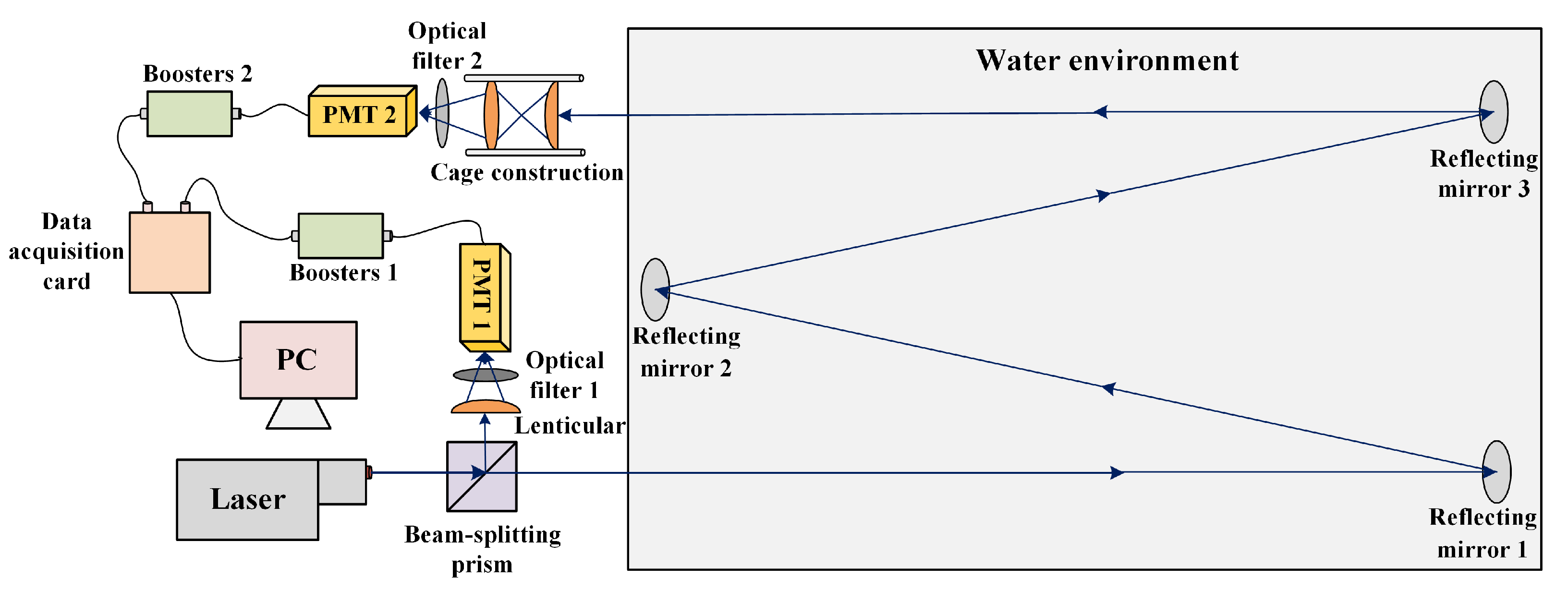
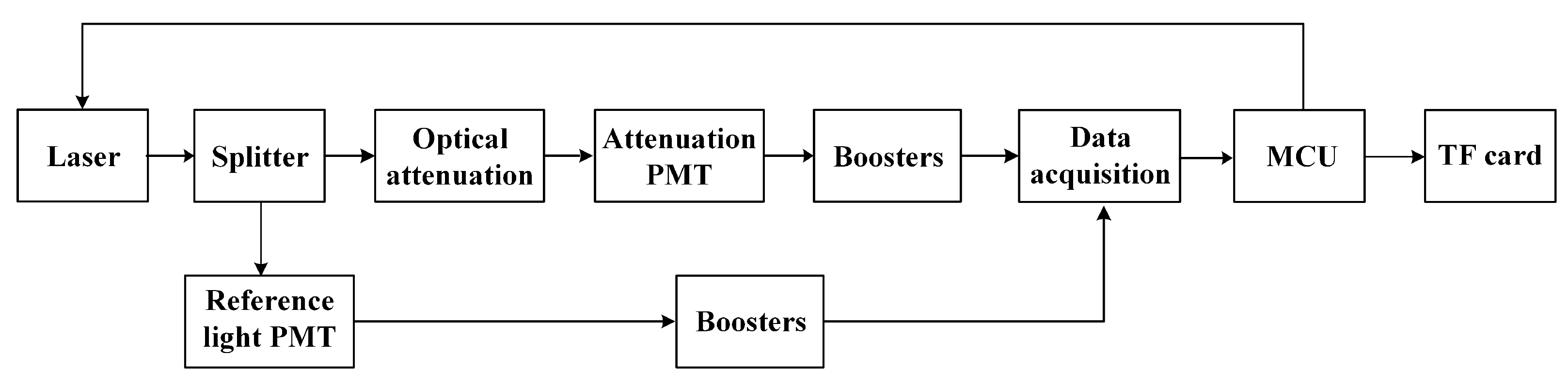
3.2. Underwater Laser Channel Attenuation Measurement System

3.2.1. System Design and Construction

In order to study the propagation characteristics of a laser in a seawater environment and accurately obtain its attenuation law under different water conditions, this paper designs and builds a system of underwater laser channel attenuation measurements. The system can simulate the laser transmission process under real seawater conditions in a controlled experimental environment, and realize high-precision and quantitative measurements of the attenuation generated by laser energy propagation in the water body. The system measures the initial intensity of the laser and the received intensity after passing through the water body by constructing two optical paths, the reference channel and the main channel, so as to eliminate the error caused by the fluctuation of the power of the laser itself and accurately reflect the real attenuation effect of the water body on the optical signal. The overall structure of the system is shown in Figure 5, which mainly includes the laser transmitter module, the reference channel, the main underwater channel, the optical receiver module, and the signal amplification and data acquisition module. Some main parameters of these devices in this paper are shown in

Table 1. Parameters of this paper.

Parameters	${\mathit{\eta }}_{\mathit{i}}$	${\mathit{\eta }}_{\mathit{r}}$	${\mathit{a}}_{\mathit{i}}$	${\mathit{a}}_{\mathit{r}}$	$\mathit{\theta }$	$\mathit{\gamma }$
Value	0.97	0.91	3 mm	8 mm	1.12 mrad	$1.5\times {10}^5$ A/W

.

The core light source of the system is a DPS-532-A Nd:YAG laser produced by Changchun New Industry, with an output wavelength of 532 nm and good monochromaticity and directivity, which can meet the demand for stable transmission in highly scattering water bodies. The collimated beam from the laser first passes through a beam-splitter prism with a beam split ratio of 1:9 for initial optical path division. The prism splits the laser beam stably into two mutually perpendicular beams, of which 10% of the luminous flux is reflected by the beam splitter to form a reference optical channel, which is used for real-time monitoring of the initial emitted intensity of the laser source, while the remaining 90% of the luminous flux enters the main optical channel in the form of transmission, which is used for subsequent attenuation measurements after propagation through the underwater channel.

After beam splitting, the reference beam is first focused uniaxially and linearly through a cylindrical lens to improve the spatial beam distribution and increase reception efficiency and detection sensitivity. Subsequently, the beam is passed through a neutral density filter with a transmittance of 50%, which is used to attenuate the light intensity appropriately so that too high a luminous flux does not lead to a nonlinear response of the subsequent detectors or to a saturated operating region. The optically shaped reference signal is detected by a high-sensitivity Japan Hamamatsu H10721-210 photomultiplier tube 1 (PMT1), which is capable of converting weak optical signals into electrical signals with a good linear response, providing the system with high signal-to-noise reference data. The reference channel is set up to record the initial emission intensity of the laser source and serve as a benchmark for system calibration, effectively eliminating the effects of laser power fluctuations and electrical interference on the measurement results.

The main beam is separated by a beam-splitter prism and enters the experimental tank, constituting an underwater laser propagation channel. In order to simulate a longer underwater light path and enhance the sensitivity of the system, the system arranges multiple mirrors in the water tank to construct a propagation path with multiple reflections. Each reflection is accompanied by a certain length of water propagation, effectively simulating the gradual attenuation of the laser in the water. This design not only improves the ability to distinguish the weak attenuation, but also facilitates the flexible control of the total propagation distance. Finally, the laser light after multiple reflections is output from the end of the water tank and enters the receiver module.

In the optical receiver module, the laser signal propagated and attenuated by the underwater channel is first focused by the cage structure optical system composed of plano-convex lenses and biconvex lenses. The optical structure has good axial collimation and focusing ability, which can effectively improve the spatial coupling efficiency of the incident light, thus enhancing the stability and signal-to-noise ratio of the received signal. The focused beam is then passed through a neutral density filter with a transmittance of 10%, which is used to further suppress excessive light intensity and avoid a nonlinear response or saturation distortion of the detector due to excessive incident power. Ultimately, the modulated optical signal is received by a high-sensitivity Japan Hamamatsu H10721-210 photomultiplier tube 2 (PMT2), which enables high-precision detection of the laser signal attenuated by the water in the main channel.

In order to improve the overall signal-to-noise ratio of the system, the two PMT channels are equipped with Japan Hamamatsu C9999 low-noise amplifiers and C10709-C4 regulated power supplies for amplifying and stabilizing the power supply of weak photoelectric signals. The amplified analog signals are transmitted to the control computer via a Handyscope HS5 high-speed data acquisition card, and the upper computer software collects, displays, and records the signal strength data in real time.

The circuit design of the underwater laser channel attenuation measurement system is shown in Figure 6. The core of the system is coordinated and controlled by a microcontroller unit (MCU), which is responsible for laser emission triggering, data processing, and storage control. The laser emits a blue-green laser under the control of the MCU, which passes through a beam splitter for spectral processing. The splitter divides the laser into two paths, and one path is used as the reference light, which is directly received by the reference light PMT through the reference light channel, and the signal is used for subsequent data comparison and channel correction. The other part of the laser beam is used as a working beam and enters directly into the underwater laser transmission channel, where the laser propagates in the water column and undergoes attenuation. The attenuated laser signal is focused through the receiving lens and received by the attenuating PMT, which converts the incident optical signal into the corresponding electrical signal with high sensitivity, and since the output signal is usually weak, it needs to be amplified by the amplifier module, and the amplified signal is transmitted to the data acquisition module.

The data acquisition module simultaneously receives the amplified digital signals of the reference light PMT and the attenuated PMT and sends them to the MCU for further analysis. The MCU calculates the light intensity attenuation coefficients of the underwater laser transmission channel based on the intensity difference between the reference light and the attenuated light. Finally, the MCU writes all the processed experimental data into a TF card, which facilitates subsequent offline processing, analysis, and result verification.

The desktop measurement device built in the laboratory is shown in Figure 7; Figure 7a shows the measured underwater laser communication channel in a water tank of $1\mathrm{m}\times 0.6\mathrm{m}\times 0.4\mathrm{m}$; Figure 7b shows the detailed optical design. The continuous measuring scene is illustrated in Figure 7c; the working frequency is 1 Hz. The physical diagram of the system construction is shown in Figure 7d.

3.2.2. Calculation of Optical Characterization Parameters of Water Bodies

To improve the accuracy of seawater column attenuation measurement, this paper introduces the following parameters: transmittance of dichroic prism is ${\zeta }_1$, transmittance of filter 1 is ${\zeta }_2$, transmittance of filter 2 is ${\zeta }_3$, optical path device loss is ${\zeta }_4$, and photoelectric conversion coefficient of PMT is $\gamma$.

Let the reference optical PMT output current be $I_a$. The reference optical path power can be expressed as

$$P_1={\displaystyle \frac{I_a}{{\zeta }_1{\zeta }_{2}R\gamma }}$$

(6)

where R is the responsiveness of the PMT.

Let the measured PMT output current be $I_b$. The measured attenuation optical path can be expressed as

$$P_2={\displaystyle \frac{I_b}{{\zeta }_3{\zeta }_{4}R\gamma }}$$

(7)

The attenuation coefficient of a seawater sample for laser light can be calculated as

$$c={\displaystyle \frac{1}{d}}ln{\displaystyle \frac{P_1{\eta }_i{\eta }_r\eta \left[\frac{a_r^2}{{(dtan\theta +a_i)}^2}\right]}{P_2}}$$

(8)

3.3. Post-Processing Denoising Algorithm

3.3.1. Data Correction and Calibration

• Reference light calibration
  In order to eliminate the effects of laser output power fluctuations or changes in laser source intensity on the measured results, in each measurement, the reference light intensity is measured through a reference optical path, and the measured signal is used to normalize with the reference signal.

  $$I_{corrected}={\displaystyle \frac{I_{measured}}{I_{reference}}}$$

  (9)

  where $I_{corrected}$ is the corrected signal, $I_{measured}$ is the measured signal, and $I_{reference}$ is the reference signal.
• Dark current calibration
  Photodetectors still generate a weak current (dark current) when there is no input light signal, which can interfere with the actual light signal.

  $$I_{net}=I_{measured}-I_{dark}$$

  (10)

  where $I_{dark}$ is the dark current signal, $I_{measured}$ is the actual measured signal, and $I_{net}$ is the corrected signal.
• Ultrapure water calibration
  Ultrapure water is applied to set the calibration coefficients of attenuation coefficients, which can improve the accuracy and reliability of the measurement system.

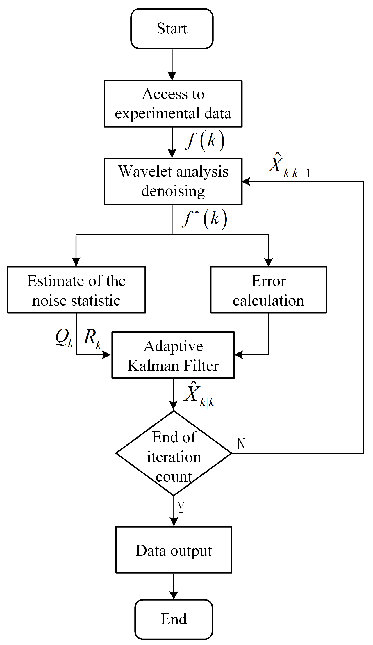
3.3.2. Multi-Scale Dynamic Denoising Method Based on DWT-AKF

During the detection process of our designed device, the collected signal value contains noisy light signals due to the influence of environmental background noise, the internal noise of the device, and external interference.

The collected signal of the proposed device can be expressed as [32]

$$d\left(k\right)=f\left(k\right)+\epsilon \times z\left(k\right),k=1,\cdots ,n$$

(11)

where $d\left(k\right)$ denotes the noise-containing signal, $f\left(k\right)$ denotes the sampled signal without noise, $z\left(k\right)$ denotes the independent and identically distributed Gaussian white noise $N(0,1)$, $\epsilon$ denotes the noise level, and n denotes the signal length.

Considering that the observed signal is a series of measurement data with noise, this paper firstly performs a multi-scale wavelet transform, utilizing the superiority of the wavelet transform in time–frequency analysis, decomposes different scale features of the signal, and extracts approximation coefficients and detail coefficients. The statistical properties of the noise are estimated by analyzing the detail coefficients, and the observation noise covariance is adjusted adaptively. Then, the low-frequency components of the main signal are preserved by wavelet reconstruction to obtain the preliminary denoised signal. The denoised signal is used as the measured value input for adaptive Kalman filtering, and the system state and noise covariance are updated at each moment, so that the filter realizes the optimal estimation of the data while reducing the noise, thus improving the accuracy and stability of the signal; the program flowchart for DWT-AKF denoising is shown in Figure 8.

The wavelet analysis denoising process can be divided into three steps:

• The wavelet decomposition of collected data
  This process can be expressed as

  $$W_{0}s=W_{0}f+W_{0}z$$

  (12)

  where s denotes the collected data signal vector $s\left(1\right)$, $s\left(2\right)$, ⋯, $s\left(n\right)$, f is the real signal vector, and z is the Gaussian random vector.
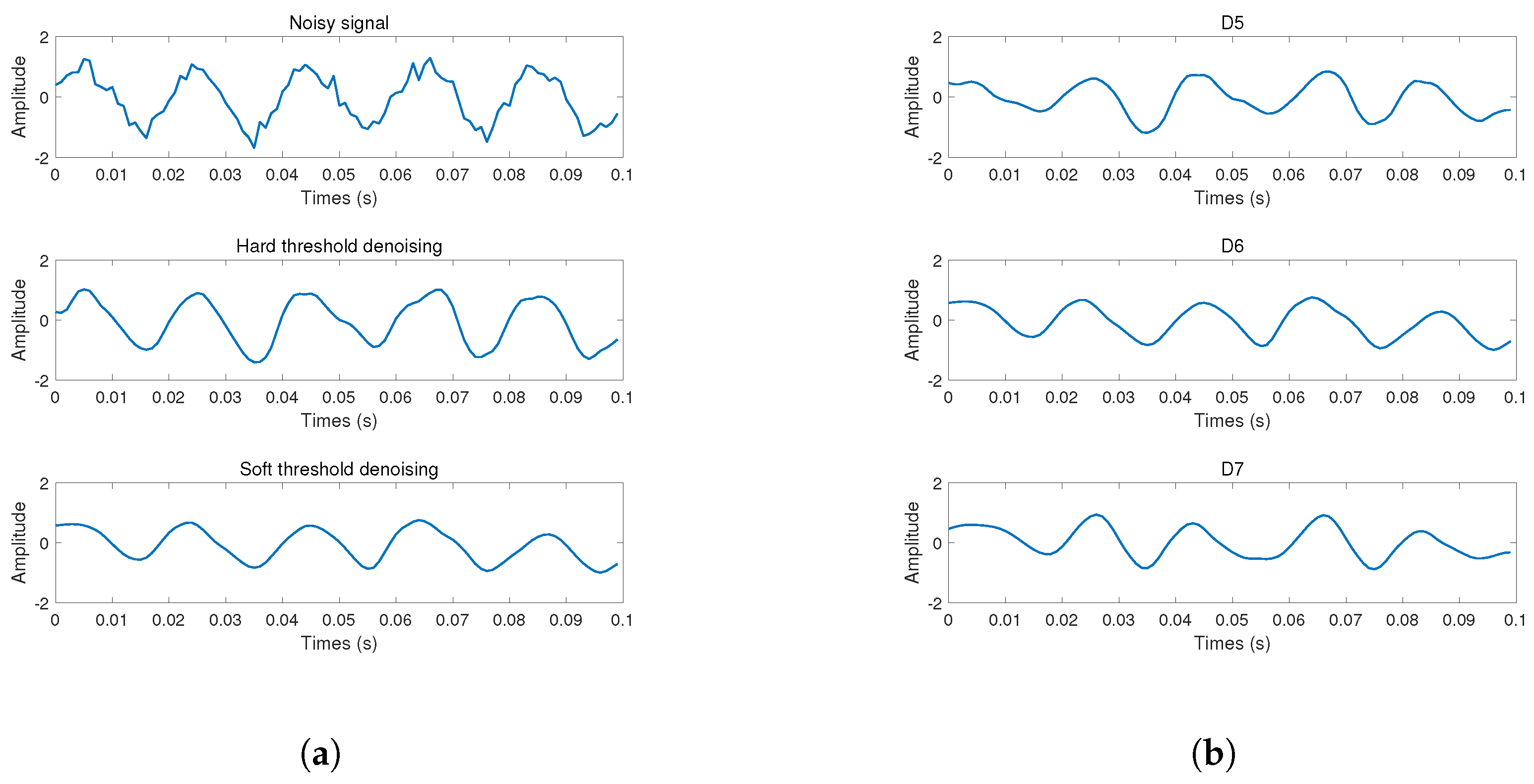
• The threshold operation of the wavelet coefficient $W_0$
  The threshold functions include hard threshold functions and soft threshold functions. When the signal is processed by the hard threshold function, the signal is prone to oscillation. The soft threshold function can smooth the signal [33]. Hence, this paper uses the soft threshold function for threshold operation. Among them, the soft threshold expression [34] is

  $${\widehat{\omega }}_{i,j}=\left\{\begin{array}{cc}sgn\left({\omega }_{j,k}\right)\left(\right|{\omega }_{j,k}|-{\lambda }_N),\hfill & |{\omega }_{j,k}|\ge {\lambda }_N\hfill \\ 0,\hfill & |{\omega }_{j,k}|<{\lambda }_N\hfill \end{array}\right.$$

  (13)

  where

  $$sgn\left(x\right)=\left\{\begin{array}{cc}+1,\hfill & x\ge 0\hfill \\ -1,\hfill & x<0\hfill \end{array}\right.$$

  (14)

  In addition, the selection of ${\lambda }_N$ is

  $${\lambda }_N=\sigma \sqrt{2logn}$$

  (15)

  Further, the estimated noise level is defined as

  $$\sigma ={\displaystyle \frac{\mathrm{median}\left(\left|{\omega }_{j,k}\right|\right)}{0.6745}}$$

  (16)

  where $\mathrm{median}($) denotes the operation of taking the middle value; ${\omega }_{j,k}$ and ${\widehat{\omega }}_{i,j}$ are the wavelet coefficients before and after the denoising process, respectively.
• The signal reconstruction based on wavelet coefficients
  An inverse transformation $W_0^{-1}$ is applied to the processed wavelet coefficients to reconstruct the signal, which can be expressed as

  $$f^{*}=W_0^{-1}{\eta }_{\lambda }{W}_{0}s$$

  (17)

  where $f^{*}$ is the acquired signal after denoising and ${\eta }_{\lambda }{W}_{0}s$ denotes the wavelet coefficients after the thresholding operation.

Wavelet decomposition thresholding denoising is used to enhance the recognition of signals that are easily confused with noise, and Kalman filtering plays the role of optimal estimation, smoothing the data and removing singular values, thus compensating for the shortcomings of wavelet analysis. The classical Kalman filtering algorithm is prone to the divergence phenomenon, resulting in unreliable state estimation. In order to overcome the dispersion phenomenon, an adaptive Kalman filtering algorithm is used.

In the wavelet analysis denoising of data processing, this paper uses a multiple-scale wavelet transform and soft threshold function to denoise the signal received by the PMT element and reconstruct the signal from the inverse wavelet transform. Then, this paper uses the reconstructed signal as the input value of the adaptive Kalman filter.

The state equation and observation equation of this system are expressed as

$$X_k=A_k{X}_{k-1}+B_k{U}_k+{\omega }_k$$

(18)

$$Z_k=H_k{X}_k+{\upsilon }_k$$

(19)

where $X_k$, $Z_k$, and $U_k$ denote system state, measurements, and system controller at moment k, respectively. $A_k$ is the system state transfer matrix, $B_k$ is the control input matrix and $B_k=0$, and $H_k$ is the observation matrix. ${\omega }_k$ and ${\upsilon }_k$ are the process noise and measurement noise of this system, respectively. $Q_k$ and $R_k$ are the covariance matrices.

The traditional Kalman filtering process [35] consists of two phases: the prediction phase and the correction phase.

• Prediction phase
  The prediction equation of the system state can be expressed as

  $${\widehat{X}}_{k|k-1}=A_{k|k-1}{\widehat{X}}_{k-1|k-1}+B_{k|k-1}{U}_k$$

  (20)

  where ${\widehat{X}}_{k|k-1}$ is the predicted value at moment $k-1$ for moment k, and ${\widehat{X}}_{k-1|k-1}$ is the optimal estimation of the previous state.
  In addition, the covariance prediction equation of this state can be calculated as

  $$P_{k|k-1}=A_{k|k-1}{P}_{k-1|k-1}{A}_{k|k-1}^{\mathrm{T}}+Q_k$$

  (21)

  where $P_{k|k-1}$ denotes the prediction of systematic error covariance at moment $k-1$ for moment k, $P_{k-1|k-1}$ denotes the estimate of covariance matrix corresponding to ${\widehat{X}}_{k-1|k-1}$, $A_{k|k-1}^{\mathrm{T}}$ denotes the transpose matrix of $A_{k|k-1}$, and $Q_k$ denotes the covariance matrix of the systematic process ${\omega }_k$.
  The system state transfer matrix $A_k$ and the observation matrix $H_k$ are initialized as, respectively,

  $$A_0=\left[\begin{array}{cccc}1\hfill & 1\hfill & 0\hfill & 0\hfill \\ 0\hfill & 1\hfill & 0\hfill & 0\hfill \\ 0\hfill & 0\hfill & 1\hfill & 1\hfill \\ 0\hfill & 0\hfill & 0\hfill & 1\hfill \end{array}\right]$$

  (22)

  $$H_0=\left[\begin{array}{cccc}1\hfill & 0\hfill & 0\hfill & 0\hfill \\ 0\hfill & 0\hfill & 1\hfill & 0\hfill \end{array}\right]$$

  (23)
• Calibration phase
  The estimation equation of the system filter can be expressed as

  $${\widehat{X}}_{k|k}={\widehat{X}}_{k|k-1}+K{g}_k(Z_k-H_k{\widehat{X}}_{k|k-1})$$

  (24)

  where ${\widehat{X}}_{k|k}$ denotes the optimal estimate at moment k; $Z_k$ denotes the reconstructed signal value after wavelet analysis inverse transformation.
  In addition, the gain equation of the Kalman filter can be calculated as

  $$K{g}_k={\displaystyle \frac{P_{k|k-1}{H}_k^{\mathrm{T}}}{H_k{P}_{k|k-1}{H}_k^{\mathrm{T}}+R_k}}$$

  (25)

  where $H_k^{\mathrm{T}}$ denotes the transpose matrix of $H_k$; $R_k$ denotes the covariance matrix of system process ${\upsilon }_k$.
  Therefore, the updated error covariance matrix can be expressed as

  $$P_{k|k}=(I-K{g}_k{H}_k)P_{k|k-1}$$

  (26)

  where I is the unit matrix.

In the classical Kalman filtering algorithm, both ${\omega }_k$ and ${\upsilon }_k$ are regarded as ideal zero-mean Gaussian white noise, and covariance arrays $Q_k$ and $R_k$ are known [36]. To avoid the divergence phenomenon, an adaptive Kalman filtering algorithm is used.

According to the standard Kalman filter, the error $e_k$ between the measured value and the estimated value can be obtained as

$$e_k=Z_k-H_k{\widehat{X}}_{k|k-1}$$

(27)

In addition, the covariance of $e_k$ is

$$C_{zk}=E\left(e_k{e}_k^{\mathrm{T}}\right)=H_k{P}_{k|k-1}{H}_k^{\mathrm{T}}+R_k$$

(28)

The most approximate estimate ${\widehat{C}}_{zk}$ of $C_{zk}$ can be obtained from a new interest sequence $\left\{e_k\right\}$ with signal interval length n.

$${\widehat{C}}_{zk}={\displaystyle \frac{1}{n}}\sum _{i=0}^{n-1}{e}_{k-i}{e}_{k-i}^{\mathrm{T}}$$

(29)

As a result, the measurement noise covariance estimation equation $R_k$ can be expressed as

$${\widehat{R}}_k={\widehat{C}}_{zk}-H_k{P}_{k|k-1}{H}_k^{\mathrm{T}}$$

(30)

Then, the noise covariance estimation equation $Q_k$ of this system can be expressed as

$${\widehat{Q}}_k=K{g}_k{\widehat{C}}_{zk}K{g}_k^{\mathrm{T}}$$

(31)

The adaptive Kalman filter processes the observation data and makes appropriate corrections to the parameters of the unknown system model and the statistical characteristics of noise, which weakens the impact of model errors and makes the filtering results closer to the true value.

3.4. Validation of Attenuation Measurements

In order to verify the inversion ability of the constructed laser transmission model on the attenuation coefficient under different seawater conditions, the ACS is used as the reference measurement equipment in this paper, as shown in Figure 9. The instrument is based on the principle of high-precision dual-channel spectroscopic measurement, which can synchronously obtain the absorption coefficient $a\left(\lambda \right)$ and attenuation coefficient $c\left(\lambda \right)$ of seawater in the band of 400–750 nm. ACS adopts a dual-optical-range structure design, which can measure the absorption and attenuation channels independently, and significantly reduce the systematic error in the non-ideal optical conditions through the internal optical-range correction and scattering compensation. The system errors are measured under non-ideal optical conditions. With its good spectral resolution and measurement stability, ACS has become a standardized measurement tool widely used in marine optics research.

To quantitatively evaluate the ability of the constructed laser transmission model to invert the attenuation coefficient under different seawater conditions, this paper selects the statistical index correlation coefficient $R^2$ to compare and analyze the consistency between the model inversion values and the measured values of ACS.

$$R^2=1-{\displaystyle \frac{{\displaystyle \sum _{i=1}^m}{(log{f}_i-log{y}_i)}^2}{{\displaystyle \sum _{i=1}^m}{(log\overline{y}-log{y}_i)}^2}}$$

(32)

where m denotes the number of data points, $f_i$ denotes the model inversion value, $y_i$ denotes the ACS measured value, and $\overline{y}$ is the mean value of $y_i$.

$$\overline{y}={\displaystyle \frac{1}{m}}\sum _{i=1}^m{y}_i$$

(33)

4. Experiment and Results

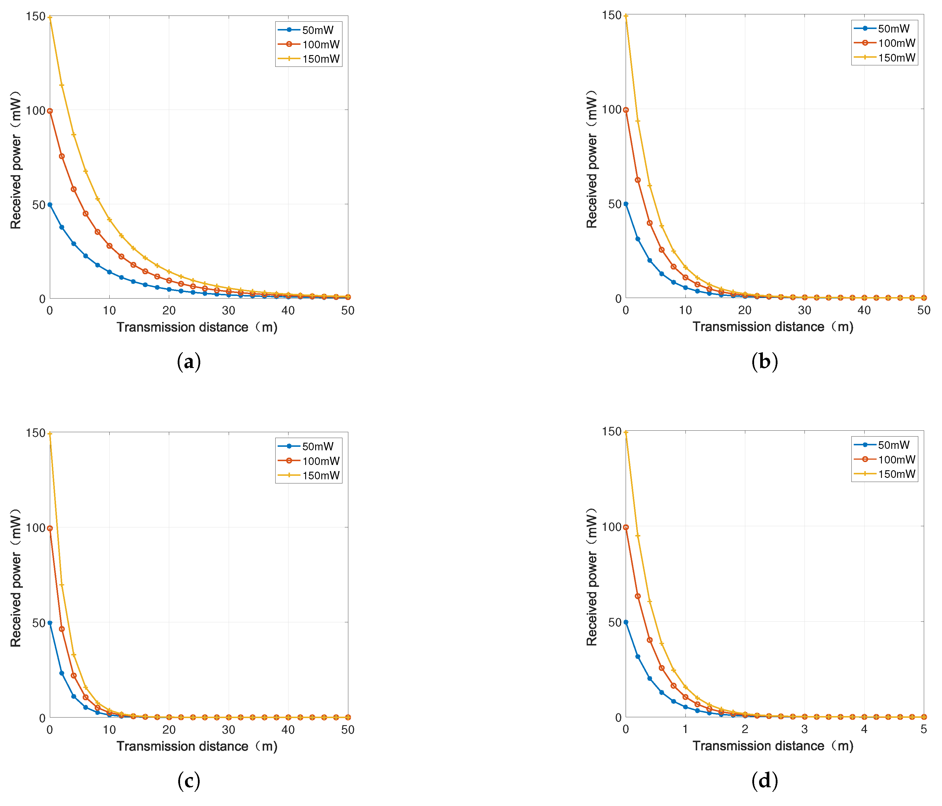
4.1. Underwater Laser Transmission Model Simulation and Analysis

The optical parameters of the four main types of seawater are shown in

Table 2. Optical parameters of four typical types of seawater.

Type of Seawater	a ($\mathit{\lambda }$)	b ($\mathit{\lambda }$)	c ($\mathit{\lambda }$)
Pure seawater	0.053	0.003	0.056
Clear seawater	0.114	0.037	0.151
Coastal seawater	0.179	0.219	0.298
Turbid harbor water	0.295	1.875	2.17

. In the environment of pure seawater, due to its smaller scattering rate, the variation of the beam angle can be effectively reduced, thus ensuring the stability of the beam. In clear seawater, due to its higher concentration of dissolved particles, it has a greater effect on its scattering. In coastal seawater, substances such as plankton, debris, and minerals are the main factors for absorption and scattering. When seawater is disturbed, it produces complex changes that affect the laser transmission process. When turbid harbor water contains a large amount of dissolved and suspended substances, these substances change the nature of the water, thus affecting the efficiency and stability of laser transmission.

The relationship between the power at the receiving end and the transmission distance under different water environments is shown in Figure 10. Within a certain propagation distance, the optical power measured at the receiving end shows a significant upward trend with the increase of the transmit power, which indicates that the output power of the system has a direct influence on the received signal strength. Under different water quality conditions, if the transmit power remains constant, the power at the receiving end gradually decreases with the increase in propagation distance, reflecting the absorption and scattering effect of the water on the laser signal with the cumulative enhancement of the distance. Under the conditions of fixed transmit power and propagation distance, the increase of suspended particle concentration in seawater will lead to a significant attenuation of the received signal, indicating that the optical parameters of the water body have a significant impact on the transmission performance of the system. As the concentration of suspended particles increases, the optical signal is subjected to stronger scattering effects during propagation, leading to a decrease in the effective energy transmission distance and an increase in signal loss.

4.2. Simulation Verification of DWT-AKF Denoising Algorithm

In order to comprehensively evaluate the performance of the DWT-AKF denoising algorithm, this paper constructs noisy signal samples based on MATLAB-2013 and applies the DWT-AKF algorithm for denoising. To verify its denoising effect, the proposed algorithm is compared and analyzed with typical traditional filtering methods, and two indices, signal-to-noise ratio (SNR) and Root Mean Square Error (RMSE), are introduced to quantitatively evaluate the performance of each algorithm in terms of noise suppression.

To verify the multi-scale characteristics of wavelet analysis in signal processing, this paper adopts the Daubechies (db) wavelet basis function for signal decomposition. The db wavelet basis function, with its strong time–frequency localization ability and high-precision signal reconstruction ability, can effectively reduce the loss of information in the process of denoising while guaranteeing a small average deviation.

A comparison of threshold denoising effect is shown in Figure 11a; the signal appears to oscillate after hard threshold denoising, which can easily cause a signal jump phenomenon. The signal after soft threshold denoising will be smoother and closer to the original signal. Wavelet decomposition layer selection is shown in Figure 11b; the fifth layer approximation coefficient still exhibits a certain degree of volatility, while from the sixth layer onwards, the approximation coefficients can not only better retain the waveform characteristics of the original signal, but also effectively inhibit the interference signal. However, by the seventh layer, the waveform characteristics of the approximation coefficients have been significantly lost, which cannot accurately reflect the characteristic information of the target. The comprehensive analysis results show that the six-layer db wavelet basis function is the most appropriate for the decomposition of data signals.

The comparison of denoising performance is shown in

Table 3. Comparison of denoising performance.

Denoising Algorithm	SNR	RMSE
Noisy signal	10	0.2236
Hard threshold	6.4905	0.3349
Soft threshold	10.2752	0.2116

; the SNR value of the soft threshold denoising algorithm is higher than that of the hard threshold denoising algorithm, and the RMSE value of the soft threshold denoising algorithm is smaller than that of the hard threshold denoising algorithm. After processing with the soft threshold denoising algorithm, the data signal is smoother and closer to the real signal.

To verify the effectiveness of DWT-AKF in signal denoising, the Bumps signal is selected as the benchmark signal in this paper. On this basis, to be closer to the complex noise environment in practical applications, additional non-Gaussian and non-smooth noise is superimposed to make the signal more challenging and complex, so as to evaluate the noise reduction capability of DWT-AKF more comprehensively. In order to verify the denoising effect of different filtering algorithms on the noise-containing signal, the traditional filtering algorithm and the DWT-AKF algorithm are used to process the noise-containing signal, respectively. The denoising effect of different algorithms is shown in Figure 12. Since the noise contained in the noise-containing signal is not Gaussian noise, the denoising effect of adaptive Kalman filtering is poor, and it is difficult to effectively suppress the non-Gaussian noise components. Mean filtering is able to retain the overall trend of the original signal to a certain extent, but the denoising effect is poor in some regions, resulting in the loss of signal details. Wavelet analysis can better extract the key features of the signal, but there is still a burr phenomenon, which affects the quality of the denoised signal. Compared with the above algorithms, the DWT-AKF algorithm is able to achieve a more efficient denoising effect in signals containing non-Gaussian, non-smooth noise, almost completely restoring the original Bumps signal, and the denoising effect is significantly better than other methods.

The comparison of denoising performance is shown in

Table 4. Comparison of denoising performance.

Denoising Algorithm	SNR	RMSE
Noisy signal	21.4	0.18
Mean filter	25.13	0.145
Wavelet analysis	25.9	0.137
Adaptive Kalman filter	24.68	0.151
DWT-AKF	26.7	0.124

; the SNR value of the DWT-AKF algorithm is higher than that of other filtering algorithms, which indicates that the original signal features can be retained more effectively after denoising. Meanwhile, the RMSE value of the DWT-AKF algorithm is lower than that of other filtering algorithms, indicating that it is able to recover the signal more accurately and reduce the error introduced in the denoising process.

4.3. Analysis of Measured Data

The attenuation coefficients, absorption coefficients, and scattering coefficients measured by the ACS device in different seawater environments are shown in Figure 13. It can be found that in the environment of ultrapure water, the absorption of water is mainly dominated, and the attenuation coefficient at the wavelength of 532 nm is 0.04502 ${\mathrm{m}}^{-1}$. In the tap water environment, the attenuation coefficient is 0.2249 ${\mathrm{m}}^{-1}$ at 532 nm. In the environment of self-made milk turbid liquid, the attenuation coefficient at the wavelength of 532 nm is 0.3125 ${\mathrm{m}}^{-1}$.

The designed device is calibrated with ultrapure water in different water environments. After the attenuation effect of the water body, the values received by PMT and by reference light PMT after emitted beam are shown in Figure 14.

Furthermore, we use different methods to filter the collected signals with noise; the specific effects are shown in Figure 15. It can be seen from Figure 15 that the filtering result of the fusion algorithm is smoother, which retains the integrity of the useful signal, and reflects the essential characteristics and transformation rules of the original received signal. Therefore, the fusion algorithm has the better filtering effects. In addition, the filtering result of the wavelet analysis denoising algorithm still has burrs, which still have a small amount of noise in the received signals. According to the calculation results of the designed system, the attenuation coefficient of the tap water environment is 0.2672 ${\mathrm{m}}^{-1}$ and the attenuation coefficient of the milk turbid liquid environment is 0.3709 ${\mathrm{m}}^{-1}$. Compared with classical ACS measurements, the measurement accuracy of tap water is 81.19% and the measurement accuracy of milk turbid liquid is 81.31%.

In order to study the effect of suspended particles on the laser propagation performance, this experiment uses polystyrene standard particles with particle sizes of 2 $\mathsf{\mu }\mathrm{m}$, 10 $\mathsf{\mu }\mathrm{m}$, and 50 $\mathsf{\mu }\mathrm{m}$, respectively, to configure the suspension solution under the same mass concentration conditions, and carry out the laser transmission test through the constructed experimental system. As shown in Figure 16a, the received voltage gradually decreased with the increase of the transmission distance under the conditions of different particle sizes, indicating that there is an obvious attenuation effect of laser propagation in water. Compared with the large particle size, 2 $\mathsf{\mu }\mathrm{m}$ suspended particles of smaller size have a weaker effect on the laser propagation, and the signal attenuation is slower, and the attenuation is moderate at 10 $\mathsf{\mu }\mathrm{m}$, whereas the signal decreases rapidly at 50 $\mathsf{\mu }\mathrm{m}$, and the voltage has been significantly reduced at 10 m. The results show that the received voltage decreases with the distance at the same size of particles. The experimental results show that at the same concentration, the larger the particle size, the larger the scattering cross-section of the laser light per unit particle, the stronger the scattering and blocking effect on the beam propagation, which leads to a more significant signal attenuation, limiting the effective propagation distance of the laser light in the water body.

In order to verify the inversion performance of the transport model, the consistency between the inversion results and the measured values under different grain size conditions was compared. The inversion results of the attenuation coefficients of the three groups of particle size samples show strong linear correlation with the measured data, and the correlation coefficient $R^2$ is used as a statistical index to measure the fitting accuracy of the model. As shown in Figure 16b, the correlation coefficient $R^2$ = 0.87 is shown when the particle size is 2 $\mathsf{\mu }\mathrm{m}$, and the inversion results are the closest to the measured values, with a dense scattering distribution and small deviation, which indicates that the model has a high fitting accuracy and stability under the condition of small particle size. As shown in Figure 16c, the correlation coefficient slightly decreases to 0.86 when the particle size increases to 10 $\mathsf{\mu }\mathrm{m}$, and the scattering distribution is slightly discrete, but the whole is still close to the ideal line of agreement, and the inversion results have good reliability. As shown in Figure 16d, the correlation coefficient decreases to 0.84 when the particle size is further increased to 50 $\mathsf{\mu }\mathrm{m}$, and some scattering points are obviously deviated, which indicates that the multiple scattering effect under the condition of large particle size affects the inversion accuracy of the model to a certain extent.

In this experiment, particles with 10 $\mathsf{\mu }\mathrm{m}$ particle size were selected to configure suspensions with mass concentrations of 1 $\mathrm{mg}/{\mathrm{m}}^3$, 50 $\mathrm{mg}/{\mathrm{m}}^3$, and 100 $\mathrm{mg}/{\mathrm{m}}^3$, respectively. Figure 17a shows the trend of the received voltage with propagation distance during laser transmission in water under different concentration conditions. The results show that the received voltage decreases with the increase of transmission distance at all concentrations, reflecting the obvious attenuation effect of laser signal propagation in water. At the low concentration, the laser signal decays slowly, and the voltage remains high up to 10 m, indicating that the laser has good penetration ability in clean water. However, at 50 $\mathrm{mg}/{\mathrm{m}}^3$ and 100 mg/m³, the signal attenuation is significant, especially at 100 $\mathrm{mg}/{\mathrm{m}}^3$, the voltage drops rapidly to close to 0 V, which indicates that the high turbidity environment severely limits the effective propagation distance of the laser. The experimental results verify that the concentration of suspended particles has a significant effect on the propagation performance of the underwater laser. The higher the concentration, the stronger the scattering and absorption, and the faster the signal attenuation, thus limiting the effective transmission ability of the laser in the water body.

In order to further evaluate the inversion ability of the transport model under different suspended particle concentrations, the relationship between the inversion results of the laser attenuation coefficient and the measured values for three sets of concentration samples is compared in this paper. As shown in Figure 17b, at a concentration of 1 $\mathrm{mg}/{\mathrm{m}}^3$, the inversion results show a high degree of consistency with the measured values, and the red scattering points are closely distributed near the ideal consistency reference line with a correlation coefficient of 0.88, which indicates that the model has a good fitting accuracy and stability at low concentrations. When the concentration increases to 50 $\mathrm{mg}/{\mathrm{m}}^3$, as shown in Figure 17c, the distribution of the scatters is slightly dispersed and some of the data points deviate from the line of agreement, but the overall linear correlation is still strong, with a correlation coefficient of 0.85, which indicates that the model still had a strong inversion ability at the medium concentration. Under the condition of high concentration of 100 $\mathrm{mg}/{\mathrm{m}}^3$, as shown in Figure 17d, the dispersion of the scattering points is further aggravated by the multiple scattering and high absorption effects among particles, and some of the data points deviate from the line of agreement, and the correlation coefficient decreases to 0.81, which indicates that the accuracy of the model is reduced under the strong scattering environment.

5. Conclusions

This paper focuses on the channel characteristics of underwater laser communication, constructs a channel calculation model for underwater wireless laser communication, and deeply analyzes the influence mechanism of seawater medium on laser signal propagation, quantifies the optical path loss and laser attenuation characteristics in water, and explores the specific influence of water attenuation on the signal power at the receiving end. In order to verify the validity of the model, a system of underwater laser channel attenuation measurements is designed and constructed to realize the experimental test in different water quality environments. The measured signal data are further denoised using the DWT-AKF fusion-based algorithm, which improves the signal quality significantly. By comparing with the ACS measurement results, the reasonableness and practicality of the proposed model are verified. The research results provide important theoretical support and experimental reference for the design and performance optimization of underwater wireless optical communication systems.

References

1. Cossu, G. Recent achievements on underwater optical wireless communication. Chin. Opt. Lett. 2019, 17, 100009. [Google Scholar] [CrossRef]
2. Smith, R.C.; Baker, K.S. Optical properties of the clearest natural waters (200–800 nm). Appl. Opt. 1981, 20, 177–184. [Google Scholar] [CrossRef]
3. Shen, X.; Wang, T.; Wang, Z.; Zhu, R.; Jiang, L.; Tong, C.; Song, Y.; Zhang, P. Pulsed Laser Based Underwater Wireless Optical Communication: Smaller Channel Attenuation and Better Communication Performance. IEEE J. Ocean. Eng. 2025, 50, 1557–1568. [Google Scholar] [CrossRef]
4. Miramirkhani, F.; Uysal, M. Visible light communication channel modeling for underwater environments with blocking and shadowing. IEEE Access 2017, 6, 1082–1090. [Google Scholar] [CrossRef]
5. Gilbert, G.; Stoner, T.; Jernigan, J. Underwater experiments on the polarization, coherence, and scattering properties of a pulsed blue-green laser. Underw. Photo Opt. 1966, 7, 8–14. [Google Scholar]
6. Zaneveld, J.R.V.; Kitchen, J.C. The variation in the inherent optical properties of phytoplankton near an absorption peak as determined by various models of cell structure. J. Geophys. Res. Ocean. 1995, 100, 13309–13320. [Google Scholar] [CrossRef]
7. Li, J.; Ma, Y.; Zhou, Q.; Zhou, B.; Wang, H. Channel capacity study of underwater wireless optical communications links based on Monte Carlo simulation. J. Opt. 2011, 14, 015403. [Google Scholar] [CrossRef]
8. Cox, W.; Muth, J. Simulating channel losses in an underwater optical communication system. J. Opt. Soc. Am. A 2014, 31, 920–934. [Google Scholar] [CrossRef]
9. Qadar, R.; Kasi, M.K.; Ayub, S.; Kakar, F.A. Monte Carlo–based channel estimation and performance evaluation for UWOC links under geometric losses. Int. J. Commun. Syst. 2018, 31, e3527. [Google Scholar] [CrossRef]
10. Fei, W.; Guan, Y. Channel simulation analysis of seawater laser communication. In Proceedings of the 2021 IEEE International Conference on Artificial Intelligence and Computer Applications (ICAICA), Dalian, China, 28–30 June 2021; pp. 1108–1109. [Google Scholar]
11. Chami, M.; McKee, D.; Leymarie, E.; Khomenko, G. Influence of the angular shape of the volume-scattering function and multiple scattering on remote sensing reflectance. Appl. Opt. 2006, 45, 9210–9220. [Google Scholar] [CrossRef]
12. Hameed, S.M.; Sabri, A.A.; Abdulsatar, S.M. Filtered OFDM for underwater wireless optical communication. Opt. Quantum Electron. 2023, 55, 77. [Google Scholar] [CrossRef]
13. Mooradian, G.; Geller, M.; Stotts, L.; Stephens, D.; Krautwald, R. Blue-green pulsed propagation through fog. Appl. Opt. 1979, 18, 429–441. [Google Scholar] [CrossRef]
14. Wei, W.; Zhang, X.; Rao, J.; Wang, W. Time domain dispersion of underwater optical wireless communication. Chin. Opt. Lett. 2011, 9, 030101. [Google Scholar] [CrossRef]
15. Umar, A.A.B.; Leeson, M.S.; Abdullahi, I. Modelling impulse response for NLOS underwater optical wireless communications. In Proceedings of the 2019 15th International Conference on Electronics, Computer and Computation (ICECCO), Abuja, Nigeria, 10–12 December 2019; pp. 1–6. [Google Scholar]
16. Shin, M.; Park, K.H.; Alouini, M.S. Statistical modeling of the impact of underwater bubbles on an optical wireless channel. IEEE Open J. Commun. Soc. 2020, 1, 808–818. [Google Scholar] [CrossRef]
17. Zedini, E.; Kammoun, A.; Soury, H.; Hamdi, M.; Alouini, M.S. Performance analysis of dual-hop underwater wireless optical communication systems over mixture exponential-generalized gamma turbulence channels. IEEE Trans. Commun. 2020, 68, 5718–5731. [Google Scholar] [CrossRef]
18. Cox, W.C., Jr. Simulation, Modeling, and Design of Underwater Optical Communication Systems; North Carolina State University: Raleigh, NC, USA, 2012. [Google Scholar]
19. Yingluo, Z.; Yingmin, W.; Aiping, H. Analysis of underwater laser transmission characteristics under Monte Carlo simulation. In Proceedings of the 2018 OCEANS-MTS/IEEE Kobe Techno-Oceans (OTO), Kobe, Japan, 28–31 May 2018; pp. 1–5. [Google Scholar]
20. Yuan, R.; Ma, J.; Su, P.; Dong, Y.; Cheng, J. Monte-Carlo integration models for multiple scattering based optical wireless communication. IEEE Trans. Commun. 2019, 68, 334–348. [Google Scholar] [CrossRef]
21. Sahu, S.K.; Shanmugam, P. Improving the link availability of an underwater wireless optical communication system using chirped pulse compression technique. IEEE J. Ocean. Eng. 2020, 46, 687–703. [Google Scholar] [CrossRef]
22. Ramley, I.; Alzayed, H.M.; Al-Hadeethi, Y.; Chen, M.; Barasheed, A.Z. An Overview of Underwater Optical Wireless Communication Channel Simulations with a Focus on the Monte Carlo Method. Mathematics 2024, 12, 3904. [Google Scholar] [CrossRef]
23. Ramley, I.; Alzayed, H.M.; Al-Hadeethi, Y.; Barasheed, A.Z.; Chen, M. Novel optimization techniques for underwater wireless optical communication links: Using monte carlo simulation. Def. Technol. 2025, in press. [Google Scholar] [CrossRef]
24. Jaruwatanadilok, S. Underwater wireless optical communication channel modeling and performance evaluation using vector radiative transfer theory. IEEE J. Sel. Areas Commun. 2008, 26, 1620–1627. [Google Scholar] [CrossRef]
25. Sokoletsky, L.G.; Nikolaeva, O.V.; Budak, V.P.; Bass, L.P.; Lunetta, R.S.; Kuznetsov, V.S.; Kokhanovsky, A.A. A comparison of numerical and analytical radiative-transfer solutions for plane albedo of natural waters. J. Quant. Spectrosc. Radiat. Transf. 2009, 110, 1132–1146. [Google Scholar] [CrossRef]
26. Zhao, Y.; Wang, A.; Zhu, L.; Lv, W.; Xu, J.; Li, S.; Wang, J. Performance evaluation of underwater optical communications using spatial modes subjected to bubbles and obstructions. Opt. Lett. 2017, 42, 4699–4702. [Google Scholar] [CrossRef] [PubMed]
27. Shen, C.; Guo, Y.; Oubei, H.M.; Ng, T.K.; Liu, G.; Park, K.H.; Ho, K.T.; Alouini, M.S.; Ooi, B.S. 20-meter underwater wireless optical communication link with 1.5 Gbps data rate. Opt. Express 2016, 24, 25502–25509. [Google Scholar] [CrossRef] [PubMed]
28. Lewis, M.R.; Cullen, J.J.; Platt, T. Phytoplankton and thermal structure in the upper ocean: Consequences of nonuniformity in chlorophyll profile. J. Geophys. Res. Ocean. 1983, 88, 2565–2570. [Google Scholar] [CrossRef]
29. Morel, A.; Gentili, B.; Claustre, H.; Babin, M.; Bricaud, A.; Ras, J.; Tieche, F. Optical properties of the “clearest” natural waters. Limnol. Oceanogr. 2007, 52, 217–229. [Google Scholar] [CrossRef]
30. Morel, A. Optical modeling of the upper ocean in relation to its biogenous matter content (case I waters). J. Geophys. Res. Ocean. 1988, 93, 10749–10768. [Google Scholar] [CrossRef]
31. Buonassissi, C.; Dierssen, H. A regional comparison of particle size distributions and the power law approximation in oceanic and estuarine surface waters. J. Geophys. Res. Ocean. 2010, 115. [Google Scholar] [CrossRef]
32. Li, M.; Wang, Z.; Luo, J.; Liu, Y.; Cai, S. Wavelet denoising of vehicle platform vibration signal based on threshold neural network. Shock Vib. 2017, 2017, 7962828. [Google Scholar] [CrossRef]
33. Yan, B.; Pei, T.; Wang, X. Wavelet method for automatic detection of eye-movement behaviors. IEEE Sens. J. 2018, 19, 3085–3091. [Google Scholar] [CrossRef]
34. Du, S.; Chen, S. Study on optical fiber gas-holdup meter signal denoising using improved threshold wavelet transform. IEEE Access 2023, 11, 18794–18804. [Google Scholar] [CrossRef]
35. Hu, S.; Zhang, J.; Liu, Q.; Bai, L.; Yi, X.; Xu, B.; Qiu, K. Impacts of the measurement equation modification of the adaptive Kalman filter on joint polarization and laser phase noise tracking. Chin. Opt. Lett. 2022, 20, 020603. [Google Scholar] [CrossRef]
36. Chen, P.; Ma, H.; Gao, S.; Huang, Y. Modified extended Kalman filtering for tracking with insufficient and intermittent observations. Math. Probl. Eng. 2015, 2015, 981727. [Google Scholar] [CrossRef]
Figure 2. Geometric expansion of light.
Jmse 13 01483 g002
Figure 3. Geometric modeling of the intrinsic optical properties of seawater.
Jmse 13 01483 g003
Figure 4. Attenuation coefficient curves of chlorophyll concentration as a function of wavelength.
Jmse 13 01483 g004
Figure 5. Hardware architecture.
Jmse 13 01483 g005
Figure 6. The hardware framework.
Jmse 13 01483 g006
Figure 7. Experimental setup. (a) Experimental environment. (b) Optical design. (c) Measurement scenarios. (d) Physical drawing of system construction.
Jmse 13 01483 g007
Figure 8. DWT-AKF denoising flowchart.
Jmse 13 01483 g008
Figure 9. The employed ACS device.
Jmse 13 01483 g009
Figure 10. Receiver power versus transmission distance in different water body environments. (a) Pure seawater. (b) Clear seawater. (c) Coastal seawater. (d) Turbid harbor water.
Jmse 13 01483 g010
Figure 11. Multi-scale characterization of wavelet analysis. (a) Threshold denoising comparison. (b) Wavelet decomposition layer selection.
Jmse 13 01483 g011
Figure 12. (a) Bumps signal and noisy signal. (b) Comparison of denoising effect of different algorithms.
Jmse 13 01483 g012
Figure 13. Optical parameters measured by ACS in different environments. (a) Ultrapure water. (b) Tap water. (c) Milk turbid liquid.
Jmse 13 01483 g013
Figure 14. The data measured by the constructed system in different water body environments. (a) Tap water. (b) Milk turbid liquid.
Jmse 13 01483 g014
Figure 15. Filtering effect of different methods. (a) Reference light signal for tap water. (b) Attenuated light signals from tap water. (c) Reference light signatures of milk turbidities. (d) Attenuated optical signatures of milk turbidities.
Jmse 13 01483 g015
Figure 16. (a) Effect of different particle sizes on laser signal attenuation. (b) Inversion of attenuation coefficients for 2 μ m samples versus actual measurements. (c) Inversion of attenuation coefficients for 10 μ m samples versus actual measurements. (d) Inversion of attenuation coefficients for 50 μ m samples versus actual measurements.
Jmse 13 01483 g016
Figure 17. (a) Variation curves of received voltage with transmission distance for different suspended solids concentrations. (b) Inversion of attenuation coefficients for 1 mg / m 3 samples versus actual measurements. (c) Inversion of attenuation coefficients for 50 mg / m 3 samples versus actual measurements. (d) Inversion of attenuation coefficients for 100 mg / m 3 samples versus actual measurements.
Jmse 13 01483 g017