Abstract
In the wake of the continuous development of the international strategic petroleum reserve system, the tonnage and quantity of oil tankers have been increasing. This trend has driven the expansion of offshore oil exploration and transportation, resulting in frequent incidents of ship oil spills. Catastrophic impacts have been exerted on the marine environment by these accidents, posing a serious threat to economic development and ecological security. Therefore, there is an urgent need for efficient and reliable methods to detect oil spills in a timely manner and minimize potential losses as much as possible. In response to this challenge, a marine radar oil film segmentation method based on feature fusion and the artificial bee colony (ABC) algorithm is proposed in this study. Initially, the raw experimental data are preprocessed to obtain denoised radar images. Subsequently, grayscale adjustment and local contrast enhancement operations are carried out on the denoised images. Next, the gray level co-occurrence matrix (GLCM) features and Tamura features are extracted from the locally contrast-enhanced images. Then, the generalized least squares (GLS) method is employed to fuse the extracted texture features, yielding a new feature fusion map. Afterwards, the optimal processing threshold is determined to obtain effective wave regions by using the bimodal graph direct method. Finally, the ABC algorithm is utilized to segment the oil films. This method can provide data support for oil spill detection in marine radar images.
1. Introduction
Amid ongoing global economic expansion, the exploitation and utilization of offshore petroleum resources have emerged as critical drivers of future growth [1]. This trend results in increasingly frequent offshore oil extraction activities and a significant rise in maritime oil transportation [2]. However, offshore oil development is inherently a high-risk operation. In the event of a major oil spill, oil slicks rapidly drift and spread under the influence of waves and wind, causing severe damage to marine ecosystems and surrounding natural environments [3]. Once contaminated by crude oil, the organic and inorganic components in seawater quickly deteriorate water quality [4]. Due to its lower density and high viscosity, crude oil remains suspended on the sea surface, blocking air–sea gas exchange and reducing dissolved oxygen levels. The oxidation and decomposition of organic compounds in crude oil further consumes oxygen, leading to hypoxia. As a result, fish are driven away from the spill area, and their population declines rapidly. In addition, other marine organisms, such as marine mammals, seabirds, and aquatic plants, experience large-scale mortality [5,6,7]. Crude oil spills have significant and far-reaching impacts on human activities. Following such incidents, thick layers of oil often coat the sea surface and coastal beaches, resulting in marine landscape degradation and the release of pungent odors [8,9]. These effects undermine tourism quality, resulting in fewer visitors and adverse impacts on revenue, maritime operations, and coastal shipping growth [10,11]. More critically, the remediation of oil pollution is often labor-intensive and time-consuming, requiring extensive manpower, material input, and financial investment [12]. For example, on 25 July 2020, the Panama-flagged bulk carrier MV Wakashio ran aground off the southeastern coast of Mauritius, releasing at least 1000 tons of fuel oil. This incident led to significant marine pollution and triggered a major ecological crisis.
Current oil spill monitoring technologies face a significant trade-off between spatial coverage and temporal resolution. Radar enables wide-area ocean surveillance but suffers from long revisit intervals. These signals are often degraded under rough sea conditions, which reduces image clarity and detection accuracy. Li et al. proposed an automatic oil spill monitoring method based on the You Only Look Once (YOLO) deep learning network. The YOLOv5 detection model demonstrated high detection efficiency [13]. Some scholars proposed an oil spill detection method combining LBP texture features with K-means clustering. This method enabled automatic identification of oil spill regions in shipborne radar images [14]. Xu et al. analyzed the scattering mechanism of polarized light by oil films and introduced the uniform scattering power parameter. Accurate identification of oil films was achieved [15]. Gong et al. studied changes in solar-blind ultraviolet fluorescence spectra from simulated oil spills with different oil types and oil–water ratios. They designed and built a multi-angle excitation and detection system to enable comprehensive oil spill monitoring [16]. Li et al. proposed an oil spill detection method using X-band shipborne radar and machine learning. Compared to an improved active contour model and an SVM-based method, it offered stronger recognition performance and a more robust supported emergency response [17]. Yang et al. developed a detection model combining graph convolutional networks with spatial–spectral features, achieving superior performance over standard GCN and CEGCN approaches [6]. Hou et al. designed a coastal sensor system using UV-induced fluorescence and optical filters to effectively detect various types of marine oil spills [18]. Du et al. proposed a multi-sensor fusion framework that combined spatial and spectral data for the accurate detection of emulsified oil under variable solar flare conditions [19]. Yang et al. combined deep and shallow learning methods based on multi-scale features. They developed a decision-level fusion algorithm that achieved higher oil spill detection accuracy than single-method approaches [20]. Marian-Daniel et al. employed ultraviolet imaging for oil spill detection and demonstrated that UV cameras outperform RGB in port environments [21].
Multiple effective methods have been developed to reduce the dimensionality of image features. Ma et al. applied principal component analysis (PCA) to reduce dimensionality. This was performed after the image features were extracted using deep learning. The feasibility and computational efficiency of the method were verified through simulation experiments [22]. Wang et al. proposed a dimensionality reduction method based on rough set theory. This method was used for feature selection. It reduced the computational complexity and alleviated the curse of dimensionality [23]. Zhao et al. proposed a spectral–spatial classification framework combining dimensionality reduction and deep learning. Experiments showed that it outperformed other methods in hyperspectral image classification [24]. Li et al. compared combinations of dimensionality reduction and supervised classification algorithms. They found that dimensionality reduction retained correlated features and reduced dimensionality, improving classification accuracy [25]. In this study, the generalized least squares (GLS) method was used to fuse the dimensionality-reduced image features. The fused features were then applied in subsequent image processing. Compared to other fusion methods, this method demonstrated superior fusion performance. It provided a more reliable feature basis for the accurate identification of oil spill areas.
To improve the processing efficiency and recognition accuracy of shipborne radar in marine oil spill monitoring, the artificial bee colony (ABC) algorithm was introduced. Its performance was then evaluated for image segmentation and feature extraction. Experimental results showed that the ABC algorithm significantly outperformed other optimization algorithms in segmentation accuracy. It enabled more effective identification of oil spill regions. Zhao et al. proposed an improved ABC algorithm, which addressed premature convergence and local optima problems in hyperspectral image classification. Compared to genetic and particle swarm algorithms, the proposed method outperformed several well-known approaches in classification accuracy and convergence speed [26]. Zhi et al. combined fuzzy C-means clustering with the ABC algorithm. They proposed a segmentation method for grayscale images. The method demonstrated strong global search ability in multi-objective optimization and significantly improved segmentation stability, efficiency, and accuracy [27]. Huo et al. proposed an improved ABC algorithm based on the tent map from chaos theory. The algorithm was applied for the adaptive threshold segmentation of images. Experimental results verified the algorithm’s superior optimal solution search ability and convergence performance [28]. Chen et al. used the ABC algorithm to find the optimal solution for image contrast enhancement. The proposed method outperformed traditional approaches, achieving better visual effects and higher objective performance metrics [29]. The widespread application and superior performance of the ABC algorithm in image processing and optimization have provided technical support and a theoretical basis for its deployment in shipborne radar oil spill monitoring.
2. Materials and Methods
2.1. Materials
The experiment employed a series of shipboard radar images that were continuously collected during specialized oil spill monitoring cruises. The data used in this study were collected from a real incident near a coastal terminal in Dalian Bay caused by a pipeline failure during tanker unloading. All data were obtained by the training vessel Yukun of Dalian Maritime University during routine patrol missions, specifically at the site of the major oil spill accident that occurred in Dalian on 16 July. Figure 1 presents the radar platform and a sample image. The shipborne radar system operates in the X-band and adopts the horizontal polarization mode, with a detection range of 0.75 nautical miles (NM). Radar data are collected through continuous image acquisition with a period of 2 s, and dynamic sea surface scenes are recorded in a size of 1024 × 1024 pixels. The shipborne navigation radar is adopted as the core data acquisition device for the real-time marine monitoring of oil spills.
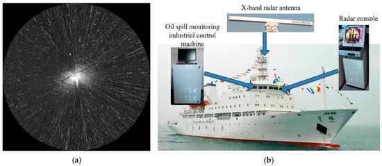
Figure 1.
Raw data collection and integration equipment. (a) Shipborne radar image. (b) Data collection and integration equipment.
2.2. Data Preprocessing
The data preprocessing flowchart is shown in Figure 2. Initially, the raw image is transformed from polar coordinates to the Cartesian coordinate system. Subsequently, the Laplacian operator convolution and Otsu thresholding were applied to segment the co-frequency interference noise. The co-frequency interference noise was further processed by using a distance-weighted filtering method. Secondly, the gray threshold and isolated target area threshold were used to extract speckle noises in the image, as shown in Figure 3a. Then, the gray level co-occurrence matrix was generated to adjust the overall gray distribution of the noise reduction image, as shown in Figure 3b. Finally, the local contrast enhancement model was used to enhance the contrast inside and outside the oil films, as shown in Figure 3c.
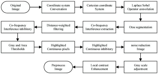
Figure 2.
The flow of data preprocessing.
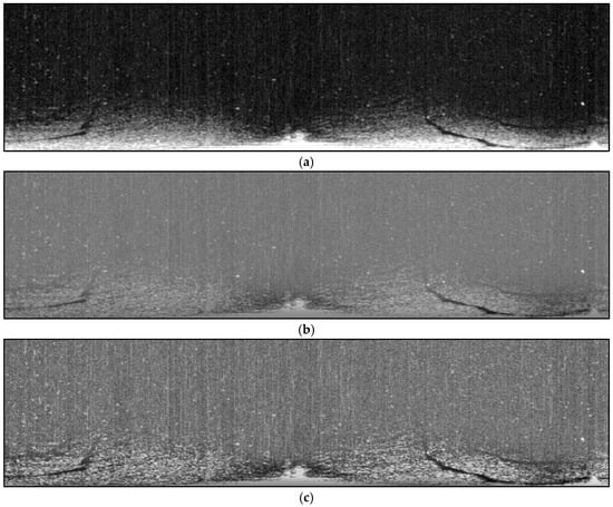
Figure 3.
Preprocessing results. (a) Noise reduction image. (b) Grayscale adjustment image. (c) Contrast enhancement image.
2.3. Texture Feature Extraction
2.3.1. Gray Level Co-Occurrence Matrix (GLCM)
The GLCM is employed as a feature extraction technique that leverages both grayscale and gradient information in an image. The GLCM represents the probability that a pixel with grayscale intensity i co-occurs with another pixel in a specific spatial relationship. This relationship was defined by a given distance d and direction (0°, 45°, 90°, or 135°) [17,30]. As a result, the computation of the GLCM can be understood through the angles shown in Figure 4.
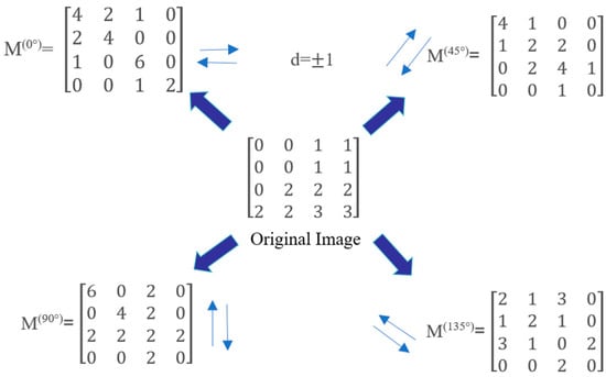
Figure 4.
Generation method of the GLCM.
Four critical texture features of the GLCM, including energy En, entropy Ent, contrast Con, and correlation Corr, were employed here as follows:
- 1.
- Energy
The energy is defined as the sum of squares of the elements in the GLCM, which serves as a metric for assessing the stability of grayscale variations in image textures. It characterizes both the uniformity of gray-level distribution and the coarseness of the texture. A high energy value indicates a regularly patterned and texturally stable region.
In this equation, p(i, j) denotes the (i, j)-th element of the normalized GLCM. N represents the number of gray levels in the image.
- 2.
- Entropy
Entropy is a statistical measure of the randomness or uncertainty associated with the information content of an image. The entropy reaches its maximum when all values in the co-occurrence matrix are equal, or when the pixel values exhibit maximal randomness. The entropy value reflects the complexity of the gray-level distribution; higher entropy indicates a more complex image.
In this equation, p(i, j)logp(i, j) represents the standard definition of information entropy. When p(i, j) equals zero, its contribution to the entropy is defined as zero.
- 3.
- Contrast
Contrast measures the distribution of values within the matrix and the degree of local variation in the image. It reflects the image sharpness and the depth of texture grooves. Deeper texture grooves result in higher contrast and a clearer visual effect. A lower contrast value indicates shallower grooves and a more blurred appearance.
In this equation, (i − j)2 denotes the squared gray-level difference, which emphasizes pixel pairs with high contrast. p(i, j) represents the elements of the GLCM.
- 4.
- Correlation
Correlation is used to measure the similarity of gray levels along the row or column direction in an image. The magnitude of the value reflects the degree of local gray-level correlation. A higher value indicates stronger correlation.
In this equation, μx and μy denote the mean gray levels of the rows and columns, respectively. σx and σy represent the standard deviations of the gray levels in the rows and columns, respectively.
2.3.2. Tamura
Tamura features exhibited robust adaptability to noise and illumination variations. The six feature components of Tamura are coarseness, contrast, directionality, roughness, line similarity, and regularity. Among them, coarseness , contrast , and directionality exhibited superior stability in texture description [31]. The above three quantitative analysis indicators were applied here to analyze image textures.
- 1.
- Coarseness
Coarseness (Fcrs) was employed to quantify the fineness or coarseness of an image. When the two texture feature patterns exhibited different primitive element sizes, the texture image with the larger primitive element pattern was determined to be coarser, whereas that with the smaller pattern was finer. Initially, the mean grayscale value was computed for each pixel as follows:
where f(i, j) represents the grayscale value of the pixel located at coordinates (i, j), Ck(x, y) denotes the average grayscale value of pixels within a specific window centered at (i, j), and l ranges from 1 to 5, which determines the size of the active window as 2l × 2l pixels. Here, it was set to 4.
Subsequently, for each pixel, the average intensity differences are computed independently for the non-overlapping windows in both the horizontal and vertical directions:
Then, coarseness (Fcrs) is determined as:
where M represents the image length and N denotes the image width. The optimal size of the window, denoted as , is obtained when E(x,y) is maximized.
- 2.
- Contrast
The contrast feature Fcon represents the grayscale difference between the brightest and darkest regions:
where denotes the fourth-order distance.
- 3.
- Directionality
The dispersion or concentration of texture along certain directions is related to the shape and arrangement regularity of texture primitives. The more irregular the image shape, the greater the range of brightness distribution and the higher the directionality. Conversely, a more regular shape results in lower directionality. It can be determined by computing the gradient vector.
First, the image was convolved with the following operators to obtain the gradient vector variations in the horizontal gradient variation ΔH and the vertical gradient variation ΔV, which can be expressed as:
Then, the gradient variation ΔG and direction angle θ for each pixel can be obtained.
Afterwards, the directional histogram HD(p) of the constructed vector is computed:
where n is the quantization interval number of the direction angle. Here, n was set to 16. p represents the index number of the p-th quantization interval. When || > t and , represents the number of edge pixels within the p-th quantization interval. is the total number of edge pixels on the corresponding direction angle θ. t is the threshold of the gradient vector mode . t was set to 12 here. Directionality Fdir can be obtained as:
where represents the index number of the quantization interval corresponding to the maximum value in the histogram HD(p). When the directionality Fdir is computed, the calculation was simplified by assuming that only one primary directional peak existed.
2.4. Feature Dimensionality Reduction
Feature dimensionality reduction methods can be categorized into linear and nonlinear approaches. Linear dimensionality reduction methods are more computationally efficient and interpretable, whereas nonlinear methods are better suited for complex data structures. Factor analysis is a classical linear dimensionality reduction method that extracts a small number of latent, unobservable common factors from a large set of observable variables. These common factors capture most of the information in the original variables, effectively simplifying the data structure and reducing dimensionality.
Factor analysis was employed for dimensionality reduction, integrating GLCM and Tamura features to generate new feature representations. The factor loading matrix was estimated using the GLS method, and factor rotation was performed with the quartic power maximum method [32]. Factor scores were evaluated using the regression estimation method.
Each feature Vi (i = 1, 2, …, p) (p = 7) in the dataset can be represented as a linear combination of common factors and a specific factor:
where F1, F2, …, Fn represent the common factors, n denotes the number of common factors, and εi is the specific factor. V can be expressed as:
Assume:
where A is the factor loading matrix, where each element aij represents the loading of feature Vi on common factor Fn, indicating their correlation coefficient. A larger absolute value signifies a stronger correlation. The key to establishing a factor analysis model for multidimensional variables V lies in solving the factor loading matrix A and the common factor vector F. The specific steps are as follows:
- 1.
- The data correlation test includes the Kaiser–Meyer–Olkin (KMO) test and sphericity of Bartlett test.
In the factor analysis, the data correlation test is a crucial step in ensuring the applicability of the factor analysis. The KMO test evaluates the correlation among variables, while the sphericity of Bartlett test determines whether the correlations among variables are significant.
The KMO test is conducted by comparing the relative magnitude of the simple and partial correlation coefficients among the original variables. When the sum of squared partial correlation coefficients among all variables is significantly smaller than the sum of squared simple correlation coefficients, the partial correlations among variables are low, and the KMO value approaches 1. The KMO value is calculated as follows:
where rij represents the simple correlation coefficient, which directly measures the linear correlation between two variables, Vi and Vj. α2ij.1,2,3…k denotes the partial correlation coefficient, which quantifies the net correlation between Vi and Vj after controlling for the influence of other variables. Clearly, when α2ij.1,2,3…k ≈ 0, the KMO value approaches 1. Conversely, when α2ij.1,2,3…k ≈ 0, the KMO value approaches 0. The KMO value ranges between 0 and 1. A dataset is deemed appropriate for dimensionality reduction using the GLS method when the KMO test value exceeds 0.60, and Bartlett’s test yields a significance p-value of less than 0.05.
- 2.
- The dataset is standardized for each eigenvalue.
To eliminate the impact of differences in scale and magnitude among variables and ensure the accuracy and reliability of the analysis, each feature Vi is standardized.
where Vi represents the feature value of a specific attribute in the dataset, μi denotes the mean of feature Vi, and σi is the standard deviation.
After standardization, each feature has a mean of 0 (μVi = 0) and a standard deviation of 1 (σVi = 1).
- 3.
- Compute the correlation matrix R = (rij) p × p.
The correlation matrix R is a p × p symmetric matrix, where each element rij represents the correlation coefficient between the ith and jth indicators:
Since the data have been standardized, the formula simplifies to:
In the equation, ri = 1, rij = rji, where rij is the correlation coefficient between the ith and jth indicators.
- 4.
- Extract the factor loading matrix using the GLS estimation method.
To extract the structural relationship between potential common factors and observed variables, the GLS method is applied to estimate the factor loading matrix. This method is based on the classical common factor analysis model, which assumes that p observed variables x = [x1, x2, …xp]T could be expressed as a linear combination of latent factors f = [f1, f2, …fm]T and an error term.
Here, Λ ϵ Rp × m denotes the factor loading matrix, which reflects the loadings of each observed variable on the common factors. The vector f represents the common factors, which are assumed to follow a standard normal distribution f~N (0, Im). The vector ϵ represents the unique factors (error terms), which were assumed to be mutually independent and follow a specific distribution ϵ~N (0, Ψ). The matrix Ψ is a diagonal matrix representing the unique variance of each variable. It is further assumed that f and ϵ are mutually independent.
Based on the above assumptions, the theoretical covariance matrix of the variables Σ can be expressed as:
In practical analysis, Σ cannot be directly obtained and can only be estimated indirectly through the sample covariance matrix S based on the observed data. The core objective of the GLS method is to estimate the parameters Λ and Ψ. These estimators are derived to minimize the discrepancy between the model-implied covariance matrix Σ and the sample covariance matrix S, subject to structural constraints. The GLS method constructs the following weighted residual sum-of-squares objective function FGLS:
Vech () denotes the vector-half operator, which vectorizes the lower triangular part of a symmetric matrix in a column-wise manner. W represents the asymptotic covariance matrix of vech(S), accounting for the correlation and heteroskedasticity among estimation errors of the covariance elements. Within the framework of GLS, incorporating W−1 enhanced the statistical efficiency and robustness of parameter estimation, particularly due to its favorable asymptotic properties in large samples.
As the objective function was nonlinear, its solution was typically obtained using numerical iterative methods. The estimation process began with the initialization of the factor loading matrix and the unique variance matrix. Common methods included PCA and eigenvalue decomposition to obtain the initial estimate of Λ(0). The initial unique variance matrix Ψ(0) was then obtained through computation:
Next, the objective function was iteratively optimized using nonlinear methods such as the quasi-Newton (e.g., Broyden–Fletcher–Goldfarb–Shanno, BFGS) or trust-region algorithms. At each iteration, Σ(k) was constructed based on the current estimates, and the residual S − Σ(k) and parameters were updated. The convergence was assessed based on predefined thresholds for the objective value or parameter changes.
After estimation, the factor loading matrix represents the linear weights of each observed variable on the common factors. It is used to interpret the underlying structural relationships among the variables. To enhance interpretability, the initial solution is typically subjected to factor rotation. This included orthogonal rotation methods, such as varimax, or oblique methods such as oblimin, which allowed for factor correlation.
- 5.
- Select q (q ≤ p) principal factors and perform factor rotation using the quartimax method.
The quartimax rotation aims to simplify the rows of the factor loading matrix by rotating the initial factors so that each variable has a high loading on only one factor while maintaining low loadings on the others. Factor interpretation is most straightforward when each variable has a nonzero loading on only one factor. The quartimax method maximizes the variance of the squared factor loadings within each row of the factor loading matrix.
The simplification criterion Q is:
The final simplification criterion Q is:
- 6.
- Compute the factor scores and complete feature fusion.
Factor scores are the most significant outcome of factor analysis. The factor loading matrix can be constructed based on the results of factor analysis. By computing the specific factor scores for each sample, the original variables can be replaced, thereby achieving dimensionality reduction.
A single factor score function was derived using the regression method.
denoted as:
Thus,
where denote, respectively, the correlation matrix of the original variables, the coefficients of the j-th factor score function, and the j-th column of the loading matrix. This can be represented in matrix form:
Then, a new feature is generated using the factor score coefficients obtained through the regression method.
2.5. Bimodal Histogram Method
The bimodal histogram method is an adaptive thresholding technique. This method involves the iterative smoothing of the image grayscale histogram. Once two local maxima appear in the histogram, indicating a typical bimodal distribution, the valley point between the peaks is selected as the segmentation threshold, as shown in Figure 5. Here, T1 and T2 represent the local peaks, and T denotes the valley threshold between them.
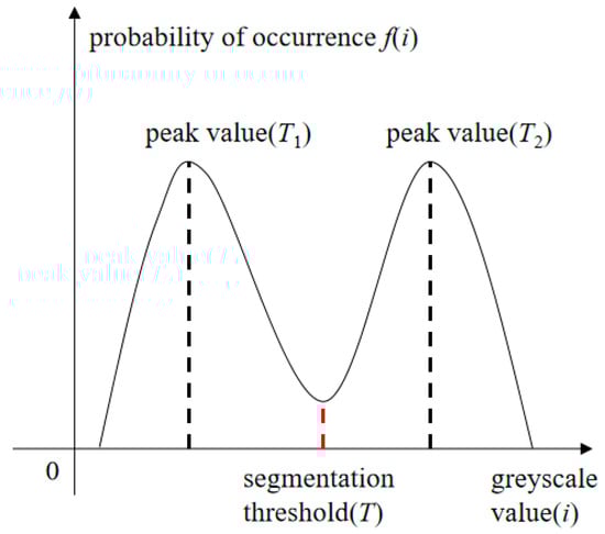
Figure 5.
Bimodal histogram threshold method.
2.6. Artificial Bee Colony Algorithm
The ABC algorithm is a metaheuristic that mimics bee colony intelligence through information sharing and cooperation. Its core idea is to balance global exploration and local exploitation through a division of labor and cooperation mechanism within the bee swarm, thereby enabling efficient solutions to complex optimization problems. The colony’s foraging system consists of employed, onlooker, and scout bees. Each type searches the solution space based on specific rules and gradually approaches the optimum through dynamic adjustment of global and local optima [33].
Employed bees are responsible for exploring new solutions within the current search space, which are then shared with onlooker bees. Onlooker bees evaluate these solutions and conduct local searches based on the better ones. Scout bees explore random regions of the solution space to ensure population diversity. Optimal solutions are identified through the collaboration among the three types of bees in the ABC algorithm [34]. The process of the ABC algorithm can be divided into the following four phases.
- 1.
- Initialization Phase
The initialization of the ABC algorithm includes two steps: parameter initialization and population initialization. Parameter initialization involves the colony size, the number of employed and onlooker bees, and the number of iterations. Population initialization is performed by generating SN feasible solutions within the solution space, each being a D-dimensional vector, with D representing the number of variables in the optimization problem. Let xi (i = 1, 2, …, SN) denote the i-th feasible solution in the population. The initialization formula is given by:
where and represent the maximum and minimum values of the j-th dimensional solution, respectively.
- 2.
- Employed Bee Phase
Employed bees search for new food sources within the neighborhood of their current position. For individual i, a new solution is generated by randomly selecting a different individual k (where k ≠ i):
where ∼ u (0,1) is a uniformly distributed random number. Boundary constraints are then applied. Afterwards, a greedy selection strategy is used to retain the elite solution:
where vij represents the continuous value of the j-th dimension of the new candidate solution, where j is the index of the threshold vector dimension. The new solution is updated only if it yields a better fitness value:
where vi indicates that f(vi) needs to be recalculated to evaluate solution quality.
Employed bees modify food sources based on their individual experience and the fitness value of the new source. When the fitness of the new source is higher than that of the old one, the old source is discarded, and the bee updates its position using the new source.
- 3.
- Onlooker Bee Phase
Employed bees share the fitness and location information of food sources with onlooker bees in the hive. Onlooker bees analyze the available information and select a food source with a certain probability:
where pi represents the probability of selecting a food source, and f(xi) denotes the fitness value of the i-th food source. A higher fitness value corresponds to a higher selection probability. Once a food source is selected, a new search is performed in its neighborhood following the same procedure used in the employed bee phase to explore solutions with improved fitness.
- 4.
- Scout Bee Phase
If the position of a food source remains unchanged for a predefined number of iterations, it is considered abandoned, and the scout bee phase is activated. In this phase, the bee associated with the abandoned source is converted into a scout bee, and the source is replaced by a new one randomly selected within the search space. When an individual fails to improve for a consecutive number of limit iterations, a random reset is triggered, and a new food source is generated to replace the old one.
3. Results and Discussion
3.1. Feature Extraction
GLCM features were extracted from Figure 3c, yielding the contrast, correlation, energy, and homogeneity feature maps using a local window of 9 × 9 pixels, as shown in Figure 6. In comparison to conventional window sizes used for texture analysis, this configuration achieved a balance between computational efficiency and feature sensitivity.
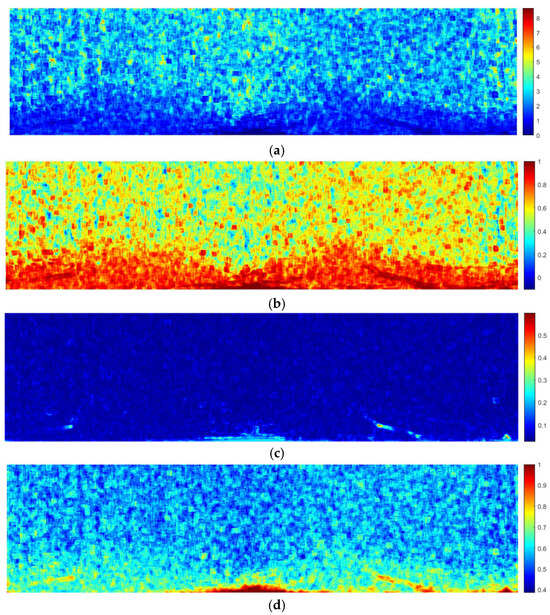
Figure 6.
GLCM feature maps. (a) Contrast. (b) Correlation. (c) Energy. (d) Homogeneity.
The size of the local window was subsequently adjusted to 19 × 19 pixels, following which a second round of local texture feature analysis was carried out on Figure 3c. As a result, feature maps for the contrast, coarseness, and directionality of Tamura were generated, as shown in Figure 7.
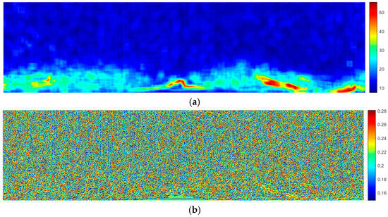
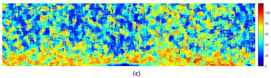
Figure 7.
Tamura feature maps. (a) Contrast. (b) Roughness. (c) Directionality.
3.2. Feature Fusion
Dimensionality reduction and the fusion of GLCM and Tamura features were achieved through factor analysis, combining the GLS method and regression estimation. The KMO value was ‘0.794’. The significance level of Bartlett’s test was less than ‘0.01’. Based on the factor scores estimated via regression, the fused feature vector FReg was obtained as follows:
Then, the feature fusion result was obtained, as shown in Figure 8.
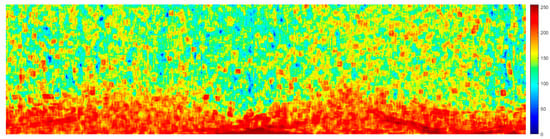
Figure 8.
Fusion feature map.
3.3. Image Threshold Segmentation
The feature fusion image was first segmented by using the histogram bimodal method, as shown in Figure 9a. Thereafter, a disk-shaped structuring element with a radius of 2 was used to expand white regions and connect adjacent areas, producing the grayscale image shown in Figure 9b. Subsequently, a region-filtering process was conducted to eliminate isolated regions. This resulted in the ocean wave region, as shown in Figure 9c,d.
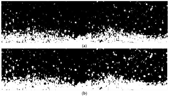
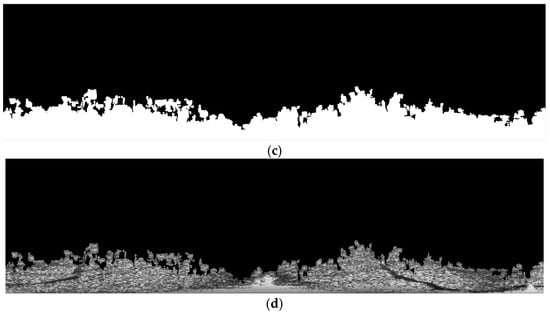
Figure 9.
Extraction of effective ocean wave areas in the marine radar image. (a) Segmentation of the fusion feature map. (b) Morphological dilation. (c) Deletion of isolated areas. (d) Segmentation of effective ocean wave areas.
3.4. Artificial Bee Colony Algorithm Segmentation
Initially, single-threshold segmentation was applied in the segmentation image of effective ocean wave areas (Figure 9d) using the ABC algorithm. The optimal threshold was determined by maximizing inter-class variance, which ensured the best separation performance. Ultimately, the image was binarized based on the obtained optimal threshold, as shown in Figure 10.
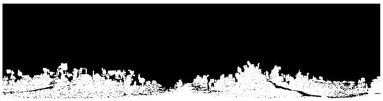
Figure 10.
Segmentation of the ABC algorithm.
3.5. Oil Spill Segmentation Mask
Firstly, small areas of noise in the segmentation of the ABC algorithm (Figure 10) with less than 50 pixels were removed. In addition, spatial constraints were applied through a mask image to eliminate located ship wake interference signals. Thereafter, the binary image was inverted to unify the representation of the target region, producing the final segmentation mask, as shown in Figure 11a. Next, a nonlinear coordinate transformation from Cartesian to polar coordinates was performed using bilinear interpolation. Polar parameters were computed by constructing an extended grid, and the segmentation result was mapped to the polar coordinate system along with the original radar image. After completing the geometric transformation, horizontal and vertical flipping were applied to the image matrix to adjust the orientation. The resulting polar coordinate image is shown in Figure 11b.
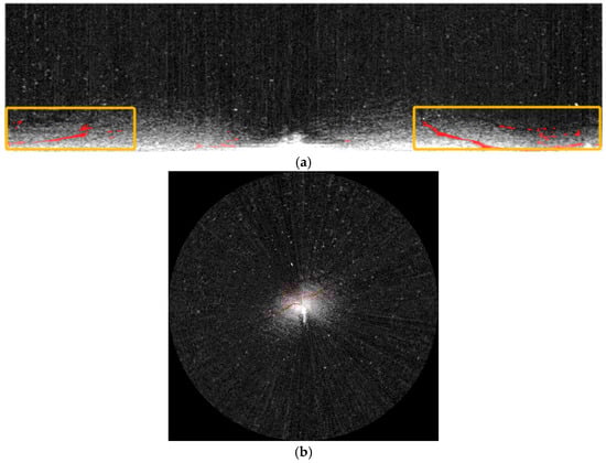
Figure 11.
Oil spill segmentation image. (a) Mask image in polar coordinates. (b) Mask image in Cartesian coordinates.
3.6. Comparison of the ABC Algorithm with Other Optimization Algorithms
Common optimization algorithms used in image processing include the Grey Wolf Optimizer, Cuckoo Search Algorithm, Whale Optimization Algorithm, etc. For the comparative analysis, the aforementioned optimization algorithms were also applied to the same image. The corresponding results are shown in Figure 12. In Figure 12a,d, some oil spill regions were accurately identified [35,36]. However, certain oil film areas remained undetected, resulting in incomplete recognition. In contrast, the results in Figure 12b,c achieved a more complete detection of oil spill regions but mistakenly classified some non-spill areas as oil-contaminated [37,38]. In particular, Figure 12b presents a result from a flight-strategy-based Grey Wolf Optimization algorithm.
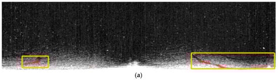
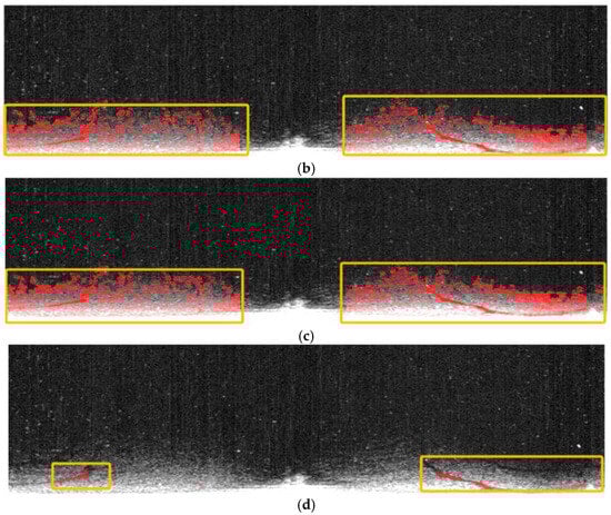
Figure 12.
The resultant images of other optimization algorithms. (a) Grey Wolf Optimization. (b) The Cuckoo Search Algorithm. (c) Grey Wolf Optimization Algorithm based on flight strategy. (d) The Whale Optimization Algorithm.
Based on a comprehensive comparison, the ABC algorithm demonstrated the best performance in terms of detection accuracy and false recognition control. It successfully identified all oil spill regions without introducing significant misclassification.
3.7. Experimental Comparison of Generalized Least Square Methods
During the feature map fusion process, PCA was introduced for dimensionality reduction to enable comparative analysis. Under consistent experimental conditions, PCA was used in place of the GLS method to generate the fused image, as shown in Figure 13a. Subsequently, the bimodal histogram method was applied to perform adaptive thresholding on the fused image, and the segmentation result is shown in Figure 13b.
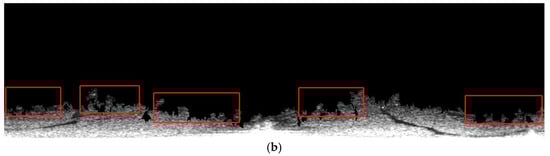
Figure 13.
Experimental images of the PCA method. (a) Feature fusion map. (b) Wave segmentation image.
The results indicated that PCA successfully identified several large oil spill regions. However, it encountered difficulty in distinguishing oil spills near sea wave boundaries, leading to inaccurate classification in some regions. In contrast, the fused image processed using GLS exhibited superior segmentation performance in such boundary regions, enabling more effective differentiation between oil spills and sea clutter.
3.8. The Comparison Between Experimental Algorithms and Deep Neural Networks
At present, relatively rich processing methods for radar images have been developed, among which image recognition technology based on deep neural networks has emerged as an important research direction. In this experiment, the YOLO object detection model was selected as the comparison benchmark. In terms of identifying oil film regions, target segmentation tasks can be accurately completed by the YOLO model, indicating its adaptability to radar image scenes. Then, as shown in Figure 14, a significant number of duplicate bounding boxes were generated by the YOLO model while predicting the oil films. The processing burden on subsequent recognition results is increased by these repetitions. In contrast, the occurrence of duplicates can be effectively reduced by the method used in our experiment, while maintaining high precision in oil film segmentation. Therefore, from a comprehensive performance perspective, the processing strategy proposed in our experiment possesses certain advantages over radar image oil film detection.
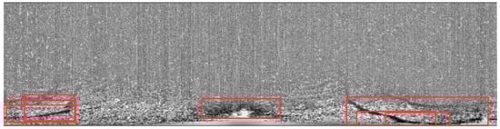
Figure 14.
YOLO processing result image.
3.9. The Influence of Different Sea Conditions on Radar Oil Spill Detection Images
Currently, shipborne radar images in the field of oil spill detection still face several limitations. The shipborne radar system detects sea surface targets through the emission of electromagnetic waves and the reception of echo signals reflected by targets. Among these factors, wave fluctuations are identified as one of the key factors affecting the accuracy of radar recognition. Shipborne radar primarily relies on differences in sea surface roughness for the identification of oil films. When an oil spill occurs on the sea surface, the attenuation effect exerted by the oil film on centimeter waves leads to a reduction in the backscatter intensity of the radar. Consequently, weaker signal characteristics are observed in the oil film area of the radar image compared to the surrounding sea areas. Under adverse sea conditions, subtle differences in surface roughness can be masked by wave fluctuations, resulting in misjudgments of natural smooth areas or missed detections of actual oil spills. As illustrated in Figure 15a, accurate identification of the oil film area becomes particularly challenging in radar images characterized by large wave fluctuations. Additionally, high-level speckle noise can be introduced by strong wave fluctuations, further complicating the precise positioning of oil spill boundaries.
Figure 15.
Radar monitoring images under different wave fluctuations. (a) Strong wave fluctuations. (b) Weak wave fluctuations.
Conversely, recognition errors may also occur under low sea conditions. As depicted in Figure 15b, in a calm sea environment, a low grayscale contrast is observed between the oil film and the background. Consequently, naturally smooth sea areas might be misjudged as oil film areas, while actual oil spills may be overlooked due to insufficient contrast. Although the oil film remains on a calm sea surface for an extended period, its thin thickness renders its chemical properties more susceptible to interference from environmental noise, thereby increasing the difficulty of monitoring.
3.10. Discussion on Outcome Indicators
Expert visual explanation requires manually drawing oil film targets. During the manual drawing process, there may be errors in the target edges. Our method of extracting oil film targets using an adaptive threshold is a type of automatic calculation method. The segmentation of the oil film target edges by the proposed method is relatively accurate.
In the expert visual interpretation process for oil film target recognition, manually drawing the oil film target is required. However, as demonstrated by the visual explanation of the expert case of the oil spill area presented in Figure 16, this manual drawing approach inevitably leads to the introduction of errors at the target edges. In contrast, the adaptive threshold extraction method for oil film targets, which is an automatic calculation method, generally results in a relatively more accurate segmentation of the oil film target’s edges. Nevertheless, this advantage in edge accuracy achieved by the automatic method is also a contributing factor to the decrease in accuracy and recall. A comparison between the method proposed by our research institute and expert explanations is illustrated in Figure 17. It was noteworthy that ship elements with medium-intensity reflections were present in the blue-outlined regions. As a result, the adaptive thresholding method was unable to effectively segment the oil film in these regions. In contrast, expert interpretations suggested that such interference from ships on the oil film can be effectively eliminated. Moreover, in the yellow-outlined regions, the oil film exhibits an extremely high similarity to the background. This leads to the inability of the adaptive threshold segmentation method to achieve satisfactory results. Meanwhile, in the green-outlined regions, the recognition results may be affected by errors due to the influence of ship wakes.
Figure 16.
Expert visual interpretation of oil spill regions.
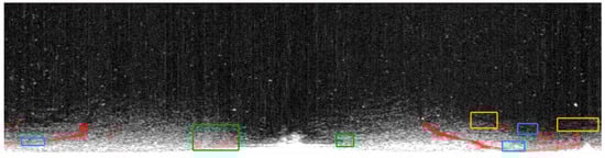
Figure 17.
Comparison between the proposed method and expert interpretation.
In summary, although some errors exist when the proposed method was compared with the expert interpretation method, accuracy, recall, and F1 scores of more than 96% were achieved, indicating that the method has yielded good results.
4. Conclusions
Oil spill detection, as a pivotal application of remote sensing technology in marine environmental monitoring, is increasingly garnering widespread attention. Characterized by its capabilities for large-scale, high-frequency, and non-contact observations, remote sensing technology has emerged as a crucial tool for monitoring marine oil spills. Although the application of shipborne radar in oil spill detection is still in its nascent stages, it demonstrates considerable potential for large-scale deployment.
In this study, we proposed an oil film segmentation method that integrates feature extraction and fusion techniques. This method was tailored to the characteristics of oil spill areas in radar images by incorporating the ABC algorithm. Initially, the acquired raw radar image was subjected to preprocessing. Subsequently, grayscale adjustment and local contrast enhancement operations were performed on the preprocessed image. Next, the GLCM and Tamura features were extracted, and feature fusion was achieved using the GLS method. Finally, wave regions were extracted using the histogram bimodal method, followed by oil film segmentation using the ABC algorithm.
The feature extraction and fusion strategy proposed in this study significantly enhances detection efficiency, while the incorporation of the GLS method facilitates more effective extraction of oil spill areas. Furthermore, the ABC algorithm was introduced for object extraction to address the limitations of traditional methods, such as sensitivity to initial data and susceptibility to local optima. Its application improved the stability and adaptability of segmentation results, thereby enhancing the accuracy of oil film segmentation.
The experimental results indicated that high segmentation accuracy and robustness were achieved by this method, suggesting its potential for application in complex environments. However, current methods still exhibit certain limitations when processing images with extremely low contrast or strong interfering backgrounds. These limitations may lead to misclassification or blurred boundaries. Additionally, when the sea surface is unusually calm, the lack of sufficient roughness can also render the identification of the oil film difficult. Moreover, under strong wind conditions, the intense mixing of oil spills with seawater can cause the oil film to be dispersed or diluted, thereby increasing the difficulty of distinguishing the characteristics of oil spills. These situations often lead to inaccurate classification and unclear definitions of object boundaries, thus compromising the reliability of segmentation results in challenging visual scenes. The future research direction will focus on realizing real oil film segmentation in various radar scenarios, sea conditions, types of oil, and radar system environments.
Author Contributions
Conceptualization, J.X. and B.X.; methodology, J.X., B.X. and X.M.; software, B.Y. and Z.G.; validation, B.Y. and X.W.; formal analysis, Y.H., S.Q. and M.C.; investigation, J.X., B.X. and B.Y.; resources, J.X., S.Q. and M.C.; data curation, J.X. and X.M.; writing—original draft preparation, B.X. and J.X.; writing—review, P.L. and X.M.; visualization, B.X.; supervision, Z.G. and J.W.; project administration, X.M. and J.X.; funding acquisition, X.M. and J.X. All authors have read and agreed to the published version of the manuscript.
Funding
This research was supported by the Guangdong Basic and Applied Basic Research Foundation, grant numbers 2025A1515010886 and 2023A1515011212, the Special Projects in Key Fields of Ordinary Universities in Guangdong Province, grant number 2022ZDZX3005, the Shenzhen Science and Technology Program, grant number JCYJ20220530162200001, the Postgraduate Education Innovation Project of Guangdong Ocean University, grant number 202421, the Guangdong Provincial Key Laboratory of Intelligent Equipment for South China Sea Marine Ranching, grant number 080508132401.
Data Availability Statement
The data collection department did not agree to share the analysis data.
Acknowledgments
During the preparation of this manuscript, the authors used Chat GPT-4o for the purposes of polishing the language in the Section 2. The authors have reviewed and edited the output and take full responsibility for the content of this publication.
Conflicts of Interest
The authors declare no conflicts of interest.
References
- Fan, J.; Liu, C. Multitask GANs for Oil Spill Classification and Semantic Segmentation Based on SAR Images. IEEE J. Sel. Top. Appl. Earth Obs. Remote Sens. 2023, 16, 2532–2546. [Google Scholar] [CrossRef]
- Ma, Y.; Medini, P.C.P.; Nelson, J.R.; Wei, R.; Grubesic, T.H.; Sefair, J.A. A Visual Analytics System for Oil Spill Response and Recovery. IEEE Comput. Graph. Appl. 2021, 41, 91–100. [Google Scholar] [CrossRef]
- Chen, F.; Zhang, A.; Balzter, H.; Ren, P.; Zhou, H. Oil Spill SAR Image Segmentation via Probability Distribution Modeling. IEEE J. Sel. Top. Appl. Earth Obs. Remote Sens. 2022, 15, 533–554. [Google Scholar] [CrossRef]
- Chen, G.; Huang, J.; Wen, T.; Du, C.; Lin, Y.; Xiao, Y. Multiscale Feature Fusion for Hyperspectral Marine Oil Spill Image Segmentation. J. Mar. Sci. Eng. 2023, 11, 1265. [Google Scholar] [CrossRef]
- Li, Y.; Lyu, X.; Frery, A.C.; Ren, P. Oil Spill Detection with Multiscale Conditional Adversarial Networks with Small-Data Training. Remote Sens. 2021, 13, 2378. [Google Scholar] [CrossRef]
- Yang, J.; Wang, J.; Hu, Y.; Ma, Y.; Li, Z.; Zhang, J. Hyperspectral Marine Oil Spill Monitoring Using a Dual-Branch Spatial–Spectral Fusion Model. Remote Sens. 2023, 15, 4170. [Google Scholar] [CrossRef]
- Adamu, B.; Tansey, K.; Ogutu, B. An investigation into the factors influencing the detectability of oil spills using spectral indices in an oil-polluted environment. Int. J. Remote Sens. 2016, 37, 2338–2357. [Google Scholar] [CrossRef]
- Mohamadi, B.; Liu, F.; Xie, Z. Oil Spill Influence on Vegetation in Nigeria and Its Determinants. Pol. J. Environ. Stud. 2016, 25, 2533–2540. [Google Scholar] [CrossRef] [PubMed]
- Sun, H.; Ma, L.; Fu, Q.; Li, Y.; Shi, H.; Liu, Z.; Liu, J.; Wang, J.; Jiang, H. Long-Wave Infrared Polarization-Based Airborne Marine Oil Spill Detection and Identification Technology. Photonics 2023, 10, 588. [Google Scholar] [CrossRef]
- Li, Z.; Johnson, W. An Improved Method to Estimate the Probability of Oil Spill Contact to Environmental Resources in the Gulf of Mexico. J. Mar. Sci. Eng. 2019, 7, 41. [Google Scholar] [CrossRef]
- Asif, Z.; Chen, Z.; An, C.; Dong, J. Environmental Impacts and Challenges Associated with Oil Spills on Shorelines. J. Mar. Sci. Eng. 2022, 10, 762. [Google Scholar] [CrossRef]
- Duan, P.; Kang, X.; Ghamisi, P.; Li, S. Hyperspectral Remote Sensing Benchmark Database for Oil Spill Detection with an Isolation Forest-Guided Unsupervised Detector. IEEE Trans. Geosci. Remote Sens. 2023, 61, 5509711. [Google Scholar] [CrossRef]
- Li, B.; Xu, J.; Pan, X.; Chen, R.; Ma, L.; Yin, J.; Liao, Z.; Chu, L.; Zhao, Z.; Lian, J.; et al. Preliminary Investigation on Marine Radar Oil Spill Monitoring Method Using YOLO Model. J. Mar. Sci. Eng. 2023, 11, 670. [Google Scholar] [CrossRef]
- Xu, J.; Pan, X.; Jia, B.; Wu, X.; Liu, P.; Li, B. Oil Spill Detection Using LBP Feature and K-Means Clustering in Shipborne Radar Image. J. Mar. Sci. Eng. 2021, 9, 65. [Google Scholar] [CrossRef]
- Xu, J.; Qian, W.; Chen, Q.; Gu, G.; Lu, Y.; Zhou, Y. Uniform Scattering Power for Monitoring the Spilled Oil on the Sea. IEEE Photonics J. 2018, 10, 6100310. [Google Scholar] [CrossRef]
- Gong, B.; Mao, S.; Li, X.; Chen, B. Mineral Oil Emulsion Species and Concentration Prediction Using Multi-Output Neural Network Based on Fluorescence Spectra in the Solar-Blind UV Band. Anal. Methods 2024, 16, 1836–1845. [Google Scholar] [CrossRef]
- Li, B.; Xu, J.; Pan, X.; Ma, L.; Zhao, Z.; Chen, R.; Liu, Q.; Wang, H. Marine Oil Spill Detection with X-Band Shipborne Radar Using GLCM, SVM and FCM. Remote Sens. 2022, 14, 3715. [Google Scholar] [CrossRef]
- Hou, Y.; Li, Y.; Liu, B.; Liu, Y.; Wang, T. Design and Implementation of a Coastal-Mounted Sensor for Oil Film Detection on Seawater. Sensors 2018, 18, 70. [Google Scholar] [CrossRef]
- Du, K.; Ma, Y.; Li, Z.; Liu, R.; Jiang, Z.; Yang, J. MS3OSD: A Novel Deep Learning Approach for Oil Spills Detection Using Optical Satellite Multisensor Spatial-Spectral Fusion Images. IEEE J. Sel. Top. Appl. Earth Obs. Remote Sens. 2025, 18, 8617–8629. [Google Scholar] [CrossRef]
- Yang, J.; Ma, Y.; Hu, Y.; Jiang, Z.; Zhang, J.; Wan, J.; Li, Z. Decision Fusion of Deep Learning and Shallow Learning for Marine Oil Spill Detection. Remote Sens. 2022, 14, 666. [Google Scholar] [CrossRef]
- Iordache, M.-D.; Viallefont-Robinet, F.; Strackx, G.; Landuyt, L.; Moelans, R.; Nuyts, D.; Vandeperre, J.; Knaeps, E. Feasibility of Oil Spill Detection in Port Environments Based on UV Imagery. Sensors 2025, 25, 1927. [Google Scholar] [CrossRef]
- Ji, M.; Yuan, Y. Dimension Reduction of Image Deep Feature Using PCA. J. Vis. Commun. Image Represent. 2019, 63, 102578. [Google Scholar] [CrossRef]
- Wang, Z.; Liang, S.; Xu, L.; Song, W.; Wang, D.; Huang, D. Dimensionality reduction method for hyperspectral image analysis based on rough set theory. Eur. J. Remote Sens. 2020, 53, 192–200. [Google Scholar] [CrossRef]
- Zhao, W.; Du, S. Spectral—Spatial Feature Extraction for Hyperspectral Image Classification: A Dimension Reduction and Deep Learning Approach. IEEE Trans. Geosci. Remote Sens. 2016, 54, 4544–4554. [Google Scholar] [CrossRef]
- Li, H.; Cui, J.; Zhang, X.; Han, Y.; Cao, L. Dimensionality Reduction and Classification of Hyperspectral Remote Sensing Image Feature Extraction. Remote Sens. 2022, 14, 4579. [Google Scholar] [CrossRef]
- Zhao, C.; Zhao, H.; Wang, G.; Chen, H. Improvement SVM Classification Performance of Hyperspectral Image Using Chaotic Sequences in Artificial Bee Colony. IEEE Access 2020, 8, 73947–73956. [Google Scholar] [CrossRef]
- Zhi, H.; Liu, S. Gray Image Segmentation Based on Fuzzy C-Means and Artificial Bee Colony Optimization. J. Intell. Fuzzy Syst. 2020, 38, 3647–3655. [Google Scholar] [CrossRef]
- Huo, F.; Wang, Y.; Ren, W. Improved artificial bee colony algorithm and its application in image threshold segmentation. Multimed. Tools Appl. 2022, 81, 2189–2212. [Google Scholar] [CrossRef]
- Chen, J.; Yu, W.; Tian, J.; Chen, L.; Zhou, Z. Image Contrast Enhancement Using an Artificial Bee Colony Algorithm. Swarm Evol. Comput. 2018, 38, 287–294. [Google Scholar] [CrossRef]
- Li, K.; Yu, H.; Xu, Y.; Luo, X. Detection of Oil Spills Based on Gray Level Co-Occurrence Matrix and Support Vector Machine. Front. Environ. Sci. 2022, 10, 1049880. [Google Scholar] [CrossRef]
- Kong, L.J.; He, Q.; Liu, G.H. Image retrieval based on deep Tamura feature descriptor. Multimed. Syst. 2024, 30, 148. [Google Scholar] [CrossRef]
- Li, C.; Evans, D.J. GSOR Method for the Equality Constrained Least Squares Problems and the Generalized Least Squares Problems. Int. J. Comput. Math. 2002, 79, 955–960. [Google Scholar] [CrossRef]
- Coskun, O.; Ozturk, C.; Sunar, F.; Karaboga, D. The Artificial Bee Colony Algorithm in Training Artificial Neural Network for Oil Spill Detection. Neural Netw. World 2011, 21, 473–492. [Google Scholar] [CrossRef]
- Ning, J.; Liu, T.; Zhang, C.; Zhang, B. A food source-updating information-guided artificial bee colony algorithm. Neural Comput. Appl. 2018, 30, 775–787. [Google Scholar] [CrossRef]
- Fu, Y.; Xiao, H.; Lee, L.H.; Huang, M. Stochastic Optimization Using Grey Wolf Optimization with Optimal Computing Budget Allocation. Appl. Soft Comput. 2021, 103, 107154. [Google Scholar] [CrossRef]
- Liu, L.; Zhang, R. Multistrategy Improved Whale Optimization Algorithm and Its Application. Comput. Intell. Neurosci. 2022, 2022, 3418269. [Google Scholar] [CrossRef] [PubMed]
- Rajabioun, R. Cuckoo Optimization Algorithm. Appl. Soft Comput. 2011, 11, 5508–5518. [Google Scholar] [CrossRef]
- Heidari, A.A.; Parham, P. An Efficient Modified Grey Wolf Optimizer with Lévy Flight for Optimization Tasks. Appl. Soft Comput. 2017, 60, 115–134. [Google Scholar] [CrossRef]
Disclaimer/Publisher’s Note: The statements, opinions and data contained in all publications are solely those of the individual author(s) and contributor(s) and not of MDPI and/or the editor(s). MDPI and/or the editor(s) disclaim responsibility for any injury to people or property resulting from any ideas, methods, instructions or products referred to in the content. |
© 2025 by the authors. Licensee MDPI, Basel, Switzerland. This article is an open access article distributed under the terms and conditions of the Creative Commons Attribution (CC BY) license (https://creativecommons.org/licenses/by/4.0/).