Abstract
Halifax Harbour, a major seaport in Nova Scotia that is approximately 100 km southeast of the Bay of Fundy, comprises a deep inner region called Bedford Basin, connected to the adjacent ocean by a shallow channel called The Narrows. A study of sea level and currents reveals the presence of episodic oscillations in The Narrows, with a period of approximately 2 h. The oscillation strength varies from day to day and, to some extent, through the seasons. The median amplitude of the associated sea level variation is that of the de-tided signal, rising to at the 95-th percentile. Values this large may be of concern for the transit of deep-draft vessels through shallow parts of the harbour and for the clearance of tall vessels under the two bridges that span The Narrows. Another concerning issue is the matter of oscillations being superimposed on storm surges. In addition to such direct effects of sea level variation, shear associated with the oscillations may increase the turbulent mixing in the region, affecting the overall state of this estuarine system. We explore the nature of the oscillations as a first step towards the improvement of prediction schemes for sea level and currents in the region. This involves an analysis of the oscillations in the context of seiche and Helmholtz resonance theories and the use of a 2D numerical model to handle realistic bathymetric conditions and other complications that the simpler theories cannot address. We conclude that the predictions of Helmholtz resonance theory are in reasonable agreement with both the observations and the predictions of the numerical model.
1. Introduction
Halifax Harbour (Figure 1) is one of the world’s largest deep-water harbours and is of prime military and commercial importance to Canada [1]. Early European explorers found the coastal region to be seasonally occupied by the Indigenous peoples now known as the Mi’kmaq, who moved inland for game hunting in wintertime, returning to the coast in the summer for fishing. This pattern of seasonal occupation has been postulated to have extended back to the last ice age [2], when reduced sea levels would have meant that what is now the saltwater Bedford Basin was a coastal lake [3].
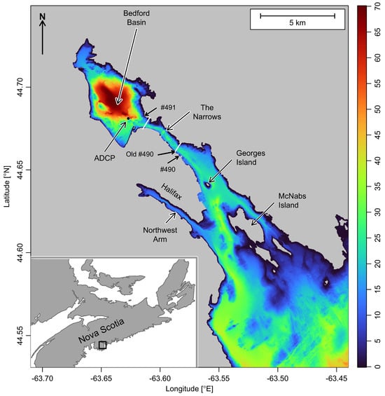
Figure 1.
Study region showing the bathymetry of Halifax Harbour and its location in the Canadian province of Nova Scotia (inset). In the main diagram, colour represents depth in metres, relative to mean sea level, based on high-resolution mapping at a nominal 10 m scale, after adjusting the reference level (see text). Some place names are noted for reference in the text. The MacKay and Macdonald bridges crossing The Narrows are indicated by white lines, with the former being near the entrance to Bedford Basin. A dot indicates the location of an acoustic Doppler current profiler, and arrows indicate the locations of present-day tide gauges #490 and #491, as well as the “Old #490” tide gauge that provided data from 1895 to 2014.
We lack a written history of the region for pre-colonial times, but the record starts to fill in during the early 1600s (see [4] for an expansive treatment). Although Halifax Harbour was not favoured for early European settlement, the French explorer Samuel de Champlain was aware of it (then called Chebucto, after the Mi’kmaq word Kjipuktuk), declaring it a good and safe harbour in the early 1600s. Through the next century, French and English influences on the region grew stronger, partly reflecting conflicts in Europe. Halifax Harbour became an important military element during that time, and it has remained so through the two World Wars [4] and up to the present day, as the Atlantic base of the Royal Canadian Navy.
As a key port on Canada’s Atlantic coastline, Halifax Harbour was the site of some of the earliest tidal measurements and analyses in Canadian waters [5,6]. Archival records hold measurements made from 1895 to 2014 at the site marked “Old #490” on Figure 1. A new tide gauge identified as #491, located near the entrance to the Bedford Basin, started reporting regularly in 2006 and continues today. In early 2024, a newer site, designated #490, was placed near the Old #490 site.
Efforts are underway to combine these tidal datasets, and these may benefit from exploration of the dynamics of the system as a whole. This is one motivation for the present analysis of the one-year period, from March 2024 to March 2025, in which high-quality data have been available at both #490 and #491. A feature of particular interest is the evidence of high-frequency (∼2 h) oscillations in sea level (Figure 2) that have amplitudes that may be relevant to shipping and, via mixing consequences, to the overall state of the harbour’s estuarine circulation. This short oscillation period being inconsistent with direct tidal and atmospheric forcing, our thoughts turned to alternative mechanisms, including seiches and Helmholtz resonances. This paper outlines some of our results. The format is as follows. Section 2 contains a sketch of our materials and methods, subdivided into subsections for data collection and analysis (Section 2.1), the theory of seiche and Helmholtz resonances (Section 2.2), and the use of a 2D numerical ocean model that provides additional insights on the Helmholtz mechanics (Section 2.3). Section 3 presents the results of our work, again subdivided into sections dealing with observation (Section 3.1), seiche and Helmholtz resonance (Section 3.2), and numerical modelling (Section 3.3). And, finally, in Section 4 we discuss our findings and present some initial conclusions.
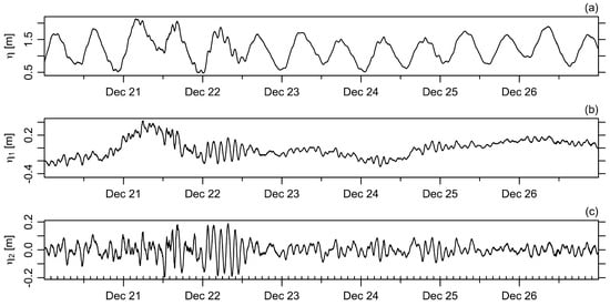
Figure 2.
Water levels observed during a week in December 2024, at tide gauge #491, near the entrance to Bedford Basin. (a) Raw signal, . (b) As (a), but minus the tidal signal. (c) As (b), but minus a smoothing cubic spline with 3 knots per day to remove effects of daily atmospheric forcing without removing the oscillation signals. In this panel, ticks indicate 2 h increments. Note that the panels have differing vertical scales to improve signal visibility.
2. Materials and Methods
2.1. Observations
All data processing and figure preparation were performed in version 4.5 of the R language [7,8], using purpose-written code [9] and relying on a variety of R packages [10], as noted below. Many choices were made in framing this code (e.g., smoothing properties for spectral computations and decisions about approximating complex bathymetry with simple models), and care was taken to find reasonable values for the relevant parameters and to check on the sensitivity of the results to these choices, as will be described later.
Bathymetry data were downloaded in the NONNA (non-navigational) format from the Canadian Hydrographic Service (CHS) website [11]. The highest-resolution datasets were selected, yielding approximately 10 m between samples. The NONNA values are defined with respect to a Chart Datum that is below mean (de-tided) sea level, and so m was added to the NONNA value to calculate water depth. The results were then averaged onto a grid (with easterly and northerly spacings of 21 m and 23 m) using the binMean2D function of the oce R package [12]. A terrain-following coordinate system was devised for the region of The Narrows to facilitate the determination of mean water depth and cross-sectional area in the channel.
Sea level data, along with associated tidal predictions, were downloaded from the Department of Fisheries and Oceanography (DFO) website [13] using the dod R package [14]. The webserver limits downloads of data sampled at a 1 min resolution to subsets of at most 1-week intervals, so the concatenate function of the oce package was used to assemble 1-year datasets. Tide gauge #491 provides several years of data, but #490 only has data starting in March of 2024, so the latter date was chosen as the start of the 1-year window examined in this study.
Spectral analysis of the sea level time series employed the smoothed-periodogram method provided by the spectrum function of the stats R package (version 4.5.0), using a modified Daniell filter with the spans parameter equal to for the smoothing. This yielded an effective bandwidth of cph, i.e., times the difference in and frequencies. See Chapter 4 of [15] for more on smoothing procedures, and spectral analysis in R, generally. Cross-spectral analysis was performed with the mvspec function of the astsa R package [16], with the same smoothing parameters as were used for the single-component case. A frequency–time diagram was constructed by splitting the data into 1-day segments and then computing spectra with spans set to , yielding an effective bandwidth of cph, i.e., 21 times the difference between the and frequencies.
The acf function of the stats R package was used for lagged autocorrelation function (ACF) analysis of sea level data subdivided into 1-day intervals and high-pass-filtered by subtracting a smoothing spline with 4 knots per semidiurnal period. This removed tidal variations as well as those associated with atmospheric effects. The oscillation period for each subinterval was then found by first-differencing the autocorrelation function, linearly interpolating, and using the uniroot.all function of the rootSolve R package [17] to isolate the first peak at nonzero lag.
Complex demodulation [18] of the sea level time series was performed by first multiplying the data by , where i is , is the target frequency, and t is time. The real and imaginary parts of the result were then smoothed with the filtfilt function of the signal R package [19] using a fourth-order low-pass Butterworth filter created by the butter function of that same package, with a cutoff frequency yielding quarter-power at a period of h.
An acoustic Doppler current profiler (ADCP) was deployed from 2023-11-24 to 2024- 04-15 (a period that only overlaps that of the sea level data used here, so we do not report on direct comparisons of the two datasets) in Bedford Basin near the sill connecting it with The Narrows (Figure 1). The device, a 600 MHz Teledyne-RDI Workhorse Sentinel II, sampled m bins at 1 Hz, reporting a 5 min ensemble every 20 min. Based on an analysis of the covariance of the horizontal components of velocity, the coordinates were rotated to align with the direction of The Narrows. The data were screened according to typical data processing guidelines [20], which include removing near-surface samples that are subject to side-lobe interference along with samples that have low correlation, high error velocity, or low backscatter. Generally, the data quality was worse in the upper portion of the water column than in the lower portion, so the present analysis is focussed on data acquired in a zone from slightly above the bottom to 12 m below the surface. After filling short gaps by interpolating linearly in time, frequency spectra of the channel-aligned velocity component were calculated using the same procedure as that employed for the sea level data, with the spans parameter set to , yielding an effective bandwidth of cph.
Computation of the propagation of numerical uncertainties was carried out with the propagate R package [21], which employs a combination of Monte Carlo simulations, Taylor expansion methods, and other schemes to trace uncertainties through analytic formulae (see, e.g., [22]).
2.2. Theory
2.2.1. Seiche Resonance
Seiches, which involve the sloshing of water in enclosed or semi-enclosed domains (see, e.g., Chapter 2 of [23]) may be the first phenomenon that comes to mind in harbour oscillations. According to Merrian’s formula (see, e.g., Section 5.8 of [24] for a review, or [25] for an early treatment), the oscillation period in a rectangular-prism domain that is open to a wider domain at one end is given by
where g represents the acceleration due to gravity, H the water depth, and L the lateral extent in the direction of sloshing. This equation is for the mode of lowest frequency, with modes of higher frequency having the 4 replaced with , where n is a positive integer indicating the mode number.
2.2.2. Helmholtz Resonance
Helmholtz resonance can occur in physical systems in which a semi-isolated domain is connected to a larger domain through a constriction (Helmholtz’s study was related to musical tone; see [26] for an English translation of his 1877 German book). Such a model was used in a detailed study of Lunenburg Harbour [27], which is located 70 km southwest of Halifax. In the present case, the semi-isolated domain is Bedford Basin, and the constriction is the region comprising The Narrows and nearby waters of the outer harbour.
Simplifying the bathymetry, we consider a deep bay of surface area A that is connected to a large exterior region by a rectangular-prism channel that has length l and cross-sectional area a, through which water flows at velocity .
Using to denote sea level in the exterior domain, and to denote sea level in the bay (the latter assumed to be spatially constant for a deep basin in which sea-level signals are spread relatively rapidly by long gravity waves), we may write a volume-averaged linear momentum equation as
The first term on the right-hand side of this equation represents the pressure-gradient force per unit mass, using the hydrostatic pressure relation, and the second term is a linearized representation of bottom friction, with representing a timescale for frictional decay of motion. (It is worth noting that Equation (2) could be extended by adding a lateral friction term that is also linear in u).
Here, the value of r will be inferred using
where is a quadratic friction coefficient, is the background speed, and h is water depth within the channel (see, e.g., Section 9.6 of [24] for a general introduction). Note that l and h in Equations (2) and (3) refer to the channel, as opposed to L and H in Equation (1), where they refer to the larger domain. Linearizing the bottom friction term for combined oscillatory and mean flows in coastal and continental shelf environments has been considered by several authors, initially in 1D [28] and later in 2D [29,30], with each treatment applying to the case of weak mean flow. Subsequently, this early work was extended to include arbitrary values of the ratio of mean speed to oscillatory flow amplitude and to arbitrary relative directions of the mean and oscillatory velocities [31]. One of the results of this last study was that Equation (3) is a reasonable approximation to an equation with fewer assumptions and that the numerical factor of 2 holds over a larger range of the ratio of the magnitudes of u to than had been discussed in the earlier literature. (See Figure 1 and Equations (3.7) and (3.8) in [31], noting that and u in the present treatment correspond to and in [31].)
With these statements about momentum, we now turn to conservation of mass. For this, we use an integrated form of the continuity equation, yielding
where A is the area of the basin into which water flows via the channel and a is the cross-sectional area of that channel. If, for convenience, we define
and
then combining Equations (2)–(4) yields a constant-coefficient differential equation for the velocity in the channel,
This may be recognized as the equation for an unforced damped simple harmonic oscillator with resonance at and damping parameter (see, e.g., Section 2.9 in [32]). Substituting as a trial solution for the case with at , we find that must satisfy
where the first term on the right-hand side yields exponential decay of the response and the second term yields a different physical character to the solutions, depending on the relative magnitudes of and .
If , i.e., in the low-friction case, the second term in Equation (8) is imaginary, indicating that the solution is oscillatory, with frequency
The forced case may be addressed by replacing the zero in Equation (7) with , where has units of velocity and is the frequency of forcing, and then seeking a trial solution , where is a complex number to be determined.
Solving the resultant algebraic equation reveals the gain , i.e., the ratio of response amplitude to forcing amplitude, to be
In a system with no friction, i.e., with , Equation (10) predicts a spike response at resonance, where . With friction, however, the peak spreads to nearby frequencies. A measure of the spread is called the quality factor, Q, defined as the ratio of resonant frequency to the span between nearby frequencies at which G is half its peak value.
The model parameters used in the rest of this paper are given in Table 1. The geometrical parameters A, a, l, and h were estimated by simplifying the bathymetry illustrated in Figure 1 and Figure 3. The basin area, A, was estimated as the area to the northwest of the MacKay bridge, near the tide gauge. The channel length, l, was taken to be the distance in The Narrows from its connection to Bedford Basin (taken as the zero of axial distance in Figure 3) to a spot near Georges Island, where the harbour widens significantly and starts to deepen and where flow will be split by the island. The channel depth, h, was taken to be the average depth in the region up to the axial distance l from Bedford Basin. The channel area, a, at the connection with Bedford Basin was inferred as the average cross-sectional area for the region of The Narrows within km of Bedford Basin.

Table 1.
Nominal values of base parameters use in the seiche and Helmholtz analyses. Other dynamical parameters are derived from these values, e.g., the friction coefficient r is from Equation (3).
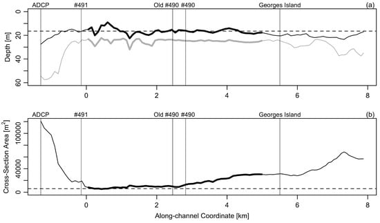
Figure 3.
Variation in depth and cross-sectional area for sections that are orthogonal to the channel axis. The zero of the along-channel coordinate is taken as the location where the channel connects with Bedford Basin. Labels atop both panels indicate some place names, for reference to Figure 1. (a) Mean depth (black line) and maximal depth (gray line), with lines thickened in the region (of length l) taken to represent the channel in the Helmholtz calculation. The dotted line is the value of h shown in Table 1 and used in the calculations. (b) Cross-sectional area, again with a thickened line in the region taken to be the channel. The dashed line is the average area (taken as a in Table 1) computed for the region within half a kilometer of Bedford Basin.
The linear bottom-drag law of Equation (3) requires knowledge of the drag coefficient, , and a representative background speed, . Each of these requires some explanation. Starting with , we relied on three published studies of coastal turbulence. The first is a report [33] on the analysis of turbulence in a tidal channel of the Bay of Fundy, 232 km west of Halifax. Table 3.3 of that report lists estimates at 4 stations, categorized by the phase of the tide. We averaged values across the stations to infer representative values of and for flood and ebb conditions, respectively. The second is a study [27] of Lunenburg Harbour, 70 km to the southwest of Halifax, which noted that models matched observations best for ranging between and . And the third is a study of turbulence in the coastal waters of the East China Sea [34] that explored the dependence of on a turbulent Reynolds number. Using data provided in a supplement to [34], and restricting attention to the putative range of the Reynolds number in the present application, reveals that the 10-th and 90-th percentiles of are and , respectively. Taking these three studies into account and averaging the low and high limits suggests that an appropriate value for the present application is , as reported in Table 1. To develop an estimate of the background current speed, , we first noted that our ADCP data are not pertinent, because they represent currents in Bedford Basin, not in the channel. Given this, we relied instead on two studies of tidal flows in the channel. The first is a report on current-meter observations made in The Narrows in 1970 [35]. An examination of diagrams in this report suggests an average current of approximately m/s. Noting that mean currents are much smaller than tidal currents in this domain, a second estimate was made using the predictions of the WebTide tidal model [36,37] in the region of The Narrows near the current-meter observations. This yielded m/s. Taking these two values as a range, and multiplying by to convert the mean speed to the standard deviation of velocity for a sinusoidally varying signal in order to express Equation (3) in the terms used by [31], we infer m/s.
The sensitivity of the predicted Helmholtz resonant period to the values of the parameters a, A, l, , U, and h was estimated by computing partial derivatives of with respect to each parameter and multiplying by half the uncertainty range of that parameter, taken as the ± value listed in Table 1 or as 10% of the value, if no ± value is listed. This is a one-at-a-time method, designed to find individual sensitivities [38]; note that a more sophisticated method that accounts for cross-dependencies will be used to find the overall uncertainty in the computed resonance period.
2.3. Two-Dimensional Numerical Model with Realistic Bathymetry
To explore some possible effects on the resonance relating to the complex bathymetry in the region, the results of theoretical calculations were compared with simulations made with a 3D numerical model called General Estuarine Transport Model (GETM) [39,40]. This model may be configured to simulate stratified flows, but for the present purpose relating to water level variations, the simulations were run in a 2D, depth-integrated mode. The horizontal resolution was degrees of both latitude and longitude, corresponding to approximately 33 m in the north–south direction and 24 m in the east–west direction. This resolution yields 10 grid cells across the narrowest portions of the harbour, which we judge to be sufficient to capture relevant motions. The initial state was set up to have zero surface elevation and zero velocity throughout the domain. The model was integrated forward in time without atmospheric forcing or riverine input. To investigate the oscillatory response, the sea level at the model boundary near McNabs Island was varied sinusoidally in time, using the “clamped elevation” GETM option. (Our choice to excite the model at this location and in this way should not be inferred as a suggestion for the forcing in the actual harbour. Rather, it is simply a convenient way to excite a response from which we can build up a gain function akin to Equation (10) for the Helmholtz theory.) Each model run had a fixed forcing period, and tests were performed with periods ranging from 1 h to 5 h. The resonance response, or gain function, was inferred as the ratio of the predicted sea level response near tide gauge #491 to the amplitude of the boundary forcing. A cyclic steady state was typically achieved after about 12 h of simulation time, so the simulations were run to 24 h, with the final two oscillation cycles being extracted for analysis.
3. Results
3.1. Observations
As noted at the outset, Figure 2 is an illustration of sea level oscillations in the channel region (at tide gauge #491). A half-dozen oscillations are clearly visible during the first half of December 22, indicating a period of about 2 h. In this case, the signal is clear and energetic, with an amplitude of approximately m, or about half the tidal amplitude. Less prominent signals of a similar period are seen throughout the week, displayed in Figure 2, and in other weeks of this year (not shown).
Spectra for tide gauges #491 and #490 (Figure 4) reveal that there is energy in a band from approximately h to h, i.e., consistent with the oscillations seen in time series, in addition to the expected tidal components in the diurnal (≈24 h), semidiurnal (≈12 h), and overtide (≈6 h) bands.
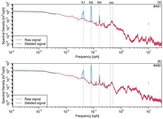
Figure 4.
Power spectra of sea level measured at tide gauges #491 and #490 (panels a,b), showing both the observed spectrum and the result of removing a tidal fit. Several tidal constituents are labelled, along with a region labelled “osc” that indicates variations with periods between h and h. The mark made at 10 cph, near the middle of the plot area, is a cross with width indicating the bandwidth and height indicating the 95% confidence interval for spectral density; the bandwidth is so small that the cross appears as a line.
Spectra of velocities measured with the ADCP moored in Bedford Basin near its connection with The Narrows also reveal a peak at periods near 2 h (Figure 5). Another feature, not explored further here, is that the flow is less sheared in this band than it is in adjacent bands and also the tidal bands. ADCP data within the channel, and over longer time periods, would be useful in follow-up work, but for now, we have verification of velocity oscillations at frequencies consistent with the oscillations in sea level.
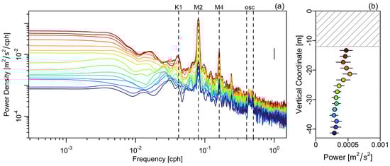
Figure 5.
Depth-dependence of the spectrum of water velocity in Bedford Basin. (a) Spectra for depths at 2 m intervals, colour-coded by depth, as indicated in the second panel. As in Figure 4, the bandwidth and confidence interval are indicated at frequency cph and power density /. (b) Spectral power in the oscillation band as a function of height above the mean sea level. The horizontal lines in (b) indicate the standard deviation within the “osc” frequency interval, and the hatched region indicates the near-surface region in which data were not available.
The spatial variation in the oscillations was explored using cross-spectral analysis of the sea level measurements at #490 and #491. This revealed a high coherence in the tidal bands (Figure 6), as is expected in a tidal harbour. The coherence in the oscillation band is also very high (ranging from to ), suggesting that the signals at these locations are part of a larger spatial pattern.
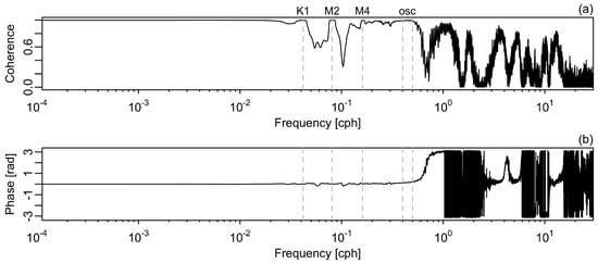
Figure 6.
Cross-spectral analysis of sea level at tide gauges #490 and #491. (a) Coherence, with an indication of the frequencies of three tidal constituents and the h to h band labelled “osc”. (b) Phase difference between signals recorded at the two tide gauges, with positive values indicating that signals appear at #490 before they appear at #491.
The temporal variation in oscillation frequency and intensity was studied by breaking the sea level observations down into daily subintervals and then computing spectra for each subinterval. Figure 7 shows the results. As in Figure 4, the southerly tide gauge, #490, displays less energy in the h to h band than is the case for the northerly gauge, #491. It is difficult to discern seasonal variations in frequency, but there is some indication of such variation in amplitude, with higher values tending to be seen in the winter months.
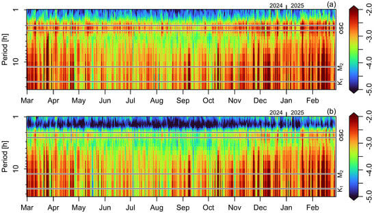
Figure 7.
Temporal variation in power spectra of de-tided sea level records at tide gauges #491 and #490, in panels (a,b), respectively. The spectra are computed daily from the 1 min data, with only periods in excess of 1 h being shown here. Colour indicates the base-10 logarithm of spectral density, in . The and periods (ill-resolved for daily windows) are indicated with horizontal lines, along with the oscillation band from the to h period.
ACF analysis of data at the tide gauge #491, shown in Figure 8, sometimes indicated peaks in the 5 h to 6 h band, perhaps reflecting atmospheric effects. Trimming periods in excess of 4 h, we may compute an observed period of h, where the uncertainty is taken as the standard deviation.
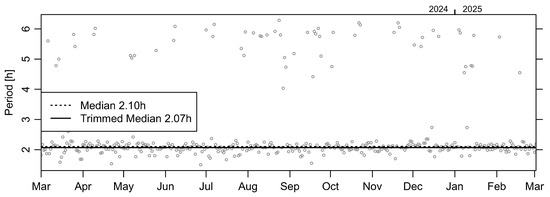
Figure 8.
Daily estimates of sea level oscillation period at tide gauge #491, computed as the lag time of the first peak of the ACF (skipping the zero lag point) for the difference between the observed signal and a cubic spline with 4 knots per period. The horizontal lines show the median computed for all 365 points and a trimmed median computed using only periods of 4 h or less. Note that the median and trimmed median agree to 2 significant digits.
Visual inspection of Figure 8 suggests that the oscillation period does not change appreciably through the year. To check this, the data (again, with oscillation period h) were subjected to least-squares regression using a model assuming sinusoidal variation with a 1 y period. The resultant p value of greatly exceeds the commonly used threshold of , indicating a lack of statistical significance. Furthermore, the adjusted value reveals that only % of the signal variance is explained by this model of seasonal variation in oscillation period.
With this indication that the oscillation frequency is constant throughout the year, a complex demodulation analysis was performed to explore whether its amplitude varies with season and the spring-neap cycle of the tides (Figure 9). As with the spectral analysis, there is some evidence of enhancement in the winter months, but the pattern is not strong or consistent. There is even less evidence of a connection with the spring-neap tidal cycle. At this point, it may be best to classify the events as episodic, i.e., not displaying a clear pattern of repetition, responding to forcing effects that are not yet determined.
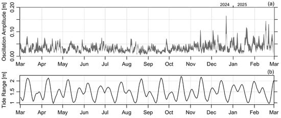
Figure 9.
(a) Complex demodulation amplitude for tide gauge #491, computed in daily subsets. The filled region extends from the median value to that of the 95-th percentile. The prominent spike in December 2024 is for the event shown in Figure 2. (b) Tidal range, again computed in daily subsets, as an indication of the spring-neap cycle.
To explore the practical importance of the oscillations, we computed the ratio of the year-long root-mean-square oscillation amplitude to the same measure for the de-tided amplitude. The result is 18% for the median trace in Figure 9 and 32% for the 95-th percentile trace.
3.2. Theory
3.2.1. Seiche Resonance
Figure 10 shows the prediction of the seiche oscillation period using Equation (1) for Bedford Basin, for a larger domain comprising the basin together with the harbour, for the Northwest Arm, and for Sydney Harbour (311 km northeast of Halifax). The values of H and L were determined by inspection of published charts and should be considered approximations to within perhaps 15%. In the Northwest Arm and Sydney Harbour cases, the observed oscillation periods are consistent with seiche predictions (see [41,42], respectively, for prior work). The same cannot be said for Halifax Harbour, however, since reasonable adjustments to H and L cannot yield a 2 h period.
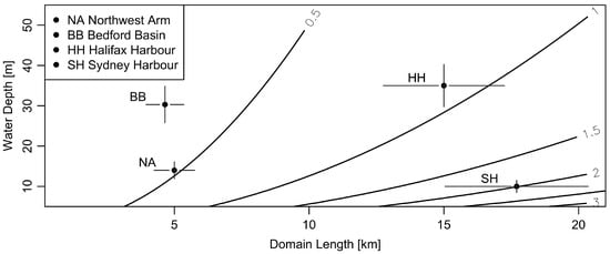
Figure 10.
Dependence of seiche period on domain length and water depth. Contours represent oscillation periods in hours. Points represent 3 subdomains of Halifax Harbour (the Northwest Arm, Bedford Basin, and Halifax Harbour from the northern tip of Bedford Basin to somewhat south of McNabs Island) along with an estimate for Sydney Harbour. The bars indicate an assumed uncertainty of % for each coordinate.
3.2.2. Helmholtz Resonance
The nominal parameter values listed in Table 1 yield and . Since , the system is predicted to be in an oscillatory regime, with the period h in the frictionless limit.
According to Equation (9), frictional damping will change the resonant frequency from to . This yields the theoretical period h. An uncertainty on this value may be inferred with the propagate R package, after assuming a nominal uncertainty of, say, 10% for values not listed with an uncertainty in Table 1. The result, restricting the number of reported digits that reflect the uncertainty, is a theoretical prediction of the oscillation period as h ± h. It is worth noting that this theoretical prediction overlaps with the observed range, h, reported in Section 3.1.
Sensitivity analysis with respect to increasing a, l, A, , U, and h individually from their nominal values to the high end of the stated uncertainty range yields period changes of h, h, h, h, h, and h, respectively. Note that a and l have opposing effects, each being about double the effect of A. All three of these are noticeably larger than the effects relative to , U, and h, which is as expected for this low-friction situation.
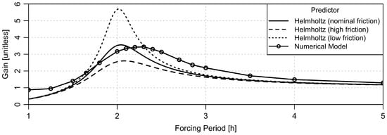
While the sensitivity analysis above indicates that the likely range of drag coefficients is insufficient to significantly modify the location of the peak in the gain function, friction may have a significant effect on the height and width of that peak. This can be seen in Figure 11, which shows the gain that results from using Equation (10) with the values of and stated above, along with the gain that results from altering the friction parameter r in accordance with the confidence intervals for and listed in Table 1. Notice that the location of the peak does not shift visibly for these cases, but that the height and breadth of the response curves vary noticeably across the chosen range of friction parameters.
3.3. Two-Dimensional Numerical Model with Realistic Bathymetry
To discover more details about the possible spatial pattern of oscillations in the domain, the model was run at the resonance period, with results saved at each grid point over two cycles. Then the standard deviation of elevation (over time) was computed at each grid point. This results in a spatial map of the response (Figure 12) that can provide a test of two of the main assumptions behind the Helmholtz theory. The first assumption is that sea level, , can be taken as a constant across Bedford Basin. The GETM simulations suggest that this is indeed the case, at least approximately. The second assumption is that sea level varies linearly along the channel axis, up until a point (at a distance we denote as l) where the variation drops off. This, too, is at least approximately consistent with the pattern shown in Figure 12.
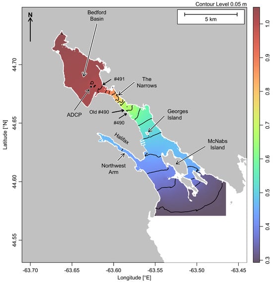
Figure 12.
Spatial pattern of response in the GETM simulations. Colours and contours indicate the standard deviation of simulated sea level, in metres, computed across two oscillation cycles. The contour interval is m. White regions are outside the model domain. Place names are as in Figure 1, except that the bridges are omitted for clarity. As noted in the text, the computational grid covers the narrowest portion of The Narrows with 10 cells.
Returning to the gain function shown in Figure 11, we may assess the agreement between the GETM predictions of oscillation period and the Helmholtz predictions, in the context of the data. There is a visible difference between the GETM resonant period, h, and the Helmholtz period with the base value of the relevant parameters. However, when uncertainties are taken into account, the Helmholtz prediction is h ± h. The two models thus agree reasonably well. Furthermore, both agree with the observed range of h.
4. Discussion and Conclusions
We have shown that Halifax Harbour sea level and current speed are subject to oscillations with a period between h and h, perhaps best characterized as h. The oscillations are intermittent, taking the form of a few cycles, then a quiet period, and then a few more cycles. The typical day has one or more such events. The oscillations represent a significant fraction of the non-tidal variation in sea level, ranging from a median of 18% to a 90-th percentile of 32%. The events appear to be episodic, forced by mechanisms that are yet to be determined. The oscillation strength has been shown to vary throughout the year, although the pattern is not especially clear, so it does not appear that simple wind speed is the key factor. However, wind direction shifts might play a role, perhaps in combination with tides, as has been proposed for the stratified intrusions that are occasionally seen in this system (see, e.g., ref. [43] for a recent treatment of the dynamics and, e.g., ref. [44] for comments on the importance of intrusions to Bedford Basin biogeochemistry). There is little indication that the oscillation events are tied directly to a certain phase of the spring-neap cycle, which argues against tidal currents being the sole forcing agency. However, it may be worth investigating whether the oscillations are triggered by some combination of tidal and other effects. Indeed, a number of possible effects have been explored in the literature on harbour oscillations (see [45,46] for an introduction to the early literature and an application to a series of small harbours). Infragravity waves are a suspected energy source for oscillations with periods in the range of minutes (again, ref. [46] provides a good example). At periods of half an hour and longer, there are a variety of suspected energy sources. For example, a study of oscillations in waters off the Shetland Islands postulated an energy source involving shelf edge waves, possibly driven by rapidly moving meteorological fronts [47]. In another application, ref. [48] investigated the case of high-amplitude internal waves that may be formed hundreds of kilometers from shore, at a location in which tidal currents cross certain topographic features. Combinations between these and other effects (both local and non-local) are also possible, adding to the complexity of the general topic of harbour oscillations.
In the present context, it is worth noting that the oscillations tend to be highly coherent between the two tide gauges in the domain, which suggests that this is a harbour-scale response. The observed oscillation period ( h) is not consistent with seiche theory, but it is in good agreement with Helmholtz resonator theory ( h ± h) as well as with a 2D numerical model that handles realistic bathymetry and computes bottom stress using the law of the wall ( h). The gain function of the Helmholtz theory tends to be somewhat more peaked than that of the numerical simulation, which is perhaps unsurprising, given the detuning that is likely to result from flow in the complex domain in the latter case.
Overall, the reasonable agreement of the frequency response predicted by the Helmholtz theory and the 2D numerical model suggests that it might be possible to calibrate the parameters of the theory to develop a highly efficient tool for short-period predictions of the oscillations in sea level and current. To make progress along these lines, it would be wise to make new measurements of sea level and currents in the domain. Beyond simple calibration of the parameters used here, it might also be worthwhile to extend the Helmholtz model in simple ways, e.g., subdividing the channel to try to capture some effects of realistic bathymetry. Another simple addition would be to add sidewall friction, which was omitted in the present Helmholtz model for simplicity.
But whether follow-up efforts are directed towards enhancing simple theoretical models or calibrating numerical models to the domain, one thing is clear: there is a need for a deeper understanding of the forcing mechanisms that drive the oscillations. A good first step will be to determine whether the forcing is local to the harbour or a nearby region, or whether it extends significantly onto the Scotian Shelf beyond the harbour, or whether it extends even further afield. In the latter case, the modelling effort will be much greater than that employed in the present study, and there will be a need to set up monitoring of sea level and other oceanic and atmospheric characteristics well beyond the harbour.
Author Contributions
Conceptualization, D.K., C.R. and A.H.; methodology, D.K., C.R., R.Y. and A.H.; software, D.K., C.R., K.K. and R.Y.; validation, D.K. and C.R.; formal analysis, D.K., C.R. and A.H.; data curation, D.K. and P.M.; writing—original draft preparation, D.K.; writing—review and editing, C.R., R.Y., A.H., K.K. and R.M.; visualization, D.K. and C.R. All authors have read and agreed to the published version of the manuscript.
Funding
R.Y. was supported by a Natural Sciences and Engineering Research council PGS-D scholarship and a Mitacs Globalink research award that supported travel between Dalhousie University and The Leibniz Institute for Baltic Sea Research Warnemünde.
Data Availability Statement
The raw data supporting the conclusions of this article will be made available by the authors on request.
Acknowledgments
We thank Blair Greenan and Li Zhai of Fisheries and Oceans Canada for their work in establishing tide gauge #490 and assessing the quality of its measurements. We also thank David Greenberg, retired from the same agency, for fruitful discussions relating to this paper and for his provision of the WebTide coefficients used to compute background currents. This paper was written for a Special Issue of this journal dedicated to the memory of our late colleague, Keith R. Thompson. Keith’s early work related to sea level—his PhD dataset comprised a single box of punched cards with measurements of sea level—and he might have been interested in what we have conducted here. We have no doubt that his insights would have surpassed ours. We miss him, not just for his intellect, but also for his boundless generosity and his quick humour.
Conflicts of Interest
The authors declare no conflicts of interest.
Abbreviations
The following abbreviations are used in this manuscript:
| ACF | Autocorrelation function |
| ADCP | Acoustic Doppler current profiler |
| CHS | Canadian Hydrographic Service |
| DFO | Department of Fisheries and Oceans (Canada) |
| GETM | General estuarine transport model |
| NONNA | Non-navigational bathymetric data |
| RMS | Root-mean-squared |
References
- Port of Halifax. Statistics, 2023. Available online: https://www.porthalifax.ca/wp-content/uploads/2024/05/Trade-Statistics-2023-One-Page-Summary-for-Website.pdf (accessed on 23 May 2025).
- McCanne, L.D. Halifax. The Canadian Encyclopedia. 2023. Available online: https://www.thecanadianencyclopedia.ca/en/article/halifax (accessed on 23 May 2025).
- Fader, G.B.J.; Buckley, D.E. Environmental geology of Halifax Harbour, Nova Scotia. Geosci. Can. 1996, 22, 152–171. [Google Scholar]
- Raddal, T.H.; Kimber, S. Halifax, Warden of the North; Nimbus Publishing: Halifax, NS, Canada, 2010. [Google Scholar]
- Dawson, W.B. Survey of Tides and Currents in Canadian Water: Report of Progress 1899; Technical report; Government Printing Bureau: Ottawa, ON, Canada, 1900. Available online: https://waves-vagues.dfo-mpo.gc.ca/library-bibliotheque/41057909.pdf (accessed on 23 May 2025).
- Dawson, W.B. Variation in the leading features of the tide in different regions. J. R. Astron. Soc. Can. 1907, 1, 213. [Google Scholar]
- Ihaka, R.; Gentleman, R. R: A language for data analysis and graphics. J. Comput. Graph. Stat. 1996, 5, 299–314. [Google Scholar] [CrossRef]
- R Core Team. R: A Language and Environment for Statistical Computing; R Foundation for Statistical Computing: Vienna, Austria, 2025. [Google Scholar]
- Kelley, D.E. Oceanographic Analysis with R; Springer: New York, NY, USA, 2018. [Google Scholar]
- CRAN. The Comprehensive R Archive Network, 2025. Available online: https://cran.r-project.org/ (accessed on 23 May 2025).
- Canadian Hydrographic Service. NONNA—Service Hydrographique du Canada, 2025. Available online: https://data.chs-shc.ca/dashboard/map (accessed on 23 May 2025).
- Kelley, D.; Richards, C.; Layton, C. oce: Analysis of Oceanographic Data, 2024. R Package Version 1.8.4. Available online: https://CRAN.R-project.org/package=oce (accessed on 23 May 2025).
- Department of Fisheries and Oceans. Marine Environmental Data Section Archive, 2025. Available online: https://meds-sdmm.dfo-mpo.gc.ca (accessed on 23 May 2025).
- Kelley, D.; Howard, A.; Harbin, J. dod: Download Oceanographic Data, 2025. R Package Version 0.1.16. Available online: https://github.com/dankelley/dod/ (accessed on 23 May 2025).
- Shumway, R.H.; Stoffer, D.S. Time Series Analysis and its Applications: With R Examples, 4th ed.; Springer: New York, NY, USA, 2016. [Google Scholar]
- Stoffer, D. astsa: Applied Statistical Time Series Analysis, 2012. R Package Version 2.2. Available online: https://CRAN.R-project.org/package=astsa (accessed on 23 May 2025).
- Soetaert, K.; Hindmarsh, A.C.; Eisenstat, S.C.; Moler, C.; Dongarra, J.; Saad, Y. rootSolve: Nonlinear Root Finding, Equilibrium and Steady-State Analysis of Ordinary Differential Equations, 2023. R Package 1.6. Available online: https://CRAN.R-project.org/package=rootSolve (accessed on 23 May 2025).
- Cilders, D.G.; Pau, M.T. Complex demodulation for transient wavelet detection and extraction. IEEE Trans. Audio Electroacoust. 1972, AU-20, 295–308. [Google Scholar] [CrossRef]
- Ligges, U.; Short, T.S.; Kienzle, P.K.; Schnackenberg, S.; Billinghurst, D.; Borchers, H.W.; Carezia, A.; Dupuis, P.; Eaton, J.W.; Farhi, E.; et al. Signal: Signal Processing, 2024. R Package Version 1.8.1. Available online: https://CRAN.R-project.org/package=signal (accessed on 23 May 2025).
- Hourston, H.G.; Wan, D.; Guan, L. New Tools for ADCP Data Processing; Technical Report 336; Institute of Ocean Sciences: Sidney, BC, Canada, 2021. [Google Scholar]
- Spiess, A.N. Propagate: Propagation of Uncertainty, 2025. R Package Version 1.0-7. Available online: https://CRAN.R-project.org/package=propagate (accessed on 23 May 2025).
- Taylor, B.N.; Kuyatt, C.E. Guidelines for Evaluating and Expressing the Uncertainty of NIST Measurement Results; NIST Technical Note 1297; U.S. Department of Commerce Technology Administration: National Institute of Standards and Technology: Gaithersburg, MD, USA, 1994.
- Darwin, G.H. The Tides and Kindred Phenomena in the Solar System; Houghton, Mifflin and Company: Boston, MA, USA; New York, NY, USA, 1899; Available online: https://www.gutenberg.org/files/38722/38722-pdf.pdf (accessed on 23 May 2025).
- Gill, A.E. Atmosphere-Ocean Dynamics; Academic Press: New York, NY, USA, 1982. [Google Scholar]
- Green, G. On the motion of waves in a variable canal of small depth and width. Trans. Camb. Philos. Soc. 1837, 6, 457–462. [Google Scholar]
- Helmholtz, H.L.F. On the Sensations of Tone, 4th ed.; Longmans, Green, and Company: London, UK, 1912. [Google Scholar]
- Mullarney, J.C.; Hay, A.E.; Bowen, A.J. Resonant modulation of the flow in a tidal channel. J. Geophys. Res. Ocean. 2008, 113, 2007JC004522. [Google Scholar] [CrossRef]
- Bowden, K.F. Note on wind drift in a channel in the presence of tidal currents. Proc. R. Soc. London. Ser. Math. Phys. Sci. 1953, 219, 426–446. [Google Scholar]
- Rooth, C. A linearized bottom friction law for large-scale oceanic motions. J. Phys. Oceanogr. 1972, 2, 509–510. [Google Scholar] [CrossRef][Green Version]
- Hunter, J. A note on quadratic friction in the presence of tides. Estuar. Coast. Mar. Sci. 1975, 3, 473–475. [Google Scholar] [CrossRef]
- Wright, D.G.; Thompson, K.R. Time-averaged forms of the nonlinear stress law. J. Phys. Oceanogr. 1983, 13, 341–345. [Google Scholar] [CrossRef][Green Version]
- Symon, K.R. Mechanics, 3rd ed.; Addison-Wesley World Student Series; Addison-Wesley: Boston, MA, USA, 1980. [Google Scholar]
- McMillan, J. Turbulence Measurements in a High Reynolds Number Tidal Channel. Ph.D. Thesis, Dalhousie University, Halifax, NS, Canada, 2017. [Google Scholar]
- Fan, R.; Zhao, L.; Lu, Y.; Nie, H.; Wei, H. Impacts of currents and waves on bottom drag coefficient in the East China Shelf Seas. J. Geophys. Res. Ocean. 2019, 124, 7344–7354. [Google Scholar] [CrossRef]
- McGonigal, D.; Loucks, R.; Ingraham, D. Halifax Narrows: Sample Current Meter Data 1970–1971; Data Series BI-D-74-5; Bedford Institute of Oceanography: Dartmouth, NS, Canada, 1974. [Google Scholar]
- Dupont, F.; Hannah, C.; Greenberg, D.; Cherniawsky, J.; Naimie, C. Modelling system for tides. Can. Tech. Rep. Hydrogr. Ocean. Sci. 2002, 221, vii+72pp. Available online: https://www.bio.gc.ca/science/research-recherche/ocean/webtide/documents/WebTide_report4.pdf (accessed on 23 May 2025).
- Department of Fisheries and Oceans. WebTide Tidal Prediction Model, 2023. Available online: https://www.bio.gc.ca/science/research-recherche/ocean/webtide/index-en.php (accessed on 23 May 2025).
- Saltelli, A.; Tarantola, S.; Campolongo, F. Sensitivity analysis as an ingredient of modeling. Stat. Sci. 2000, 15, 377–395. [Google Scholar]
- Burchard, H.; Bolding, K. GETM, A General Estuarine Transport Model: Scientific Documentation; Technical report; European Commission: Brussels, Belgium, 2002; Available online: https://publications.jrc.ec.europa.eu/repository/handle/JRC23237 (accessed on 23 May 2025).
- GETM developers. A 3D Hydrodynamic Model for Coastal Oceans, 2025. Available online: https://getm.eu/bdys.html (accessed on 23 May 2025).
- Stucchi, D.J. Seiches in the Northwest Arm of Halifax Harbour. Master’s Thesis, Dalhousie University, Halifax, NS, Canada, 1975. [Google Scholar]
- Petrie, B. Sydney Harbour: Seiches, tides and mean circulation. Proc. Nova Scotian Inst. Sci. (NSIS) 2022, 52, 225. [Google Scholar] [CrossRef]
- Sui, Y.; Sheng, J.; Lu, Y.; Chen, S. Intense lateral intrusion of offshore sub-surface waters in Halifax Harbour. Cont. Shelf Res. 2024, 277, 105245. [Google Scholar] [CrossRef]
- Rakshit, S.; Dale, A.W.; Wallace, D.W.; Algar, C.K. Sources and sinks of bottom water oxygen in a seasonally hypoxic fjord. Front. Mar. Sci. 2023, 10, 1148091. [Google Scholar] [CrossRef]
- Okihiro, M.; Guza, R.T.; Seymour, R.J. Excitation of seiche observed in a small harbor. J. Geophys. Res. Ocean. 1993, 98, 18201–18211. [Google Scholar] [CrossRef]
- Okihiro, M.; Guza, R.T. Observations of Seiche Forcing and Amplification in Three Small Harbors. J. Waterw. Port, Coastal, Ocean. Eng. 1996, 122, 232–238. [Google Scholar] [CrossRef]
- Cartwright, D.E.; Young, C.M. Seiches and tidal ringing in the sea near Shetland. Proc. R. Soc. London. Math. Phys. Sci. 1974, 338, 111–128. [Google Scholar]
- Chapman, D.C.; Giese, G.S. A Model for the generation of coastal seiches by deep-sea internal waves. J. Phys. Oceanogr. 1990, 20, 1459–1467. [Google Scholar] [CrossRef]
Disclaimer/Publisher’s Note: The statements, opinions and data contained in all publications are solely those of the individual author(s) and contributor(s) and not of MDPI and/or the editor(s). MDPI and/or the editor(s) disclaim responsibility for any injury to people or property resulting from any ideas, methods, instructions or products referred to in the content. |
© 2025 by the authors. Licensee MDPI, Basel, Switzerland. This article is an open access article distributed under the terms and conditions of the Creative Commons Attribution (CC BY) license (https://creativecommons.org/licenses/by/4.0/).