Sea Surface Temperature Fronts and North Atlantic Right Whale Sightings in the Western Gulf of St. Lawrence

Abstract

Sea surface temperature (SST) fronts during 2000–2021 are examined in the Western Gulf of St. Lawrence (wGSL), where North Atlantic right whales (NARW, Eubalaena glacialis) have begun to aggregate and feed. During 2017–2020, from May to October, NARW spatial distributions reveal regional, seasonal, and interannual variations in the Shediac Valley and off the Northern Gaspé Peninsula, and preferentially in waters with relatively strong temperature gradients. Correspondence between SST fronts and NARW sightings is explored using a monthly probability of occurrence, based on an SST gradient threshold and water depths in the range 50–200 m. Spring and summer associations suggest that satellite-derived SST gradients may aid in short-timescale NARW monitoring by way of providing spatial distribution maps of the regional probability of occurrence.

1. Introduction

The North Atlantic right whale (NARW, Eubalaena glacialis) is a critically endangered species; the geographic areas of its foraging habitat have been routinely revisited by satellite remote sensing for decades. Since 2015, NARW sightings have become more frequent in the Gulf of St. Lawrence (GSL), where the whales prey on the zooplankton Calanus spp. [1,2]. In an effort to avoid injury by ship strikes or entanglement in fishing gear, we need to monitor NARW presence and aggregations of their prey using existing environmental monitoring measures. Although not designed for this purpose alone, satellite observations of sea surface temperature (SST) are a familiar component of marine ecosystem monitoring. Moreover, they can provide observations that are suitable for the construction of the appropriate composite indices, in part because interannual SST variations can modulate plankton development and thereby provide a linkage between the whales and the food chain (e.g., [3,4,5]). A composite index of NARW presence in the GSL can also be considered at daily or monthly scales, where zooplankton aggregation is expected to depend, in part, on ocean currents [6,7]. Here, we consider another (sub)monthly index contribution, as given by SST observations, which offers a complementary view of zooplankton aggregation.

Ocean fronts are often associated with enhanced biological activity [8,9,10,11,12]. The common definition of an oceanic front is a relatively narrow convergence of two dissimilar water masses, with an enhanced horizontal gradient of water properties (temperature, salinity, nutrients, etc.) [12,13,14,15]. Among the mechanisms that produce fronts in the coastal ocean are geostrophic currents, estuarine buoyancy currents, tidal mixing, river plumes, coastal upwelling, or water mass convergence zones [12,16,17]. Dynamic processes, including thermal fronts, eddies, and upwelling, are associated with convergence through the water column, enhanced primary and secondary production, plankton aggregation, and biological productivity [8,11,12,18,19,20]. These mesoscale processes generally affect spatial scales of 1 to 10 km and temporal scales of 1 to 10 days [21]. Zooplankton movement notwithstanding, highly concentrated prey patches have been observed and modelled in near-surface convergence zones and throughout the water column [2,8,9,10,22]. Phytoplankton and zooplankton aggregations enhance foraging efficiency and attract many fish species and whales [23]. For example, Ryan et al. [20] revealed an association between blue whales and wind-driven coastal upwelling, which was followed by rapid prey aggregation in the Central California Current.

Oceanic fronts are often considered a proxy for the surface aggregation of Calanus spp. and associated marine mammal predators (e.g., [24,25,26]). Hamazaki [27] demonstrated a correlation between rorqual abundance and areas characterized by a higher monthly probability of ocean front occurrences in the Mid-Western North Atlantic Ocean. Baumgartner et al. [28] investigated NARW presence and physical and biological associations over a 3-year period and suggested that interannual variations in NARW presence in the Roseway Basin are associated with SST gradients, with fronts and eddies, which promote prey aggregation. Similarly, in the Northern GSL, Doniol-Valcroze et al. [26] found SST fronts to be correlated with the distribution of four species of rorqual whales.

Frontal features may be a proxy of NARW prey or presence and can be expected to complement a baseline composite index (cf. [4,5]), as NARW prey presence can also be modulated by other mechanisms ([2,26,29]). Nevertheless, by capturing mesoscale processes at high spatiotemporal resolution, satellite SST is useful in marine ecology and fisheries research [12,30,31,32], by revealing hot spots of plankton aggregation areas. These are, therefore, of interest for the Bay of Fundy [33], the Mid-Western North Atlantic Ocean [27], the Baja California Peninsula [34], the Scotia Shelf [28], and the Northern GSL [26].

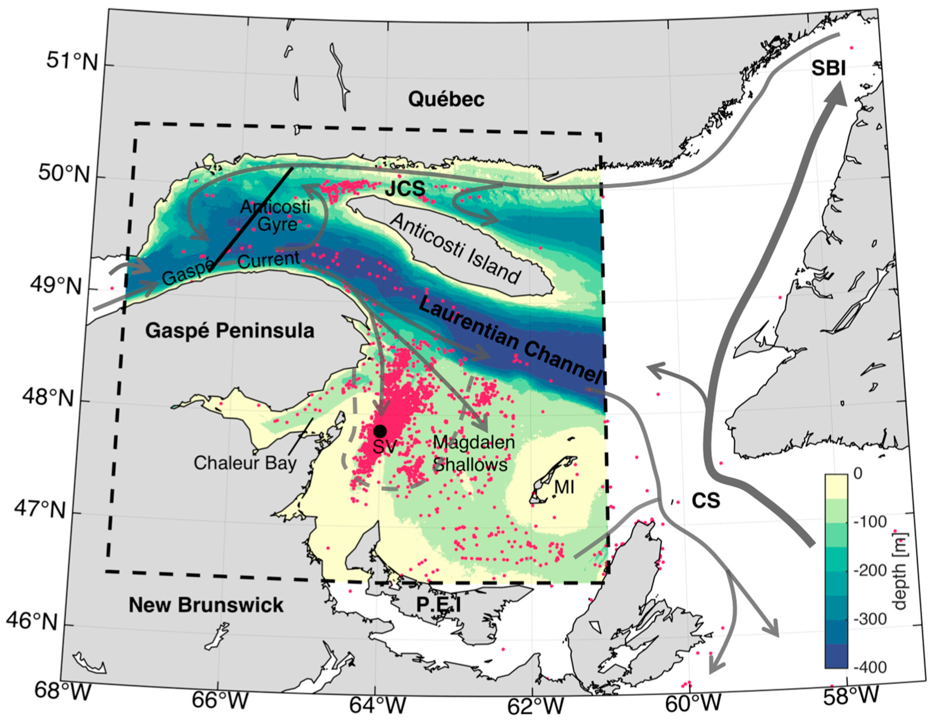
1.1. GSL Circulation

The GSL is a highly stratified semi-enclosed sea that is connected to the Atlantic Ocean and receives considerable freshwater from surrounding rivers, notably from the St. Lawrence River (Figure 1), and salty Atlantic water through the Laurentian Channel, which is over 300 m deep. This system is highly productive, providing support for fisheries along the Canadian Atlantic coast [35]. The Southern GSL (sGSL) is a broad plateau with depths seldom exceeding 80 m [36,37]. The GSL’s circulation is mainly affected by buoyancy forcing and wind-stress forcing. Buoyancy forcing due to freshwater input and surface heat flux demonstrates significant seasonal variability [36,38]. Typically, runoff reaches its maximum level in May, atmospheric heat flux peaks in June, and wind-stress forcing (a crucial source of kinetic energy) peaks in fall and winter, preceding the formation of winter ice cover.

The Gaspé Current (GC) and Anticosti Gyre are significant features of near-surface circulation in the GSL. The GC is a strong coastal current that develops in the St. Lawrence Estuary. It is reinforced by a southward coastal current at the mouth of the Estuary, and generally intensifies around the Gaspé Peninsula [36,39,40]. A segment of the GC recirculates cyclonically within the Northwest GSL and merges with a barotropic westward jet along the north shore of the GSL [36,40], thereby forming the Anticosti Gyre. The main branch of the GC continues eastward along the Gaspé Peninsula, carrying buoyant estuarine waters into the sGSL [38,40]. The magnitude of the freshwater discharge from the St. Lawrence River plays a critical role in controlling stratification and dynamic forcing in the GC. Additionally, robust wind forcing and interactions with other dynamic features, such as the westward jet along the GSL north shore, also affect the behavior of the GC [36,40,41,42]. The GC is characterized by strength and warmth in the summer, and it exhibits weakness and coldness in the winter [38].

The Jacques Cartier Strait is located between the north shore of the GSL and the north side of Anticosti Island (Figure 1), where it receives the freshwater discharged from several rivers. The depth of the Jacques Cartier Strait exceeds 100 m in the mid-channel area, with a maximum depth that is about 250 m. This region is characterized by wind-induced upwelling and strong tidal mixing along the northern shores of the Gulf, which affect local biological processes and fish migration [26,36].

Fronts and mesoscale dynamics are common occurrences in the GSL due to the high buoyancy input from multiple rivers. The highest probabilities of frontal structures in the GSL appear in regions that include the western portion of Jacques Cartier Strait and the mouth of Chaleur Bay [17]. In these areas, fronts are likely formed as a consequence of frequent upwelling caused by the dominant northwestern winds [33]. Another prominent frontal structure that is visible corresponds to the separation between the GC and the Anticosti Gyre [17].

1.2. The North Atlantic Right Whale in the sGSL

In recent years, the GSL has gained recognition as a feeding ground for NARWs from spring to fall [2]. Sightings of NARWs have been abundant in the sGSL, especially in the vicinity of the Shediac Valley (SV), but also in the Jacques Cartier Strait [43]. Passive acoustic monitoring from 2011 onwards has revealed NARWs in the sGSL from the end of April through mid-January, with a peak acoustic presence occurring between August and the end of October [44].

Large-scale variations in whale prey biomass have been examined by Lehoux et al. [45], Gavrilchuk et al. [46], and Blais et al. [47]. The late stages of the copepods Calanus finmarchicus and Calanus hyperboreus are major components of the NARW diet [2,28]. Previous research has indicated that the GC serves as the primary pathway for the transport and aggregation of zooplankton in the Western GSL (wGSL) (Figure 1, black dashed box), likely influencing whale distribution and behavior patterns [22,48,49,50]. The GC provides Calanus spp. from the St. Lawrence Estuary and Northwest GSL. The circulation within the lower St. Lawrence estuary functions as a ‘Calanus pump’, drawing diapausing Calanus finmarchicus copepodites through the deep inflow, and exporting early active stages of Calanus via the surface outflow [51,52]. Southward intrusion of Calanus into the sGSL by the GC along the tip of the Gaspé Peninsula is influenced by runoff and wind conditions [22]. As a physical driver of zooplankton supply, the strength of the GC can be considered a potential predictor of NARW foraging habitat variations.

The relationship between a high prey concentration and a whale’s foraging habitat is indeed complex. NARWs demonstrate an ability to detect patches with high concentrations of prey from a considerable distance and tend to remain within these prey-rich areas while feeding (e.g., [53]). Although high Calanus concentrations are also observed (depth-integrated) elsewhere in the GSL [54], NARWs are frequently observed in the sGSL. This may be explained by the fact that prey aggregations can occur at depths that NARWs cannot readily access without physiological stress and excess energy expenditure, which might occur during deeper foraging dives [55]. Thus, both the depth and the concentration of Calanus aggregations contribute to the suitability of whale foraging habitats.

The goal of this research is to explore an association between SST fronts and visual sightings of NARWs in the wGSL by proposing a composite index for the presence of NARW prey. Moreover, we consider the possible dynamic influences on whale foraging habitat selection through the use of satellite-derived SST gradients at moderate spatiotemporal resolution. We assume that Calanus prey are transported into the sGSL in abundance, and we explore the hypothesis that NARW spatiotemporal distributions can be linked to areas that are associated with strong thermal frontal activity, specifically that whales tend to be found closer to SST fronts rather than being randomly distributed.

2. Materials and Methods

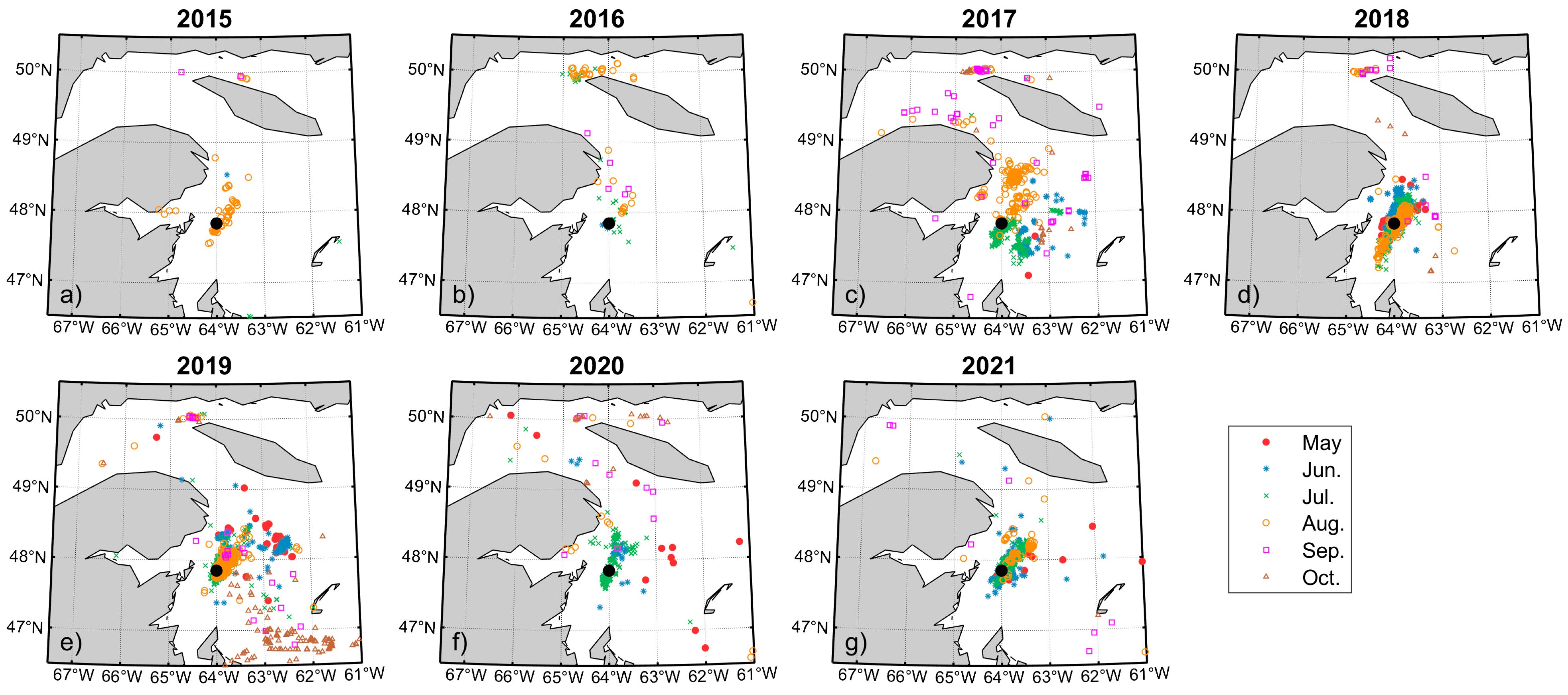
2.1. NARW Sightings

Counts of NARW sightings, based on combined sightings from the North Atlantic Right Whale Consortium [56,57] and Fisheries and Oceans Canada [58] (all non-effort corrected), are listed in

Table 1. Distributions across years and months of whale sighting observations in the wGSL (black dashed box in Figure 1) between 2015 and 2021.

Month Year	May	Jun.	Jul.	Aug.	Sep.	Oct.	All Month
2015	0	4	3	264	2	0	273
2016	0	5	69	70	12	0	156
2017	4	280	828	513	141	45	1811
2018	96	912	1090	725	39	22	2884
2019	52	210	891	685	28	178	2044
2020	13	82	318	17	32	31	493
2021	24	246	564	117	8	1	960
All Year	189	1739	3763	2391	262	277	8621

. Associated spatial distribution patterns from 2015 to 2021 are shown in Figure 2. Fewer sightings are apparent in 2015, 2016, and May to mid-June 2017, with a large increase in encounters starting in the summer of 2017. This rise in sightings can be attributed, at least in part, to the comparatively limited search efforts during the earlier period, as opposed to the heightened search efforts during the latter period, which include systematic cetacean surveys starting in the summer of 2017 [43,59]. NARW sightings have been largely concentrated in the sGSL, in the vicinity of the SV station (black dot in Figure 2), where many search efforts have occurred. There is notable variability in NARW sighting distributions during 2016–2021. Whale sightings were more concentrated around the SV in 2018 and 2021 and more widely scattered to the south and east in 2017 and 2019. In the spring of 2017 and 2019 (May and June), the whales were observed far from the coast, predominantly to the east, in the SV area and along the southern slope of the Laurentian Channel (Figure 2c,e). In October 2019, some NARWs were even spotted between Prince Edward Island and the Magdalen Islands. There were limited NARW sightings to the northwest of Anticosti Island.

It is important to acknowledge that these sighting data may exhibit biases towards specific areas and times when search efforts have occurred and do not capture all NARWs present in all areas or throughout all time periods. An example is the intensive aerial cetacean survey efforts conducted by Fisheries and Oceans Canada (DFO) and the National Oceanic and Atmospheric Administration (NOAA) over this time period [43]. Duplicate sightings may also be present, such as when the same whales are reported by multiple platforms. Therefore, these data should not be directly interpreted as the total number or density of whales across space and time, and the absence of sightings in a specific area or during a certain time should not be interpreted as the absence of whales. There is uncertainty and limitation in understanding the complete distribution and presence of NARWs in the GSL over time, since systematic surveys are primarily conducted in areas where NARWs are expected to aggregate. Therefore, when accessing interannual differences in NARW distributions in the sGSL, it is essential to consider the search effort and survey coverage [43].

Historical whale sightings are encounters between humans and whales. But the lack of an encounter is only an indication of whale absence, human absence, or poor observing conditions (e.g., related to fog or rain), but not necessarily any one of these alone. We define an index of scatter in the position of whale sightings as the mean distance of whale sightings to a fixed position, within one month.

$$Inde{x}_{scatter}=\sum {\displaystyle \frac{position-fixposition}{numberofwhalesightings}}$$

(1)

where, for example, the fixed position is the latitude and longitude of the SV station (47.85° N, −64° W), and whale sightings are observed in the vicinity of the SV station (46.5° N~49° N; −65° W~−62° W). We focus on the Magdalen Shallows (Figure 1, from SV to the Magdalen Islands), which has been shown to be a suitable foraging habitat for NARWs [22,46,54].

Figure 3 reveals the seasonal and annual variation of the scatter index for whale sightings and sighting counts in the vicinity of the SV station during 2015–2021. We ignore the scatter index with small monthly sighting counts (<10; labeled by the shadowed areas in Figure 3). A dramatic increase is found in the number of yearly sightings before and after 2017 (Table 1). In July, the number of sightings generally peaks, and the index of scatter is notably lower (~25 km), which indicates that whale sightings are concentrated around the SV station. If variations in sighting efforts can be ignored, then larger counts and smaller scatter indices suggest a suitable foraging habitat for NARWs. In August, a shift in the NARWs’ foraging habitat is found in 2017, with the scatter index achieving its maximum values.

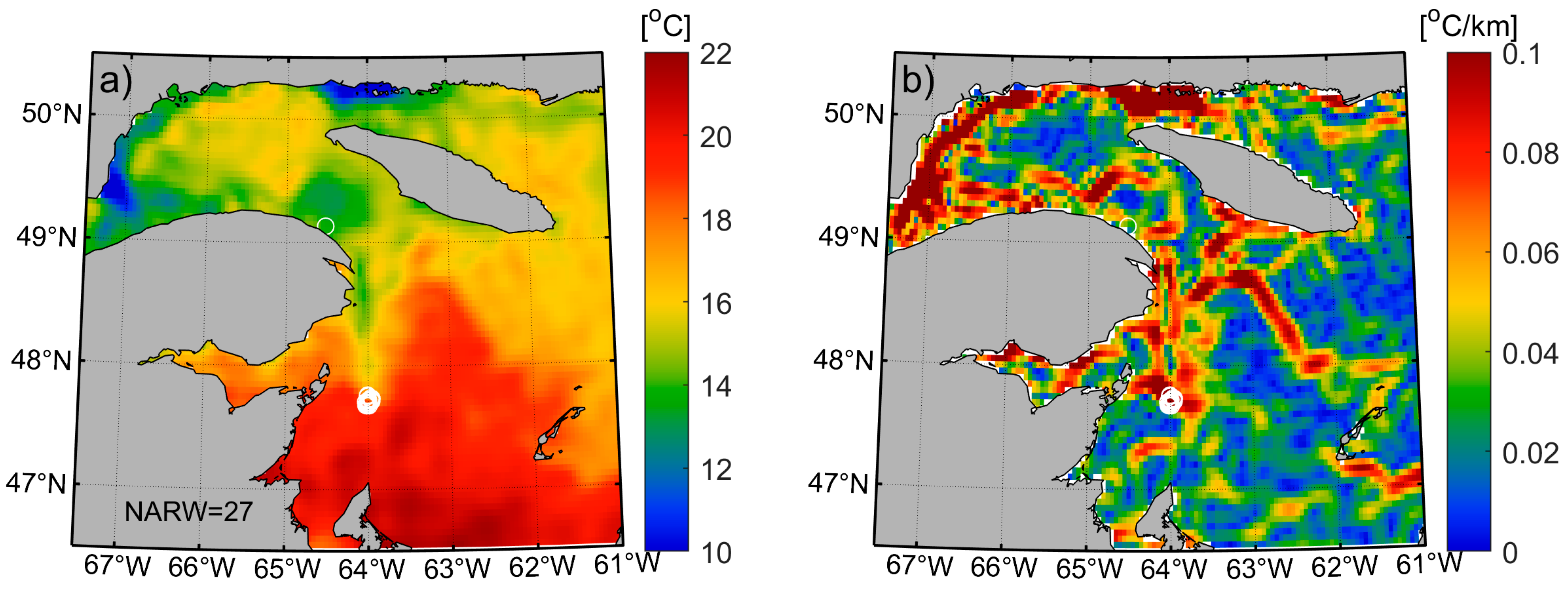
2.2. Satellite SST and Gradients

The Operational Sea Surface Temperature and Sea Ice Analysis (OSTIA) system generates global, daily, gap-filled foundation (without the effects of diurnal warming) SST fields from satellite data and in situ observations [60,61]. The satellite SST data employed in this study were taken from the CMEMS website (Copernicus Marine Environment Monitoring Service, https://marine.copernicus.eu/, accessed on 5 March 2022) for the period 2000–2021. CMEMS OSTIA makes available a reprocessed SST product which is free of diurnal variability on a 0.05° (~6 km) horizontal grid resolution. Because the window from May to October captures the majority of the whale-sighting season, only six months of SST data are used here.

SST gradients are widely used to detect and quantify the frontal regions and their evolution. Daily SST gradients are calculated using the central difference method for each pixel. This is conducted by first calculating the zonal gradient ($G_i$) and meridional gradient ($G_j$) as the ratio of the SST difference among the surrounding pixels. The total SST gradient magnitude ($G$) is computed following other studies (e.g., [31,32]):

$$G_i={\displaystyle \raisebox{1ex}{$[SST\left(i+1,j\right)-SST\left(i-1,j\right)]$}\!\left/ \!\raisebox{-1ex}{$2\times d_i$}\right.}$$

(2)

$$G_j={\displaystyle \raisebox{1ex}{$[SST\left(i,j+1\right)-SST\left(i,j-1\right)]$}\!\left/ \!\raisebox{-1ex}{$2\times d_j$}\right.}$$

(3)

$$G=\sqrt{{G_i}^2+{G_j}^2}$$

(4)

where $i$ and $j$ denote the pixel number in the zonal and meridional directions, respectively. $d_i$ and $d_j$ are the corresponding distances between successive pixels in the zonal and meridional directions, respectively, which are constants here. Daily OSTIA SST data are used to calculate the SST gradients, which are applied to generate bi-monthly and yearly (referred to as May–October) temporal averaging. Bi-monthly SST gradient averages are used to compare with the altimetric index, as described in Section 2.4, and yearly SST gradient averages are used to characterize the interannual variability.

It is valuable to confirm that oceanic fronts and eddies can be identified using SST gradients, as ecosystem (zooplankton) communities have been known to vary with stratification [62]. The SST gradient features are possibly associated with coherent horizontal and vertical circulation processes along which whale prey might accumulate. Thus, frontal structures and eddies may indicate potentially attractive feeding grounds for whales. For example, Figure 4 reveals a group of whales (white open circles) that were sighted at a strong SST gradient near the tip of the GC front. Some oceanic features were also detected using SST gradient patterns, such as fronts near SV and north of the Magdalen shallows, and eddies between the Gaspé Peninsula and Anticosti Island.

The probability density function (PDF, in %) of the distribution of the SST gradient magnitudes for all daily images in years 2000–2021 (green bars) and the distribution of SST gradients corresponding with whale sightings in the years 2015–2021 (purple bars) are shown in Figure 5a for the wGSL. Figure 5b shows the PDF (in %) of the distribution of water depths and the corresponding whale sightings in the wGSL. We identified the SST gradient corresponding with each whale sighting in a 3 × 3 pixel box (~9 km in radius). The whale sightings located in the center of each pixel box and the maximum value of the SST gradient in the pixel box were selected. Considering the spatial lag between oceanic features and whale occurrence, this method is used to identify whether the whale sightings occur in the oceanic frontal zone or not. The mean of all SST gradients is 0.034 °C/km, and the standard deviation is 0.029 °C/km. By comparison, the mean of the SST gradients corresponding to whale sightings is 0.054 °C/km, and the standard deviation is 0.029 °C/km. NARWs mainly occur in the wGSL, where the SST gradient ranges from 0.02 to 0.06 °C/km, which is similar to the observations of Etnoyer et al. [34]. They found that tagged blue whales spent weeks and months in the offshore area of Baja California in areas where the mean SST gradients ranged from 0.022 to 0.05 °C/km.

High values for the SST gradient (above a specified threshold) are used to represent the oceanic fronts. The probability of oceanic front occurrence at each pixel ($Probability(i,j)$) is calculated as a percentage of the number of images with a high gradient exceeding the threshold divided by the total number of available images in a period (e.g., one month):

$$Probability\left(i,j\right)={\displaystyle \frac{HG\left(i,j\right)}{HG\left(i,j\right)+LG\left(i,j\right)}}$$

(5)

where $HG\left(i,j\right)$ and $LG(i,j)$ are the number of images with high gradients and with low gradients, respectively. The total number of available images is, then, just $HG\left(i,j\right)$ plus $LG(i,j)$.

Probability patterns were developed with Equation (5) to characterize the occurrence of oceanic fronts in the wGSL, using satellite SST data from 2000 to 2021. In order to appropriately capture the frontal features in the wGSL, we use a threshold value of 0.035 °C/km to define a SST frontal zone, based on the PDF of SST gradient magnitudes, for all images in this study. Considering the skewed distribution of the SST gradients and the meaningfulness of outliers, we utilize an average gradient value as the threshold. About 70% of the NARWs that were sighted appear mostly in areas where the SST gradients exceed the threshold value. A smaller number of sightings exceeded our cutoff value when we perturbed the sightings, either in space or in time (see Supplementary Material), and sometimes, the mean gradients are significantly smaller (p values < 0.05).

Overall, the threshold values used to define fronts need to vary with respect to the strength of the gradient. For example, the threshold value needed to define fronts is approximately 0.028 °C/km in the mid-latitudes [63], whereas a higher threshold value of 0.1 °C/km is needed in the Inner Sea of Chiloe and its adjacent coastal ocean in Northern Patagonia [31]. By comparison, an intense gradient of 2 °C/km is needed for the Jacques Cartier Strait off the GSL north shore [26].

2.3. Freshwater Discharge and Bathymetry Data

Monthly mean estimates of freshwater discharge at the head of the St. Lawrence Estuary near Quebec City are available from the St. Lawrence Global Observatory (SLGO; https://ogsl.ca/en/freshwater-runoffs-quebec-city-application/, accessed on 1 February 2022). These runoff data are derived using an empirical relationship between the monthly mean discharge and the monthly mean water level at the Neuville tidal gauge [64]. The annual mean freshwater discharge of the St. Lawrence River at Quebec City exhibits a similar variation to the total discharge from all rivers flowing into the Estuary [65]. Figure 6a illustrates the monthly river discharge timeseries for the 2000–2021 period. Typically, the highest monthly mean runoff occurs in April or May. Over the past two decades, the peak runoff, exceeding 20,000 m³/s, was recorded in May of 2011, 2017, and 2019 (Figure 6a). Additionally, most years feature a second, albeit lower, peak river runoff in the late fall, around October. To present the peak runoff of the year and the time taken for it to reach the wGSL, the time series of accumulated river discharge from April to September is shown in Figure 6b. Since 2015, the accumulated runoff during 2017 and 2019 has exceeded 90,000 m³/s, whereas 2021 was one of the lowest runoff years.

Ocean-bottom depth data were obtained from GEBCO 2021 (General Bathymetric Chart of the Oceans; https://www.gebco.net/, accessed on 1 February 2022), which provides gridded elevation data at a 15 arcsec resolution. The bathymetry map covering the wGSL part is shown in Figure 1.

2.4. Altimetric Index of Gaspé Current Intensity

To evaluate the interannual and seasonal variations of GC intensities, we calculated the satellite altimetry-derived sea level anomaly index proposed by Tao et al., [6]. Satellite altimetry provides a measure of the geostrophic surface currents [66,67,68] via the sea surface height slope relative to the geoid. The Jason-2/3 (J2/3) altimeter profiles were employed to calculate an altimetric index of the GC intensity in the GSL [6]. The J2/3 sea level height anomaly (SLA) data were taken from the CMEMS. J2/3 missions follow a repeating ground track (Figure 1) across the GC approximately every 9.9 days. The J2/3 smoothed data, with a 7 km resolution, were collected during May–October from 2015 to 2021. The reanalysis SLA product is employed until June 2020, and the near-real-time product covers the period to October 2021. We calculate the SLA slope along the track (Index_slope-half in cm/km) as a measure of GC intensity, following Perrie et al. [69] and Tao et al. [6]:

$$SLA={\beta }_0+Inde{x}_{slope\text{-}half}·L$$

(6)

where Index_slope-half is a linearly regressed coefficient, ${\beta }_0$ is an additive constant, and $L$ is the distance of the SLA measurements from the intersection of the southern coastline and the ground track. Index_slope-half is calculated using a linear fit of the SLA profile along the southern half of the track (black line in Figure 1; ~49.2° N–~49.7° N). The temporal variations of Index_slope-half will be compared with estimated frontal activity strength (SST gradients) in order to explore the utility of SST gradients on monitoring GC intensity. Due to the limited altimetry measurements in each month, the bi-monthly averages of Index_slope-half and SST gradients are calculated for comparison.

3. Results

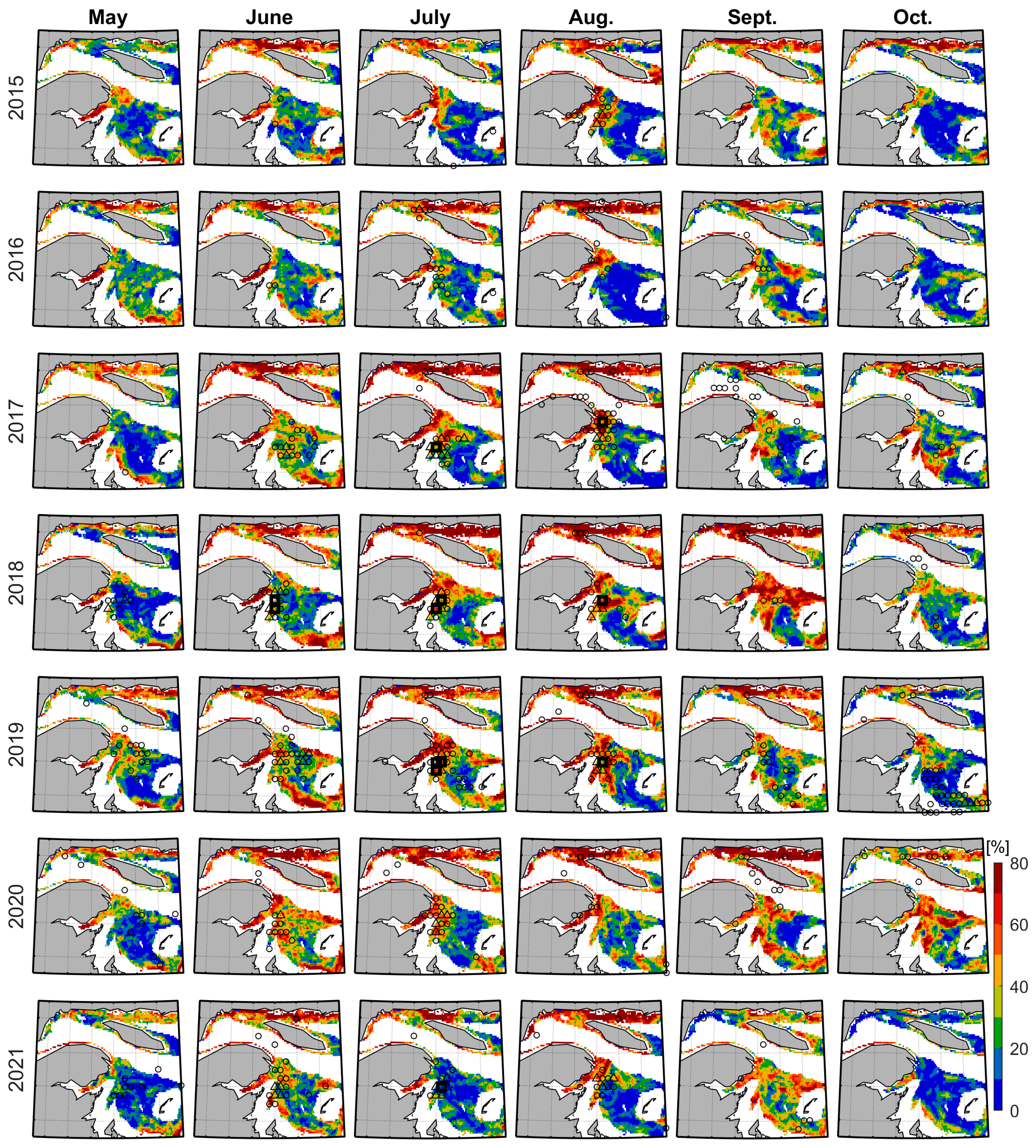
3.1. Variability of Front Occurrence Probability Patterns

Probability distribution patterns provide visualizations to identify regions of persistent oceanic fronts. Figure 7 presents a monthly climatology (2000–2021) of frontal probability from May to October in the wGSL. The seasonal variability in thermal fronts is prominent. SST imagery identifies the high-frequency occurrence of fronts off the north shore of the Gaspé Peninsula, Chaleur Bay, and the Jacques Cartier Strait, where the freshwater is transporting water mass and nutrients into the GSL [17,26,36]. Fronts are found mostly along the coastline in May and then expand to the center of the GSL in September (Figure 7). Lower values for the frontal probability are found in October compared to other months. In general, high probabilities for the frontal zone gradually decrease with distance from the coastline.

Off the north shore of the Gaspé Peninsula, the area with strong probability (>60%) expands from May and reaches a maximum extent in August. Relatively high probability values (strong frontal activity) are observed around the SV area (black box in Figure 7a) from June to August, as well as to the northwest of Anticosti Island from June to September. In contrast to this, the probability values are high in May and June in the Chaleur Bay region, then generally decrease after July. Furthermore, relatively high probability values are seen throughout the Northwest GSL region (north of 49° N). This is possibly caused by strong circulation features, such as the GC, Anticosti Gyre, and wind-generated upwelling [17,36,39,40]. Along the 50–60 m isobath off the Northwestern Prince Edward Island coast, high frontal probability areas are only observed in May and June (Figure 7a,b).

In order to characterize the interannual variability of thermal frontal activity adjacent to the Northern Gaspé Peninsula (NGP) and SV subregions (Figure 7a), the yearly (referred to May–October) mean and standard deviation of the SST gradients have been calculated in each subregion during 2000–2021 using daily data (Figure 8). The mean values of the SST gradients vary around 0.035–0.048 °C/km for the NGP subregion. The time series of SST gradient variability appears to significantly jump during 2000–2004, with low values in 2000 and 2002. Long-term variability appears to have an obvious descending trend in the SST gradients, decreasing approximately 27% from 2004 to 2013. Thereafter, an ascending trend appears, which reaches a peak in 2019 (Figure 8a). The yearly mean of the SST gradients varies around 0.026–0.037 °C/km for the SV subregion, which is lower than that of the NGP subregion. The time series of the variability in SST gradients for the SV subregion displays a similar trend as that of NGP, with several minima in 2000, 2011, and 2021 (Figure 8b). It may be noted that the SST gradients are relatively strong during 2017–2020, during the past decade, for both the NGP and SV subregions.

3.2. Monthly Probability Pattern and Whale Sightings

Frontal features promote the aggregation of prey and enhance the prey availability and are thereby expected to have a significant influence on whale spatial distributions. Since about 70% of NARWs appear mostly in areas with high SST gradients, exceeding the threshold value (0.035 °C/km), and 96% of NARWs appear at depths between 50 m and 200 m (Figure 5), we apply these two simple criteria to estimate probabilities for whale occurrence in the wGSL. Figure 9 displays the monthly frontal probability patterns from May to October during the period 2015–2021, corresponding to NARW sighting distributions. We assume that the prey are relatively abundant and are transported into the sGSL.

In general, prominent interannual and seasonal variability are observed in the high probability patterns. NARWs are observed in the high probability areas during spring and summer (Figure 9). For example, NARWs have been sighted with high frequency off the eastern tip of the Gaspé Peninsula (close to land) in August 2017, which is co-located with high probability areas. In addition, NARWs are generally observed off the northwest coast of Anticosti Island (Jacques Cartier Strait) starting from July, which coincides with increased probability (Figure 7). The area of Jacques Cartier Strait is characterized by persistent wind-driven upwelling during the summer and heavy tidal mixing [26,36]. Whale sightings are normally aggregated around the SV area during July and August, while sightings are scattered away from the SV area during September and October. Within the SV region and off the eastern tip of the Gaspé Peninsula, relatively higher monthly probabilities are observed during July–August compared to May–June. However, disagreements between high probabilities and whale-sighting patterns are also obtained, such as in the fall season and during July 2021 at SV. We note that the probability values are relatively low over the sGSL during July 2021.

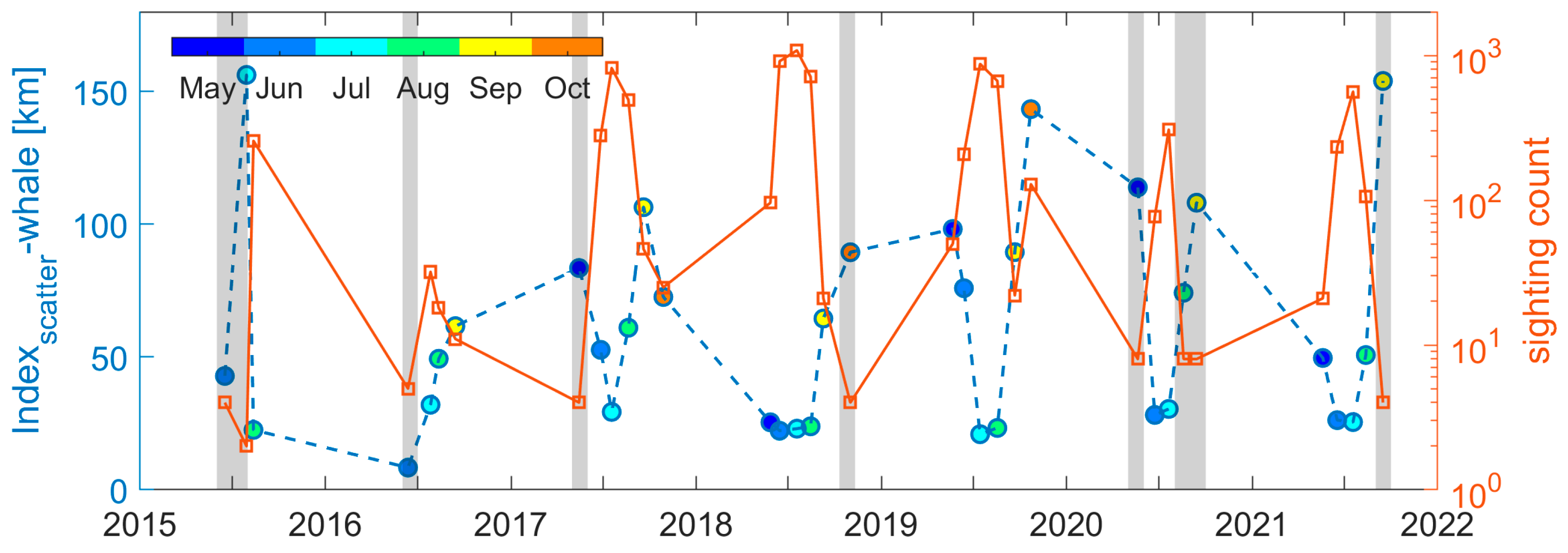
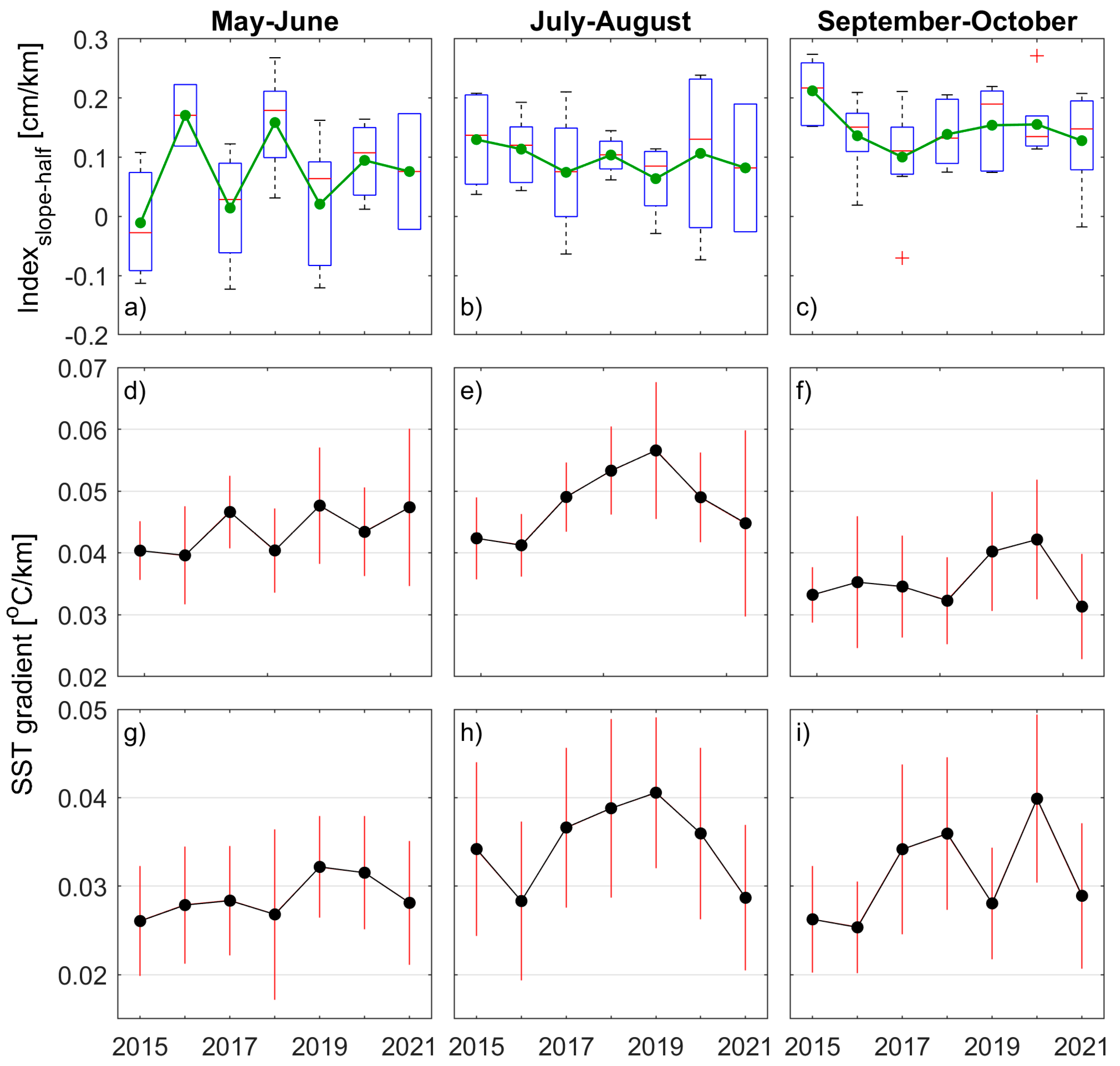
3.3. Variations in the Gaspé Current Indices

The GC is a dominant ocean circulation process in the wGSL, affecting the water mass, nutrients, and prey transport from upstream to the sGSL. Physical indices developed from satellite altimetry data are useful to monitor variations of GC, and specifically, Tao et al. [6] have indicated that Index_slope-half is a proxy for variations in the GC intensity. Index_slope-half values decrease as GC intensity increases. In order to compare the index with whale-sighting distributions, the bi-monthly mean and standard deviation of Index_slope-half are calculated from 2015 to 2021. The temporal variability of Index_slope-half is high, as exhibited in Figure 10a–c. During spring seasons (May and June), the mean values of Index_slope-half show a strong interannual variation, which is much lower in 2017 and 2019 than in 2018 (Figure 10a). The variability of mean Index_slope-half is relatively low during July–August (Figure 10b). However, values of Index_slope-half are slightly larger in September–October, which indicates that the GC strength is weaker (Figure 10c).

Similarly, Figure 10d–i characterize the interannual and seasonal variability of frontal activity strength within the NGP and SV subregions. The bi-monthly mean and standard deviation of the SST gradient magnitudes were calculated for the period 2015–2021. The interannual variations and magnitudes of the mean SST gradients are much more pronounced during July–August in both subregions. During May–June, the SST gradient magnitudes suggest a high level of frontal activity in 2017, 2019, and 2021 in the NGP subregion, and in 2019 and 2020 in the SV subregion (Figure 10d,g). In May–June, the frontal activity shows slightly different behaviors in the upstream and downstream regions. During July–August, the SST gradient magnitudes display a similar variation in these two subregions. Peaks in SST gradients were found in 2018 and 2019 (Figure 10e,h). During September–October, a relatively flat variation in SST gradients was found in the NGP subregion, except for small peaks in 2019 and 2020 (Figure 10f). By comparison, the time series of the SST gradients reveal a significant variation in the SV subregion, and the highest frontal activity is found in 2020 (Figure 10i). It is noted that a bi-monthly variation of SST gradients appears to have some similar variations with Index_slope-half but also reveals notable differences (Figure 10).

4. Discussion

4.1. Probability Patterns of Whale Occurrence

Seasonal variability in NARW occurrence in the SV region might be related to the strong regional abundance of oceanic fronts. Oceanic fronts in the SV region probably play a role in whale prey aggregation processes during spring and summer. Our results demonstrate that whale sightings generally aggregate around the SV region during July–August, which is consistent with the fact that relatively greater monthly frontal probabilities are observed at that time and in that location (Figure 9).

Sorochan et al. [2] elucidated the monthly variation in Calanus spp. biomass and stage composition at the SV station using the sampling data over the years 1999–2016. The monthly average dry weight of C. finmarchicus is highest in July–September, and C. hyperboreus reaches its peaks in May–July. The proportion of C. finmarchicus stage CV (lipid-rich diapause phase) abundance increases from June onwards, in the summer, and reaches a maximum in August. In summer (July–August), NARWs can potentially feed on aggregations of their preferred prey (late stages of C. finmarchicus and C. hyperboreus) in the SV region. Physical features, such as oceanic fronts and filaments, promote the horizontal and vertical aggregation of prey and produce greater prey concentrations [10,18]. Several of these physical processes, such as fronts, upwelling/downwelling, and internal waves, control the movement of buoyant particles on the ocean surface and induce vertical transport and the mixing of particles [70]. Cohen et al. [71] also proposed that the physical environment, such as temperature and hydrodynamic processes, in conjunction with the biological properties of lipids, explains periodic high abundances of lipid-rich copepods in surface waters. These factors may explain why whale sightings are co-located with greater probability in these areas during summer. Similarly, NARWs are found in the lower Bay of Fundy and in the waters off Southwestern Scotia Shelf during summer. The large population of C. finmarchicus consists of stage CV in the water column, which can feed the NARWs there [72,73,74,75,76]. Moreover, Baumgartner et al. [28] also proposed that the occurrence of NARWs on the Southwestern Scotian Shelf, both spatially and interannually, may be correlated with SST gradients.

NARWs have also been frequently sighted in the wGSL, in the vicinity of the Chaleur Trough and SV (Figure 1), which are strongly affected by the ocean circulation, such as, for example, the GC intrusion from the north and outflow from Chaleur Bay. It has been shown that the arrival of the GC contributes to the formation of a front, which in turn, exerts a strong influence on the biological characteristics of this area [77]. Baumgartner et al. [78] suggested that right whales may have the ability to restrict their search for optimal prey concentrations using cues from the surrounding physical environment, such as turbulence within the mixed layer, or rapid velocity changes with depth, or particular temperature or salinity properties. They found a strong correlation between whale dive depths and the depth of maximum C. finmarchicus CV abundance. The depth of maximum Calanus spp. biomass densities is around 50 m in the early summer in the shallow sGSL [46]. This indicates that right whales may have skill in locating and exploiting discrete layers of highly concentrated prey. Maps et al. [79] also show that the Western sGSL is a zone with potential for the formation of dense zooplankton aggregation in summer, based on acoustic observations of krill and also on hydrodynamics model simulations. Their findings are consistent with our observations that the associated oceanic features are prominent in this area (Figure 7 and Figure 9).

The monthly probability patterns reported here demonstrate a noteworthy interannual variability in frontal activities in the sGSL (Figure 9), which is helpful for understanding the distributions of NARWs sightings. For example, although NARWs have been typically observed around the SV station in August, they have also been observed mostly off the eastern tip of the Gaspé Peninsula (close to the land and further north of the SV) in August 2017 (Figure 9). This phenomenon may be partially explained by the high probability area (enhanced frontal activity) near the eastern tip of the Gaspé Peninsula. Comparing monthly probability patterns in August 2017 and 2018, a prominent high probability area is found near the SV in August 2018. Meanwhile, in August 2017, a low probability area was found near the SV, and a high probability area was found near the eastern tip of the Gaspé Peninsula.

However, disagreements between high frontal probability and whale-sighting patterns are also observed (Figure 9). Some areas with higher monthly probability but with fewer NARW sightings and occurrences are found (e.g., September and October). One possible explanation is that changes in whale behavior may contribute to the breakdown in the association between right whale occurrences and ocean fronts in the fall. Franklin et al., [80] observed a potential transition of whale behavior from primarily foraging to increased socializing behavior, based on whale-calling behavior. Other studies also reported that the observations of the gunshot sound produced by male NARWs, potentially functioning as a reproductive advertisement, were lowest in May and June and progressively increased to a maximum in the fall [81,82]. The locations of increased frequency of fronts can be a proxy for potential foraging habitat, but perhaps not for socializing grounds. Another speculative explanation is that the association between right whales and ocean fronts only occurs in particular areas and at particular times. Baumgartner et al. [28] indicated that an increased abundance of oceanic fronts was accompanied by higher sighting rates of NARWs in the Roseway Basin using 3 years of data. However, Baumgartner and Mate [29] suggested that there was no evidence for an association between the distribution of tagged right whales and either surface temperature gradients or surface chlorophyll gradients. In addition, another factor is that lower local prey concentrations may occur in those areas and at those times.

We also note that the agreement between frontal probability patterns and whale-sighting distributions is affected by the concentration and availability of diapausing Calanus spp. to NARWs. The application of frontal probability patterns to predict the presence of whale sightings is limited by the vertical and horizontal distributions and abundance of the prey and by the copepodite stages. In other words, the primary foundation of the association between frontal probability with whale presence is that the copepods need to be relatively abundant and that they are advected into the particular area of interest.

The abundance of C. finmarchicus in the sGSL exhibits near-normal anomalies during 2016–2019, and a below-normal anomaly is found in 2015 [47]. Furthermore, whale-sighting data may be a cause for the disagreement. We acknowledge that the sighting data may be biased in terms of ‘effort’, as they are more likely to reflect areas and times when search effects have been conducted. Thus, they may not fully capture all NARWs present in all areas and at all times. Caveats (search effort and survey coverage) related to these sightings should be considered, as stated in Section 2.2. In this study, we focus more on the spatial distribution of whale sightings in the wGSL, and the abundance of whale sightings related to a high sampling frequency is not considered. In other words, this study specifically concentrates on the alignment between the locations exhibiting heightened front frequency and the occurrences of whales. Further studies, including the correction of sighting data for search effort (e.g., sightings per unit effort) and the incorporation of models of NARW distributions, may improve our comparisons. Also, NARW tagging studies could provide whale movement patterns and diving behaviors that may better resolve our understanding of their interactions with frontal features.

Previous studies have demonstrated that high densities of zooplankton have been observed and modeled in near-surface convergence zones associated with fronts [8,10]. Nevertheless, establishing relationships between the fronts and whale distributions can be challenging, given the high mobility of whales and the fact that physical features are not always associated with high concentrations of prey [2]. The locations of fronts can vary quickly over a few days. The time and spatial lag among frontal areas, aggregation patches of prey, and whale occurrence should also be considered. There may be a time lag between changes in oceanographic conditions and whale responses [27,83,84]. A finite time interval is required between the formation of oceanographic features, the aggregation of prey species, and then, the attraction of the whales. Therefore, a weak relationship may be expected between instantaneous changes in oceanographic features and whale sightings. Additionally, there may be a spatial lag. The actual aggregation of prey items might be several kilometers away from the fronts detected at the surface, since the fronts are often not following straight lines under the water surface [26]. Accommodating a time delay between SST frontal formation and prey aggregation or the presence of right whales, say, by cross-correlation or time-series analysis, could allow closer associations to be recognized.

Uncertainty in the satellite-derived SST also affects the accuracy of its gradient. The OSTIA SST product uses satellite data from both infrared and microwave radiometers with accompanying uncertainty estimates [60], such as cloud cover, sensor errors, and interpolation techniques. Accurate SSTs estimated from infrared sensors can suffer from cloud cover [61]. While the OSTIA employs advanced algorithms and models to generate gap-free SST data, there may still be biases and errors introduced by clouds or interpolation methods, resulting in spatial and temporal biases in the intensity of the SST gradients. Since the threshold value is calculated as the mean of all SST gradients, any biases in the intensity of gradients may consequently impact the selection of our threshold value. However, we applied a high value SST gradient to define a front and examine the SST fronts’ occurrences over a month, which is a relatively long time scale. As a result, the impact of cloud cover on our results (e.g., monthly frontal probability patterns) is expected to be limited. In addition, accurate retrieval of SST gradients should be considered for detecting fronts. There are several methods to calculate SST gradients, e.g., Sobel, Roberts, Prewitt, the central difference method, and Pavel kernels [85]. According to Ciani et al. [85], the central difference method is only relatively more appropriate for highly processed SST estimates, such as the ‘level 4’, denoted as L4 (gapless, daily), product that we employ. As expected, the central difference method is affected by noise in each pixel estimate. Reduction of noise seems relatively more successful for the raw L2 SST products when using Sobel or Pavel kernels. Aside from the 7–11 point kernels, which are not convenient near enclosing coastlines, we believe the Sobel option or higher-order finite-difference methodologies (i.e., using three points in each direction rather than two) would improve the SST gradient, perhaps more so at daily scales than monthly or seasonal scales. We seek to monitor SST gradients in real time and, thus, require a robust daily estimate, but our results currently emphasize applications at longer timescales. To minimize noise in future applications, we anticipate that a tradeoff between spatial coverage in shallow water and the use of L2 SST datasets will require a more complex numerical definition of the SST gradient.

The selection of spatiotemporal scales can also impact the variety and significance of the predictor variables (e.g., the probability patterns discussed here) associated with whale sightings. Given the time and spatial lags mentioned above, we calculate probability maps over a longer period (monthly) and focus on the high probability areas. Even with those uncertainties, our monthly probability patterns are generally consistent with variations in NARW sighting distributions during 2015–2021 in the wGSL. This indicates that monthly probability patterns are useful to explain the whale-sighting distributions in the wGSL, and this method might be applied in other areas. Overall, remote sensing provides an alternate way to repeatedly monitor changes in the spatial distributions of frontal processes that are important to whale habitats. Probability patterns produced with historical data in this study are useful to capture the important relationships between NARW occurrence and frontal activity on the spatiotemporal scales in the wGSL. Therefore, near-real-time SST-based probability maps may contribute a helpful subindex (cf. [4,5]) as a composite near-real-time prediction of NARW occurrence in GSL.

4.2. Linkage Between Indices and NARWs Foraging Habitat

Our altimetric index seems useful to monitor variations in the GC, which play an important role in the advection and horizontal distribution of Calanus in the sGSL, thereby affecting the NARW foraging habitat in the sGSL [22,48,50]. The GC also seems to shape the distributions of whale sightings away from the SV or in the Western sGSL [22]. Previous studies indicate that Index_slope-half is a proxy for GC intensity, and the Index_slope-half values decrease as the GC intensity increases [6]. Moreover, low values of Index_slope-half (strong GC) seem to shape the distributions of whale sightings away from the SV. The seasonal variation in Index_slope-half (mainly in spring and summer) seems broadly consistent with variations in the index of scatter during 2015–2021 (Figure 3 and Figure 10a–c).

In the spring seasons (May and June), the mean of the Index_slope-half values is notably lower in 2017 and 2019 than in 2018, 2020, and 2021 (Figure 10a), which indicates that the GC is stronger in 2017 and 2019, which were extreme runoff years (Figure 6b). Here, we ignore the scatter index values with small sighting counts. In June, the scatter index values are higher in 2017 and 2019 and lower in 2018, 2020, and 2021, which indicate that whale sightings are more widely scattered away from the SV station in 2017 and 2019 and more concentrated around the SV station in the other three years (Figure 3). During the spring of 2017 and 2019, whales were sighted in southeastern waters, away from the SV station, along the southern slope of the Laurentian Channel (Figure 2). In general, changes in the mean Index_slope-half and the scatter index are relatively small and an opposite trend is apparent between the time series of Index_slope-half and the scatter index during July–August (Figure 10b), whereas the GC strength is weak and the scatter index is relatively high in September–October (Figure 10c).

Accordingly, in fall, the NARW foraging habitat in the sGSL may not be directly associated with GC transport. Both the upstream replenishment and the retention of arctic Calanus spp. are lower in fall than in spring and summer in the sGSL [86]. Plourde et al. [54] indicates that a suitable NARW foraging habitat is potentially distributed over a broad area in the sGSL. It is consistent that Figure 9 reveals that the whale sightings during September–October are mainly observed over the Magdalen shallows, for example, between the SV and the Magdalen Islands, between PEI and the Magdalen Islands, and even in the Laurentian Channel. Right whales target aggregations at depth when Calanus hyperboreus completes its annual active period around May–June, enter diapause, and aggregate at depth, whereas Calanus finmarchicus reproduce later in the year and begin to enter diapause in June–July. A portion of this population may stay active and continue diel-vertical migration into the early fall. It follows that vertical migration and subsurface prey distributions are important determinants of whale habitat (see Supplementary Material). Incorporating vertical oceanographic data, such as thermocline depth, stratification, or modeled prey distribution within the water column, would, thus, provide a more comprehensive overview of habitat suitability.

The frontal activity strength (SST gradient) also appears to have explanatory power on the GC intensity in spring and fall. Therefore, we compare the temporal variations of the SST gradients in the NGP subregions with variations in Index_slope-half to explore the utility of frontal activity strength on monitoring GC intensity. During May–June, the SST gradient magnitude suggests strong frontal activity in 2017 and 2019, more than in 2018. This implies that the GC intensity is relatively high in 2017 and 2019 (Figure 10d), which is consistent with Index_slope-half variations during 2017–2019 (Figure 10a). Both suggest a relatively lower GC intensity in September–October (Figure 10c,f). However, temporal variations in the SST gradients show a much stronger and increased trend in frontal activity in July–August during the years 2016–2019 (Figure 10e), whereas a weaker variation in Index_slope-half is found for the same period (Figure 10b). This stronger variation in SST gradients may contribute to the seasonal variation of heat flux from the atmosphere; the surface heat flux increases throughout the summer [36]. However, further research is needed to fully elucidate this hypothesis.

Prominent interannual variability in SST gradients (yearly frontal activity) is represented in the NGP subregion, which shows a different response to cumulative river discharge (April–September) of the St. Lawrence River (Figure 6 and Figure 8a). For example, the cumulative river discharge is much lower in 2001 and 2003, while high values of SST gradients are found in these years. In contrast, yearly SST gradients and cumulative river discharge have similar variations during 2015–2021. This different response may be explained by the SST gradients, which reflect the combined oceanic circulation features, such as dynamic interactions between surface currents (e.g., GC and Anticosti Gyre), bathymetry, and tide- and wind-induced mixing. The amount of freshwater from the St. Lawrence River significantly influences the dynamic forcing on the GC and the circulation pattern in the Northwest GSL [36,87]. Therefore, SST gradients could capture a combined variation, and they are helpful in monitoring the spatial and temporal variability of the oceanographic fronts in the Northwest GSL.

Moreover, yearly and bi-monthly (May–June) frontal activity exhibited the same variation during 2015–2020, which is consistent with river discharge changes (Figure 6b, Figure 8a and Figure 10d). This result suggests that frontal activity derived from the SST gradients can be potentially used to capture the GC variations in springtime for long-term predictions. Furthermore, an increase from low yearly values in 2015–2016 to high values in 2017–2020 is found in the time series of the SST gradients in both the NGP and SV subregions (Figure 8). Since higher frontal activity may represent an enhanced foraging habitat for the NARW, the high SST gradients in 2017–2020 suggest an improvement in the potential feeding conditions, which is aligned with the documented regime shift in NARW presence in the GSL after 2015 [88].

5. Conclusions

Satellite-derived SST gradient data are used to explore the spatiotemporal variability in the frontal probability patterns and their influence on the aggregation areas of NARW sightings in the wGSL. SST gradient patterns are used to detect ocean surface features, such as oceanic fronts and eddies. The monthly climatology frontal probability patterns are derived using 22 years of SST data, which display a prominent seasonal variability in fronts and help further understand the frontal characteristics in the wGSL. SST imagery is used to identify high-frequency oceanic fronts in waters off the north shore of the Gaspé Peninsula, Chaleur Bay, and Shediac Valley, as well as the Jacques Cartier Strait, where freshwater transports of water mass and nutrients into the GSL are affected by strong ocean circulation. Cyr and Larouche [17] indicated that certain frontal regions may be linked to enhanced primary production and organisms at the upper trophic level. The monthly frontal probability patterns may also be useful in fisheries management. The interannual variability of frontal activity within the Northern Gaspé Peninsula (NGP) and the Shediac Valley (SV) subregions is characterized using yearly means of SST gradient data during 2000–2021. The time series of SST gradients in the two subregions display similar trends over the past two decades, and the SST gradients (as a proxy for frontal activity) are found to be relatively strong during the years 2017–2020.

A number of studies reveal that frontal features can promote the aggregation and availability of prey, which can then attract whales (i.e., [20,26]). This study has developed monthly probability patterns for whale occurrence in the wGSL using two simple criteria: SST gradients over the threshold value 0.035 °C/km and water depths in the range of 50–200 m. We assume that prey are transported into the sGSL in abundance and find that NARWs are generally co-located within the high probability areas during spring and summer in the years 2015–2021.

Further research may improve the performance of the probability maps for inferring NARW occurrence, such as by including critical information on the supply of Calanus spp. to the sGSL, as provided by physical–biological models, or by considering monthly spatial patterns of Calanus spp. provided by zooplankton species distribution models. Such information would also complement other high-resolution satellite sensors, such as synthetic aperture radar, which capture features of the ocean current [7]. As a complement to other satellite-based indices, the probability maps developed in this study are useful to monitor variations in frontal activity and help to predict whale foraging habitat, not just interannually [4,5], but on a range of shorter timescales, from weeks to days, to almost near real time. This approach can also help to develop NARW species distribution models in the GSL. These results are consistent with the hypothesis proposed by Doniol-Valcroze et al. [26] that whales are likely found closer to frontal zones in the wGSL during spring and summer.

It is not surprising that temporal variations in the SST gradient in the NGP subregion and the Index_slope-half represent some similar features, both of which can be used to characterize aspects of the Gaspé Current. The linkage between indices (SST gradients and Index_slope-half) and whale-sighting patterns is explored in this study. The seasonal variation of Index_slope-half (mainly in spring and summer) seems broadly consistent with variations in the scatter index in the locations of whale sightings during 2015–2021. The results suggest that a subindex designed to monitor variations in the Gaspé Current (GC) might also be used as a predictor of whale gathering patterns in the SV area. Lastly, the SST gradient variations in the NGP subregion are helpful for monitoring the frontal variability along the north shore of the Gaspé Peninsula and may also be used to capture the GC variations in springtime, over long time intervals. Physical models may help to confirm this analysis.

References

1. Daoust, P.Y.; Couture, E.L.; Wimmer, T.; Bourque, L. Incident Report: North Atlantic Right Whale Mortality Event in the Gulf of St. Lawrence. In Canadian Wildlife Health Cooperative, Marine Animal Response Society, and Fisheries and Oceans Canada; Fisheries and Oceans Canada (DFO): Ottawa, ON, Canada, 2017. [Google Scholar]
2. Sorochan, K.A.; Plourde, S.; Baumgartner, M.F.; Johnson, C.L. Availability, Supply, and Aggregation of Prey (Calanus spp.) in Foraging Areas of the North Atlantic Right Whale (Eubalaena glacialis). ICES J. Mar. Sci. 2021, 78, 3498–3520. [Google Scholar] [CrossRef]
3. Cyr, F.; Galbraith, P.S. A Climate Index for the Newfoundland and Labrador Shelf. Earth Syst. Sci. Data Discuss. 2020, 13, 1807–1828. [Google Scholar] [CrossRef]
4. Boyce, D.G.; Tittensor, D.P.; Garilao, C.; Henson, S.; Kaschner, K.; Kesner-Reyes, K.; Pigot, A.; Reyes, R.B.; Reygondeau, G.; Schleit, K.E.; et al. A Climate Risk Index for Marine Life. Nat. Clim. Change 2022, 12, 854–862. [Google Scholar] [CrossRef]
5. Cyr, F.; Lewis, K.; Bélanger, D.; Regular, P.; Clay, S.; Devred, E. Physical Controls and Ecological Implications of the Timing of the Spring Phytoplankton Bloom on the Newfoundland and Labrador Shelf. Limnol. Oceanogr. Lett. 2024, 9, 191–198. [Google Scholar] [CrossRef]
6. Tao, J.; Shen, H.; Danielson, R.E.; Perrie, W. Characterizing the Variability of a Physical Driver of North Atlantic Right Whale Foraging Habitat Using Altimetric Indices. J. Mar. Sci. Eng. 2023, 11, 1760. [Google Scholar] [CrossRef]
7. Danielson, R.E.; Shen, H.; Tao, J.; Perrie, W.A. Dependence of of ocean surface filaments on wind speed: An observational study of North Atlantic right whale habitat. Remote Sens. Environ. 2023, 287, 113494. [Google Scholar] [CrossRef]
8. Franks, P.J.S. Sink or Swim: Accumulation of Biomass at Fronts. Mar. Ecol. Prog. Ser. 1992, 82, 1–12. [Google Scholar] [CrossRef]
9. Pineda, J. Circulation and Larval Distribution in Internal Tidal Bore Fronts. Limnol. Oceanogr. 1999, 44, 1400–1414. [Google Scholar] [CrossRef]
10. Epstein, A.W.; Beardsley, R.C. Flow-Induced Aggregation of Plankton at a Front: A 2-D Eulerian Model Study. Deep Sea Res. Part II Top. Stud. Oceanogr. 2001, 48, 395–418. [Google Scholar] [CrossRef]
11. Prairie, J.C.; Sutherland, K.R.; Nickols, K.J.; Kaltenberg, A.M. Biophysical Interactions in the Plankton: A Cross-Scale Review. Limnol. Oceanogr. Fluids Environ. 2012, 2, 121–145. [Google Scholar] [CrossRef]
12. Belkin, I.M. Remote Sensing of Ocean Fronts in Marine Ecology and Fisheries. Remote Sens. 2021, 13, 883. [Google Scholar] [CrossRef]
13. Owen, R.W. Fronts and Eddies in the Sea: Mechanisms, Interactions and Biological Effects. In Analysis of Marine Ecosystems; Academic Press: New York, NY, USA, 1981; pp. 197–233. [Google Scholar]
14. Yoder, J.A.; Ackleson, S.G.; Barber, R.T.; Flament, P.; Balch, W.M. A Line in the Sea. Nature 1994, 371, 689–692. [Google Scholar] [CrossRef]
15. Genin, A.; Jaffe, J.S.; Reef, R.; Richter, C.; Franks, P.J. Swimming against the Flow: A Mechanism of Zooplankton Aggregation. Science 2005, 308, 860–862. [Google Scholar] [CrossRef] [PubMed]
16. Belkin, I.M.; Cornillon, P.C.; Sherman, K. Fronts in Large Marine Ecosystems. Prog. Oceanogr. 2009, 81, 223–236. [Google Scholar] [CrossRef]
17. Cyr, F.; Larouche, P. Thermal fronts atlas of Canadian coastal waters. Atmosphere-Ocean 2015, 53, 212–236. [Google Scholar] [CrossRef]
18. Olson, D.B.; Backus, R.H. The Concentrating of Organisms at Fronts: A Cold-Water Fish and a Warm-Core Gulf Stream Ring. J. Mar. Res. 1985, 43, 113–137. [Google Scholar] [CrossRef]
19. Chambault, P.; Roquet, F.; Benhamou, S.; Baudena, A.; Pauthenet, E.; Thoisy, B.; Bonola, M.; Dos Reis, V.; Crasson, R.; Brucker, M.; et al. The Gulf Stream Frontal System: A Key Oceanographic Feature in the Habitat Selection of the Leatherback Turtle? Deep Sea Res. Part I Oceanogr. Res. Pap. 2017, 123, 35–47. [Google Scholar] [CrossRef]
20. Ryan, J.P.; Benoit-Bird, K.J.; Oestreich, W.K.; Leary, P.; Smith, K.B.; Waluk, C.M.; Cade, D.E. Oceanic Giants Dance to Atmospheric Rhythms: Ephemeral Wind-driven Resource Tracking by Blue Whales. Ecol. Lett. 2022, 25, 2435–2447. [Google Scholar] [CrossRef]
21. Hofmann, E.E.; Powell, T.M. Environmental Variability Effects on Marine Fisheries: Four Case Histories. Ecol. Appl. 1998, 8, S23–S32. [Google Scholar] [CrossRef]
22. Brennan, C.E.; Maps, F.; Gentleman, W.C.; Lavoie, D.; Chassé, J.; Plourde, S.; Johnson, C.L. Ocean Circulation Changes Drive Shifts in Calanus Abundance in North Atlantic Right Whale Foraging Habitat: A Model Comparison of Cool and Warm Year Scenarios. Prog. Oceanogr. 2021, 197, 102629. [Google Scholar] [CrossRef]
23. Abo-Taleb, H. Importance of Plankton to Fish Community. Biol. Res. Aquat. Sci. 2019, 83, 83–89. [Google Scholar]
24. Marshall, S.M.; Orr, A.P. The Biology of a Marine Copepod: Calanus Finmarchicus (Gunnerus); Springer Science & Business Media: Berlin/Heidelberg, Germany, 2013. [Google Scholar]
25. Wishner, K.; Durbin, E.; Durbin, A.; Macaulay, M.; Winn, H.; Kenney, R. Copepod Patches and Right Whales in the Great South Channel off New England. Bull. Mar. Sci. 1988, 43, 825–844. [Google Scholar]
26. Doniol-Valcroze, T.; Berteaux, D.; Larouche, P.; Sears, R. Influence of Thermal Fronts on Habitat Selection by Four Rorqual Whale Species in the Gulf of St. Lawrence. Mar. Ecol. Prog. Ser. 2007, 335, 207–216. [Google Scholar] [CrossRef]
27. Hamazaki, T. Spatiotemporal prediction models of cetacean habitats in the mid-western North Atlantic Ocean (from Cape Hatteras, North Carolina, USA to Nova Scotia, Canada. Mar. Mammal Sci. 2002, 18, 920–939. [Google Scholar] [CrossRef]
28. Baumgartner, M.F.; Cole, T.V.; Clapham, P.J.; Mate, B.R. North Atlantic Right Whale Habitat in the Lower Bay of Fundy and on the SW Scotian Shelf during 1999–2001. Mar. Ecol. Prog. Ser. 2003, 264, 137–154. [Google Scholar] [CrossRef]
29. Baumgartner, M.F.; Mate, B.R. Summer and Fall Habitat of North Atlantic Right Whales (Eubalaena glacialis) Inferred from Satellite Telemetry. Can. J. Fish. Aquat. Sci. 2005, 62, 527–543. [Google Scholar] [CrossRef]
30. Castelao, R.M.; Wang, Y. Wind-driven Variability in Sea Surface Temperature Front Distribution in the California Current System. J. Geophys. Res. Oceans 2014, 119, 1861–1875. [Google Scholar] [CrossRef]
31. Wang, Y.; Tang, R.; Yu, Y.; Ji, F. Variability in the sea surface temperature gradient and its impacts on chlorophyll-a concentration in the Kuroshio extension. Remote Sens. 2021, 13, 888. [Google Scholar] [CrossRef]
32. Saldías, G.S.; Hernández, W.; Lara, C.; Muñoz, R.; Rojas, C.; Vásquez, S.; Pérez-Santos, I.; Soto-Mardones, L. Seasonal Variability of SST Fronts in the Inner Sea of Chiloé and Its Adjacent Coastal Ocean, Northern Patagonia. Remote Sens. 2021, 13, 181. [Google Scholar] [CrossRef]
33. Gaskin, D.E. Updated Status of the Right Whale, Eubalaena glacialis, in Canada. Can. Field-Naturalist. 1987, 101, 295–309. [Google Scholar] [CrossRef]
34. Etnoyer, P.; Canny, D.; Mate, B.R.; Morgan, L.E.; Ortega-Ortiz, J.G.; Nichols, W.J. Sea-Surface Temperature Gradients across Blue Whale and Sea Turtle Foraging Trajectories off the Baja California Peninsula, Mexico. Deep Sea Res. Part II Top. Stud. Oceanogr. 2006, 53, 340–358. [Google Scholar] [CrossRef]
35. Runge, J.A.; Castonguay, M.; Lafontaine, Y.; Ringuette, M.; Beaulieu, J.L. Covariation in Climate, Zooplankton, Biomass and Mackerel Recruitment in the Southern Gulf of St. Lawrence. Fish. Oceanogr. 1999, 8, 139–149. [Google Scholar] [CrossRef]
36. Koutitonsky, V.G.; Bugden, G.L. The Physical Oceanography of the Gulf of St. Lawrence: A Review with Emphasis on the Synoptic Variability of the Motion, p.57-90. The Gulf of St. Lawrence: Small ocean or big estuary? Can. Spec. Publ. Fish. Aquat. Sci. 1991, 113, 57–90. [Google Scholar]
37. Han, G. Sea Level and Surface Current Variability in the Gulf of St Lawrence from Satellite Altimetry. Int. J. Remote Sens. 2004, 25, 5069–5088. [Google Scholar] [CrossRef]
38. Benoit, J.; El-Sabh, M.I.; Tang, C.L. Structure and Seasonal Characteristics of the Gaspé Current. J. Geophys. Res. Oceans 1985, 90, 3225–3236. [Google Scholar] [CrossRef]
39. El-Sabh, M.I. Surface Circulation Pattern in the Gulf of St. Lawrence. J. Fish. Board. Can. 1976, 33, 124–138. [Google Scholar] [CrossRef]
40. Sheng, J. Dynamics of a Buoyancy-Driven Coastal Jet: The Gaspé Current. J. Phys. Oceanogr. 2001, 31, 3146–3162. [Google Scholar] [CrossRef]
41. Gan, J.; Ingram, R.G.; Greatbatch, R.J. On the Unsteady Separation/Intrusion of the Gaspé Current and Variability in Baie Des Chaleurs: Modeling Studies. J. Geophys. Res. 1997, 102, 15567–15581. [Google Scholar] [CrossRef]
42. Lavoie, D.; Chassé, J.; Simard, Y.; Lambert, N.; Galbraith, P.S.; Roy, N.; Brickman, D. Large-Scale Atmospheric and Oceanic Control on Krill Transport into the St. Lawrence Estuary Evidenced with Three-Dimensional Numerical Modelling. Atmosphere-Ocean 2016, 54, 299–325. [Google Scholar] [CrossRef]
43. DFO. Updated Information on the Distribution of North Atlantic Right Whale in Canadian Waters. In DFO Canadian Science Advisory Secretariat Science Advisory Report; DFO: Ottawa, ON, Canada, 2020. [Google Scholar]
44. Simard, Y.; Roy, N.; Giard, S.; Aulanier, F. North Atlantic Right Whale Shift to the Gulf of St. Lawrence in 2015, Revealed by Long-Term Acoustics. Endanger. Species Res. 2019, 40, 271–284. [Google Scholar] [CrossRef]
45. Lehoux, C.; Plourde, S.; Lesage, V. Significance of Dominant Zooplankton Species to the North Atlantic Right Whale Potential Foraging Habitats in the Gulf of St. Lawrence: A Bio-Energetic Approach; Government of Canada Publications: Ottawa, ON, Canada, 2020; p. 44.
46. Gavrilchuk, K.; Lesage, V.; Fortune, S.; Trites, A.W.; Plourde, S. A Mechanistic Approach to Predicting Suitable Foraging Habitat for Reproductively Mature North Atlantic Right Whales in the Gulf of St. Lawrence; Fisheries and Oceans Canada: Ottawa, ON, Canada, 2020; Volume 34.
47. Blais, M.; Galbraith, P.S.; Plourde, S.; Devine, L.; Lehoux, C. Chemical and Biological Oceanographic Conditions in the Estuary and Gulf of St. Lawrence During 2019; DFO Canadian Science Advisory Secretariat Science Advisory Report; DFO: Ottawa, ON, Canada, 2021; p. 66.
48. Maps, F.; Zakardjian, B.A.; Plourde, S.; Saucier, F.J. Modeling the Interactions between the Seasonal and Diel Vertical Migration Behaviours of Calanus Finmarchicus and the Circulation in the Gulf of St. Lawrence (Canada). J. Mar. Syst. 2011, 88, 183–202. [Google Scholar] [CrossRef]
49. Benkort, D.; Lavoie, D.; Plourde, S.; Dufresne, C.; Maps, F. Arctic and Nordic Krill Circuits of Production Revealed by the Interactions between Their Physiology, Swimming Behaviour and Circulation. Prog. Oceanogr. 2020, 182, 102270. [Google Scholar] [CrossRef]
50. Brennan, C.E.; Maps, F.; Gentleman, W.C.; Plourde, S.; Lavoie, D.; Chassé, J.; Lehoux, C.; Krumhansl, K.A.; Johnson, C.L. How Transport Shapes Copepod Distributions in Relation to Whale Feeding Habitat: Demonstration of a New Modelling Framework. Prog. Oceanogr. 2019, 171, 1–21. [Google Scholar] [CrossRef]
51. Plourde, S.; Runge, J.A. Reproduction of the Planktonic Copepod Calanus Finmarchicus in the Lower St. Lawrence Estuary: Relation to the Cycle of Phytoplankton Production and Evidence for a Calanus Pump. Mar. Ecol. Prog. Ser. 1993, 102, 217–227. [Google Scholar] [CrossRef]
52. Plourde, S.; Joly, P.; Runge, J.A.; Zakardjian, B.; Dodson, J.J. Life Cycle of Calanus Finmarchicus in the Lower St. Lawrence Estuary: The Imprint of Circulation and Late Timing of the Spring Phytoplankton Bloom. Can. J. Fish. Aquat. 2001, 58, 647–658. [Google Scholar] [CrossRef]
53. Mayo, C.A.; Marx, M.K. Surface Foraging Behaviour of the North Atlantic Right Whale, Eubalaena glacialis, and Associated Zooplankton Characteristics. Can. J. Zool. 1990, 68, 2214–2220. [Google Scholar] [CrossRef]
54. Plourde, S.; Lehoux, C.; Johnson, C.L.; Perrin, G.; Lesage, V. North Atlantic Right Whale (Eubalaena glacialis) and Its Food: (I) a Spatial Climatology of Calanus Biomass and Potential Foraging Habitats in Canadian Waters. J. Plankton 2019, 41, 667–685. [Google Scholar] [CrossRef]
55. Baumgartner, M.F.; Wenzel, F.W.; Lysiak, N.S.J.; Patrician, M.R. North Atlantic Right Whale Foraging Ecology and Its Role in Human-Caused Mortality. Mar. Ecol. Prog. Ser. 2017, 581, 165–181. [Google Scholar] [CrossRef]
56. Kenney, R.D. The North Atlantic Right Whale Consortium Database: A Guide for Users and Contributors; North Atlantic Right Whale Consortium: Halifax, NS, Canada, 2019. [Google Scholar]
57. NARWC. Identification and Sightings Data of the North Atlantic Right Whale Consortium as of January 2021 (Online Archive at New England Aquarium; NARWC: Halifax, NS, Canada, 2021. [Google Scholar]
58. DFO. Whale Sightings Database, Team Whale, Fisheries and Oceans; DFO: Ottawa, ON, Canada, 2022.
59. DFO. Review of North Atlantic Right Whale Occurrence and Risk of Entanglements in Fishing Gear and Vessel Strikes in Canadian Waters; DFO Canadian Science Advisory Secretariat Science Advisory Report; DFO: Ottawa, ON, Canada, 2019.
60. Donlon, C.J.; Martin, M.; Stark, J.; Roberts-Jones, J.; Fiedler, E.; Wimmer, W. The Operational Sea Surface Temperature and Sea Ice Analysis (OSTIA) System. Remote Sens. Environ. 2012, 116, 140–158. [Google Scholar] [CrossRef]
61. Good, S.; Fiedler, E.; Mao, C.; Martin, M.J.; Maycock, A.; Reid, R.; Roberts-Jones, J.; Searle, T.; Waters, J.; While, J.; et al. The Current Configuration of the OSTIA System for Operational Production of Foundation Sea Surface Temperature and Ice Concentration Analyses. Remote Sens. 2020, 12, 720. [Google Scholar] [CrossRef]
62. Waite, A.M.; Raes, E.; Beckley, L.E.; Thompson, P.A.; Griffin, D.; Saunders, M.; Säwström, C.; O’Rorke, R.; Wang, M.; Landrum, J.P.; et al. Production and Ecosystem Structure in Cold-Core vs. Warm-Core Eddies: Implications for the Zooplankton Isoscape and Rock Lobster Larvae. Limnol. Ocean. 2019, 64, 2405–2423. [Google Scholar] [CrossRef]
63. Wang, Y.; Castelao, R.M.; Yuan, Y. Seasonal Variability of Alongshore Winds and Sea Surface Temperature Fronts in Eastern Boundary Current Systems. J. Geophys. Res. Ocean. 2015, 120, 2385–2400. [Google Scholar] [CrossRef]
64. Bourgault, D.; Koutitonsky, V.G. Real-time Monitoring of the Freshwater Discharge at the Head of the St. Lawrence Estuary. Atmosphere-Ocean 1999, 37, 203–220. [Google Scholar] [CrossRef]
65. Galbraith, P.S.; Chassé, J.; Shaw, J.-L.; Dumas, J.; Caverhill, C.; Lefaivre, D.; Lafleur, C. Physical Oceanographic Conditions in the Gulf of St. Lawrence During 2020; DFO Canadian Science Advisory Secretariat Science Advisory Report 2021/045. Iv +; DFO: Ottawa, ON, Canada, 2021; p. 81.
66. Fu, L.L.; Chelton, D.B. Large-Scale Ocean Circulation. In International Geophysics; Academic Press: Cambridge, MA, USA, 2001; Volume 69, p. 133. [Google Scholar]
67. Bonjean, F.; Lagerloef, G.S. Diagnostic Model and Analysis of the Surface Currents in the Tropical Pacific Ocean. J. Phys. Oceanogr. 2002, 32, 2938–2954. [Google Scholar] [CrossRef]
68. Yu, Y.; Wang, L.; Li, Z. Geostrophic Current Estimation Using Altimetric Cross-Track Method in Northwest Pacific. IOP Conf. Ser. Earth Environ. Sci. 2014, 17, 012105. [Google Scholar] [CrossRef]
69. Perrie, W.; Shen, H.; Tao, J.; Danielson, R.E. A Physical Index Towards Real Time Monitoring of Potential Whale Habitats from Space. Can. Tech. Rep. Fish. Aquat. Sci. 2023, 3533, 35. [Google Scholar]
70. Van Sebille, E.; Aliani, S.; Law, K.L.; Maximenko, N.; Alsina, J.M.; Bagaev, A.; Bergmann, M.; Chapron, B.; Chubarenko, I.; Cózar, A.; et al. The Physical Oceanography of the Transport of Floating Marine Debris. Environ. Res. Lett. 2020, 15, 023003. [Google Scholar] [CrossRef]
71. Cohen, S.; Bush, E.; Zhang, X.; Gillett, N.; Bonsal, B.; Derksen, C.; Flato, G.; Greenan, B.; Watson, E. Changes in Canada’s Regions in a National and Global Context. In Canada’s Changing Climate Report; Bush, E., Lemmen, D.S., Eds.; Government of Canada: Ottawa, ON, Canada, 2019; pp. 424–443. [Google Scholar]
72. Stone, G.S.; Kraus, S.D.; Prescott, J.H.; Hazard, K.W. Significant Aggregations of the Endangered Right Whale Eubalaena glacialis, on the Continental Shelf of Nova Scotia. Can. Field-Nat. 1988, 102, 471–474. [Google Scholar] [CrossRef]
73. Murison, L.D.; Gaskin, G.E. The Distribution of Right Whales and Zooplankton in the Bay of Fundy, Canada. Can. J. Zool. 1989, 67, 1411–1420. [Google Scholar] [CrossRef]
74. Sameoto, D.D.; Herman, A.W. Life Cycle and Distribution of Calanus Finmarchicus in Deep Basins on the Nova Scotia Shelf and Seasonal Changes in Calanus spp. Mar. Ecol. Prog. Ser. 1990, 66, 225–237. [Google Scholar] [CrossRef]
75. Miller, C.B.; Cowles, T.J.; Wiebe, P.H.; Copley, N.J.; Grigg, H. Phenology in Calanus Finmarchicus; Hypotheses about Control Mechanisms. Mar. Ecol. Prog. Ser. 1991, 72, 79–91. [Google Scholar] [CrossRef]
76. Woodley, T.H.; Gaskin, D.E. Environmental Characteristics of North Atlantic Right and Fin Whale Habitat in the Lower Bay of Fundy, Canada. Can. J. Zool. 1996, 74, 75–84. [Google Scholar] [CrossRef]
77. Côté, B.; El-Sabh, M.; Durantaye, R. Biological and Physical Characteristics of a Frontal Region Associated with the Arrival of Spring Freshwater Discharge in the Southwestern Gulf of St. Lawrence. In The Role of Freshwater Outflow in Coastal Marine Ecosystems; Springer: Berlin/Heidelberg, Germany, 1986; pp. 261–269. [Google Scholar]
78. Baumgartner, M.F.; Mate, B.R. Summertime Foraging Ecology of North Atlantic Right Whales. Mar. Ecol. Prog. Ser. 2003, 264, 123–135. [Google Scholar] [CrossRef]
79. Maps, F.; Plourde, S.; McQuinn, I.H.; St.-Onge-Drouin, S.; Lavoie, D.; Chassé, J.; Lesage, V. Linking Acoustics and Finite-Time Lyapunov Exponents Reveals Areas and Mechanisms of Krill Aggregation within the Gulf of St. Lawrence, eastern Canada. Limnol. Oceanogr. 2015, 60, 1965–1975. [Google Scholar] [CrossRef]
80. Franklin, K.; Cole, T.; Cholewiak, D.; Duley, P.; Crowe, L.; Hamilton, P.; Knowlton, A.; Taggart, C.; Johnson, H. Using Sonobuoys and Visual Surveys to Characterize North Atlantic Right Whale (Eubalaena glacialis) Calling Behavior in the Gulf of St. Lawrence. Endanger. Species Res. 2022, 49, 159–174. [Google Scholar] [CrossRef]
81. Parks, S.E.; Hamilton, P.K.; Kraus, S.D.; Tyack, P.L. The Gunshot Sound Produced by Male North Atlantic Right Whales (Eubalaena glacialis) and Its Potential Function in Reproductive Advertisement. Mar. Mammal Sci. 2005, 21, 458–475. [Google Scholar] [CrossRef]
82. Matthews, L.P.; McCordic, J.A.; Parks, S.E. Remote Acoustic Monitoring of North Atlantic Right Whales (Eubalaena glacialis) Reveals Seasonal and Diel Variations in Acoustic Behavior. PLoS ONE 2014, 9, 91367. [Google Scholar] [CrossRef]
83. Jaquet, N. How Spatial and Temporal Scales Influence Understanding of Sperm Whale Distribution: A Review. Mammal Rev. 1996, 26, 51–65. [Google Scholar] [CrossRef]
84. Barlow, D.R.; Klinck, H.; Ponirakis, D.; Garvey, C.; Torres, L.G. Temporal and Spatial Lags between Wind, Coastal Upwelling, and Blue Whale Occurrence. Sci. Rep. 2021, 11, 6915. [Google Scholar] [CrossRef]
85. Ciani, D.; Sabatini, M.; Buongiorno Nardelli, B.; Lopez Dekker, P.; Rommen, B.; Wethey, D.S.; Yang, C.; Liberti, G.L. Sea Surface Temperature Gradients Estimation Using Top-of-Atmosphere Observations from the ESA Earth Explorer 10 Harmony Mission: Preliminary Studies. Remote Sens. 2023, 15, 1163. [Google Scholar] [CrossRef]
86. Sorochan, K.A.; Brennan, C.E.; Plourde, S.; Johnson, C.L. Spatial Variation and Transport of Abundant Copepod Taxa in the Southern Gulf of St. Lawrence in autumn. J. Plankton Res. 2021, 43, 908–926. [Google Scholar] [CrossRef]
87. Ohashi, K.; Sheng, J. Influence of St. Lawrence River Discharge on the Circulation and Hydrography in Canadian Atlantic Waters. Cont. Shelf Res. 2013, 58, 32–49. [Google Scholar] [CrossRef]
88. Meyer-Gutbrod, E.L.; Greene, C.H.; Davies, K.T.; Johns, D.G. Ocean Regime Shift Is Driving Collapse of the North Atlantic Right Whale Population. Oceanography 2021, 34, 22–31. [Google Scholar] [CrossRef]
89. Blais, M.; Galbraith, P.S.; Plourde, S.; Devine, L.; Lehoux, C. Chemical and Biological Oceanographic Conditions in the Estuary and Gulf of St. Lawrence During 2023; DFO Canadian Science Advisory Secretariat Science Advisory Research Document 385; DFO: Ottawa, ON, Canada, 2024; p. 66.
90. Edelmann, D.; Móri, T.F.; Székely, G.J. On Relationships between the Pearson and the Distance Correlation Coefficients. Stat. Prob. Lett. 2021, 169, 1–6. [Google Scholar] [CrossRef]
91. Fisher, R.A. On the Mathematical Foundations of Theoretical Statistics. Proc. R. Soc. Lond. A 1922, 222, 309–368. [Google Scholar] [CrossRef]
92. Lenth, R.V. Least-Squares Means: The R Package Lsmeans. J. Stat. Softw. 2016, 69, 1–33. [Google Scholar] [CrossRef]
93. Redfern, J.V.; Ferguson, M.C.; Becker, E.A.; Hyrenbach, K.D.; Good, C.; Barlow, J.; Kaschner, K.; Baumgartner, M.F.; Forney, K.A.; Ballance, L.T.; et al. Techniques for Cetacean–Habitat Modeling. Mar. Ecol. Prog. Ser. 2006, 310, 271–295. [Google Scholar] [CrossRef]
94. St-Pierre, A.P.; Koll-Egyed, T.; Harvey, V.; Lawson, J.W.; Sauvé, C.; Ollier, A.; Goulet, P.J.; Hammill, M.O.; Gosselin, J.-F. Distribution of North Atlantic Right Whales, Eubalaena glacialis, in Eastern Canada from Line-Transect Surveys from 2017 to 2022, Canadian Science Advisory Secretariat (CSAS) Research Document 2024/059. 2024. Available online: https://publications.gc.ca/collections/collection_2024/mpo-dfo/fs70-5/Fs70-5-2024-059-eng.pdf (accessed on 3 April 2025).
Figure 1. Bathymetry of Western Gulf of St. Lawrence, GSL, (including the western Southern GSL and the Northwest GSL, black dashed box) and a portion of the repeating Jason-2/3 ground track (black line). Locations of visual sightings of the North Atlantic right whale between 2015 and 2021 are shown by red dots. The Shediac Valley (SV) is represented by a black dot. Gray arrows represent the larger-scale circulation, and the gray dashed curve denotes a fully extended Gaspé Current front. Other acronyms are Cabot Strait (CS), Jacques Cartier Strait (JCS), Magdalen Islands (MI), Prince Edward Island (PEI), and the Strait of Belle Isle (SBI).
Jmse 13 01280 g001
Figure 2. North Atlantic right whale sighting distributions from 2015 to 2021 (ag). The black dot indicates the SV station. Different symbols correspond to whale sightings observed in different months, as indicated in the right-bottom panel.
Jmse 13 01280 g002
Figure 3. Time series of a monthly scatter index of whale sightings. Scatter index (blue dashed line with solid circle) is colored by month between 2015 and 2021, and the count of individual whales sighted (orange solid line with square) is included. The shadowed areas label the months with sighting counts less than 10. Scatter indices and counts are calculated using whales that are observed in the vicinity of the SV station (46.5° N~49° N; −65° W~−62° W).
Jmse 13 01280 g003
Figure 4. (a) Satellite-derived SST (in °C) distribution patterns and (b) corresponding SST gradient (in °C/km) patterns on 26 July 2019. White open circles correspond to observed whale sightings (count = 27).
Jmse 13 01280 g004
Figure 5. (a) Probability density function (PDF, in %) of the distribution of SST gradient magnitudes for all daily images in years 2000–2021 (green bars) and the distribution of SST gradients corresponding with whale sightings in years 2015–2021 (purple bars) in the wGSL. (b) PDF (in %) of the distribution of water depths and corresponding whale sightings in the wGSL.
Jmse 13 01280 g005
Figure 6. Time series of the St. Lawrence River (a) monthly runoff from 2000 to 2021 and (b) accumulated runoff during April to September. Shading highlights the years 2015–2021.
Jmse 13 01280 g006
Figure 7. Monthly climatology (2000–2021) of SST frontal probability patterns for (a) May, (b) June, (c) July, (d) August, (e) September, and (f) October. Gray lines represent the 50 m and 200 m isobaths. The Northern Gaspé Peninsula (NGP) and SV subregions are labeled by the white and black boxes in Figure 7a, respectively.
Jmse 13 01280 g007
Figure 8. Interannual variability of the yearly (referred to as May–October) mean and standard deviation of SST gradient magnitude during 2000–2021 for (a) NGP and (b) SV subregions, which are labeled by white and black boxes in Figure 7a, respectively.
Jmse 13 01280 g008
Figure 9. Monthly probability patterns for whale occurrence from May to October during 2015–2021. Black open circles (‘o’) correspond to whale-sighting counts within in a 5 × 5 pixel box and less than 10, black open triangles (‘Δ’) correspond to whale sightings more than 10 but less than 100 and black thick square (‘□’) correspond to whale sightings more than 100. Blank (white) area is masked because the water depth is outside the range 50–200 m.
Jmse 13 01280 g009
Figure 10. (Top panels) Box plot time series showing the bi-monthly variability of Indexslope-half during (a) May–June, (b) July–August, and (c) September–October from 2015 to 2021. Green dots are the mean values of Indexslope-half in each year. The boxes have lines at the lower (Q1), median, and upper (Q3) quartile values. The distance between the bottom and top of each box is the interquartile range (IQR). The dashed line extending above and below each box is a whisker, which goes from the end of the IQR to the furthest observation within the whisker length (1.5 × IQR). The red ‘+’ markers are outliners which denote data that fall outside of these intervals, each defined by Q1 − 1.5 × IQR to Q3 + 1.5 × IQR. Time series are given of the bi-monthly variability of mean (black dot) and standard deviation (red line) of SST gradient magnitudes at NGP (middle panels) and SV (lower panels) subregions in (d,g) May–June, (e,h) July–August, and (f,i) September–October during 2015–2021.
Jmse 13 01280 g010