Article

FTT: A Frequency-Aware Texture Matching Transformer for Digital Bathymetry Model Super-Resolution

1
College of Meteorology and Oceanography, National University of Defense Technology, Changsha 410003, China
2
College of Computer Science and Technology, National University of Defense Technology, Changsha 410003, China
*
Author to whom correspondence should be addressed.
J. Mar. Sci. Eng. 2025, 13(7), 1365; https://doi.org/10.3390/jmse13071365
Submission received: 3 June 2025 / Revised: 14 July 2025 / Accepted: 16 July 2025 / Published: 17 July 2025
(This article belongs to the Section Ocean Engineering)

Abstract

Deep learning has shown significant advantages over traditional spatial interpolation methods in single image super-resolution (SISR). Recently, many studies have applied super-resolution (SR) methods to generate high-resolution (HR) digital bathymetry models (DBMs), but substantial differences between DBM and natural images have been ignored, which leads to serious distortions and inaccuracies. Given the critical role of HR DBM in marine resource exploitation, economic development, and scientific innovation, we propose a frequency-aware texture matching transformer (FTT) for DBM SR, incorporating global terrain feature extraction (GTFE), high-frequency feature extraction (HFFE), and a terrain matching block (TMB). GTFE has the capability to perceive spatial heterogeneity and spatial locations, allowing it to accurately capture large-scale terrain features. HFFE can explicitly extract high-frequency priors beneficial for DBM SR and implicitly refine the representation of high-frequency information in the global terrain feature. TMB improves fidelity of generated HR DBM by generating position offsets to restore warped textures in deep features. Experimental results have demonstrated that the proposed FTT has superior performance in terms of elevation, slope, aspect, and fidelity of generated HR DBM. Notably, the root mean square error (RMSE) of elevation in steep terrain has been reduced by 4.89 m, which is a significant improvement in the accuracy and precision of the reconstruction. This research holds significant implications for improving the accuracy of DBM SR methods and the usefulness of HR bathymetry products for future marine research.

1. Introduction

Digital bathymetry models (DBMs) are critical tools for exploring and understanding the Earth [1]. Accurate bathymetric data assist scientists in studying marine geology [2] and biodiversity [3], revealing mechanisms within the Earth’s interior [4,5], and predicting geological hazards such as tsunamis and earthquakes [6].
There are three mainstream bathymetric methods: shipborne [7], airborne [8], and spaceborne [9,10]. Through a comparative analysis of advantages and disadvantages of three methods [11], as shown in Table 1, we can conclude that each bathymetric method has limitations in terms of measurement accuracy, coverage range, and cost-effectiveness, which significantly hampers the generation of high resolution (HR) DBM. Currently, only about 20 percent of the seabed has been measured directly, and less than 1 percent has been measured with a horizontal resolution greater than 200 m [12]. Given the pressing demand for HR DBM in marine science, we are dedicated to developing a convenient and efficient method to improve the resolution of DBM.
Super-resolution (SR) is an image processing technique that predicts HR details from a single low resolution (LR) image [13]. Therefore, the SR method is expected to be an effective solution for generating high-quality HR DBMs. Earlier SR methods predominantly relied on traditional interpolation methods such as nearest neighbor, bilinear, and bicubic [14]. These methods are computationally simple but rely heavily on assumptions, which can lead to significant distortions, especially in complex terrains [15]. Recently, machine-learning based methods have shown superior performance over traditional interpolation, but they require a substantial amount of prior work [16]. With the advancement of deep learning, SR has made significant strides. Beginning with SR convolutional neural network (SRCNN) [17], numerous models utilizing CNNs have emerged. These can be categorized based on their structure as Residual Connections [18,19], Recursive Connections [20], Multi-Branch Connections [21,22], Densely Connected Connections [23,24], and Multiple Degradation Handling Connections [25,26]. As SR research advances, there is a growing emphasis on visual perception quality. Ledig et al. [27] pioneered the use of generative adversarial networks (GANs) to design SRGAN, markedly enhancing the visual quality of generated images. This innovation spurred the development of GAN-based models such as EDRSGAN [28] and RealGAN [29], which primarily focused on visual perception quality. Although CNN- or GAN-based SR methods have shown impressive results in natural images, they may not be suitable for DBM SR due to huge differences between DBM and natural images. Existing SR methods have three main drawbacks when applied to DBM:
(1)
Limited terrain feature-extraction capabilities: The local receptive field and translation invariance are powerful tools for CNNs to extract natural image features, but they may not be as effective for terrain features. A local receptive field has a limited capacity to capture large-scale topographic features [16,30], and translation invariance conflicts with the multi-scale spatial heterogeneity of terrain.
(2)
Loss of high-frequency priors: High-frequency priors refer to sharp changes in elevation, indicating steep terrain such as ridges or deep canyons. These topographic features are crucial for geological analysis and ocean resource management. However, convolutional operations and attention mechanisms may dampen high-frequency priors [31,32], which adversely affects the quality of DBM SR reconstruction.
(3)
Texture distortion and position shift: In our observations, increasing the depth of neural-network layers enhances the model’s ability to extract features but may lead to texture distortion and positional offsets. Although residual structures help to mitigate this phenomenon, further improving the fidelity of the generated HR DBM is a pressing problem given the high accuracy requirement of DBM.
To address the above challenges, we propose a frequency-aware texture matching transformer (FTT) for DBM SR, contributing to the following improvements:
(1)
We developed global terrain feature extraction (GTFE), which can effectively capture large-scale terrain features while maintaining sensitivity to spatial heterogeneity and spatial structure.
(2)
The high-frequency feature extraction (HFFE) is employed to alleviate the low-pass filtering characteristics of the swin transformer, thereby better preserving the high-frequency priors.
(3)
The terrain matching block (TMB) can integrate high-fidelity shallow features and deep features with rich semantics to improve fidelity.

2. Materials and Methods

In this section, we describe the FTT architecture and elaborate the principles and design philosophy of the core components.

2.1. Model Overview

The proposed FTT consists of basic terrain feature extraction, advanced terrain feature extraction, and high-quality terrain reconstruction (see Figure 1). Basic terrain feature extraction and advanced terrain feature extraction are employed to extract high-dimensional terrain features from the LR input. High-quality terrain reconstruction is used to upsample and get the reconstructed HR output.
Basic terrain feature extraction consists of a single CNN layer with a kernel size of 3 × 3 , designed for extracting basic terrain characteristics. Advanced terrain feature extraction includes several terrain feature extraction groups (TFEGs), each comprising one terrain feature refining block (TFRB) (see Figure 2a) and one CNN layer. The core components of TFRB are the GTFE (see Figure 2b) and HFFE (see Figure 2c). The output of GTFE and HFFE would be fused by cross-attention with ConvFNN [33]. High-quality terrain reconstruction consists of the pixel shuffle layer [34], TMB (see Figure 2d), and one CNN layer for adjusting the number of channels. A pixel shuffle is a common tool used for feature upsampling. The following is a detailed introduction to GTFE, HFFE, and TMB.

2.2. GTFE

The limited ability of CNNs to capture large-scale terrain details prompted us to introduce the swin-transformer layer (STL) of [35]. STL consists of swin-transformer blocks. To endow STL with spatial awareness capabilities, we developed spatial STL (SSTL), which replaced swin-transformer blocks with the proposed GTFE. Specifically, compared with the swin-transformer block, GTFE removed the layer norm (LN) and incorporated the coordinate attention (CA) [36] branch that uses the CA to extract the spatial structure information. The reasons for these modifications are as follows:
  • Impact of LN: The LN reduces the contrast between different terrain features. For instance, normalized peaks may appear flattened, making it difficult for the model to capture spatial heterogeneity and resulting in overly smooth outputs. Removing LN helps the model retain more terrain detail;
  • Limitations of Patch Embedding: The patch embedding in STL limits the model’s ability to explicitly understand the 2D spatial structure of the DBM. To address this issue, we added the CA branch too. As shown in Figure 3, the CA branch generates attention maps in both vertical and horizontal directions, enhancing the model’s ability to perceive 2D coordinates and better handle terrain information.
Overall, by removing LN and incorporating the CA, GTFE can more accurately capture and represent the details of large-scale terrain.
In GTFE, input X R C × H × W (where C denotes the number of channels, and H and W represent the spatial height and width of the feature) is first transformed into X R ( H × W ) × C by patch embedding. Then, X R ( H × W ) × C is processed through two branches. One branch is the window multi-head self attention (WMHSA), and the other branch is the CA branch. WMHSA introduced the window partitioning and shifted window strategies to reduce the computational complexity. In here, for brevity, we introduce the process of MHSA. The details of window partitioning and shifted window strategies can be found in [35]. For the MHSA, three learnable matrices are used to map X to the Q ( q u e r y ), K ( k e y ), and V ( v a l u e ) matrices. Next, the dot product of Q and K is computed, and the attention scores are obtained using the softmax function. Finally, the attention scores are multiplied with V to produce the final result:
Attention Q , K , V =   SoftMax   Q K T d + B V ,
where B is the relative position information, and d is the dimension of the hidden layers.
As for the CA branch, the input X is first processed through average pooling to obtain the 1D vectors Z v and Z h for the vertical and horizontal directions. Then, Z v and Z h are concatenated to form f, which is compressed in channel dimensions using convolution to facilitate cross-channel information exchange. Finally, f is separated and used for normalization and weighting with X. The whole process is illustrated in Figure 3. Lastly, the terrain feature representation captured by two branches is enhanced through the multilayer perceptron (MLP). The overall formula for GTFE is given as follows:
Y = M L P ( WMHSA ( X ) + X + CA ( X ) ) + X ,
where Y denotes the output of GTFE.

2.3. HFFE

The low-pass filtering property of transformers results in the loss of crucial high-frequency information. To address this issue, we designed HFFE. Specifically, there are two branches to extract spatial and high-frequency priors, respectively. In the high-frequency extraction branch, fast Fourier transform (FFT) is employed to convert the input X into the frequency domain. CNNs then identify and extract key high-frequency features, which are subsequently mapped back to the spatial domain using the inverse Fourier transform. Since frequency conversion can lead to loss of spatial information, the spatial information-extraction branch, composed of multiple CNNs, is used to retain important spatial location details. The formulas for the process described above are written as
X f r e = F 1 ( F f ( F ( X ) ) ) + X , X s p a = F s ( X ) + X ,
where F f denotes alternating CNN layers. F s represents three CNN layers. X f r e and X s p a are the extracted high-frequency information and spatial information, respectively. Then the X f r e and X s p a will be concatenated along the channel dimension, and then fed into a CNN layer to obtain the output X h .
After that, we use cross attention to fuse the X h with the output of SSTL X l . Specifically, we treat X f as Q, and X l serves as K and V. We then use the cross-attention mechanism to implicitly integrate high-frequency information into spatial information, thereby enhancing the model’s ability to perceive high-frequency details. Specifically, we first process X l and X h separately through CNNs to obtain Q, K, and V, and then we use the following formula to compute the cross-attention.
Attention ( Q , K , V ) = Softmax Q K T V .
Finally, we feed the fusion feature X f u s i o n into the ConvFNN in [33]. The whole process can be formulated as
X f u s i o n = C r o s s A t t e n i o n ( L N ( X h ) , X l ) , Y = C o n v F N N ( L N ( X f u s i o n ) ) + X f u s i o n ,
where Y is the final output of HFFE.

2.4. TMB

Shallow terrain features, being closer to the input, have higher fidelity. Deep features, after multiple rounds of feature extraction, are rich in semantic information but deviate from the original inputs. As illustrated in Figure 2d, TMB aligns the deep terrain features with the shallow terrain features, thereby enhancing overall fidelity. Specifically, we first concatenate the shallow feature X s h a l l o w and the deep terrain feature X d e e p , and then we employ the CNN to perform information fusion and generate attention weights by using the Sigmoid function. Next, the offsets and X d e e p are fed into the CNN layer to obtain the fused feature. The formula for TMB is expressed as
offset = Conv C o n c a t X s h a l l o w , X d e e p , X d e e p = Conv ( Conv ( X d e e p ) × Sigmoid ( offset ) ) × W + X d e e p ,
where W is a scaling factor used to reduce the impact of noise in the shallow features.

3. Experiments and Results

In this section, we provide a comprehensive description of the experimental setup, including the datasets and elevation metrics, training details, and results.

3.1. Datasets and Elevation Metrics

3.1.1. Study Area

We selected the sea area located between 0° N to 45° N and 135° E to 180° E as the experimental region (see Figure 4). This region has diverse seabed topography, including ridges, trenches, seamounts, and basins. We have selected GEBCO as the data source, which is a publicly available 15 arc-second DBM dataset.

3.1.2. Data Preprocessing

To facilitate training, we preprocessed the dataset, including non-overlapping cropping, land–sea masking, normalization, and partitioning.
We cropped the original HR DBM data into 128 × 128 patches, leaving 7056 patches. Patches containing land were then removed. Considering that elimination of land is impractical near island areas, we performed land–sea masking:
Z = n α N ,
where α is a constant that represents the proportion of land in each patch (set to 0.1 in our study); n is the number of points with DBM elevation values greater than 0; and N is the total number of data points in each patch. For a given patch, if Z < 0 , it indicates that the land area proportion of that region is less than 10%.
Finally, we obtained a DBM dataset containing 6908 patches. To obtain paired HR DBM and LR DBM, each patch was resized to 32 × 32 as LR DBM using nearest neighbor interpolation. Then the training, validation, and test sets were randomly assigned in a ratio of 8:1:1. Prior to training, due to the large difference between patches, it was necessary to normalize each patch value to [ 1 , 1 ] ,
D B M i = 2 × D B M i H M i n ( H M a x H M i n ) 1 ,
where H M a x and H M i n are the respective maximum and minimum values in a single patch.

3.1.3. Elevation Metrics

To validate the performance of the FTT, we selected several representative SR methods as benchmarks, including SRCNN, SRResNet, SRGAN, and SwinIR. Previous studies [16,37,38,39] have used SRCNN, SRGAN, and SRResNet to evaluate the performance of SR models. We also added SwinIR [35] as a comparative method. Based on the swin-transformer, SwinIR has become SOTA.
We used the root mean square error (RMSE) of three key parameters (elevation, slope, and aspect) to quantitatively compare the performance of each method. Elevation RMSE directly reflects reconstruction accuracy, where a lower value indicates better reconstruction. Slope and aspect are important terrain factors, whose effectiveness of reconstruction can reflect a model’s ability to restore local terrain details. We calculate
RMSE = 1 n i = 1 n ( x i x i ^ ) 2 ,
where x i and x i ^ denote the real HR DBM (including elevation, slope, and aspect) and the generated SR DBM at the i-th point, and n is the total number of points in each DBM.
SSIM was used to evaluate the fidelity of the HR DBM generated by different methods. The closer the SSIM value is to one, the higher the fidelity. SSIM is calculated as
SSIM ( x , x ^ ) = 2 μ x μ x ^ + c 1 2 σ x x ^ + c 2 μ x 2 + μ x ^ 2 + c 1 σ x 2 + σ x ^ 2 + c 2 ,
where μ x and μ x ^ are the respective means of x and x ^ , with corresponding variance σ x and σ x ^ ; σ x x ^ is the covariance between x and x ^ ; and c 1 = k 1 L 2 , c 2 = k 2 L 2 , and c 3 = k 3 L 2 are constants to avoid a denominator of 0. k 1 and k 2 respectively default to 0.01 and 0.03, and L is the range of image pixel values.

3.2. Training Details

We used several Nvidia 3060 24 GB graphics cards for training. The hyperparameters set for FTT included 60 channels and 6 num-heads. Considering that the shallow features have more noise, the parameter w = 0.01 in TMB was chosen. The convolution parameters in FTT were uniformly set with kernel size = 3, padding = 1, stride = 1. Considering the convergence rates of different models, and to ensure rigorous and fair experiments, we uniformly adopted the patience early stopping technique (patience value of 10) to train each model, so as to ensure convergence. The training hyperparameters set the learning rate to 0.00002 and the batch size to 16. The loss function was L1Loss, and the optimizer was Adam.

3.3. Results

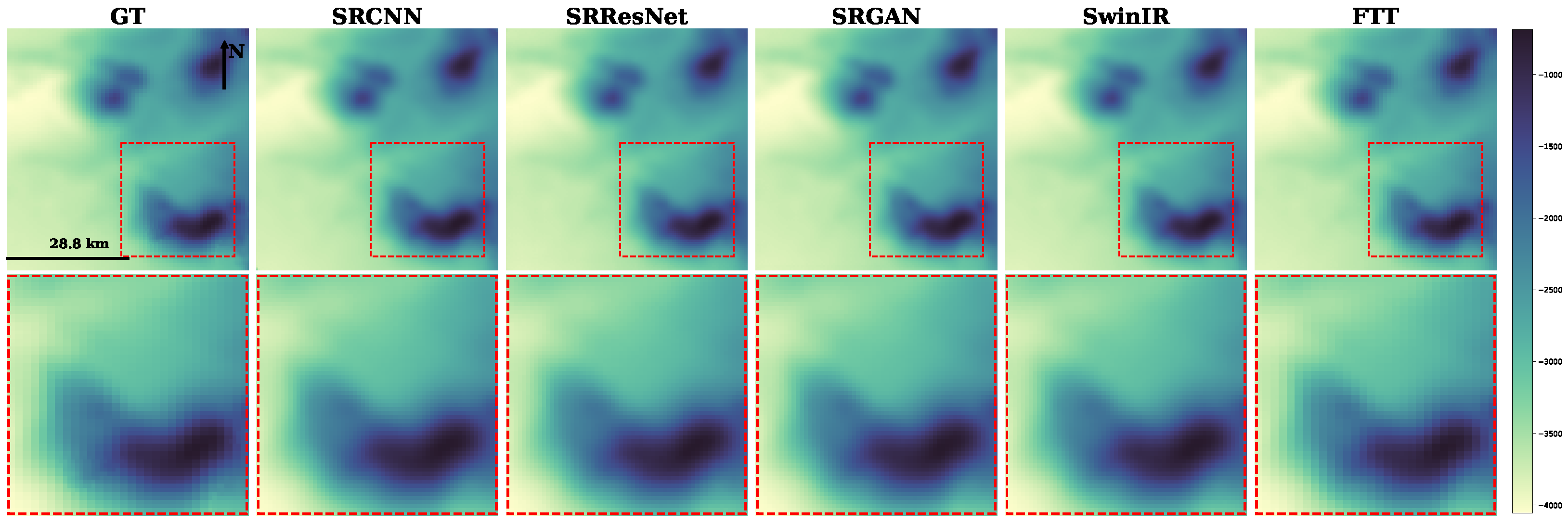
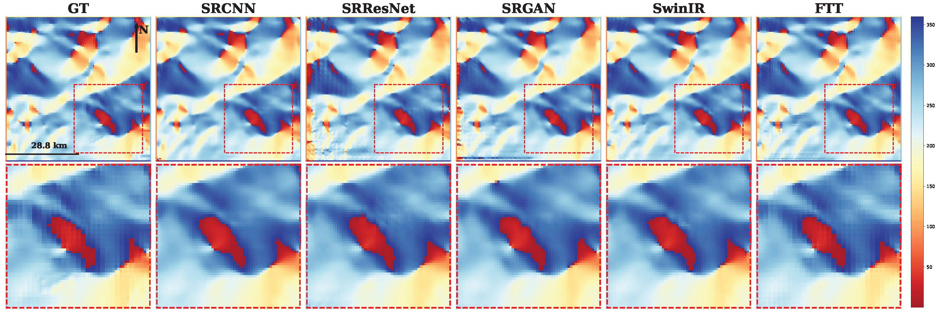
The results of different SR methods on the test set are shown in Table 2. To more intuitively show the performance of different models, we randomly selected a patch from the test set to show the reconstruction effect of elevation (Figure 5), slope (Figure 6), and aspect (Figure 7).
As shown in Table 2, FTT demonstrates the best performance across all four evaluation metrics, highlighting its effectiveness at enhancing the precision of generated HR DBM. Among the three methods using CNN, SRCNN performs relatively poorly in elevation RMSE due to the limitation of fewer convolutional layers, but its slope RMSE and aspect RMSE slightly exceed those of SRResNet and SRGAN, possibly because SRCNN takes a bicubic interpolated value as input. SRGAN outperforms SRResNet, suggesting that perceptual loss functions can improve reconstruction accuracy to some extent, but the SSIM metrics are not improved compared to the other two methods. SwinIR outperforms the methods using CNN, which demonstrates the superiority of transformers over CNNs, and shows the advantage of a larger receptive field in extracting terrain features.

4. Discussion

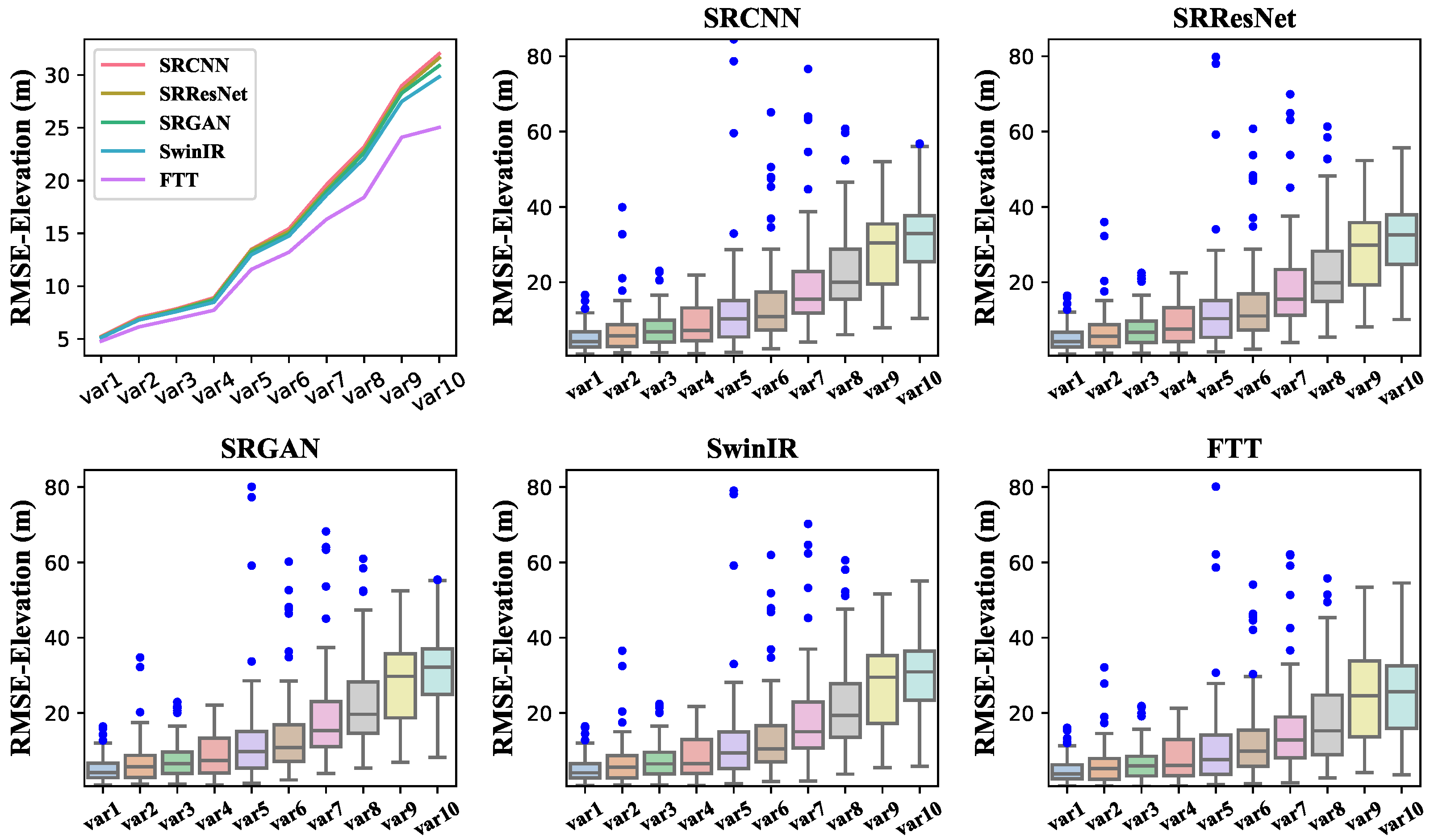
To facilitate a clear comparison of the performance across different models, we utilize boxplots to illustrate the distribution of errors on the test dataset. Specifically, to further exhibit the performance of the various methods under different topographic conditions, we divided the test set into 10 categories based on increasing elevation variance. Variance reflects the degree of terrain undulation. DBM with larger variance represents steeper and more rugged terrains, which typically pose greater challenges for DBM SR. The SR performance of different methods is displayed through box plots (see Figure 8). For ease of comparison, we present an RMSE line chart in the first subplot at the top-left corner of Figure 8. It is evident that all SR methods demonstrate optimal performance on flat terrain and significant limitations on steep terrain, which illustrates that steep and complex terrain presents a significant challenge. The proposed model exhibits superior performance across all terrain types, with a notable reduction in RMSE of 4.89 m compared to SwinIR in the most challenging terrain, indicating that FTT has stronger reconstruction capability and robustness on steep terrains.
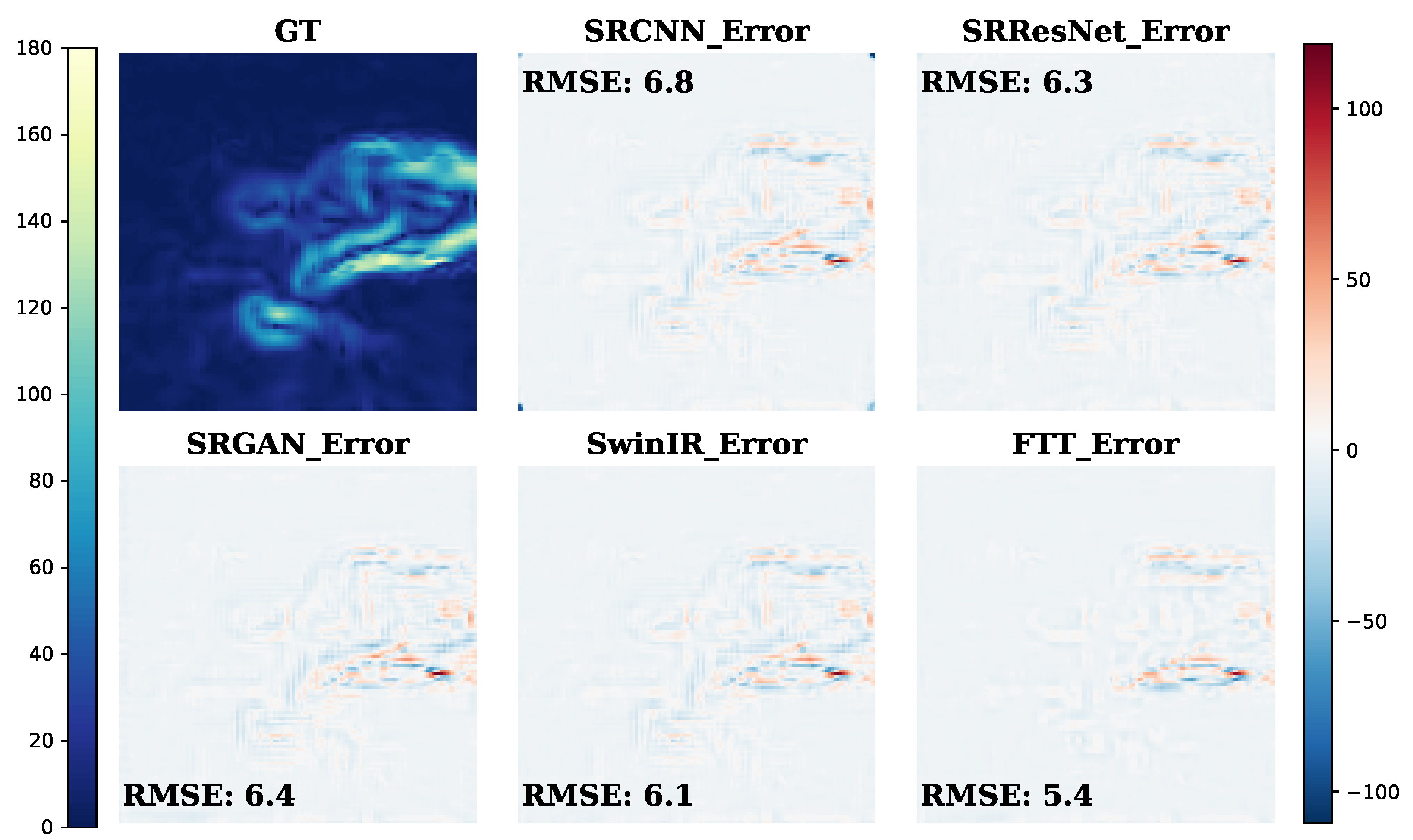
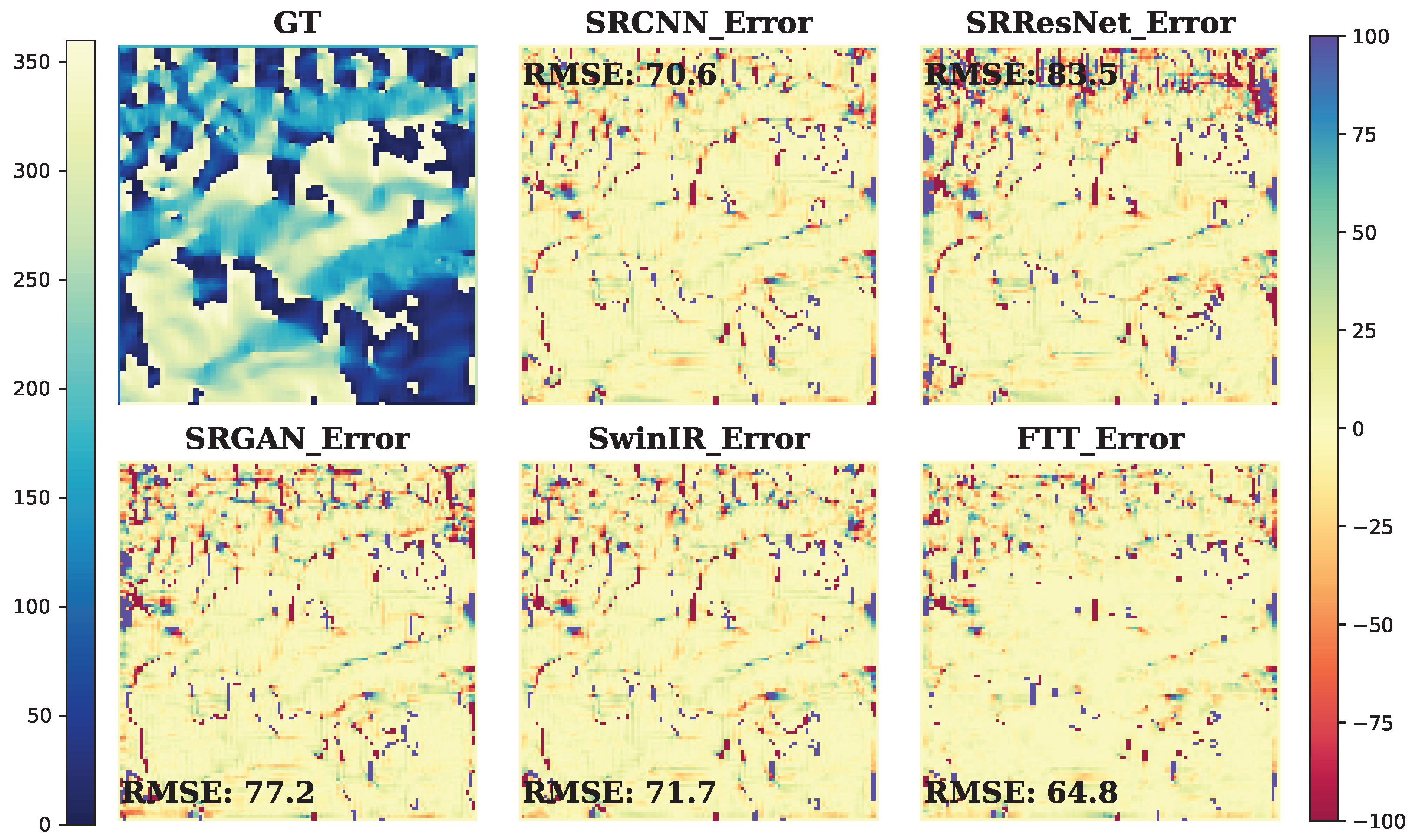
To analyze the spatial distribution characteristics of errors in detail, we randomly selected a sample from the test data, and display its elevation error (Figure 9), slope error (Figure 10), and aspect error (Figure 11). By analyzing the correspondence between errors and actual values in spatial distribution, we conclude that areas with significant terrain undulations often exhibit larger errors and underestimate the true values. This reveals the limitations of CNNs and attention mechanisms regarding such terrains. In contrast, FTT demonstrates a clear advantage in SR reconstruction of steep terrains.

Ablation Experiments

From the above analysis, the proposed FTT method clearly exhibits significant performance advantages in DBM SR reconstruction tasks. To gain a deeper understanding of the specific impact of each key component of the FTT method on overall model performance, and to further validate the rationality of our proposed problem settings, we conducted a series of ablation experiments. We sequentially removed each key component from the FTT to observe the specific impact of these changes on the model’s performance. To ensure fairness and comparability across experiments, we employ identical hyperparameters during training.
Table 3 shows that when only TMB is applied, its SSIM value exceeds that of CA alone. This indicates that TMB effectively enhances image fidelity by utilizing the positional offset generated in shallow features. The inclusion of HFFE results in substantial improvements across all four evaluation metrics, underscoring its effectiveness in extracting high-frequency prior information for DBM SR. The incorporation of CA enhances the model’s ability to perceive two-dimensional spatial features, further optimizing its performance. Collectively, each component functions as intended, contributing to the overall enhancement of performance.

5. Conclusions

Limitations in bathymetry equipment have prompted researchers to use SR technology to generate HR DBMs, but the significant differences between DBMs and natural images are often overlooked, which leads to serious distortions and inaccuracies. We have presented a novel SR method, FTT, to overcome these challenges. We conducted a detailed analysis of the disparities between natural images and terrain, identifying three primary issues prevalent in current SR methods. Subsequently, we proposed the FTT, which includes GTFE, HFFE, and TMB to address these issues. GTFE can aggregate global features and establish long-range dependencies. HFFE enhances the model’s ability to extract high-frequency information. TMB solves the problems of texture distortion and positional offset during upsampling and feature extraction. Experiments demonstrated that the proposed FTT shows significant improvement in elevation, slope, and aspect accuracy compared to commonly used SR models, and exhibits excellent performance, especially in steep terrain. Ablation experiments further validated the effectiveness of each component within FTT. FTT represents a substantial advancement in SR techniques tailored for DBM, offering robust solutions to improve the accuracy and fidelity of HR terrain data generation.
Notably, the error distribution on the test set reveals significant performance differences of all SR methods across various terrains, primarily due to terrain heterogeneity. We acknowledge this phenomenon, but have not extensively explored it, underscoring it as a pivotal area for future investigation. In the future, we intend to comprehensively address terrain differences, and to conduct more nuanced studies aimed at producing highly accurate global HR DBM products.

Author Contributions

Methodology, P.X.; Validation, J.W.; Investigation, Y.W.; Writing—original draft, P.X.; Funding acquisition, J.W. All authors have read and agreed to the published version of the manuscript.

Funding

This research was funded by the National Natural Science Foundation of China, grant number 42375158.

Data Availability Statement

The DBM data used in our paper can be downloaded at: https://www.gebco.net/.

Conflicts of Interest

The authors declare that they have no known competing financial interest or personal relationships that could have appeared to influence the work reported in this paper.

Abbreviations

The following abbreviations are used in this manuscript:
SBESSingle-beam Echo Sounder
MBESMulti-beam Echo Sounder
ALBAirborne LiDAR Bathymetry
SARSynthetic Aperture Radar
SASatellite Altimeter
SDBSatellite-Driven Bathymetry

References

  1. Wölfl, A.C.; Snaith, H.; Amirebrahimi, S.; Devey, C.W.; Dorschel, B.; Ferrini, V.; Huvenne, V.A.I.; Jakobsson, M.; Jencks, J.; Johnston, G.; et al. Seafloor Mapping—The Challenge of a Truly Global Ocean Bathymetry. Front. Mar. Sci. 2019, 6, 283. [Google Scholar] [CrossRef]
  2. Lecours, V.; Dolan, M.F.J.; Micallef, A.; Lucieer, V.L. A review of marine geomorphometry, the quantitative study of the seafloor. Hydrol. Earth Syst. Sci. 2016, 20, 3207–3244. [Google Scholar] [CrossRef]
  3. Chen, H.; Cheng, J.; Ruan, X.; Li, J.; Ye, L.; Chu, S.; Cheng, L.; Zhang, K. Satellite remote sensing and bathymetry co-driven deep neural network for coral reef shallow water benthic habitat classification. Int. J. Appl. Earth Obs. Geoinf. 2024, 132, 104054. [Google Scholar] [CrossRef]
  4. Thompson, A.F.; Sallée, J.B. Jets and Topography: Jet Transitions and the Impact on Transport in the Antarctic Circumpolar Current. J. Phys. Oceanogr. 2012, 42, 956–972. [Google Scholar] [CrossRef]
  5. Ellis, J.; Clark, M.; Rouse, H.; Lamarche, G. Environmental management frameworks for offshore mining: The New Zealand approach. Mar. Policy 2017, 84, 178–192. [Google Scholar] [CrossRef]
  6. He, J.; Zhang, S.; Feng, W.; Lin, J. Quantifying earthquake-induced bathymetric changes in a tufa lake using high-resolution remote sensing data. Int. J. Appl. Earth Obs. Geoinf. 2024, 127, 103680. [Google Scholar] [CrossRef]
  7. Bandini, F.; Olesen, D.; Jakobsen, J.; Kittel, C.M.M.; Wang, S.; Garcia, M.; Bauer-Gottwein, P. Technical note: Bathymetry observations of inland water bodies using a tethered single-beam sonar controlled by an unmanned aerial vehicle. Hydrol. Earth Syst. Sci. 2018, 22, 4165–4181. [Google Scholar] [CrossRef]
  8. Wu, L.; Chen, Y.; Le, Y.; Qian, Y.; Zhang, D.; Wang, L. A high-precision fusion bathymetry of multi-channel waveform curvature for bathymetric LiDAR systems. Int. J. Appl. Earth Obs. Geoinf. 2024, 128, 103770. [Google Scholar] [CrossRef]
  9. Viaña-Borja, S.P.; Fernández-Mora, A.; Stumpf, R.P.; Navarro, G.; Caballero, I. Semi-automated bathymetry using Sentinel-2 for coastal monitoring in the Western Mediterranean. Int. J. Appl. Earth Obs. Geoinf. 2023, 120, 103328. [Google Scholar] [CrossRef]
  10. Sharr, M.B.; Parrish, C.E.; Jung, J. Automated classification of valid and invalid satellite derived bathymetry with random forest. Int. J. Appl. Earth Obs. Geoinf. 2024, 129, 103796. [Google Scholar] [CrossRef]
  11. Li, Z.; Peng, Z.; Zhang, Z.; Chu, Y.; Xu, C.; Yao, S.; Zhu, X.; Yue, Y.; Levers, A.; Zhang, J.; et al. Exploring modern bathymetry: A comprehensive review of data acquisition devices, model accuracy, and interpolation techniques for enhanced underwater mapping. Front. Mar. Sci. 2023, 10, 1178845. [Google Scholar] [CrossRef]
  12. Mayer, L.; Jakobsson, M.; Allen, G.; Dorschel, B.; Falconer, R.; Ferrini, V.; Lamarche, G.; Snaith, H.; Weatherall, P. The Nippon Foundation—GEBCO Seabed 2030 Project: The Quest to See the World’s Oceans Completely Mapped by 2030. Geosciences 2018, 8, 63. [Google Scholar] [CrossRef]
  13. Farsiu, S.; Robinson, D.; Elad, M.; Milanfar, P. Advances and challenges in super-resolution. Int. J. Imaging Syst. Technol. 2004, 14, 47–57. [Google Scholar] [CrossRef]
  14. Zhang, X.; Zhang, W.; Guo, S.; Zhang, P.; Fang, H.; Mu, H.; Du, P. UnTDIP: Unsupervised neural network for DEM super-resolution integrating terrain knowledge and deep prior. Int. J. Appl. Earth Obs. Geoinf. 2023, 122, 103430. [Google Scholar] [CrossRef]
  15. Zhou, A.; Chen, Y.; Wilson, J.P.; Chen, G.; Min, W.; Xu, R. A multi-terrain feature-based deep convolutional neural network for constructing super-resolution DEMs. Int. J. Appl. Earth Obs. Geoinf. 2023, 120, 103338. [Google Scholar] [CrossRef]
  16. Wang, Y.; Jin, S.; Yang, Z.; Guan, H.; Ren, Y.; Cheng, K.; Zhao, X.; Liu, X.; Chen, M.; Liu, Y.; et al. TTSR: A transformer-based topography neural network for digital elevation model super-resolution. IEEE Trans. Geosci. Remote Sens. 2024, 62, 4403719. [Google Scholar] [CrossRef]
  17. Dong, C.; Loy, C.C.; He, K.; Tang, X. Image Super-Resolution Using Deep Convolutional Networks. arXiv 2015, arXiv:1501.00092. [Google Scholar] [CrossRef]
  18. Jiao, J.; Tu, W.C.; He, S.; Lau, R.W.H. FormResNet: Formatted Residual Learning for Image Restoration. In Proceedings of the 2017 IEEE Conference on Computer Vision and Pattern Recognition Workshops (CVPRW), Honolulu, HI, USA, 21–26 July 2017; pp. 1034–1042. [Google Scholar] [CrossRef]
  19. Fan, Y.; Shi, H.; Yu, J.; Liu, D.; Han, W.; Yu, H.; Wang, Z.; Wang, X.; Huang, T. Balanced Two-Stage Residual Networks for Image Super-Resolution. In Proceedings of the 30th IEEE Conference on Computer Vision and Pattern Recognition Workshops, CVPRW 2017, Honolulu, HI, USA, 21–26 July 2017; pp. 1157–1164. [Google Scholar] [CrossRef]
  20. Tai, Y.; Yang, J.; Liu, X.; Xu, C. MemNet: A Persistent Memory Network for Image Restoration. arXiv 2017, arXiv:1708.02209. [Google Scholar] [CrossRef]
  21. Ren, H.; El-Khamy, M.; Lee, J. Image Super Resolution Based on Fusing Multiple Convolution Neural Networks. In Proceedings of the 2017 IEEE Conference on Computer Vision and Pattern Recognition Workshops (CVPRW), Honolulu, HI, USA, 21–26 July 2017; pp. 1050–1057. [Google Scholar] [CrossRef]
  22. Li, W.; Tao, X.; Guo, T.; Qi, L.; Lu, J.; Jia, J. MuCAN: Multi-Correspondence Aggregation Network for Video Super-Resolution. arXiv 2020, arXiv:2007.11803. [Google Scholar]
  23. Tong, T.; Li, G.; Liu, X.; Gao, Q. Image Super-Resolution Using Dense Skip Connections. In Proceedings of the 2017 IEEE International Conference on Computer Vision (ICCV), Venice, Italy, 22–29 October 2017; pp. 4809–4817. [Google Scholar] [CrossRef]
  24. Guo, Y.; Chen, J.; Wang, J.; Chen, Q.; Cao, J.; Deng, Z.; Xu, Y.; Tan, M. Closed-Loop Matters: Dual Regression Networks for Single Image Super-Resolution. In Proceedings of the 2020 IEEE/CVF Conference on Computer Vision and Pattern Recognition (CVPR), Seattle, WA, USA, 13–19 June 2020; pp. 5406–5415. [Google Scholar] [CrossRef]
  25. Shocher, A.; Cohen, N.; Irani, M. Zero-Shot Super-Resolution Using Deep Internal Learning. In Proceedings of the 2018 IEEE/CVF Conference on Computer Vision and Pattern Recognition, Salt Lake City, UT, USA, 18–23 June 2018; pp. 3118–3126. [Google Scholar] [CrossRef]
  26. Xu, Y.S.; Tseng, S.Y.R.; Tseng, Y.; Kuo, H.K.; Tsai, Y.M. Unified Dynamic Convolutional Network for Super-Resolution with Variational Degradations. arXiv 2020, arXiv:2004.06965. [Google Scholar] [CrossRef]
  27. Ledig, C.; Theis, L.; Huszar, F.; Caballero, J.; Cunningham, A.; Acosta, A.; Aitken, A.; Tejani, A.; Totz, J.; Wang, Z.; et al. Photo-Realistic Single Image Super-Resolution Using a Generative Adversarial Network. arXiv 2017, arXiv:1609.04802. [Google Scholar]
  28. Wang, X.; Yu, K.; Wu, S.; Gu, J.; Liu, Y.; Dong, C.; Loy, C.C.; Qiao, Y.; Tang, X. ESRGAN: Enhanced Super-Resolution Generative Adversarial Networks. arXiv 2018, arXiv:1809.00219. [Google Scholar] [CrossRef]
  29. Wang, X.; Xie, L.; Dong, C.; Shan, Y. Real-ESRGAN: Training Real-World Blind Super-Resolution with Pure Synthetic Data. arXiv 2021, arXiv:2107.10833. [Google Scholar]
  30. Ma, X.; Li, H.; Chen, Z. Feature-Enhanced Deep Learning Network for Digital Elevation Model Super-Resolution. IEEE J. Sel. Top. Appl. Earth Obs. Remote Sens. 2023, 16, 5670–5685. [Google Scholar] [CrossRef]
  31. Park, N.; Kim, S. How Do Vision Transformers Work? arXiv 2022, arXiv:2202.06709. [Google Scholar] [CrossRef]
  32. Li, A.; Zhang, L.; Liu, Y.; Zhu, C. Feature Modulation Transformer: Cross-Refinement of Global Representation via High-Frequency Prior for Image Super-Resolution. In Proceedings of the 2023 IEEE/CVF International Conference on Computer Vision (ICCV), Paris, France, 1–6 October 2023; pp. 12480–12490. [Google Scholar] [CrossRef]
  33. Zhou, Y.; Li, Z.; Guo, C.L.; Liu, L.; Cheng, M.M.; Hou, Q. SRFormerV2: Taking a Closer Look at Permuted Self-Attention for Image Super-Resolution. arXiv 2024, arXiv:2303.09735. [Google Scholar]
  34. Shi, W.; Caballero, J.; Huszár, F.; Totz, J.; Aitken, A.P.; Bishop, R.; Rueckert, D.; Wang, Z. Real-Time Single Image and Video Super-Resolution Using an Efficient Sub-Pixel Convolutional Neural Network. arXiv 2016, arXiv:1609.05158. [Google Scholar]
  35. Liu, Z.; Lin, Y.; Cao, Y.; Hu, H.; Wei, Y.; Zhang, Z.; Lin, S.; Guo, B. Swin Transformer: Hierarchical Vision Transformer using Shifted Windows. arXiv 2021, arXiv:2103.14030. [Google Scholar] [CrossRef]
  36. Hou, Q.; Zhou, D.; Feng, J. Coordinate Attention for Efficient Mobile Network Design. In Proceedings of the 2021 IEEE/CVF Conference on Computer Vision and Pattern Recognition (CVPR), Nashville, TN, USA, 20–25 June 2021; pp. 13708–13717. [Google Scholar] [CrossRef]
  37. Jiang, Y.; Xiong, L.; Huang, X.; Li, S.; Shen, W. Super-resolution for terrain modeling using deep learning in high mountain Asia. Int. J. Appl. Earth Obs. Geoinf. 2023, 118, 103296. [Google Scholar] [CrossRef]
  38. Cai, W.; Liu, Y.; Chen, Y.; Dong, Z.; Yuan, H.; Li, N. A Seabed Terrain Feature Extraction Transformer for the Super-Resolution of the Digital Bathymetric Model. Remote Sens. 2023, 15, 4906. [Google Scholar] [CrossRef]
  39. Zhang, B.; Xiong, W.; Ma, M.; Wang, M.; Wang, D.; Huang, X.; Yu, L.; Zhang, Q.; Lu, H.; Hong, D.; et al. Super-resolution reconstruction of a 3 arc-second global DEM dataset. Sci. Bull. 2022, 67, 2526–2530. [Google Scholar] [CrossRef]
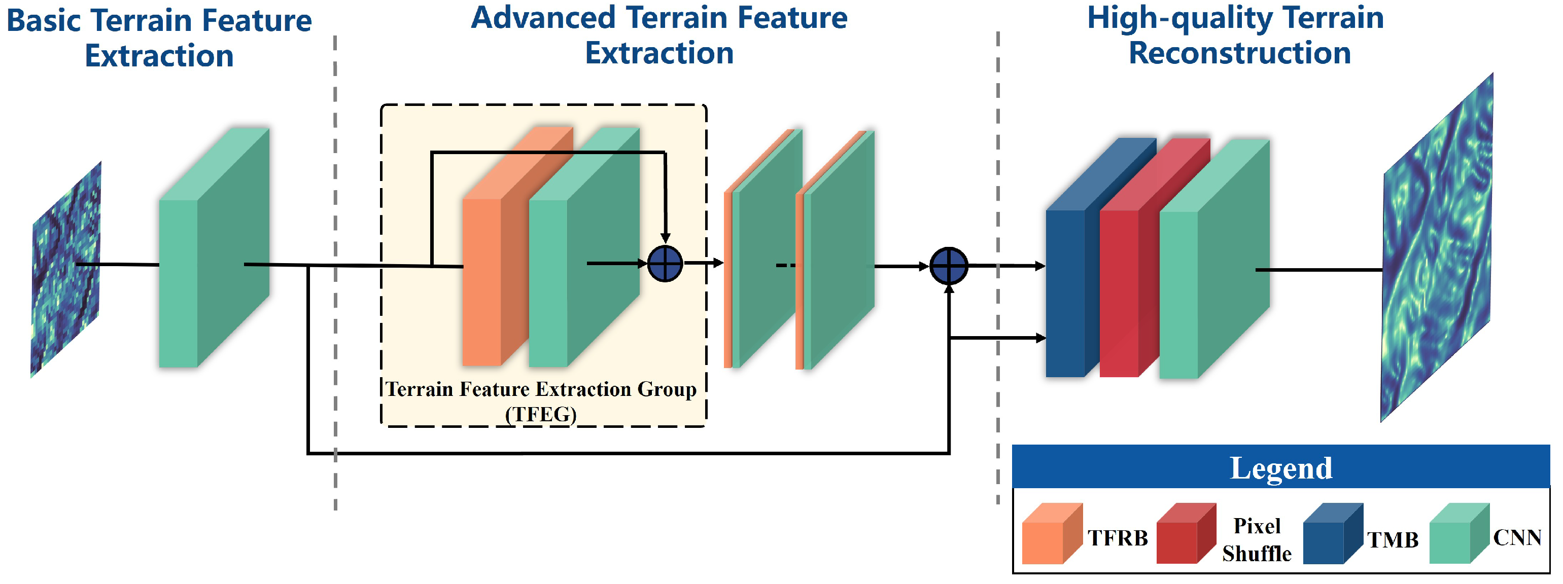
Figure 1. The overall architecture of the proposed FTT.
Jmse 13 01365 g001
Figure 2. Core components of FTT. (a) Terrain Feature Refining Block (TFRB), (b) Global Terrain Feature Extraction (GTFE), (c) High-frequency Feature Extraction (HFFE), (d) Terrain Matching Block (TMB).
Jmse 13 01365 g002
Figure 3. Principle of coordinate attention. r represents the compression ratio of the channel.
Jmse 13 01365 g003
Figure 4. Display of the selected ocean area: (a) filled map of the selected ocean area; (b) elevation frequency of the selected ocean area.
Jmse 13 01365 g004
Figure 5. Comparison of the elevation in HR DBM reconstructed by five different models (red box represents the magnified details).
Jmse 13 01365 g005
Figure 6. Comparison of the slope in HR DBM reconstructed by five different models (red box represents the magnified details).
Jmse 13 01365 g006
Figure 7. Comparison of the aspect in HR DBM reconstructed by five different models (red box represents the magnified details).
Jmse 13 01365 g007
Figure 8. Error distribution of various models across different levels of variance.
Jmse 13 01365 g008
Figure 9. Elevation error spatial distribution of different models.
Jmse 13 01365 g009
Figure 10. Slope error spatial distribution of different models.
Jmse 13 01365 g010
Figure 11. Aspect error spatial distribution of different models.
Jmse 13 01365 g011
Table 1. Comparison of three prevailing bathymetry methods.
MethodsSensorsStrengthLimitations
ShipborneSBESHighly reliableLimited range
MBESHigh resolutionHigh operating costs
AirborneALBHigh accuracyLimited water depth
SARIgnore clouds and fogHigh uncertainty
SpaceborneSAWide rangeLow accuracy
SDBWide rangeLimited water depth
Table 2. Performance comparison results of DBM SR.
ModelRMSE of
Elevation (m) ↓
RMSE of
Slope (°) ↓
RMSE of
Aspect (°) ↓
SSIM ↑
SRCNN16.305.2968.290.968
SRResNet16.075.3971.060.968
SRGAN16.235.1968.100.968
SwinIR15.435.1267.430.969
FTT (ours)13.484.8165.250.973
↓ indicates that a lower value of the indicator is better; ↑ indicates that a higher value of the indicator is better.
Table 3. Result of the ablation experiment.
CAHFFETMBRMSE of Elevation (m) ↓RMSE of Slope (°) ↓RMSE of Aspect (°) ↓SSIM ↑
I 13.904.9165.740.972
II 13.794.8865.530.973
III 13.934.9266.110.973
IV 13.764.8765.650.973
V 13.844.9065.550.973
VI 13.764.8765.510.973
VII13.484.8164.970.973
↓ indicates that a lower value of the indicator is better; ↑ indicates that a higher value of the indicator is better; ✓ denotes that the component is in use.
Disclaimer/Publisher’s Note: The statements, opinions and data contained in all publications are solely those of the individual author(s) and contributor(s) and not of MDPI and/or the editor(s). MDPI and/or the editor(s) disclaim responsibility for any injury to people or property resulting from any ideas, methods, instructions or products referred to in the content.