A Crossover Adjustment Method Considering the Beam Incident Angle for a Multibeam Bathymetric Survey Based on USV Swarms

Abstract

Multibeam echosounder systems (MBESs) are widely used in unmanned surface vehicle swarms (USVs) to perform various marine bathymetry surveys because of their excellent performance. To address the challenges of systematic error superposition and edge beam error propagation in multibeam bathymetry surveying, this study proposes a novel error adjustment method integrating crossover error density clustering and beam incident angle (BIA) compensation. Firstly, a bathymetry error detection model was developed based on adaptive Density-Based Spatial Clustering of Applications with Noise (DBSCAN). By optimizing the neighborhood radius and minimum sample threshold through analyzing sliding-window curvature, the method achieved the automatic identification of outliers, reducing crossover discrepancies from ±150 m to ±50 m in the deep sea at a depth of approximately 5000 m. Secondly, an asymmetric quadratic surface correction model was established by incorporating the BIA as a key parameter. A dynamic weight matrix ω = 1/(1 + 0.5θ²) was introduced to suppress edge beam errors, combined with Tikhonov regularization to resolve ill-posed matrix issues. Experimental validation in the Western Pacific demonstrated that the RMSE of crossover points decreased by about 30.4% and the MAE was reduced by 57.3%. The proposed method effectively corrects residual systematic errors while maintaining topographic authenticity, providing a reference for improving the quality of multibeam bathymetric data obtained via USVs and enhancing measurement efficiency.

1. Introduction

Seabed topography data represent fundamental information guiding the utilization of marine environmental resources and the environmental upkeep of naval battlefields [1,2,3,4]. Shipborne multibeam bathymetry technology is currently one of the important means of assessing seabed topography and geomorphology [5,6]. Multibeam echosounder systems (MBESs) can obtain high-precision and high-resolution underwater topography information [7,8,9], which plays an important role in ensuring the navigation safety of marine surface and underwater vessels. With the development of unmanned ships and swarm control technologies, unmanned surface vehicle swarms (USVs) equipped with an MBES have been widely applied to perform various marine bathymetry surveying tasks due to their excellent performance [10,11,12,13,14].

However, while the accompanying multibeam bathymetric survey technology improves the efficiency of the MBES, it also introduces the problem of multi-source heterogeneous data fusion, as follows:

(1)

The coordination of USVs leads to the superposition of systematic errors.

(2)

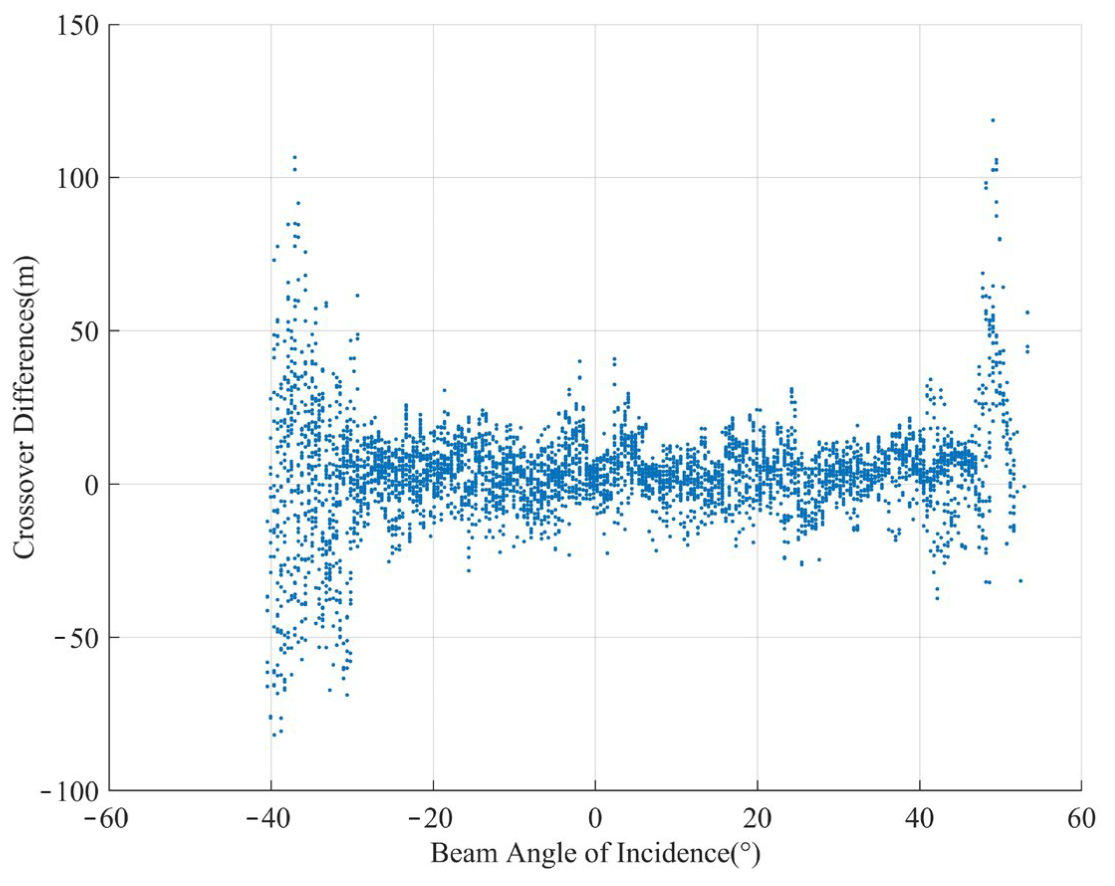
The error propagation of the incident angle of the edge beam intensifies in the MBES.

The bathymetric data errors caused by the above-mentioned problems are mainly reflected in the discrepancies at the crossover points of the measurement lines in the data post-processing stage. In order to effectively reduce the measurement errors in bathymetric data, the outliers among them should be eliminated first. Outliers in depth sounding can significantly affect the effect of model correction. Yang et al. [15] removed depth outliers using depth-gradient thresholding. Rezvani et al. [16] processed multibeam bathymetric data based on M-estimators. Weighting the data around the water depth points effectively weakens the adverse effects of peripheral observations and improves the robustness of the data. Ferreira et al. [17] used the Spatial Outliers Detection Algorithm (SODA) to process multibeam bathymetric data, considering the autocorrelation and non-normality of the data, and effectively improved the speed of data processing. Density-Based Spatial Clustering of Applications with Noise (DBSCAN) is a good method and can effectively detect outliers in the data. DBSCAN was selected over alternative clustering methods (e.g., OPTICS, HDBSCAN, and model-based approaches) due to its dual advantages of handling spatially irregular point densities and inherent robustness to noise [18,19]. Given the high noise-to-signal ratio in our dataset and the non-uniform distribution of sampling points, DBSCAN’s density-based paradigm provides superior resilience against outlier contamination while requiring no a priori assumptions about cluster geometry. Therefore, in this study, DBSCAN is utilized to handle outliers in the crossover point data, further enhancing the data robustness.

After eliminating the outlier data in the depth, a depth correction model is established for data correction. Li et al. [20] proposed a marine sounding network adjustment method for marine measurement data based on the traditional method of geodetic network adjustment, which improved the discrepancies in the crossover point difference values in the single-ship measurement mode. An assumption of equally weighted least squares was adopted; this does not conform to the error distribution characteristics of the edge beam. Considering the multi-source, heterogeneous, and massive characteristics of multibeam seabed topographic survey results, Huang et al. [21] presented a method of constructing seabed topographic surfaces based on triangulation networks and calculated the crossover point differences at all depths, which improved efficiency when processing massive amounts of data. Xu et al. [22] proposed a position-dependent quadratic surface model to correct the depth error. However, the traditional error correction model of multibeam bathymetric data only considers the relationship between the depth difference value and the geographical coordinates, and does not consider the influence of different beam incident angles (BIAs) on the depth value.

Therefore, this study proposes a crossover adjustment method that integrates clustering of the error density of sounding points and BIA compensation. The main procedures and characteristics are as follows:

(1)

A gross error detection model is constructed based on machine learning. The adaptive Density-Based Spatial Clustering of Applications with Noise (DBSCAN) algorithm is proposed. Dynamically optimizing the neighborhood radius Eps and the minimum sample number of parameters MinPts enables the intelligent recognition of gross errors in crossover point differences.

(2)

An incident angle-weighted error compensation model is established. Taking the incident angle function as the weight, an improved depth crossover difference quadratic surface model is constructed to suppress the edge error effect of multiple beams.

(3)

A regularized weighted least-squares framework is designed. The Tikhonov regularization matrix is introduced to effectively solve the pathological problem of the normal equation and ensure the stability of the solution after calculations with large volumes of data.

The method proposed in this paper can effectively improve the quality of measurement data, further enhance the efficiency of data transformation, and provide a feasible reference for handling bathymetric data.

This article is structured as follows: In Section 2, we propose a new crossover adjustment method. Through an adaptive DBSCAN algorithm and incident angle-weighted error compensation model, the residual systematic errors in the bathymetric data are further eliminated. Section 3 introduces the experimental procedures, experimental data, and experimental areas in detail and presents the quality assessment indicators. In Section 4, the reliability of the proposed method is demonstrated by comparing the results for the correction of multibeam bathymetric data obtained using different methods and their influences on seabed topography. Finally, Section 5 presents our conclusions.

2. Methods

This section presents the methodological framework for crossover error adjustment in multibeam bathymetry. The primary objectives are (1) to develop an adaptive DBSCAN algorithm for automatic outlier detection, (2) to establish a beam incident angle-weighted correction model addressing edge beam errors, and (3) to design a regularized weighted least-squares solver ensuring stability when processing large volumes of data.

2.1. Error Elimination Method for Multibeam Bathymetry Data Based on Adaptive DBSCAN

Errors that occur in the process of collecting bathymetric data using multibeam echosounder systems are classified as systematic errors, random errors, or gross errors [23,24,25]. Systematic errors mainly comprise the overall deviations in measurement data caused by instrument installation deviations, sound speed profile errors, attitude errors, etc. These errors can be effectively weakened or eliminated through corresponding corrections during the processing of measurement data. Random errors are caused by factors such as the accuracy of the measuring instrument and environmental dynamics. Their value is generally low, and the error within the range specified by the measurement specification can be retained without affecting the final measurement result. Gross errors often take the form of deviations from the main bathymetric depth clusters during data processing and can usually be precisely identified and proposed through manual processing or automatic cleaning algorithms. In order to reduce the interference from various errors on the test results, the data used in this paper have undergone all corrections and errors have been basically eliminated from the USV measurement through manual discrimination.

The comparison of the crossover points of the main measurement lines represents one of the key methods for verifying the quality of MBES data [26]. This method determines whether the measurement data meet the measurement requirements by using two mutually perpendicular measurement lines, comparing the depth values at the same position, and calculating the proportion of the total number of depths whose crossover point difference exceeds the limit for difference requirements stipulated in the specification for the total number of depths.

However, during the comparison process for the crossover points of the main USV multibeam measurement lines, although the measurement data for the main measurement lines involved in the comparison had all undergone fine data processing, we found that there were always large residual errors in the crossover point differences. These gross errors were mainly caused by residual depth errors, due to, for example, positioning accuracy errors, sound velocity correction errors, and attitude correction errors. This ultimately affected the quality of the overall data, as shown in Figure 1.

It can be seen from Figure 1 that the discrepancies at the crossover points are generally distributed in a band-like pattern, mainly concentrated in the middle area. Most are randomly distributed around 0, with differences within a 50 m range. Some larger differences are distributed at the periphery of the data. The maximum absolute value of the differences exceeds 100 m, which greatly affects the quality of the data. In order to further eliminate gross errors, based on the data distribution in Figure 1, the greater the distance between the crossover points, the more the density of the bathymetric data rises. The range of discrepancies in the crossover points continues expanding, and certain category characteristics can be observed. The cluster analysis method can quickly identify noise, eliminate erroneous data showing a low correlation with the majority of the central data, and improve the quality of the data. Unlike partitional (e.g., k-means) or hierarchical methods, DBSCAN eliminates the need to predefine cluster counts, which is impractical for our exploratory analysis. Although HDBSCAN is capable of managing variable densities, it introduces unnecessary complexity for our distinct noise-separation objective. Model-based clustering was deemed inappropriate due to its parametric distribution assumptions, which contradict our dataset’s heterogeneity. Therefore, this paper proposes a gross error elimination method for multibeam data based on DBSCAN to eliminate the influence of residuals in crossover point data on multibeam data.

DBSCAN is a density-based spatial clustering algorithm through which clusters of any shape and size can be discovered in a database containing uniform noise and outliers [27,28,29]. For each object in a certain cluster, the number of data objects within the neighborhood of a given radius, defined by Eps, must be greater than a given value. Namely, the neighborhood density must exceed a certain threshold, denoted as MinPts. The points within the neighborhood of the core point form clusters with an achievable density. The boundary points are located at the edge of the clusters but do not meet the core conditions, and the remaining points are regarded as noise. This algorithm does not require a preset number of clusters and can discover clusters of any shape, such as non-spherical structures, but is sensitive to the parameters Eps and MinPts. Its effect is limited when high-dimensional data or densities change sharply. Its advantages lie in its strong anti-noise ability and in not requiring prior assumptions, and it is suitable for scenarios such as geographic information analysis and anomaly detection [30]. In order to effectively identify gross errors, two parameters, Eps and MinPts, need to be manually selected before clustering. Therefore, this paper proposes an adaptive parameter determination method based on the sliding-window average curvature method for setting appropriate parameters. A larger MinPts value can enhance the representativeness of the data. In this paper, 2–5% of the total data size is selected as the value of MinPts. After determining the value of the parameter MinPts, the value of the other parameter Eps is determined based on the value at the inflection point of the k-distance curve. The k-distance [31,32] curve refers to the following process: in a given dataset $D$, for any $D(i)$, the distance is calculated between $D(i)$ and all points in a subset P of the set $D$, and the distances are arranged in ascending order. If the sorted set of distances is denoted as $L$, then $L(k)$ is called the k-distance; that is to say, the KTH closest distance between point $D(i)$ at time $L(k)$ and all points (excluding itself). By calculating the k-distance for all points in the dataset $D$, it is finally possible to obtain the set $E$ of the k-distance for all points. Afterward, based on the k-distance set $E$ of all the obtained points, all the data in the set $D$ are sorted in ascending order to obtain $E^{*}$. The sorted distance set is fitted into a variation curve graph of k-distance, and it is possible to determine the value of k-distance corresponding to the position that changes sharply, that is, the inflection point value, as the value of the radius parameter Eps.

There are three main methods of obtaining the inflection point of the k-distance curve. In the process of obtaining the Eps value using the k-distance curve, it is necessary to determine the value at the inflection point of the curve. These methods are the gradient method [33], the second-order differential method [34], and the sliding-window mean curvature method [35]. The gradient method refers to finding the first-order difference of the smoothed data to locate the parameter value corresponding to the maximum gradient point. The second-order differential method refers to the new sequence obtained by performing two difference operations on a sequence, that is, to determine the rate of change of the difference between two adjacent points and identify the position with the greatest change, which is the inflection point. The sliding-window averaging method sets the width of the sliding window, uses quadratic polynomials to fit the data within the window, and then calculates the quadratic derivative of the data within the window. Compared with the gradient method, it can better capture the characteristics of inflection points and improve the accuracy of detection. Therefore, this paper proposes a method for determining the Eps value based on the moving-window average to improve the stability and efficiency of the proposed adaptive DBSCAN algorithm. We let the k-distance curve be a discrete sequence and $D$ be

$$D={\left\{d_i\right\}}_{i=1}^N$$

(1)

where $d_i$ represents the distance from the i-th sample point to its k-nearest neighbor.

The inflection point of the k-distance curve is obtained using the sliding-window averaging method.

Firstly, the sliding-window operator is set. For a given window width w, the sliding average sequence $\left\{{\overline{d}}_i\right\}$ satisfies

$${\overline{d}}_i={\displaystyle \frac{1}{w}}{\displaystyle \sum _{j=1-w/2}^{i+w/2}{d}_j}$$

(2)

In order to solve the problems of unstable fitting and low computational efficiency caused by setting a fixed size for window size, this paper proposes the principle of optimal window selection, as shown in Equation (3). By minimizing the variance of the curvature sequence, the optimal window value $w_{opt}$ is obtained to improve the accuracy and efficiency of the calculation.

$$w_{opt}=\underset{w}{\min }\left[\mathrm{MSE}(w)+\gamma \cdot \mathrm{Variation}(w)\right]$$

(3)

where $\mathrm{MSE}(w)={\displaystyle \frac{1}{N}}{{\displaystyle {\sum }_{i=1}^N\left(d_i-{\overline{d}}_i\right)}}^2$ is the mean square deviation, $\gamma =0.5$ is the empirical coefficient, and $\mathrm{Variation}(w)={\displaystyle {\sum }_{i=2}^N\left|{\overline{d}}_i-{\overline{d}}_{i-1}\right|}$ measures the volatility of the curve.

The sliding-window sequence is obtained based on the determined window size, and the first-order difference sequence $\left\{{\epsilon }_i\right\}$ is calculated as

$${\epsilon }_i={\overline{d}}_{i+1}-{\overline{d}}_i$$

(4)

We then search the point of maximum gradient change $i_{\max }$ according to

$$i_{\max }=\underset{1\le i\le (N-1)}{\max }\left|{\epsilon }_{i+1}-{\epsilon }_i\right|$$

(5)

Finally, the distance value in the moving average sequence is obtained based on the sequence number $i_{\max }$ at the maximum value of the gradient change, which is the value of the parameter Eps, as follows:

$$Eps={\overline{d}}_{i_{\max }}$$

(6)

During cluster analysis, based on the determined parameters Eps and MinPts, noise data are marked as −1 and regarded as invalid data. All the remaining bathymetric data are classified into one category and labeled with the number 1 as valid data. The valid bathymetric data marked as 1 are saved for the calculation of the crossover point difference.

2.2. Error Correction Method for Quadratic Surface Model of Bathymetric Data Based on BIA

2.2.1. The Quadratic Surface Error Correction Model for Bathymetric Data Considering the BIA

For MBES bathymetry data with overlapping areas, due to the influence of various errors, there are always differences in the depth values at the crossover points. In order to improve the accuracy of low-precision data, the overall correction of the data is carried out based on the idea of depth sounding network adjustment through the overlapping area between the data and the high-precision data. In previous studies, the quadratic surface function related to the depth sounding error and position was mainly constructed for the correction of multibeam depth sounding data [36], as shown in Equation (7).

$$\delta =F(x,y)=a_0+a_{1}x+a_{2}y+a_3{x}^2+a_4{y}^2+a_{5}xy$$

(7)

where $\delta =F(x,y)$ is the multibeam sounding error, which is the difference at the crossover points at the same position. x and y are the planar coordinates of the depth measurement points. $a_0~a_5$ is the undetermined parameter of the model.

The traditional MBES error model, as shown in Equation (7), only considers the error component related to the plane position and ignores the influence of the BIA. The incident angle has a significant influence on the multibeam measurement results. The larger the incident angle, the more significant the deviation of the sound wave propagation path from the vertical direction. The depth measurement error caused by the sound velocity error increases exponentially with the increase in the incident angle. By analyzing the distribution relationship between the incident angle of the beam and the difference at the crossover points, the results shown in Figure 2 are obtained.

As can be seen in Figure 2, in terms of the distribution of depth errors, the crossover point difference for the central beam is below 50 m, while the crossover point difference for the edge beam has undergone a significant mutation, with the maximum difference exceeding 100 m, significantly affecting the overall quality of the data. This indicates that there are residual values related to the BIA in the measurement data. Therefore, in this paper, through the addition of the BIA, as an important parameter, to the traditional model, the ability of the model to adapt to complex terrain changes is improved. The depth error correction model based on incident angle compensation is established as

$${\delta }_{new}={\displaystyle \sum _{k=0}^9{a}_k{\varphi }_k(x,y,\theta )}, {\varphi }_k\in \left\{1,x,y,x^2,y^2,xy,\theta ,{\theta }^2,\theta x,\theta y\right\}$$

(8)

where the multibeam sounding error ${\delta }_{new}$ is the difference at the crossover points at the same position, $\theta$ is the BIA of multibeam data, $a_0$ is the reference value for systematic error, $a_1~a_5$ is the component of the planar position-related error, and $a_6~a_9$ is the error component related to the BIA.

It can be deduced from Equation (8) that the mathematical model for multibeam sounding is

$$z=z_0+F(x,y,\theta )+\Delta$$

(9)

If there are N crossover points in the main inspection comparison, the correction number of z is v, and the depth value of the inspection line is $z^j$; then, according to the common points of the inspection line and the main measurement line at the same position, the following error equation can be established:

$$v_i=(z_i-z_i^j)-{\delta }_{new(i)}+\Delta$$

(10)

where i represents the serial number of the common point in the overlapping area of the measurement line and the main measurement line, and $\Delta$ is the random error. Equation (10) can be written in matrix form as

$$V=AX-L$$

(11)

where V is the vector composed of the difference between the depth measurement values for the inspection line at the common point and those of the main survey line, X is the vector of the parameters to be determined in the systematic error model, A is the coefficient matrix, and L is the vector of the difference between the observed values for the inspection line and the main survey line at the common point.

The least-squares adjustment method is widely applied in processing bathymetry data errors [37,38]. The least-squares solution for the model parameters can be expressed as

$$X={(A^{T}PA)}^{-1}{A}^{T}PL$$

(12)

where P represents the weight matrix of the observed values.

In the solution process of the quadratic surface method, it is assumed that the coincident depth measurement points are of equal precision and that the corresponding weight matrix P is the identity matrix. According to the criterion of least squares, the vector solution of the systematic error parameter is obtained using Equation (12). Although this method can reasonably solve the problem of the mismatch of sounding data in the area of overlapping strips, the systematic error function obtained does not take into account data outside the overlapping area and does not consider the fusion processing problem for bathymetric data with different accuracies, which is unreasonable. In order to obtain a more accurate expression of the system error, the BIA of the MBES is used to solve the coincident data. In this paper, the BIA weight factor is introduced into the weight array P. The central beam data in the multibeam bathymetric data have the highest accuracy. With an increase in the BIA, the accuracy of the bathymetric data continuously decreases, and there is an inversely proportional relationship between the two [39]. We redefine the diagonal weight matrix P based on the BIA weight factor, as follows:

$$P=diag({\omega }_1,{\omega }_2,\dots ,{\omega }_n)$$

(13)

Lurton [40] proposed the Taylor approximation of the sonar beam footprint distortion model, and it characterizes the relationship between BIA and acoustic signal coherence degradation:

$$Footprint\propto {\displaystyle \frac{1}{\cos \theta }}\approx 1+{\displaystyle \frac{1}{2}}{\theta }^2+o({\theta }^2)$$

(14)

where $o({\theta }^2)$ represents a higher-order infinitesimal of ${\theta }^2$.

Based on the relationship between the beam incident angle and the multi-beam footprint in Equation (14), we take the reciprocal of the second-order Taylor approximation $(1/(1+0.5{\theta }^2))$ as the basis for the selection of depth value weights at different BIAs. Therefore, we assign weights to each depth value based on the size of the BIA, ensuring that the high-precision water depth value of the central beam has a greater influence than the low-precision depth value of the edge beam. The empowerment is as follows:

$${\omega }_i={\displaystyle \frac{1}{1+0.5{\theta }_i^2}},\hspace{1em}i=1,2,\dots ,n.$$

(15)

where ${\theta }_i$ is the BIA, in radians units, at the i-th observation point of the main survey line.

2.2.2. Regularized Weighted Least-Squares Adjustment Method for Crossover Adjustment of Bathymetric Data

In the correction of the depth error using the quadratic surface model, considering the BIA mentioned in the previous section of this paper, 10 model parameters need to be determined. In the deep-sea area, the distribution of depths is relatively sparse, the bathymetric data are affected by instrument errors and environmental interferences, such as waves and multipath effects, and noise is easily mistaken for real seabed topography. Therefore, during the process of fitting the seabed topography surface, the model is prone to overfitting. Moreover, since repeated observations cannot be conducted during the measurement process and repeated observation data cannot be obtained, the observation equation in Equation (11) is pathological. The eigenvalues of the coefficient matrix $A^{T}PA$ of the normal equation monotonically tend to 0, causing a very small observation error to lead to a large deviation in parameter estimation. Therefore, the least-squares solution cannot obtain satisfactory results. In order to prevent the overfitting of the parameters of the depth crossover point difference model and obtain a stable parametric solution, an appropriate regularization method must be adopted [41]. The Tikhonov regularization method is one of the most commonly used regularization methods [42,43,44,45,46]. Based on the classical least-squares criterion, this method adds the condition of minimizing the norm of the parameter vector and simultaneously introduces the regularization matrix and regularization parameters. For the Gauss–Markov linear model [47], the criteria are as follows:

$${(AX-L)}^{\mathrm{T}}P{(AX-L)}^{\mathrm{T}}+\lambda X^{\mathrm{T}}KX=\min$$

(16)

where $\lambda$ is the Tikhonov regularization parameter. K is the regularization matrix.

If the regularization matrix is the identity matrix, then Tikhonov regularization becomes a biased estimation at this time. Therefore, in the process of error correction for multibeam data, the number of measured bathymetric data is huge and the feature dimension of the matrix is too high. By introducing biased estimation, the situation of data overfitting is alleviated and a small amount of deviation is sacrificed to significantly reduce the variance of the data. When measuring in unfamiliar sea areas, we consider that the accuracy of data measured using the same survey line is the same. Therefore, in this study, we use the unit regularization matrix to establish the model. When the uncertainty of the depth value in the measurement area is known, constructing non-trivial regularization matrices based on the uncertainty of the prior water depth can further improve the modeling ability for the area with known seabed topographic data. According to this criterion, the regularization solution can be obtained as follows:

$$X={(A^{T}PA+\lambda I)}^{-1}{A}^{T}PL$$

(17)

where $I$ is an identity matrix of size.

The Tikhonov regularization parameter λ determines the intensity of regularization, and it directly affects the generalization ability and stability of the model [44]. The most commonly used parameter determination methods include the L-curve method [48], the Generalized Cross Validation (GCV) method [49], and the ridge trace method. Based on the number of crossover points in the survey area, this study verifies the advantages and disadvantages of the above three methods on a dataset with 5000 observed values and 10 parameters.

It can be seen from

Table 1. The calculation results of model parameter X and the running time of the algorithm under different methods.

Method	X0	X1	X2	X3	X4	X5	X6	X7	X8	X9	X10	Time/s
L-curve	0.9940	0.9907	0.9962	1.0065	1.0075	0.9900	0.9971	1.0158	1.0106	0.9832	0.9940	0.22
GCV	0.9903	0.9871	0.9923	1.0029	1.0037	0.9862	0.9935	1.0120	1.0069	0.9794	0.9903	8.03
Ridge trace	0.9940	0.9907	0.9962	1.0065	1.0075	0.9900	0.9971	1.0158	1.0106	0.9832	0.9940	0.26
Ture value	1	1	1	1	1	1	1	1	1	1	1	\

that the parameter estimates obtained using the three methods are not considerably different. Among them, the GCV method requires the longest time, while the time required by the L-curve and ridge trace methods is not much different, which is consistent with the results of Wang et al. [50]. Compared with the ridge trace method, the L-curve method is more rigorous in theory and has higher accuracy and better adaptability. Therefore, in this study, the L-curve method is used to determine the regularization parameters. The principle behind the determination of the parameter λ in ill-weighted least-squares adjustment using the L-curve method is that in Equation (17), where both $‖A{X}_{\lambda }-L‖$ and $‖X_{\lambda }‖$ are functions of the regularization parameters $\lambda$. By choosing different $\lambda$ values and plotting with $‖A{X}_{\lambda }-L‖$ as the abscissa and $‖X_{\lambda }‖$ as the ordinate, a series of points ($‖A{X}_{\lambda }-L‖$, $‖X_{\lambda }‖$) are obtained. Through curve fitting, a curve, namely, the L-curve, is obtained. Finally, the value corresponding to the point with the largest curvature on the L-curve is selected as the regularization parameter $\lambda$ to be obtained. The construction function is

$$\eta ={‖X_{\lambda }‖}^2,\rho ={‖A{X}_{\lambda }-L‖}^2$$

(18)

where is the sum of the squares of each element, which is then the square root.

Taking the logarithms of both sides of Equation (17), we obtain

$$\lg \eta =2\lg ‖X_{\lambda }‖,\lg \rho =2\lg ‖A{X}_{\lambda }-L‖$$

(19)

Then, the L-curve is obtained via many $(\rho /2,\eta /2)$ fits. The formula for calculating the curvature of a point on the L-curve is

$$\mu =2{\displaystyle \frac{{\rho }^{\prime }{\eta }^{″}-{\rho }^{″}{\eta }^{\prime }}{{\left[{({\rho }^{\prime })}^2+{({\eta }^{\prime })}^2\right]}^{3/2}}}$$

(20)

where ${\rho }^{\prime }$, ${\eta }^{\prime }$, ${\rho }^{″}$, and ${\eta }^{″}$ are, respectively, the first and second derivatives of $\rho$ and $\eta$, and all are functions of the regularization parameter $\lambda$.

By finding the maximum value for Equation (20), the maximum curvature ${\mu }_{\max }$ of the L-curve can be obtained, and the corresponding value ${\mu }_{\max }$ is the regularization parameter $\lambda$ to be sought. Then, by substituting it into Equation (17), the solution of the equation can be obtained. After determining the value of the Tikhonov regularization parameter $\lambda$, the iterative solution procedures to find the parameter X are as follows:

(1)

Initializing: Taking the ordinary weighted least squares (WLS) solution as the iteration starting point to avoid the convergence instability caused by random initialization, we get

$$X^{(0)}={(A^{T}PA)}^{-1}{A}^{T}PL$$

(21)

(2)

Calculating the residual: We calculate the deviation between the predicted value of the current iterative solution $A{X}^{(k)}$ and the actual observed value L. The absolute value of the residuals $\left|r_i^{(k)}\right|$, shown in (22), is used to dynamically adjust the weights; outliers correspond to large residuals, and the weights decrease. The size of the residuals reflects the fit degree of the model to the data points and guides the subsequent weight update.

$$r^{(k)}=L-A{X}^{(k)}$$

(22)

(3)

Updating the weights: Data points with larger residuals (which may be outliers) have lower weights, weakening their influence on the next round of parameter estimation. In this study, the principle of using a weight update function based on residuals is to enhance the model’s poor resistance by smoothly adjusting the weights. When the residual value is large, its weight value can be reduced to weaken its influence on the next round of solutions. When the residual value is small, the weight value remains basically unchanged, and the effective water depth information is retained. The weight update function proposed in this study is essentially an equivalent variant of the Huber loss [51]. The Huber loss weight update function is:

$${\omega }_i={\displaystyle \frac{1}{\left|r_i\right|}}\cdot {\displaystyle \frac{\partial \rho (r_i)}{\partial r_i}},\hspace{1em}\hspace{1em}\rho (r)=\left\{\begin{array}{cc}{\displaystyle \frac{1}{2}}{r}^2\hfill & \left|r\right|\le r\\ \tau \left|r\right|-{\displaystyle \frac{1}{2}}{\tau }^2\hfill & \left|r\right|>r\end{array}\right.$$

(23)

When $\tau$ approaching 0, it degenerates into Equation (24). The design of the denominator $(1+\left|r_i^{(k)}\right|)$, avoids a zero value, and, at the same time, smooth adjustment is achieved to enhance the robustness of the model. In multibeam bathymetric data, outliers caused by residual systematic errors can be effectively suppressed.

$${\omega }_i^{k+1}={\omega }_i/(1+\left|r_i^{(k)}\right|)$$

(24)

Based on the Huber loss, this study simplifies the algorithm steps by using a specific value. This not only effectively improves the computational efficiency but also satisfies the need to improve the model’s poor resistance ability.

(4)

Regularizing solutions: Through regularization solutions, the pathological nature of the matrix is suppressed and the numerical stability is improved.

$$X^{(k+1)}={(A^T{P}^{(k)}A+\lambda I)}^{-1}{A}^T{P}^{(k)}L$$

(25)

(5)

Stopping solutions: When the variation in the solutions in adjacent iterations is less than 10⁻⁶, this indicates that the parameter estimation tends to be stable.

$$‖X^{(k+1)}-X^{(k)}‖\le {10}^{-6}$$

(26)

2.3. Evaluation Indicators

In order to comprehensively evaluate the effect of correcting multibeam bathymetric data using different depth correction methods, the RMSE (Root Mean Square Error), ME (Mean Error), and MAE (Maximum Error) are selected as evaluation indicators.

The RMSE represents the accuracy of the measured bathymetric data. The smaller the RMSE, the better the quality of the measured bathymetric data. ME quantified the average difference between the depth values at the same position on the main survey line and the inspection line. The smaller value indicated that the measured seabed topography was more reliable. The MAE identifies the differences in measured bathymetric data through the maximum absolute deviation between crossover point differences, which is crucial for applications that require strict error control. The calculation formula is as follows:

$$\mathrm{RMSE}=\sqrt{{\displaystyle \frac{1}{N}}{\displaystyle \sum _{j=1}^N{(D_m-D_i)}^2}}$$

(27)

$$\mathrm{ME}={\displaystyle \frac{1}{N}}{\displaystyle \sum _{j=1}^N(D_m-D_i)}$$

(28)

$$\mathrm{MAE}=\underset{1\le j\le N}{\max }\left|(D_m-D_i)\right|$$

(29)

where N is the number of crossover points in the main inspection comparison, $D_m$ is the depth value measured by the main survey line, and $D_i$ represents the depth value measured by the inspection line.

3. Materials and Experiments

3.1. Experimental Data

To further verify the rationality and feasibility of the method proposed in this paper, the multibeam bathymetric data of a certain sea area in the Western Pacific Ocean during a certain voyage were used as experimental data in this paper. The depth range of the measurement area is from 3200 m to 6800 m. The parameters of the multibeam bathymetric data were set correctly. After necessary data processing, such as draft correction, attitude correction, tide correction, sound velocity correction, and manual editing, the quality was good. A seabed topographic map generated using CARIS software (Version 6.1) is shown in Figure 3. The solid yellow line is the survey line. The main survey line and the inspection line are perpendicular to each other. There are three main survey lines running east–west, numbered Z01 to Z03, and one inspection line running north–south, numbered J01.

The analysis shows that the depth variation range within the measurement area is relatively large, and the maximum difference between the deepest and shallowest exit is up to 3600 m. This introduces greater challenges into the quality assessment of the data. However, due to the existence of certain systematic errors (mainly caused by sound velocity errors, incomplete attitude correction, etc.), the data quality is still not high. The calculation results for the discrepancies at the crossover points of each main survey line and the inspection line are listed in

Table 2. The calculation results for the difference between the depth of the central beam of the inspection line and all the crossover points of the depth of the main measurement line.

Survey Area	The Number of Crossover Points	ME (m)	RMSE (m)	MAE (m)
Z01	4836	3.76	16.21	118.61
Z02	6102	2.54	19.64	127.62
Z03	7216	−2.58	24.18	146.77

.

As can be seen in Table 2, there are significant differences in the standard deviations for the crossover point differences calculated using different main survey lines, indicating that this measurement is greatly affected by the external environment. The data accuracy among the different main survey lines is inconsistent. Data correction should be carried out according to the accuracy of each survey line to reduce the data correction error. The basic calculation processes for each region are consistent. Therefore, in the subsequent experiments in this paper, only the crossover point dataset formed by Z02 and J01 is used as an example to compare the effects of different correction methods. The crossover point results for the remaining regions are not elaborated on in this paper.

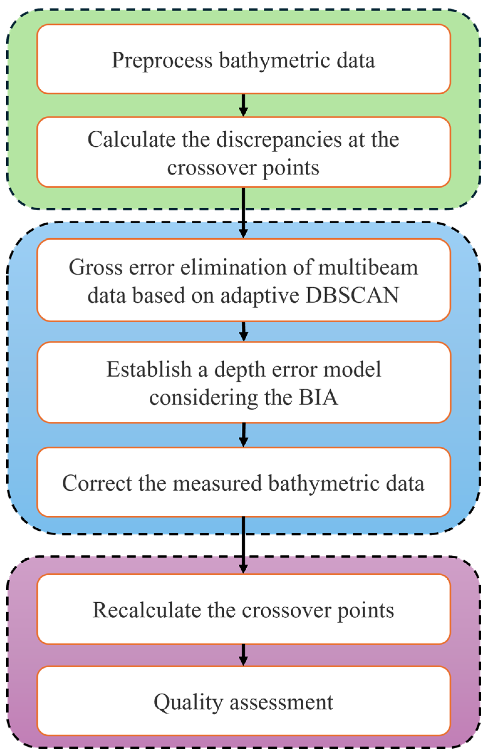
3.2. Experimental Process

In order to better demonstrate the reliability of the method proposed in this paper, the commonly used depth quadratic surface correction model was taken as the control. The same bathymetric data were processed using two methods, and a quality assessment was conducted in accordance with the requirements of relevant measurement specifications. The specific experimental steps were as follows, with the flowchart shown in Figure 4:

(1)

The preprocessing of depth measurement data: In the experiment, data processing such as draft correction, attitude correction, and water level correction was first carried out on the sounding data. Due to the influence of noise, the multibeam sounding data would contain obvious gross errors. Before fusing with high-precision sounding data, these gross errors had to be eliminated. Otherwise, the multibeam sounding data with gross errors being brought into the fused data model would have had a serious impact on the calculation.

(2)

Calculating the difference at the crossover of multibeam data: The 2022 edition of the Chinese National Standard for Hydrographic Surveys specification stipulates that depths within 1.0 mm between two points on a map are overlapping depths, while other parameters are not specified. Therefore, in this paper, the positions of each measurement point on the main measurement line were directly selected. This method can avoid additional depth errors and position errors generated during the grid processing of multibeam data, which may affect the accuracy and credibility of the measurement data. In the practical process of deep-sea and far-sea measurement, the scale of the survey area is generally 1:100,000. Therefore, 100 m was selected as the evaluation index for the same position. It is considered that two depths within 100 m belong to the same position and should participate in the comparison of the difference at crossover points.

(3)

Eliminating gross errors from multibeam data based on the proposed adaptive DBSCAN: We processed the crossover points data in accordance with the methods in Section 2.1 and set the parameters Eps and MinPts reasonably. Then, the data after the elimination of gross errors were compared with the data before the elimination of gross errors to test the effect of eliminating gross errors.

(4)

Establishing the depth error model considering the BIA: Using information such as the crossover point position, depth, and BIA obtained through screening, a bathymetric data correction model was established and the parameters of the characteristic equation were solved using the multiple linear regression method.

(5)

Correcting bathymetric data: The depth correction model based on incident angle compensation in Section 2.3 was utilized to correct the low-precision multibeam bathymetric data.

(6)

Assessing data quality: The data for the crossover point difference before correction and the data for the crossover point difference after correction were statistically analyzed. The traditional method of fitting the conic surface to correct the depth was taken as the control group result, and the number of points with the crossover point difference exceeding the limit out of the total number of points was determined. The 2022 edition of the Chinese National Standard for Hydrographic Surveys specification stipulates that the number of points with an over-limit cross-point difference should not exceed 10% of the total points. The requirements for cross-point differences are listed in

Table 3. The 2022 edition of the Chinese National Standard for Hydrographic Surveys specification stipulates the limit difference for crossover point difference values.

The Range of Depth Z (m)	The Limit Difference in the Crossover Depth Difference Values (m)
0–20	±0.5
20–30	±0.6
30–50	±0.7
50–100	±1.5
>100	±Z × 3%

. Further, the accuracy of multibeam data was measured based on the average value, standard deviation, maximum value, and minimum value of the crossover point difference.

3.3. AI-Assisted Language Polishing

In order to clearly express the content of this article and better correct grammatical errors, we used DeepSeek-R1 (https://www.deepseek.com (accessed on 1–2 June 2025)) to optimize the English grammar and expression of the first draft of the article. The results have been carefully reviewed and revised by the authors. The tool contributed only to syntactic improvements, with zero impact on scientific content or conclusions.

4. Results and Discussion

4.1. Adaptive DBSCAN Parameter Determination and Cluster Analysis

The quality inspection results for the crossover point difference in depth measurement are divided into over-limit data and non-over-limit data. For these two types of data, two different error correction methods are used for processing. The traditional quadratic surface error model was used as the reference group method and compared, through analysis, with the data results processed using the method proposed in this paper. The experimental results are given in this section.

In order to further improve the quality of the sounding results, the depth error correction model proposed in this paper was utilized to correct the errors for the obtained depths. According to the experimental steps in Section 3, the depth of the central beam of the inspection line and all the depths of the main measurement line were selected for the comparison of the crossover points differences. Firstly, the obtained bathymetric data were preprocessed and the processed bathymetric data were evaluated for the crossover points. The proposed adaptive DBSCAN algorithm was used to eliminate the gross differences in the crossover point differences. According to the data distribution of the crossover points, in order to better remove the edge error and retain the valid data as much as possible, 6102 data were employed in the comparison. According to the selection principle of MinPts, 2% of the total data size was taken as the experimental parameter in this paper, and the value of MinPts was set to 120. The value of eps was obtained through the inflection point of the k-distance curve graph, as shown in Figure 5.

By analyzing the k-distance curve in Figure 5, we can obtain the inflection point of the curve using the moving-window average method. It can be determined that the inflection point of this curve is 0.67. Therefore, 0.67 is taken as the value of the Eps parameter for the adaptive DBSCAN cluster analysis. The analysis results are shown in Figure 6.

The crossover points differences in the original data are distributed within the range of −150 m to 150 m. Among them, the data in the near-field area of 0–20 m are sparse and the distribution characteristics are not obvious. As the observation distance extends to 20–100 m, the number of data keeps increasing, the difference at the crossover points keeps increasing, and the overall distribution shows a divergent trend with the increase in distance. After processing using the proposed adaptive DBSCAN algorithm, the difference in the full-distance segment converges to the range of ±50 m, within which the difference in the 0–20 m area is reduced to ±20 m. At an observation distance of 80 m, the positive and negative error bands present symmetrical distribution characteristics, from −40 m to +40 m, conforming to the Gaussian distribution law. The error data at the edges have been effectively cleared, and most of the valid data have been retained. This reduces the influence of the error data on the measurement results without affecting surveyors’ perception of the seabed topography and geomorphology. The t-test was conducted on the data before and after correction. At the significance level α = 0.05, the t-test value was p = 0.00, which was less than the significance level α. Therefore, there was a significant difference before and after data cleaning. The effectiveness of the algorithm in rough error elimination and error equalization has been verified.

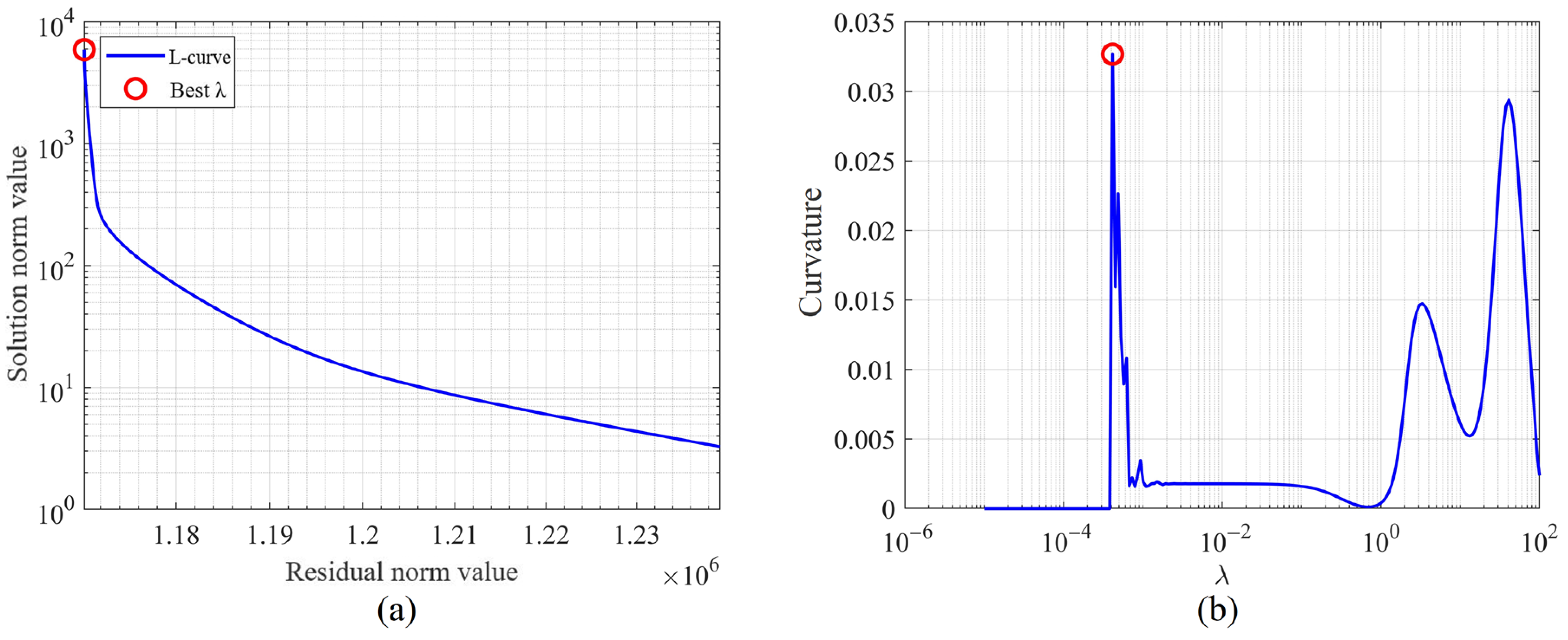
4.2. Determination of Regularization Parameters

In this study, the L-curve method is used to determine the size of the regularization parameter, and the calculation results are shown in Figure 7.

In the curvature variation graph of the L-curve in Figure 7b, the red dot is the point at which the curvature of the L-curve changes to the greatest extent, and its value is 4.15 $\times$ 10⁻⁴. This value is the λ value obtained from the L-curve. Substituting into Equation (17), the solution to the ill-weighted total least-squares problem can be obtained.

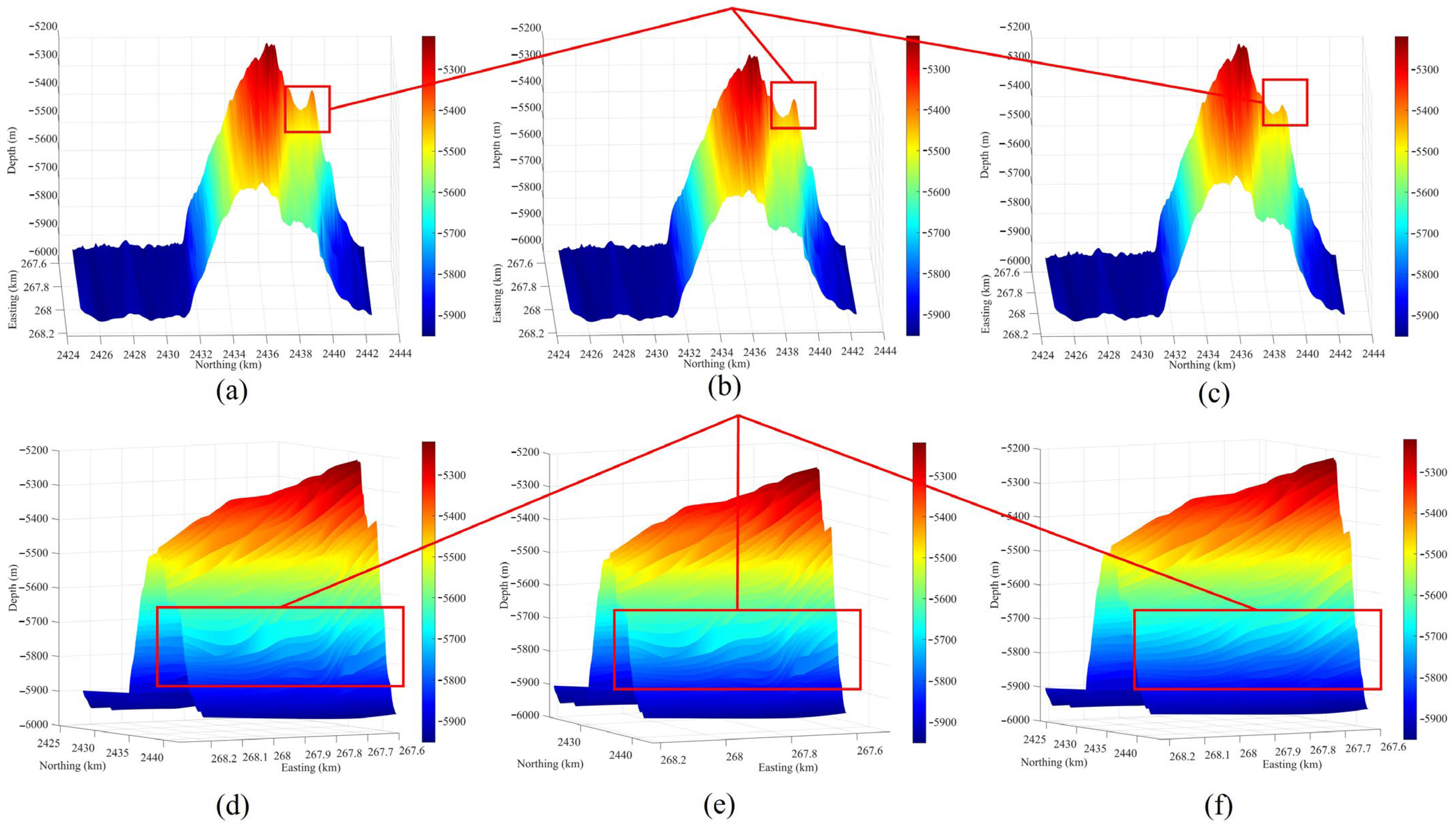
4.3. Comparison of the Correction Effects of the Depth Error Model

The method described in [36] is described as Method 1, and the method proposed in this paper is described as Method 2. Different methods were used to correct the bathymetric data, and the correction results are shown in

Table 4. Error comparison before and after bathymetric data correction.

Method	ME (m)			RMSE (m)			MAE (m)
	Z01	Z02	Z03	Z01	Z02	Z03	Z01	Z02	Z03
Original data	3.76	2.54	−2.58	16.21	19.64	24.18	118.61	127.62	146.77
Method 1	0	0	0	15.89	18.52	21.96	109.35	118.26	128.66
Method 2	0	0	0	10.77	14.15	16.95	48.61	50.09	69.91

.

In Table 4, the ME values of the original data at the crossover points formed by Z01, Z02, and Z03 and the inspection line are 3.76 m, 2.54 m, and −2.58 m, respectively, indicating that the survey vessel is greatly affected by the marine environment during the measurement process, and different survey lines contain different systematic errors. After correction via Methods 1 and 2, the ME values decreased significantly, indicating that both the traditional method and the method proposed in this paper can effectively eliminate the systematic errors contained in the measurement lines. However, in terms of the RMSE and MAE, there are significant differences in the correction effects of the two methods. The RMSE values of the crossover point statistics results of the corrected water depth data using Method 1 in the three different regions of Z01, Z02, and Z03 decreased by 1.9%, 5.7%, and 9.2%, respectively, and decreased by an average of 5.6% throughout the entire survey area. The RMSE of the crossover point statistics results of the water depth data corrected using Method 2 decreased by 33.6%, 28.0%, and 29.9%, respectively, in the three regions of Z01, Z02, and Z03 and decreased by an average of 30.4% throughout the entire survey area. The depth data corrected via Method 1 show some reductions in the RMSE and MAE, but the effect is not obvious. However, the depth data corrected via Method 2 show a significant reduction in the RMSE compared to the original data, effectively reducing the influence of outliers in the data. From the perspective of changes in the MAE, the correction effect of Method 1 is not ideal, with an average improvement of only 9.2%, while Method 2 has an average improvement of 57% in the survey area. A 4% reduction narrowed the error range of the measurement area from 150 m to 50 m, effectively improving the quality of the measured water depth data.

Comparing the error corrections of the method proposed in this paper under different water depths and error conditions illustrates the stable performance of the method under different terrain conditions, showing that it adapts to the complex seabed terrain area. Compared with the traditional correction methods, the method proposed in this paper has a more obvious and better effect on error correction.

Therefore, the conventional quadratic surface method solves the systematic deviation, but is ineffective regarding discreteness and outliers. The method proposed in this paper not only solves systematic deviation but also significantly improves the stability of the data. To further prove the effectiveness of the method proposed in this paper, the multibeam bathymetric data corrected using different methods were fitted into three-dimensional bathymetric topographic maps. The results are shown in Figure 8.

Through the analysis of the processed seabed topographic map, it can be deduced that the effect of the traditional method after correction is limited and some anomaly points are retained. The seabed topography corrected using the method in this paper is more realistic and reliable. It can be deduced from Figure 8a–c that for the abnormal data at the same position, the correction effect of the traditional method is not good and fails to effectively weaken the influence of outliers on the seabed topography. However, the abnormal data for seabed topography have been effectively weakened via correction using the method in this paper. The seabed topography after correction is gentler and does not affect the size of the normal bathymetric value data. It ensures the authenticity and reliability of the topography and landforms of the seabed. It can be seen from Figure 8d–f that the original seabed topography presents large, folded seabed landforms. After being corrected using conventional methods, the folded changes in the seabed topography still exist and the correction effect is not ideal. After correction using the method in this paper, it can be clearly seen from the red box area in Figure 8f that the changing trend in the seabed topography is gentler and the trend is more in line with the shape of the natural topography. The abnormal data for folds in the seabed topography are effectively eliminated, conforming to the structural characteristics of the general seabed topography and landforms and enhancing the current situation and data quality of the seabed topography data.

To summarize, compared with the traditional quadratic bathymetric surface model, the method proposed in this paper is superior in terms of both the statistical results for the difference at the crossover points and the quality of the generated seabed topographic map. Moreover, data quality was further improved through correction using the method in this paper. The influence of the residual errors in the processing of measurement data on the bathymetric data was further weakened, and the credibility and quality of data were enhanced.

5. Conclusions

This study proposes a comprehensive framework to enhance MBES data quality in USV operations by introducing an innovative crossover error adjustment strategy. Three core methodological advances were validated through field experiments in the Western Pacific: the adaptive DBSCAN algorithm for robust outlier detection, an asymmetric quadratic surface model incorporating beam incidence angle (BIA) with dynamic weighting for improved edge beam correction, and a Tikhonov-regularized weighted least-squares solution for large-scale data stability. These enhancements yielded significant reductions in error metrics and improved topographic consistency, surpassing conventional methods. The proposed framework aligns with hydrographic standards and preserves seabed morphology.

Future work will focus on real-time deployment in dynamic marine environments, with an emphasis on integrating machine learning techniques to enable autonomous parameter optimization in USV systems.

References

1. Quiñones, J.D.P.; Sladen, A.; Ponte, A.; Lior, I.; Ampuero, J.-P.; Rivet, D.; Meulé, S.; Bouchette, F.; Pairaud, I.; Coyle, P. High Resolution Seafloor Thermometry for Internal Wave and Upwelling Monitoring Using Distributed Acoustic Sensing. Sci. Rep. 2023, 13, 17459. [Google Scholar] [CrossRef]
2. Loureiro, G.; Dias, A.; Almeida, J.; Martins, A.; Hong, S.; Silva, E. A Survey of Seafloor Characterization and Mapping Techniques. Remote Sens. 2024, 16, 1163. [Google Scholar] [CrossRef]
3. Shang, X.; Zhao, J.; Zhang, H. Obtaining High-Resolution Seabed Topography and Surface Details by Co-Registration of Side-Scan Sonar and Multibeam Echo Sounder Images. Remote Sens. 2019, 11, 1496. [Google Scholar] [CrossRef]
4. Ashphaq, M.; Srivastava, P.K.; Mitra, D. Review of Near-Shore Satellite Derived Bathymetry: Classification and Account of Five Decades of Coastal Bathymetry Research. J. Ocean. Eng. Sci. 2021, 6, 340–359. [Google Scholar] [CrossRef]
5. Sun, H.; Li, Q.; Bao, L.; Wu, Z.; Wu, L. Progress and Development Trend of Global Refined Seafloor Topography Modeling. Geomat. Inf. Sci. Wuhan Univ. 2022, 47, 1555–1567. [Google Scholar] [CrossRef]
6. Janowski, Ł.; Tęgowski, J.; Montereale-Gavazzi, G. Editorial: Seafloor Mapping Using Underwater Remote Sensing Approaches. Front. Earth Sci. 2023, 11, 1306202. [Google Scholar] [CrossRef]
7. Yu, X.; Wang, J.; Cui, Y. An Algorithm for Sound Velocity Error Correction Using GA-SVR Considering the Distortion Characteristics of Seabed Topography Measured by Multibeam Sonar Mounted on Autonomous Underwater Vehicle. IEEE J. Sel. Top. Appl. Earth Obs. Remote Sens. 2024, 17, 20209–20226. [Google Scholar] [CrossRef]
8. Grządziel, A. Method of Time Estimation for the Bathymetric Surveys Conducted with a Multi-Beam Echosounder System. Appl. Sci. 2023, 13, 10139. [Google Scholar] [CrossRef]
9. Cao, W.; Fang, S.; Zhu, C.; Feng, M.; Zhou, Y.; Cao, H. Three-Dimensional Non-Uniform Sampled Data Visualization from Multibeam Echosounder Systems for Underwater Imaging and Environmental Monitoring. Remote Sens. 2025, 17, 294. [Google Scholar] [CrossRef]
10. Sotelo-Torres, F.; Alvarez, L.V.; Roberts, R.C. An Unmanned Surface Vehicle (USV): Development of an Autonomous Boat with a Sensor Integration System for Bathymetric Surveys. Sensors 2023, 23, 4420. [Google Scholar] [CrossRef]
11. Wang, L.; Zhu, D.; Pang, W.; Zhang, Y. A Survey of Underwater Search for Multi-Target Using Multi-AUV: Task Allocation, Path Planning, and Formation Control. Ocean Eng. 2023, 278, 114393. [Google Scholar] [CrossRef]
12. Wang, J.; Tang, Y.; Jin, S.; Bian, G.; Zhao, X.; Peng, C. A Method for Multi-Beam Bathymetric Surveys in Unfamiliar Waters Based on the AUV Constant-Depth Mode. J. Ocean. Eng. Sci. 2023, 11, 1466. [Google Scholar] [CrossRef]
13. Lubczonek, J.; Kazimierski, W.; Zaniewicz, G.; Lacka, M. Methodology for Combining Data Acquired by Unmanned Surface and Aerial Vehicles to Create Digital Bathymetric Models in Shallow and Ultra-Shallow Waters. Remote Sens. 2022, 14, 105. [Google Scholar] [CrossRef]
14. Makar, A. Determination of the Minimum Safe Distance between a USV and a Hydro-Engineering Structure in a Restricted Water Region Sounding. Energies 2022, 15, 2441. [Google Scholar] [CrossRef]
15. Yang, F.; Li, J.; Han, L.; Liu, Z. The Filtering and Compressing of Outer Beams to Multibeam Bathymetric Data. Mar. Geophys. Res. 2013, 34, 17–24. [Google Scholar] [CrossRef]
16. Rezvani, M.-H.; Sabbagh, A.; Ardalan, A.A. Robust Automatic Reduction of Multibeam Bathymetric Data Based on M-Estimators. Mar. Geod. 2015, 38, 327–344. [Google Scholar] [CrossRef]
17. Ferreira, I.O.; Santos, A.D.P.D.; Oliveira, J.C.D.; Medeiros, N.D.G.; Emiliano, P.C. Spatial outliers detection algorithm (soda) applied to multibeam bathymetric data processing. Bol. Ciênc. Geod. 2019, 25, e2019020. [Google Scholar] [CrossRef]
18. He, G.; Gao, X.; Li, L.; Gao, P. OCT Monitoring Data Processing Method of Laser Deep Penetration Welding Based on HDBSCAN. Opt. Laser Technol. 2024, 179, 111303. [Google Scholar] [CrossRef]
19. Nasaruddin, N.; Masseran, N.; Idris, W.M.R.; Ul-Saufie, A.Z. A SMOTE PCA HDBSCAN Approach for Enhancing Water Quality Classification in Imbalanced Datasets. Sci. Rep. 2025, 15, 13059. [Google Scholar] [CrossRef]
20. Li, M.; Sun, L.; Sun, Q.; Jin, S. Adjustment Model Based on Ping Sructure for Swath Combination Net. Geomat. Inf. Sci. Wuhan Univ. 2011, 36, 652–655. [Google Scholar] [CrossRef]
21. Huang, C.; Lu, X.; Liu, S.; Bian, G.; Ouyang, Y.; Huang, X.; Deng, K. Examination and Assessment of Bathymetric Surveying Products, Part I: Design of Cross Point Discrepancy Array. Hydrogr. Surv. Charting 2017, 37, 11–16. [Google Scholar]
22. Xu, Y.; Gao, A.; Sun, L.; Lv, Y. Adjusting the Sounding Data’s System Error Acquired in a Grid Pattern. Eng. Surv. Mapp. 2016, 25, 21–24+29. [Google Scholar] [CrossRef]
23. Jakobsson, M.; Calder, B.; Mayer, L. On the Effect of Random Errors in Gridded Bathymetric Compilations. J. Geophys. Res.-Solid Earth 2002, 107, ETG 14-1–ETG 14-11. [Google Scholar] [CrossRef]
24. Yang, F.; Li, J.; Liu, Z.; Han, L. Correction for Depth Biases to Shallow Water Multibeam Bathymetric Data. China Ocean Eng. 2013, 27, 245–254. [Google Scholar] [CrossRef]
25. Plant, N.G.; Holland, K.T.; Puleo, J.A. Analysis of the Scale of Errors in Nearshore Bathymetric Data. Mar. Geol. 2002, 191, 71–86. [Google Scholar] [CrossRef]
26. Liu, Y.; Wu, Z.; Zhao, D.; Zhou, J.; Shang, J.; Wang, M.; Zhu, C.; Lu, H. The MF Method for Multi-Source Bathymetric Data Fusion and Ocean Bathymetric Model Construction. Acta Geod. Cartogr. Sin. 2019, 48, 1171–1181. [Google Scholar]
27. Guo, Y.; Zocca, S.; Dabove, P.; Dovis, F. A Post-Processing Multipath/NLoS Bias Estimation Method Based on DBSCAN. Sensors 2024, 24, 2611. [Google Scholar] [CrossRef]
28. Mehmood, Z.; Wang, Z. Hybrid iForest-DBSCAN for Anomaly Detection and Wind Power Curve Modelling. Expert. Syst. Appl. 2025, 289, 128381. [Google Scholar] [CrossRef]
29. Han, J.; Guo, X.; Jiao, R.; Nan, Y.; Yang, H.; Ni, X.; Zhao, D.; Wang, S.; Ma, X.; Yan, C.; et al. An Automatic Method for Delimiting Deformation Area in InSAR Based on HNSW-DBSCAN Clustering Algorithm. Remote Sens. 2023, 15, 4287. [Google Scholar] [CrossRef]
30. Li, Y.; Wang, J.; Zhao, H.; Wang, C.; Shao, Q. Adaptive DBSCAN Clustering and GASA Optimization for Underdetermined Mixing Matrix Estimation in Fault Diagnosis of Reciprocating Compressors. Sensors 2023, 24, 167. [Google Scholar] [CrossRef]
31. Frankl, N.; Kupavskii, A. Nearly K-Distance Sets. Discrete. Comput. Geom. 2023, 70, 455–494. [Google Scholar] [CrossRef]
32. Dirgantoro, G.P.; Soeleman, M.A.; Supriyanto, C. Smoothing Weight Distance to Solve Euclidean Distance Measurement Problems in K-Nearest Neighbor Algorithm. In Proceedings of the 2021 IEEE 5th International Conference on Information Technology, Information Systems and Electrical Engineering (ICITISEE), Purwokerto, Indonesia, 24–25 November 2021; pp. 294–298. [Google Scholar]
33. Agarwal, A.; Kakade, S.M.; Lee, J.D.; Mahajan, G. On the Theory of Policy Gradient Methods: Optimality, Approximation, and Distribution Shift. J. Mach. Learn. Res. 2021, 22, 1–76. [Google Scholar]
34. Alikhanov, A.A.; Asl, M.S.; Huang, C. Stability Analysis of a Second-Order Difference Scheme for the Time-Fractional Mixed Sub-Diffusion and Diffusion-Wave Equation. Fract. Calc. Appl. Anal. 2024, 27, 102–123. [Google Scholar] [CrossRef]
35. Mokhtari, F.; Akhlaghi, M.I.; Simpson, S.L.; Wu, G.; Laurienti, P.J. Sliding Window Correlation Analysis: Modulating Window Shape for Dynamic Brain Connectivity in Resting State. NeuroImage 2019, 189, 655–666. [Google Scholar] [CrossRef] [PubMed]
36. Luo, J. The Processing M ethod of M ulti-beam and Single-beam Bathymetric Data Fusion. Hydrogr. Surv. Charting 2018, 38, 21–24. [Google Scholar]
37. Marjetič, A.; Ambrožič, T.; Savšek, S. Use of Total Least Squares Adjustment in Geodetic Applications. Appl. Sci. 2024, 14, 2516. [Google Scholar] [CrossRef]
38. Vestøl, O.; Breili, K.; Taskjelle, T. Common Adjustment of Geoid and Mean Sea Level with Least Squares Collocation. J. Geod. 2025, 99, 40. [Google Scholar] [CrossRef]
39. Li, Z.; Peng, Z.; Zhang, Z.; Chu, Y.; Xu, C.; Yao, S.; García-Fernández, Á.F.; Zhu, X.; Yue, Y.; Levers, A.; et al. Exploring Modern Bathymetry: A Comprehensive Review of Data Acquisition Devices, Model Accuracy, and Interpolation Techniques for Enhanced Underwater Mapping. Front. Mar. Sci. 2023, 10, 1178845. [Google Scholar] [CrossRef]
40. Lurton, X. An Introduction to Underwater Acoustics: Principles and Applications, 2nd ed.; Springer: Berlin, Germany, 2010; Chapter 7.2; pp. 235–238. [Google Scholar]
41. Xu, T.; Yang, Y. Robust Tikhonov Regularization Method and Its Applications. Geomat. Inf. Sci. Wuhan Univ. 2003, 28, 719–722. [Google Scholar]
42. Fischer, A.; Cellmer, S.; Nowel, K. Assessment of the Double-Parameter Iterative Tikhonov Regularization for Single-Epoch Measurement Model-Based Precise GNSS Positioning. Measurement 2023, 218, 113251. [Google Scholar] [CrossRef]
43. Li, M.; Wang, L.; Luo, C.; Wu, H. A New Improved Fractional Tikhonov Regularization Method for Moving Force Identification. Structures 2024, 60, 105840. [Google Scholar] [CrossRef]
44. Gerth, D. A New Interpretation of (Tikhonov) Regularization. Inverse Probl. 2021, 37, 064002. [Google Scholar] [CrossRef]
45. Du, W.; Zhang, Y. The Calculation of High-Order Vertical Derivative in Gravity Field by Tikhonov Regularization Iterative Method. Math. Probl. Eng. 2021, 2021, 8818552. [Google Scholar] [CrossRef]
46. Xing, J.; Chen, X.-X.; Ma, L. Bathymetry Inversion Using the Modified Gravity-Geologic Method: Application of the Rectangular Prism Model and Tikhonov Regularization. Appl. Geophys. 2020, 17, 377–389. [Google Scholar] [CrossRef]
47. Li, X.; Xiong, Y.; Xu, S.; Chen, W.; Zhao, B.; Zhang, R. A Multipath Error Reduction Method for BDS Using Tikhonov Regularization with Parameter Optimization. Remote Sens. 2023, 15, 3400. [Google Scholar] [CrossRef]
48. Calvetti, D.; Morigi, S.; Reichel, L.; Sgallari, F. Tikhonov Regularization and the L-curve for Large Discrete Ill-Posed Problems. J. Comput. Appl. Math. 2000, 123, 423–446. [Google Scholar] [CrossRef]
49. Maharani, M.; Saputro, D.R.S. Generalized Cross Validation (GCV) in Smoothing Spline Nonparametric Regression Models. J. Phys. Conf. Ser. 2021, 1808, 012053. [Google Scholar] [CrossRef]
50. Wang, L.; Xu, C.; Lu, T. Ridge Estimation Method in Ill-posed Weighted Total Least Squares Adjustment. Geomat. Inf. Sci. Wuhan Univ. 2010, 35, 1346–1350. [Google Scholar] [CrossRef]
51. Tong, H. Functional Linear Regression with Huber Loss. J. Complex. 2023, 74, 101696. [Google Scholar] [CrossRef]
Figure 1. Spatial distribution characteristics of crossover points differences.
Jmse 13 01364 g001
Figure 2. Distribution diagram showing the relationship between the crossover point difference and the BIA.
Jmse 13 01364 g002
Figure 3. Schematic diagram of the survey area. The area in the red box is the area for calculating the difference at the crossover points.
Jmse 13 01364 g003
Figure 4. Flowchart of experimental steps. The green background area indicates the data preparation stage. The blue background area indicates the data correction stage. The purple background area indicates the data quality assessment stage.
Jmse 13 01364 g004
Figure 5. The k-distance curve for the crossover point difference in multibeam data.
Jmse 13 01364 g005
Figure 6. Comparison of the distribution of crossover point differences before and after eliminating gross errors from multibeam data. The yellow dot-shaped symbols represent the valid data after DBSCAN clustering, and the red cross-shaped symbols represent the noisy data.
Jmse 13 01364 g006
Figure 7. Determination of regularization parameters. (a) The L-curve variation graph; (b) the curvature variation graph for the L-curve. The position marked with the red circle has the greatest curvature variation, and the corresponding value is the optimal parameter value.
Jmse 13 01364 g007
Figure 8. Comparison of seabed topographic map composed of multibeam bathymetric data before and after error correction. (a,d) Original three-dimensional maps of the seabed topography. (b,e) Three-dimensional seabed topographic maps corrected using the traditional quadratic surface model. (c,f) Three-dimensional seabed topographic maps corrected using the method proposed in this paper. The red box indicates the areas where the seabed topography has distinct features before and after correction.
Jmse 13 01364 g008