Classification of Underwater Sediments in Lab Based on LiDAR Full-Waveform Data

Abstract

The classification of shallow sea sediments based on airborne LiDAR bathymetry represents a significant advancement in marine science and engineering. Airborne LiDAR is a highly valuable tool for the classification of seabed sediments, offering high accuracy and mobility. However, accurately classifying shallow marine sediments remains a challenging endeavor due to the difficulties associated with differentiation and the inherent limitations in accuracy. To achieve the accurate classification of underwater sediments, a feature selection method for underwater sediment classification is proposed in this paper and tested in a laboratory environment. The method inputs the original feature set into a classification algorithm that combines Sequential Forward Selection with Random Forests. The study demonstrates that the model achieves an overall classification accuracy of 94.1% and a Kappa coefficient of 91.11%, thereby enabling the accurate and efficient classification of underwater sediment. This approach can be employed as a supplementary technique for the precise classification of shallow marine sediments, offering valuable assistance in the examination of marine ecosystems.

1. Introduction

Seabed sediments provide crucial information for analyzing the marine environment, biological habitats, and geological features. The classification of shallow sea sediments is of great significance, providing fundamental data and decision-making support for the development of marine resources, ecological protection, and marine scientific research.

Currently, seabed sediment classification methods are typically divided into two categories: field sampling and remote sensing detection [1]. In the context of field sampling, direct observation and the collection of seabed sediment samples are conducted using a range of tools, including samplers, manned submersibles, and remotely operated vehicles (ROVs) [2]. In seafloor sediment classification studies, the method provides high-precision information on seafloor sediments. However, it is limited in its application due to its high economic cost and low sampling efficiency. These limitations make it difficult for the method to meet the needs of application scenarios such as a single short survey missions, wide area coverage, and the sediment detection of unknown seafloor areas. Remote sensing detection has been widely used in related research to achieve seabed sediment classification [3]. The most representative methods are acoustic remote sensing detection [4] and optical remote sensing detection. Acoustic remote sensing employs a range of instruments, including side-scan sonar, multibeam systems [5,6], and sonic topographers, to detect seabed sediment. The propagation and reflection characteristics of acoustic waves are used to obtain information about the sediment, and the characteristics of the received acoustic signals are used to classify it [3,7,8]. For example, the transmission time of sound waves from the surface of the water to the bottom and back to the surface is slower than that of light waves. Furthermore, the transmission of sound pulses in the acoustic remote sensing detection technique is limited by the speed of sound in the water. It is therefore important to ensure that the speed of the vessel carrying the sound pulses is not too fast. When both optical and acoustic remote sensing detection techniques are employed to detect the same depth of water, the acoustic remote sensing detection technique exhibits a slight reduction in efficiency. Moreover, in shallow water and shallow terrain, the deployment of acoustic remote sensing detection equipment on a vessel is necessary, though such vessels are susceptible to stranding and present a hazard. Furthermore, lateral multibeam acoustic transmissions may be impeded by the presence of reefs, thereby reducing the detection range and precluding the inclusion of any land in the route planning. These constraints render the attainment of highly precise outcomes for the classification of shallow seabed sediments a challenging endeavor. The application of optical remote sensing detection in shallow sea environments is limited by several factors, which include errors in time or distance estimation; refraction effects; turbidity; wave breaking; biota interference; and light conditions. In order to enhance its applicability and reliability in such complex environments, methods such as multi-source data fusion and environmental correction algorithms are required.

Optical remote sensing detection, as represented by airborne lidar bathymetry, is an active optical remote sensing method which provides high accuracy for the detection of shallow sea areas. It demonstrates remarkable flexibility and efficiency with regard to spatial coverage, mission execution, and data acquisition [9]. In recent years, various scholars [10,11,12] have conducted research and implemented updates to the airborne bathymetric LiDAR system, which is now widely utilized in the fields of hydrological geomorphology, water conservancy engineering, and other related disciplines. The depth performance, accuracy, and other key indicators of this system have been enhanced to a notable extent. As demonstrated in

Table 1. LiDAR systems and depth performance.

LiDAR System	Affiliations and Addresses	Depth Performance
VQ-820-G	RIEGL Laser Measurement Systems GmbH; Riedenburgstraße 48, A-3580 Horn, Austria	1 Secchi depth
TDOT3	Geo Drone Solutions; Brisbane, Queensland, Australia	1.4 Secchi depth (reflectance of 1.0, absorption coefficient of 0.25), 1.25 times depth of Secchi disk (reflectance of 0.5, absorption coefficient of 0.25), and 1 times Secchi disk (reflectance of 0.2, absorption coefficient of 0.25)
VQ-880-G	RIEGL Laser Measurement Systems GmbH; Riedenburgstraße 48, A-3580 Horn, Austria	1.5 Secchi depth
VQ-880-G II	RIEGL Laser Measurement Systems GmbH; Riedenburgstraße 48, A-3580 Horn, Austria	1.5 Secchi depth
Mapper-20kU	Shanghai Institute of Optics and Fine Mechanics; Shanghai, China	1.5 Secchi depth
Photon counting LiDAR	Key Laboratory of Geological Survey and Evaluation of Ministry of Education, China University of Geosciences (Wuhan); Wuhan, China	2 Secchi depth
VQ-840-G	RIEGL Laser Measurement Systems GmbH; Riedenburgstraße 48, A-3580 Horn, Austria	1.7, 1.8, 2.0, 2.2, and 2.5 Secchi depth (measurement rate of 200, 100, 50, 5, and 0.5 kHz, respectively)

, the LiDAR system and its depth performance are presented. Studies have demonstrated that airborne LiDAR systems can explore shallow sea areas, and the LiDAR full-waveform and topographic features obtained from the data can aid in understanding the type, composition, and distribution of shallow sea sediments [13,14,15,16]. In particular, the analysis of full-waveform data from LiDAR systems is of significant importance for the classification and identification of shallow marine sediments [17].

Several studies have been conducted on the classification of seabed sediment using optical data, both in China and abroad. Velasco et al. [18] proposed a method that employs a streamlined radiative transfer model and cluster analysis to process backscattered intensity and depth data. The researchers were able to successfully classify the seabed sediment into 15 distinct categories. Kumpumäki et al. [17] demonstrated that waveform characteristics can accurately describe seabed sediment types in the study area. They achieved this by modeling return pulse waveforms and using self-organizing mapping for feature mapping and cluster analysis. Tissue mapping was used for feature mapping and cluster analysis to accurately describe the benthic cover types in the study area. The results showed that waveform features can be used to describe seabed sediment types. Eren et al. [19,20] observed a strong correlation between LiDAR waveform features and seabed sediment. Subsequently, a support vector machine was employed to categorize the samples as either sand or rock, and as belonging to the fine or coarse sand categories. The resulting accuracy rates were 96% and 86%, respectively. Wilson et al. [21] proposed a set of waveform features based on the shape of EAARL-B as a basis for differentiating shallow sea bottom corals and their morphology. Amani et al. [22] classified five types of shallow sea sediments, including those containing gravel, fine seabed sediments, and macroalgae, with an 80% accuracy rate using LiDAR intensity imagery and a Random Forest algorithm. To summarize, the features of the waveform obtained from the airborne LiDAR system data are crucial for the classification of seabed sediment. The machine learning model demonstrates a high level of proficiency in identifying marine environments.

The integration of remote sensing data with physical samples is a valuable approach in the realm of geological and marine environmental research. Remote sensing technology is utilized to obtain large-scale, high-resolution spatial data and to combine it with on-site sampling to verify the classification results and to improve the accuracy and reliability of geological investigations [23,24]. This approach enhances the precision of seabed geological mapping and showcases the potential of data integration and machine learning in geological investigations. The utilization of this approach is pivotal in optimizing the value of data, fostering the advancement of geoscientific research, and providing scientific substantiation in domains such as resource exploration, ecological preservation, and environmental monitoring.

The objective of this study is to address the challenges of distinguishing between shallow sea sediments and achieving accurate seabed sediment classification.In order to achieve the high-precision classification of underwater sediments, the study utilizes seafloor optical data extracted by a LiDAR system under laboratory conditions to facilitate the identification of relevant features. Subsequently, the method of machine learning feature selection and classification is employed. The findings of this research have significant theoretical and practical implications for several fields, including shallow sea resource development, ecological protection, engineering applications, and shallow sea scientific research.

2. Background and Data

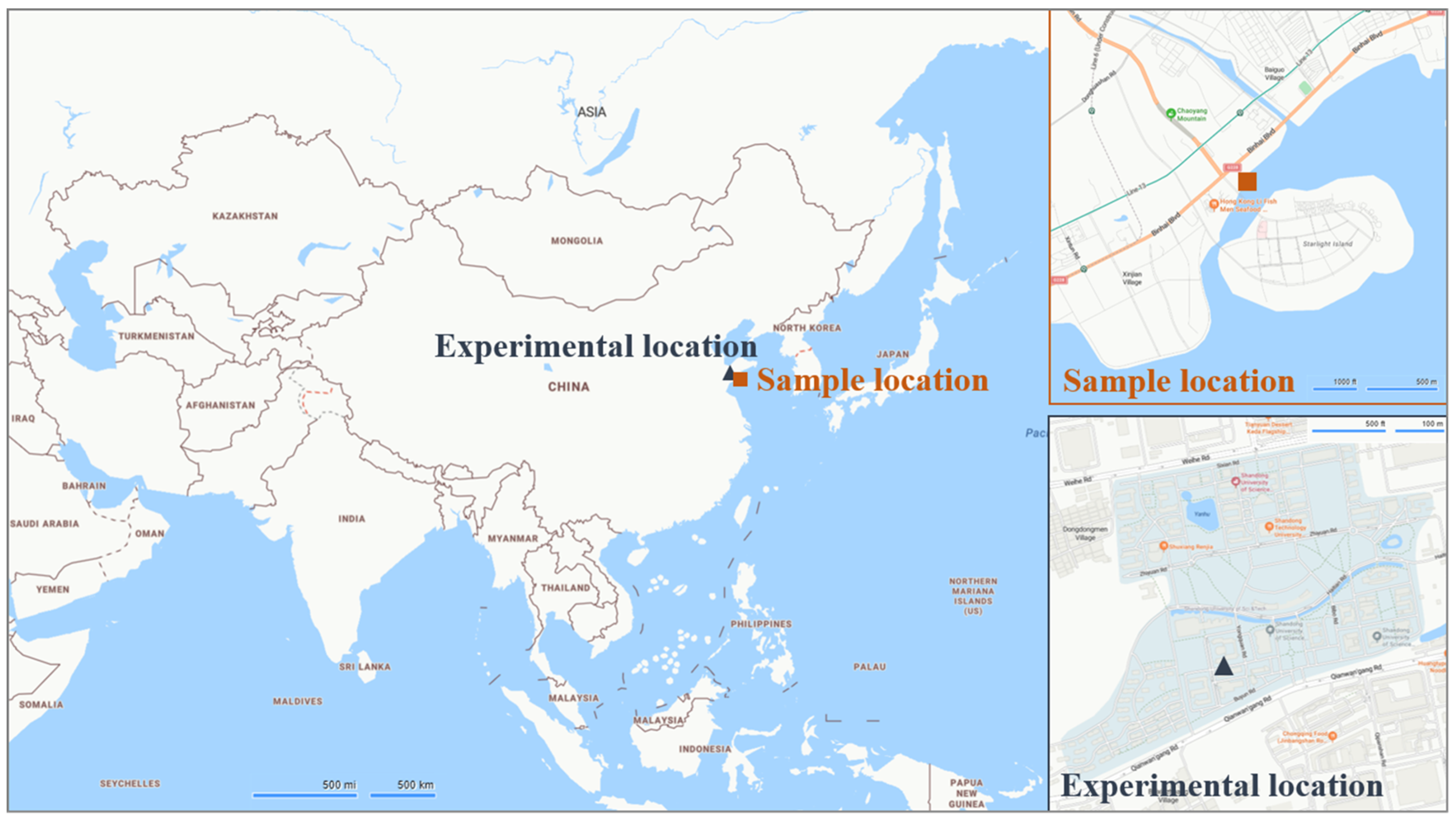
This paper presents an analysis of the shallow sea sediments of specific coastal areas in the Yellow Sea of China; this area is shown in Figure 1. The material of the sediment samples was examined at the sampling site, and four categories of samples were collected: these were, namely, sand (material between 0.0625 and 2 mm), mud (all material less than 0.0625 mm, i.e., chalk plus clay), gravel (material coarser than 2 mm), and rock (sand to mud ratio greater than 9:1, i.e., sandstone) [25], as illustrated in Figure 2.

The samples were collected according to classification criteria at the time of sampling. When setting up the scene in the laboratory, the samples of each category were placed at the same location for the same category, and at different locations for different categories and at long distances, to ensure that the content of the category of each sample was 85% or more at the LIDAR detection site, and that the target was identified as a single category (the criteria for identification of a single category were that the content of the category was >80%) [26], so as to ensure that the data corresponded to the category of the target and that they were not interfered with by the mixture of the target objects.

The sand in this study is composed of fine granular quartz, feldspar, and detritus. The mud comprises fine-grained clay and organic matter, exhibiting soft and wet characteristics. In comparison to gravel and rock, sand and mud have a rougher surface. The substrate surface’s roughness characteristics are a significant basis for classification. From the perspective of the detection system, the LiDAR system emits a laser light with a spot radius that is larger than the surface area of a single gravel particle. This allows the laser spot to cover multiple pieces of gravel. In contrast, the laser spot radius is smaller than the surface area of a single rock. The spot diameter of the LiDAR system utilized in the experiment is 1.5 cm; therefore, gravel and rock samples with a minimum side length of less than 1.5 cm were selected as the test gravels, while rock samples with a plane diameter exceeding 5 cm were employed as the test rocks.

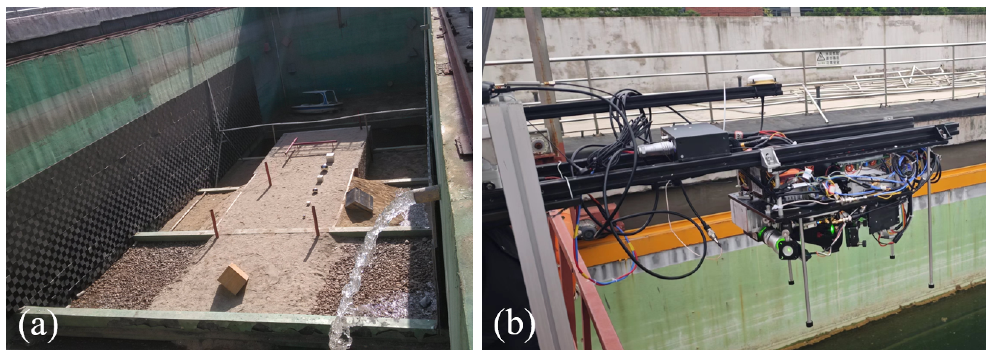
The sediment samples obtained from the field were situated within a partition of the experimental site at the Shandong University of Science and Technology as Figure 1. The test area exhibited a water depth range of 0.3–0.7 m, a low level of turbidity, a seafloor slope of 0°–0.5°, and an overall flat topography. The dimensions of the test field measured 40 m in length and 11 m in width, as shown in Figure 3a. The remaining conditions were maintained at a moderate level to emulate a genuine shallow marine environment. The LiDAR full-waveform data were obtained by measuring various types of seafloor texture present in the test area using the LiDAR system developed by the research team as Figure 3b [27]. The principal parameters are enumerated in

Table 2. Main parameters of the self-developed LiDAR system.

Parameter	Index
Laser wavelength	532 nm
Laser repetition frequency	5 kHz
Laser spot radius	1.5 cm
Bathymetric range	1.5 Seawater attenuation lengths
Position accuracy	Horizontal positioning accuracy: 0.01 m
	Elevation measurement accuracy: 0.05 m
Attitude accuracy	Pitch and roll angle measurement accuracy: 0.01°
	Heading angle measurement accuracy: 0.05°
Equipment weight	≤20 kg

.

The high resolution and sensitivity of LiDAR full-waveform data allow for the collection of detailed substrate characteristics, thereby conferring significant advantages in the classification of underwater sediments. A total of 2000 samples comprising 500 samples each of sand, mud, gravel, and rock types were utilized in the study. The sand, gravel, and rock samples were placed at a water depth of 0.7 m in the designated test area, while the mud samples were placed at a water depth of 0.3 m.

For parameter tuning and model evaluation, the dataset was divided into a training set and a test set using cross-validation with a 7:3 ratio. The training set is employed for the purpose of model development, while the test set is utilized for evaluation purposes.

3. Method

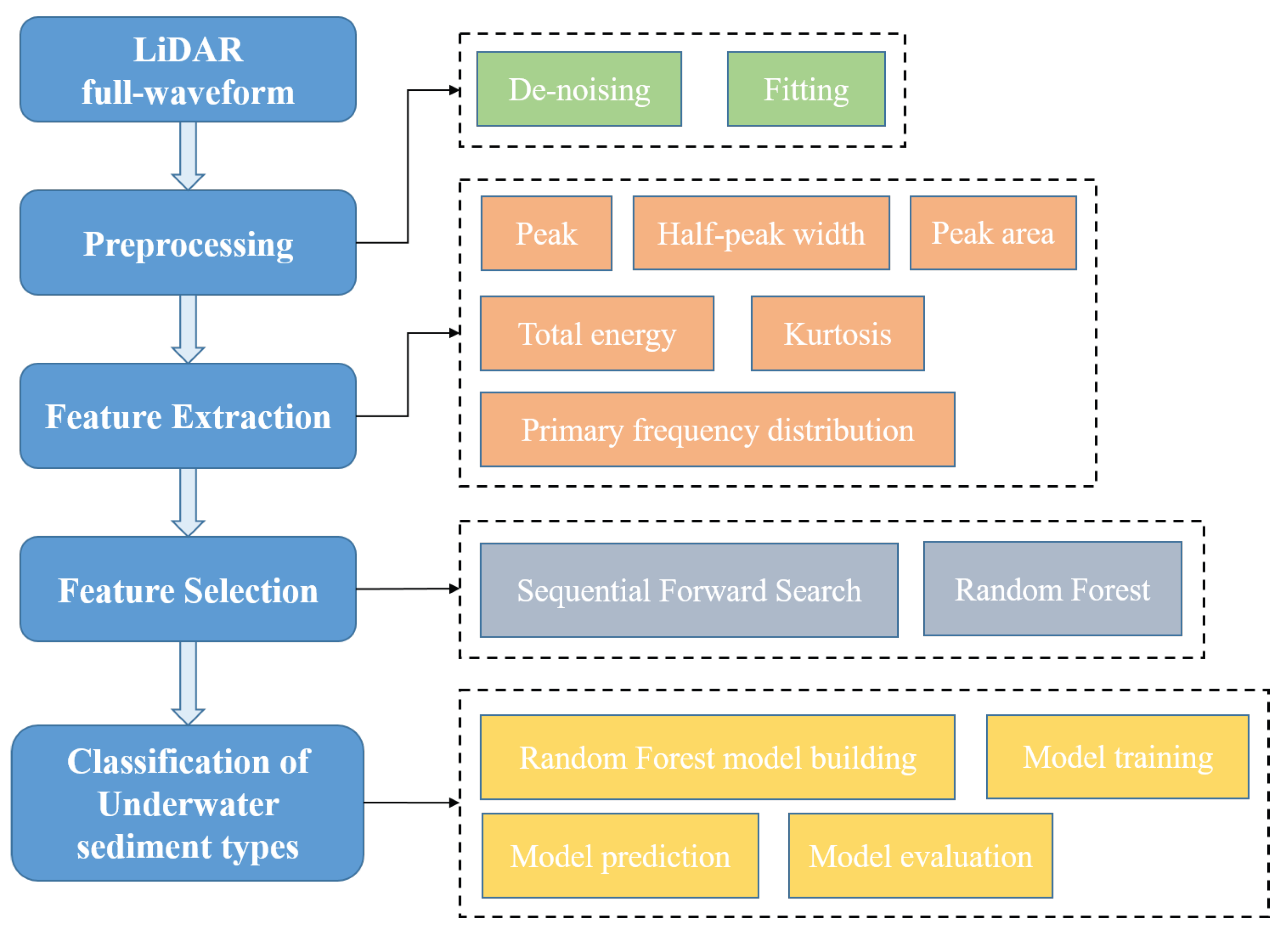
To tackle the issue of classifying shallow sea sediments, this study proposes a Random Forest approach for underwater sediment classification with feature selection. The method comprised the following steps, as illustrated in Figure 4: (1) Initially, the raw LiDAR full-waveform data are subjected to preprocessing to eliminate noise and ensure data compatibility. (2) Subsequently, the LiDAR full-waveform data are subjected to feature extraction, thereby generating the original feature set. (3) The original feature set is then augmented with the addition of selected features, which are identified through a combination of Sequential Forward Selection and Random Forest. (4) Ultimately, the Random Forest algorithm is employed for the classification of diverse types of underwater sedimentary data.

3.1. Preprocessing

The full-waveform data from the LiDAR system may be subject to contamination by a variety of noise sources when employed for the detection of submerged sedimentary deposits. Background noise, which gives rise to random intensity fluctuations in the full-waveform data, is constituted by atmospheric turbulence and particulate matter, multiple reflections of the laser beam during propagation, and refraction interference. In this study, background noise was removed from all laser full-waveform sample data to achieve effective feature extraction.

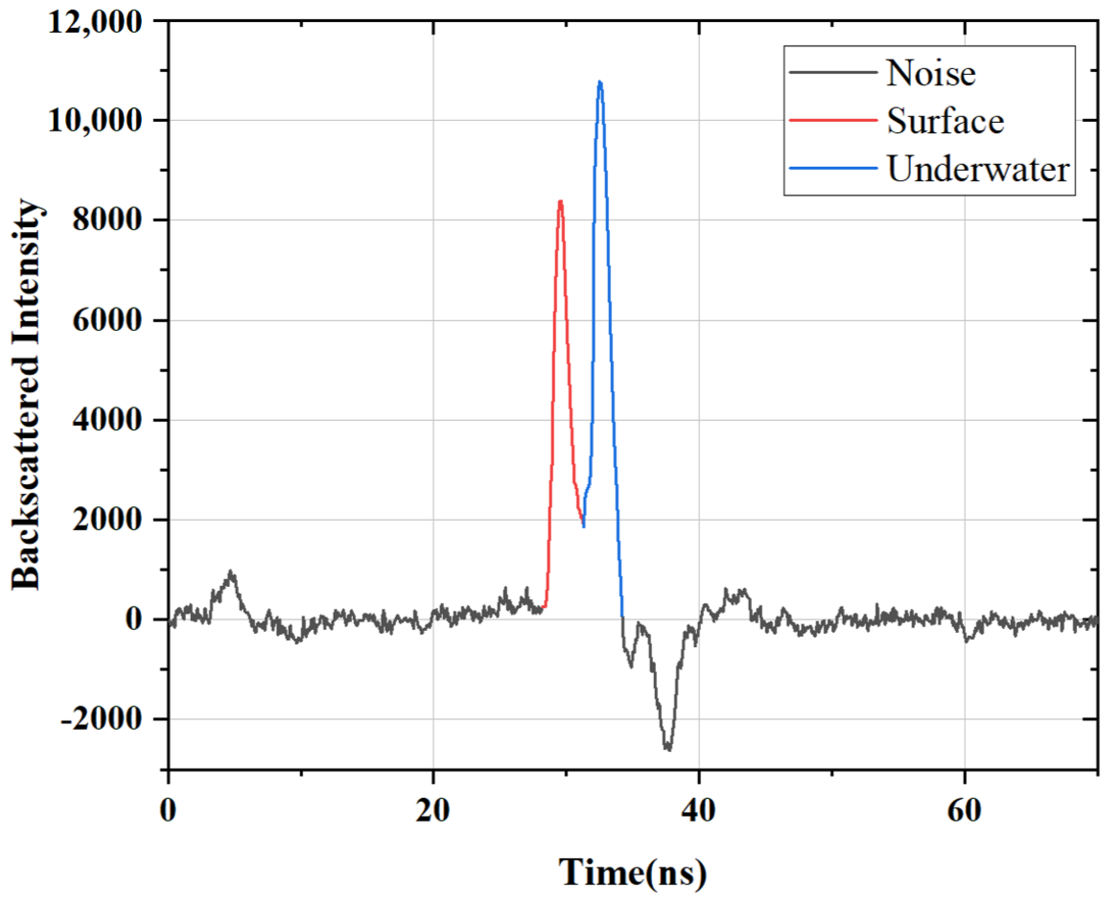
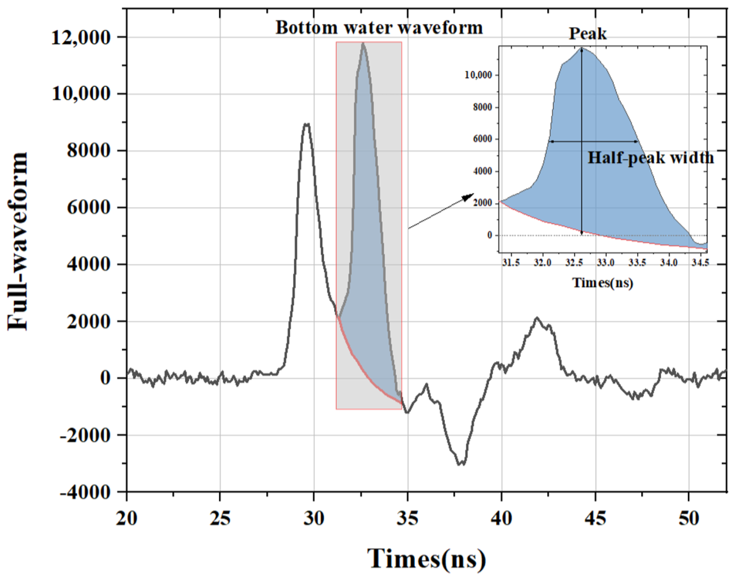
In accordance with the principle of optics, the laser beam is reflected and refracted upon contact with the water surface, subsequently penetrating the water and radiating through it to the seabed. At this point, the beam interacts with various scatterers present in the sediment, resulting in a portion of the laser energy being scattered at different angles and returned to the LiDAR. Accordingly, based on the intensity distribution of the full-waveform data as in Figure 5, the study decomposes the full-waveform data at the water surface and the bottom substrate and analyzes the resulting characteristics.

3.2. Feature Extraction

To establish a stable mapping relationship between the raw optical data and the actual underwater sediment type, it is essential to undertake feature extraction to correctly classify the underwater sediment. In conditions that may be considered ideal (i.e., the LiDAR receiver is composed of an ideal photodiode and the amplifier exhibits wireless bandwidth and linear response), the LiDAR received waveform $\mathrm{s}\left(\mathrm{t}\right)$ is primarily determined by the transmitted waveform $\mathrm{r}\left(\mathrm{t}\right)$ and the surface properties of the illuminated object. The 3D properties of the surface are represented by the transient surface, which is denoted as the surface response $\mathrm{h}\left(\mathrm{t}\right)$ [28]. The received waveform can be expressed as follows:

$$\mathrm{s}\left(\mathrm{t}\right)=\mathrm{h}\left(\mathrm{t}\right)\ast \mathrm{r}\left(\mathrm{t}\right)$$

(1)

where the ∗ denotes convolution. The Fourier transform of the aforementioned equation can be derived as follows:

$$\mathrm{H}\left(f\right)=S\left(f\right)/R\left(f\right)$$

(2)

The typical surface properties extracted from waveforms are found to correspond to the aforementioned waveform attributes, including the range, elevation change, and reflectance of surface properties corresponding to the time, width, and amplitude of the waveform attributes [28]. The amplitude/peak of the waveform is proportional to the backscattered intensity of the irradiated object, which is characterized in the full-waveform data of underwater sediments (as illustrated in Figure 6) using rock samples as an exemplar. The width of the echo/half-peak width is directly correlated with the elevation change and reflectivity of the irradiated object. Furthermore, the peak area serves as an additional means of characterizing the surface properties, such as reflectivity and roughness, of the irradiated object. The distribution pattern of the echo data is typically influenced by the surface roughness of the target (scatterer), exhibiting varying degrees of kurtosis. This feature is quantified by the kurtosis. The scattering characteristics, roughness, and multipath effect of different substrates result in varying echo data distributions and frequency domain performance. This paper employs the main frequency distribution and the sum of energy as the characteristics of the embodiment. Given the significant differences in surface properties among various types of underwater sediments, the time-frequency domain characteristics of LiDAR-received waveforms serve as a crucial basis for assessing the roughness, elevation change, and backward reflection coefficient of the sedimentary surface.

Accordingly, the study extracted waveform features from the echo full-waveform data at the water surface (a) and at the bottom of the water (b), respectively. The extracted features included peak, half-peak width, peak area, kurtosis, and frequency-domain features. The total number of extracted features was 10, as shown in

Table 3. Feature extraction from full-waveform data.

Features	Description	Formula
Peak 1	Characterizes the presence and distribution of scatterers.	$\underset{1\le i\le n}{max}{X}_i$
Half-peak width 1	Characterizes the scale and distribution of the scatterer.	$I_{({\displaystyle \frac{1}{2}}max)r}-I_{({\displaystyle \frac{1}{2}}max)l}$
Peak area 1	Characterizes the hardness and texture of the scatterer.	${\int }_{I_{({\displaystyle \frac{1}{2}}max)l}}^{I_{({\displaystyle \frac{1}{2}}max)r}}X\left(i\right)di$
Kurtosis 1	Characterizes the statistical characteristics of the scatterer.	${\displaystyle \frac{\frac{1}{n}{\displaystyle \sum _{i=1}^n}\left(X_i-\overline{X}{)}^4\right.}{{\left(\frac{1}{n}{\displaystyle \sum _{i=1}^n}\left(X_i-\overline{X}{)}^2\right.\right)}^2}}$
Primary frequency distribution	Characterizes the scattering properties of scatterers and multipath effects.	$F_{\underset{1\le i\le n}{max}{\left|X\left(f\right)\right|}^2}$
Total energy	Characterizes the surface roughness of a scatterer.	${\displaystyle \sum _{i=1}^n}{\left|X\left(f\right)\right|}^2$

¹ Extraction of water surface and bottom features from full-waveform data.

.

Where i is the ith LiDAR full-waveform data, n is the number of sample points, X is the amplitude at the sample point, $\overline{X}$ is the average value of the amplitude at the sample point, and $I_{({\displaystyle \frac{1}{2}}max)r}$ and $I_{({\displaystyle \frac{1}{2}}max)l}$ are the right and left sample points corresponding to half the peak of the LiDAR full-waveform, respectively. X(f) is the Fourier transform of the sequence of LiDAR full-waveform data, and F is the frequency.

3.3. Feature Selection

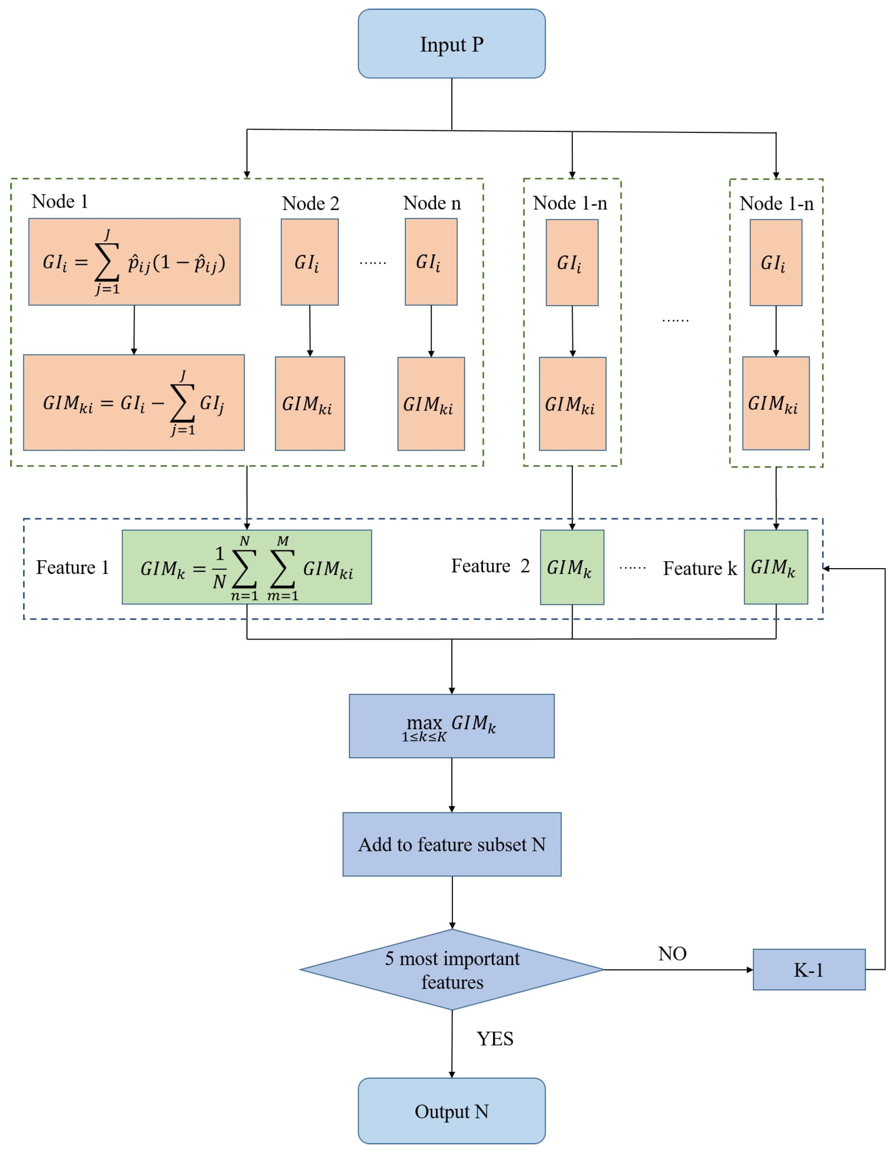
To identify a feature subset from the original feature set that optimizes the retention of spatial information from the original features of underwater sediments, this study employs a combination of Sequential Forward Selection and Random Forests [29] to process the extracted features. This approach facilitates the subsequent classification of underwater sediments, improves the accuracy of the classification, and reduces the time and storage costs [30,31]. Assuming that the original input feature matrix is P, and that the new feature matrix returned after feature selection is N, initially, the new feature matrix N is empty, and the Random Forest algorithm evaluates the importance of the features in the input feature matrix P, and iteratively adds the five most important features to the new feature matrix N. This process is repeated until the new feature matrix N is obtained, which is most beneficial to the classification performance of the Random Forest model and is the optimal feature subset, as shown in Figure 7.

The Random Forest algorithm assesses the significance of features for the classification of underwater sediments by integrating multiple decision trees. The Gini index is a pivotal component in the algorithmic process of integrating sequential forward search with Random Forests. The sequential forward search feature selection method commences with an empty feature set and progressively incorporates features that contribute most to the classification performance. The Gini index, as a metric of feature importance in Random Forests, can efficiently evaluate the contribution of each feature to the classification outcome. In each iteration of feature selection, the Gini index assists in determining the current optimal feature subset. Concurrently, the original feature set obtained from the LiDAR full-waveform data contains a substantial number of high-dimensional features, and the Gini index can evaluate the differentiation ability of each feature to the classification task. This can assist the sequential forward search feature selection algorithm in selecting the most discriminative subset of features in the high-dimensional data, thereby reducing the computational complexity and enhancing the classification efficiency. Prior to the splitting of each node, the Gini index is calculated for each decision tree (3). The reduction in the Gini index is recorded before and after branching the node (4). The importance score is calculated by averaging the Gini indexes across all decision trees (5). A higher score indicates a greater contribution to classification process.

$$G{I}_i=\sum _{j=1}^J{\widehat{p}}_{ij}\left(1-{\widehat{p}}_{ij}\right)$$

(3)

$$GI{M}_{ki}=G{I}_i-\sum _{j=1}^{J}G{I}_j$$

(4)

$$GI{M}_k={\displaystyle \frac{1}{N}}\sum _{n=1}^N\sum _{m=1}^{M}GI{M}_{ki}$$

(5)

where GI refers to the Gini index, while J represents the number of categories in the sample set, which is 4. ${\widehat{p}}_{ij}$ is an estimate of the probability that a sample from node i belongs to j. $GI{M}_{ki}$ refers to the reduction in the Gini index of variable k before and after branching from node i, while $G{I}_j$ denotes the Gini index of each new node after node i splits. Where $GI{M}_k$ represents the Gini importance of variable k, N represents the number of decision trees in the Random Forest, and M represents the number of times variable k appears in the nth tree.

3.4. Random Forest Classification

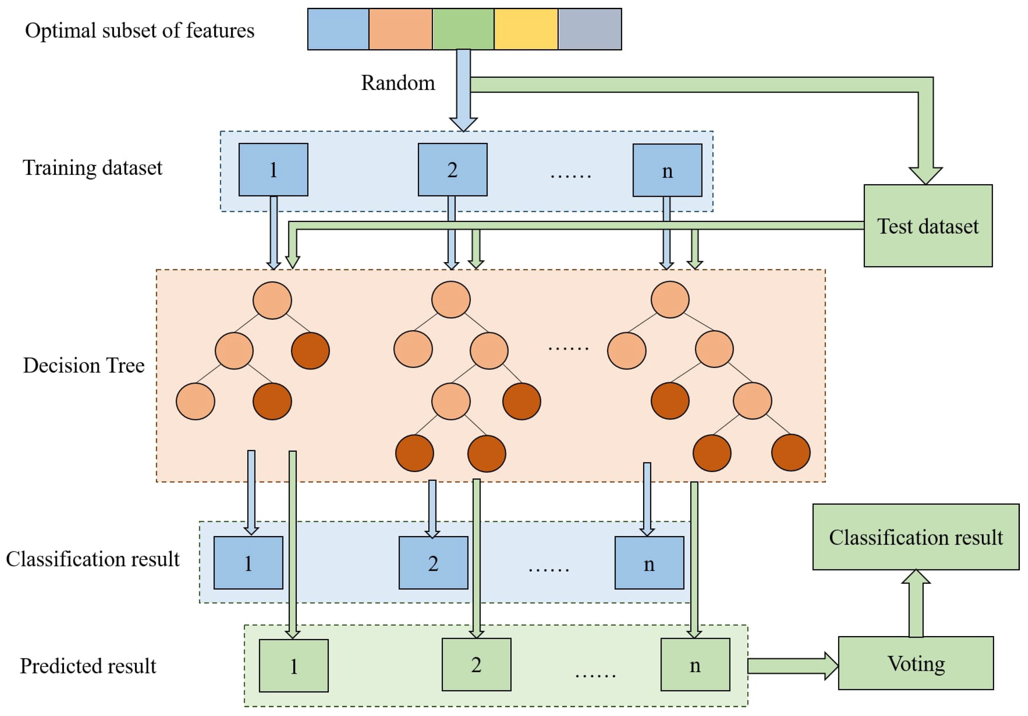
The optimal feature subset is obtained by combining the Sequential Forward Selection feature selection method with the Random Forest classification algorithm. Based on this, a classification model for underwater sediment is constructed using the Random Forest algorithm, which reduces redundant features and improves classification accuracy.

Random Forest [32,33,34] is a machine learning approach that integrates multiple decision trees to perform classification and regression tasks. It is based on the self-sampling approach, and, in this study, it is employed to construct N decision trees by generating N different training datasets. Subsequently, the subsets of the most salient features of the underwater sediment are randomly sampled following the implementation of feature selection with putback. The decision tree is trained by recursively selecting the optimal subset of attributes at each node, thereby obtaining the corresponding classification results for the underwater sediment. In the process of prediction, the decision trees accept unknown samples as input. The prediction is performed based on the selected feature subset and node splitting rules, resulting in a classification for each decision tree. The final classification result is obtained by aggregating the prediction results through a voting procedure, as shown in Figure 8. The Random Forest method is an appropriate approach for the classification of underwater sediments, given its high degree of accuracy and robustness in the context of high-dimensional data. Furthermore, it is particularly effective in addressing the diversity of seabed sediments.

The selection and optimization of hyperparameters in the Random Forest model is imperative, encompassing the number of decision trees, the maximum number of features, the maximum depth, the minimum number of sample splits, and the minimum sample leaf tree. In this study, we methodically set a reasonable range and step size for each hyperparameter, systematically traversed the possible hyperparameter combinations, evaluated the performance using 5-fold cross-validation, calculated the average accuracy, and selected the optimal hyperparameter combination to ensure its robustness.

4. Discussion and Results

In this study, the optimal feature subset was obtained through the application of a feature selection method that integrated Sequential Forward Selection and Random Forest (RF). This subset was then inputted into the Random Forest algorithm for the supervised fast classification of underwater sediment. For the purposes of comparison, the original feature set was combined with the K-Nearest Neighbors (KNN), Support Vector Machine (SVM), and Decision Tree (DT) after Sequential Forward Selection feature selection, and the resulting classification results for each classifier were obtained.

Table 4. Comparison of classification accuracy before and after Sequential Forward Selection feature selection.

Dataset	Feature Selection	KNN	SVM	DT	RF
Overall	/ 1	76.99%	77.39%	91.75%	93.65%
	Sequential Forward Selection	93.20%	93.20%	91.95%	94.10%

¹ No feature selection processing is conducted.

demonstrates that the overall accuracies of the four classification methods was enhanced following the implementation of the Sequential Forward Selection feature selection. This suggests that the algorithm integrating Sequential Forward Selection with classification methods can effectively reduce redundant features and enhance the accuracy of the classification algorithm.

The four classification algorithms, namely K-Nearest Neighbors, Support Vector Machine, Decision Tree, and Random Forest (RF), are employed to classify the original feature set after feature selection. Thereafter, the accuracy of the sample categories, the overall classification accuracy, and the Kappa coefficient are calculated to evaluate each classification model.

A comparative analysis of the experimental results presented in

Table 5. System parameters of the four classifiers after feature selection.

Classifier	Sample Classes	Precision	Overall	Kappa
KNN	mud	99%	93.20%	70.45%
	rock	96%
	sand	55%
	gravel	59%
SVM	mud	99%	93.20%	71.99%
	rock	96%
	sand	59%
	gravel	59%
DT	mud	100%	91.95%	85.77%
	rock	99%
	sand	82%
	gravel	76%
RF	mud	100%	94.10%	91.11%
	rock	100%
	sand	88%
	gravel	85%

, revealed that the combination of Sequential Forward Selection feature selection with each of the four classification methods can efficiently and accurately classify underwater sediments into mud and rock types. Furthermore, the decision tree and Random Forest classification algorithms demonstrated superior efficacy in classifying shallow sand and gravel types of underwater sediments. In particular, the Random Forest algorithm demonstrated significantly higher classification accuracy than the other methods, resulting in an overall classification accuracy of 94.1%, and the Kappa coefficient is 91.11%. These results indicate that the Random Forest algorithm is an effective tool for the high-precision classification of underwater sediment.

Subsequent studies may select representative areas with different types of sediments (e.g., sand, mud, gravel, and rock) in actual shallow sea scenarios to conduct experiments, acquire full-waveform data through LiDAR system detection, and then train, optimize, and improve the model proposed in this study after extracting the features. Furthermore, the test can be gradually expanded to encompass a more comprehensive range of scenarios for comparison and analysis, ultimately encompassing all shallow marine environments. In these environments, the trained model is employed to categorize the sediment of the test area and to obtain information regarding shallow marine sediment.

5. Conclusions

This study proposes a Sequential Forward Selection of LiDAR optical data features in conjunction with Random Forest for underwater sediment classification. The correlation between the full-waveform data and the underwater sediment types is investigated through the simulation of a shallow sea environment and the utilization of a LiDAR system to detect four distinct types of underwater sediment: sand, mud, gravel, and rock. In this study, a feature selection method combining Sequential Forward Selection and classification algorithms was employed to extract waveform and frequency domain features from the full-waveform data and to identify the optimal feature subset for classification.

The results of the experiments demonstrate that this feature extraction method can effectively enhance the accuracy of the classification algorithm. In comparison to other conventional classifiers, including KNN, SVM, and DT, the algorithm that integrates Sequential Forward Selection with Random Forest exhibits superior accuracy and efficiency in underwater sediment classification. This study contributes to the existing body of research on the high-precision classification of shallow sea sediments using optical data features derived from LiDAR bathymetry technology. The findings provide a valuable foundation for further research into the marine environment and geological resources. The findings of this research are significant for several fields, including marine geological research, resource development, environmental monitoring and protection, and construction engineering.