3D Dubins Curve-Based Path Planning for UUV in Unknown Environments Using an Improved RRT* Algorithm

Abstract

The autonomous navigation of an Unmanned Underwater Vehicle (UUV) in unknown 3D underwater environments remains a challenging task due to the presence of complex terrain, uncertain obstacles, and strict kinematic constraints. This paper proposes a novel smooth path planning framework that integrates improved Rapidly-exploring Random Tree* (RRT*) with 3D Dubins curves to efficiently generate feasible and collision-free trajectories for nonholonomic UUVs. A fast curve-length estimation approach based on a backpropagation neural network is introduced to reduce computational burden during path evaluation. Furthermore, the improved RRT* algorithm incorporates pseudorandom sampling, terminal node backtracking, and goal-biased exploration strategies to enhance convergence and path quality. Extensive simulation results in unknown underwater scenarios with static and moving obstacles demonstrate that the proposed method significantly outperforms state-of-the-art planning algorithms in terms of smoothness, path length, and computational efficiency.

1. Introduction

The maritime environment presents significant challenges for autonomous systems, including uncertain weather, limited visibility, and high operational risk [1,2]. In recent years, Unmanned Underwater Vehicle (UUV) technology has seen rapid development in recent years, offering promising capabilities in marine exploration, environmental monitoring, infrastructure inspection, and defense applications [3,4,5,6]. Real-time path planning for an UUV is challenging due to the complexity of unknown underwater environments and the vehicle’s nonholonomic constraints. To enable fully autonomous operations in such conditions, a robust path planning system must generate feasible and smooth trajectories while ensuring collision avoidance in dynamic and cluttered surroundings.

Persistent efforts have been made to address the prescribed disadvantages [7,8,9]. In [8], a collision-free navigation method for dynamic environments was proposed. This method constructs a probabilistic graph model of the workspace and combines the A* search algorithm with the potential field method to generate feasible maneuvering paths. In [9], a two-stage path planning approach was introduced to guide a robot operating in a partially known environment. The approach first builds a visibility graph of the static environment and uses the Dijkstra algorithm to determine a global path. During the path-following phase, a dual-strategy fuzzy controller is employed to continuously generate local collision-free maneuvering paths. In [10], an efficient convex decomposition method was proposed, which divides the free space into convex polyhedral regions and utilizes the Jump Point Search algorithm to plan safe paths. However, these methods rely on search algorithms to determine resulting paths in structured and static environments, making them inefficient when applied to high-dimensional settings.

In recent years, sampling-based path planning methods have gained increasing attention, particularly incremental sampling techniques such as the Rapidly-exploring Random Tree (RRT) and its improved variant, RRT* [11]. These algorithms incrementally construct collision-free trajectories by sampling the configuration space rather than searching over a grid or structured map, allowing them to perform well in unstructured and high-dimensional environments. Their generated paths typically converge probabilistically to an optimal solution. In [12], an asymptotically optimal motion planning method was proposed for robots with linear dynamics, using the RRT* algorithm for global planning and generating sample trajectories between state pairs via an optimal controller. In [13], the RRT* algorithm was enhanced by narrowing the sampled state set, improving performance in finding near-optimal solutions. These approaches primarily focus on static environments. To address dynamic obstacles, Ref. [14] proposed a hybrid method combining an improved Dynamic Window Approach (DWA) with RRT* to plan both global paths and local trajectories for UUVs in dynamic settings. In [15], RRT* was integrated with Bézier curves to achieve path planning in environments with unknown obstacles.

Despite these advances, several challenges remain in the application of incremental sampling-based path planners. First, the generated maneuvers are often vulnerable to unexpected environmental changes, which can lead to wasted computational effort and increased planning cost during replanning. Second, generating a sufficient number of reachable sample nodes is critical for adequately exploring the environment and producing collision-free maneuvers. However, this process can be computationally inefficient and time-consuming due to kinematic constraints and the presence of environmental obstacles [16,17].

To address the aforementioned limitations, this paper proposes a smooth path planning method for UUVs in unknown 3D environments, which integrates an improved RRT* algorithm with 3D Dubins curves. The proposed method operates under a reactive planning and replanning framework to accommodate environmental uncertainty and the absence of prior information. During replanning, collision-free segments of previously generated paths are reused as structural foundations, while smooth maneuver trajectories are constructed after a coarse path is generated using the enhanced RRT*. To improve planning efficiency, the enhanced RRT* algorithm incorporates pseudorandom sampling, terminal node backtracking-based extension, and goal-biased exploration as key procedures, while 3D Dubins curves are employed to guide the path generation process. Finally, a fast and efficient path reshaping process ensures the resulting trajectory is both smooth and collision-free. The main contributions of this paper are summarized as follows:

• The geometric characteristics of 3D Dubins curves are analyzed, and a Backpropagation Neural Network (BPNN) is designed to enable fast length estimation of these curves.
• A pseudorandom sampling strategy is developed to enhance obstacle avoidance performance during node generation in cluttered underwater environments.
• A novel terminal node backtracking mechanism is introduced to maintain the spatio-temporal feasibility of the tree expansion process in dynamic scenarios.

The remainder of this paper is organized as follows: Section 2 presents the problem formulation and mathematical preliminaries. Section 3 describes the proposed path planning method in detail. Simulation results and comparative analysis are shown in Section 4. Finally, Section 5 concludes the paper.

2. Mathematical Formulation

2.1. Problem Statement

The operational environment is denoted by $\mathcal{X}$, which consists of the obstacle region ${\mathcal{X}}_o$ and the collision-free region ${\mathcal{X}}_f$. It should be pointed out that there may be both static obstacles and moving obstacles in ${\mathcal{X}}_o$. The obstacle region ${\mathcal{X}}_o$ may include both static and dynamic obstacles. To facilitate computational tractability in path planning, all obstacles are modeled as spheres ${\mathcal{X}}_o$, following the approach in  [18,19]. The i-th spherical obstacle is denoted by ${\Omega }_i$, with its occupied region at time t defined as

$${\Omega }_i\left(t\right)=\left\{\mathbf{p}\left(t\right)|\parallel \mathbf{p}\left(t\right)-{\mathbf{o}}_i\left(t\right)\parallel \le r_i+\delta \right\}.$$

(1)

where ${\mathbf{o}}_i$ denotes the center of the obstacle, $r_i$ is its radius, and $\delta$ represents a safety margin reserved for path planning. The complete obstacle region ${\mathcal{X}}_o$ can be defined as

$${\mathcal{X}}_o=\bigcup _{i=1}^{N_{obs}}{\Omega }_i$$

(2)

where $N_{obs}$ denotes the total number of the spherical obstacles. If obstacle i is a moving obstacle, ${\mathbf{v}}_{{obs}_i}$ represents its velocity.

To describe the motion of the UUV, let $\mathbf{p}$ denote its current position in three-dimensional space. The velocity and configuration associated with position $\mathbf{p}$ are represented by $\mathcal{V}\left(\mathbf{p}\right)$ and $\mathcal{C}\left(\mathbf{p}\right)$, respectively, where $\mathcal{V}\left(\mathbf{p}\right)$ returns the velocity vector, and $\mathcal{C}\left(\mathbf{p}\right)$ describes the UUV’s orientation and heading at that position. In this work, the UUV is modeled as a three-dimensional nonholonomic system subject to constant forward speed and no lateral slip, an assumption consistent with Dubins motion primitives in underwater environments. Accordingly, the heading direction of the UUV is determined by its velocity vector $\mathcal{V}\left(\mathbf{p}\right)$. The kinematic constraint of the UUV is characterized by a minimum turning radius, denoted as $r_{min}$, which defines the tightest possible curvature of its trajectory while maintaining feasible underwater motion dynamics.

To formulate the smooth path planning problem in an unknown underwater environment, it is assumed that the UUV can only perceive obstacle motion information within a limited sensing radius, denoted by $r_{\mathrm{scan}}$. Under this constraint, the objective of path planning is to compute a sufficiently smooth and collision-free path $\mathbf{L}$ that leads the UUV from its current configuration to the target configuration $\mathcal{C}\left({\mathbf{p}}_{\mathrm{goal}}\right)$. This problem can be mathematically expressed as the minimization of the path length subject to obstacle avoidance constraints

$$\underset{\mathbf{L}\cancel{\cap }{\mathcal{X}}_o}{argmin}\parallel \mathbf{L}\parallel .$$

(3)

2.2. 3D Dubins Curve Determination

Smooth trajectory generation is critical for UUV path planning, especially under nonholonomic constraints. Commonly used smooth curves include Bézier and B-spline curves, which offer high-order continuity and visual smoothness. However, these curves do not inherently satisfy curvature or heading constraints, and enforcing such constraints often requires additional optimization or post-processing.

In contrast, Dubins curves are specifically constructed to model motion with constant forward velocity and a minimum turning radius, making them a natural fit for nonholonomic vehicles such as UUVs. Therefore, this work adopts 3D Dubins curves as the motion primitive to ensure dynamically feasible and computationally efficient trajectory planning.

Dubins curves are composed of a combination of circular (C) and straight-line (S) segments. In two-dimensional space, the Dubins curve has been proven to provide the shortest feasible path between two specified configurations under a minimum turning radius constraint, making it the optimal solution for smooth path planning in planar environments [20,21,22,23]. However, in three-dimensional or higher-dimensional spaces, the construction of Dubins curves becomes more complex due to the increased number of feasible path configurations and geometric constraints. To address these challenges, this study introduces an efficient numerical technique for constructing 3D Dubins curves by leveraging their geometric properties.

For notational convenience, two auxiliary functions are defined. The normalization function $\mathbf{n}\left(\mathbf{v}\right)$ returns the unit vector in the direction of vector $\mathbf{v}$, and the sign function $Sgn\left(x\right)$ returns the sign of scalar x. Given the practical significance of 3D Dubins curves in underwater path planning, the geometrical analysis in this paper focuses on the CSC (curve–straight–curve) configuration, which is commonly encountered in optimal Dubins paths [24]. Other configuration types can be derived using a similar approach and are not elaborated here for brevity.

As illustrated in Figure 1, a CSC Dubins path connects two spatial configurations, $\mathcal{C}\left({\mathbf{p}}_1\right)$ and $\mathcal{C}\left({\mathbf{p}}_2\right)$, with its straight segment intersecting the initial and terminal circular arcs at points ${\mathbf{p}}_{C_1}$ and ${\mathbf{p}}_{C_2}$, respectively. Two auxiliary lines, $L_1$ and $L_2$, are constructed to pass through ${\mathbf{p}}_1$ and ${\mathbf{p}}_2$, respectively, and they are aligned with the initial and terminal velocity directions ${\mathcal{C}}_1$ and ${\mathcal{C}}_2$. The direction vector of the straight segment (S) is then given by ${\mathbf{v}}_s=\mathbf{n}\left({\mathbf{p}}_{C_2}-{\mathbf{p}}_{C_1}\right)$. Let L denote the line extending the straight segment. This line intersects with $L_1$ and $L_2$ at points ${\mathbf{p}}_{L_1}$ and ${\mathbf{p}}_{L_2}$, respectively, where ${\mathbf{p}}_{L_1}\ne {\mathbf{p}}_{L_2}$. The analytical expressions for these intersection points can be derived as

$$\left\{\begin{array}{c}\hfill {\mathbf{p}}_{L_1}={\mathbf{p}}_1+k_1\mathcal{V}\left({\mathbf{p}}_1\right)\\ \hfill {\mathbf{p}}_{L_2}={\mathbf{p}}_2+k_2\mathcal{V}\left({\mathbf{p}}_2\right)\end{array}\right.$$

(4)

where $k_1$ and $k_2$ are two nonzero constants.

Let the centers of the initial and terminal circular segments $C_1$ and $C_2$ be denoted by ${\mathbf{o}}_1$ and ${\mathbf{o}}_2$, respectively. Due to the geometric property of Dubins curves, there are always ${\mathbf{o}}_1{\mathbf{p}}_1\perp {\mathbf{p}}_{L_1}{\mathbf{p}}_{C_1}$ and ${\mathbf{o}}_2{\mathbf{p}}_2\perp {\mathbf{p}}_{L_2}{\mathbf{p}}_{C_2}$. It derives that ${\mathbf{p}}_{C_1}={\mathbf{p}}_{L_1}+k_1{\mathbf{v}}_s$ and ${\mathbf{p}}_{C_2}={\mathbf{p}}_{L_2}+k_2{\mathbf{v}}_s$. Thus, the direction vector ${\mathbf{v}}_s$ of the straight segment can be written as

$${\mathbf{v}}_s=\mathbf{n}\left(\delta \mathbf{p}+k_2\left(\mathcal{V}\left({\mathbf{p}}_2\right)+{\mathbf{v}}_s\right)-k_1\left(\mathcal{V}\left({\mathbf{p}}_1\right)+{\mathbf{v}}_s\right)\right)$$

(5)

where $\delta \mathbf{p}={\mathbf{p}}_2-{\mathbf{p}}_1$ denotes the displacement vector between the initial and terminal positions. Equation (5) can be further reformulated as

$${\mathbf{v}}_s=\pm \left(\delta \mathbf{p}+k_2\mathcal{V}\left({\mathbf{p}}_2\right)-k_1\mathcal{V}\left({\mathbf{p}}_1\right)\right)/\mathrm{m}\left(k_1,k_2\right)$$

(6)

where $\mathrm{m}\left(k_1,k_2\right)$ represents the normalization factor, defined as

$$\mathrm{m}\left(k_1,k_2\right)=\sqrt{A+k_1^2+k_2^2+2k_2{B}_2-2k_1{B}_1-2k_1{k}_2{B}_{12}}$$

(7)

with the scalar quantities given by $A={\left|\delta \mathbf{p}\right|}^2$, $B_2=\mathcal{V}\left({\mathbf{p}}_2\right)·\delta \mathbf{p}$, $B_1=\mathcal{V}\left({\mathbf{p}}_1\right)·\delta \mathbf{p}$ and $B_{12}=\mathcal{V}\left({\mathbf{p}}_1\right)·\mathcal{V}\left({\mathbf{p}}_2\right)$. Furthermore, Equation (6) implies that the inequality

$${\mathbf{v}}_s=\mathbf{s}\left(k_2-k_1\pm \mathrm{m}\left(k_1,k_2\right)\right){\mathbf{v}}_s$$

(8)

Obviously, Equation (8) demands that $k_2-k_1\pm \mathrm{m}\left(k_1,k_2\right)>0$ holds for CSC Dubins curves. Hence, if $q(k_1,k_2)$ denotes $A+2k_2{B}_2-2k_1{B}_1+2k_1{k}_2\left(1-B_{12}\right)$, the establishment conditions of CSC curves are as presented in

Table 1. Establishment conditions of CSC curves.

Case	${\mathit{v}}_{\mathit{s}}$	${\mathit{k}}_1\&{\mathit{k}}_2$	Condition
Case 1	${\displaystyle \frac{\delta \mathbf{p}+k_2\mathcal{V}\left({\mathbf{p}}_2\right)-k_1\mathcal{V}\left({\mathbf{p}}_1\right)}{\mathrm{m}\left(k_1,k_2\right)}}$	$k_2\ge k_1$	none
Case 2		$k_2<k_1$	$q(k_1,k_2)>0$
Case 3	$-{\displaystyle \frac{\delta \mathbf{p}+k_2{\overrightarrow{V}}_2-k_1{\overrightarrow{V}}_1}{\mathrm{m}\left(k_1,k_2\right)}}$	$k_2>k_1$	$q(k_1,k_2)<0$

.

Two auxiliary unit vectors, ${\mathbf{n}}_1$ and ${\mathbf{n}}_2$, are introduced to represent the normal directions from the initial and terminal configurations to their respective circular arc centers. These vectors are defined as

$$\left\{\begin{array}{c}\hfill {\mathbf{n}}_1=\mathbf{s}\left(k_1\right)\mathbf{n}\left(\mathcal{V}\left({\mathbf{p}}_1\right)\times {\mathbf{v}}_s\times \mathcal{V}\left({\mathbf{p}}_1\right)\right),\\ \hfill {\mathbf{n}}_2=\mathbf{s}\left(k_2\right)\mathbf{n}\left(\mathcal{V}\left({\mathbf{p}}_2\right)\times {\mathbf{v}}_s\times \mathcal{V}\left({\mathbf{p}}_2\right)\right).\end{array}\right.$$

(9)

where $\mathbf{s}(·)$ denotes the sign function that ensures correct orientation, and $\mathbf{n}(·)$ denotes the normalization operator.

Accordingly, the circular centers of $C_1$ and $C_2$ can be expressed as ${\mathbf{o}}_1={\mathbf{p}}_1+r_1{\mathbf{n}}_1$ and ${\mathbf{o}}_2={\mathbf{p}}_2+r_2{\mathbf{n}}_2$. Considering the spatial relations of ${\mathbf{o}}_1$ and ${\mathbf{o}}_2$ with ${\mathbf{p}}_{C_1}$ and ${\mathbf{p}}_{C_2}$, there are $|k_1(\mathcal{V}\left({\mathbf{p}}_1\right)+{\mathbf{v}}_s)-r_1{\mathbf{n}}_1|=r_1$ and $|k_2(\mathcal{V}\left({\mathbf{p}}_2\right)+{\mathbf{v}}_s)-r_2{\mathbf{n}}_2|=r_2$.

Furthermore, since the CSC curve is smooth at ${\mathbf{p}}_{C_1}$ and ${\mathbf{p}}_{C_2}$, it derives that ${\mathbf{v}}_s=\mathbf{s}\left(k_1\right)\mathbf{n}\left(\mathcal{V}\left({\mathbf{p}}_1\right)\times {\mathbf{v}}_s\times {\mathbf{o}}_1{\mathbf{p}}_{C_1}\right)$ and ${\mathbf{v}}_s=\mathbf{s}\left(k_2\right)\mathbf{n}\left(\mathcal{V}\left({\mathbf{p}}_2\right)\times {\mathbf{v}}_s\times {\mathbf{o}}_2{\mathbf{p}}_{C_2}\right)$. Given that ${\mathbf{v}}_s$ is orthogonal to $\overrightarrow{{\mathbf{o}}_1{\mathbf{p}}_{C_1}}$ and $\overrightarrow{{\mathbf{o}}_2{\mathbf{p}}_{C_2}}$, the following conditions must be satisfied: $k_1{\mathbf{v}}_s·\mathcal{V}\left({\mathbf{p}}_1\right)+k_1-r_1{\mathbf{v}}_s·{\mathbf{n}}_1=0$ and $k_2{\mathbf{v}}_s·\mathcal{V}\left({\mathbf{p}}_2\right)+k_2-r_2{\mathbf{V}}_s·{\mathbf{n}}_2=0$.

If ${\mathbf{v}}_s\ne -\mathcal{V}\left({\mathbf{p}}_1\right)$ and ${\mathbf{v}}_s\ne -\mathcal{V}\left({\mathbf{p}}_2\right)$, that is to say $k_1\ne +\infty$ and $k_2\ne -\infty$, there are

$$\left\{\begin{array}{c}\hfill \left(r_1^2-k_1^2\right)/\left(k_1^2+r_1^2\right)=\pm \left(B_1+k_2{B}_{12}-k_1\right)/\mathrm{m}\left(k_1,k_2\right)\\ \hfill \left(r_2^2-k_2^2\right)/\left(k_2^2+r_2^2\right)=\pm \left(B_2+k_2-k_1{B}_{12}\right)/\mathrm{m}\left(k_1,k_2\right)\end{array}\right.$$

(10)

where $\mathrm{m}(k_1,k_2)$ is defined in the previous subsection, and $B_1$, $B_2$, and $B12$ are the projection coefficients introduced earlier. By solving the nonlinear system in (10) under the existence conditions summarized in Table 1, feasible pairs of $(k_1,k_2)$ can be determined. Each solution corresponds to a candidate CSC-type 3D Dubins curve. The total length of each candidate curve is obtained by summing the lengths of its component segments. The shortest among them defines the optimal Dubins path. For clarity in notation, we denote the 3D Dubins curve connecting $\mathcal{C}\left({\mathbf{p}}_i\right)$ and $\mathcal{C}\left({\mathbf{p}}_j\right)$ as ${\mathcal{T}}_{ij}$, and its total length as ${\mathcal{T}}_{ij}$.

Remark 1. 

The 3D Dubins curve between ${\mathcal{C}}_1$ and ${\mathcal{C}}_2$ with given $r_1$ and $r_2$ is decided by $k_1$ and $k_2$, specifically, by A, $B_2$, $B_1$, and $B_{12}$.

To concisely characterize the geometry of a 3D Dubins curve, we define its geometric descriptor vector as ${\Lambda }_{\mathcal{T}}=[A,B_1,B_2,B_{12},r_1,r_2]$.

2.3. Fast 3D Dubins Curve Length Estimation

To reduce the computational overhead of sample-based path planning, this paper proposes a fast 3D Dubins curve length estimation method based on a Backpropagation Neural Network (BPNN). As stated in Remark 1, a 3D Dubins curve is uniquely determined by its geometric character vector ${\Lambda }_{\mathcal{T}}$. Leveraging this property, the BPNN takes ${\Lambda }_{\mathcal{T}}$ as its input and outputs an estimated curve length, enabling efficient evaluation without solving the full geometric model. The structure of the proposed BPNN is illustrated in Figure 2. It consists of 1 input layer with 6 elements, 2 hidden layers with 30 and 22 tansig neurons, and 1 output layer with a purelin neuron.

To train the proposed BPNN, a dataset comprising 10,000 3D Dubins curves was generated. Each curve connects two randomly sampled configurations, with the Euclidean distance between positions satisfying $\left|\delta \mathbf{p}\right|\in [2(r_1+r_2),4(r_1+r_2)]$ and turning radii $r_i\in \{1,2,3\}$. The network was trained using $90\%$ of the dataset, while the remaining $10\%$ was used for testing.

To quantitatively evaluate the generalization capability of the trained model, we generated four independent test groups, each consisting of 1000 new 3D Dubins curves. The BPNN-estimated lengths were compared with the numerically computed ground truth values. As summarized in

Table 2. Computation time and error comparison.

Group	Numerical Method	BPNN Method	Avg. Rel. Error
1	39.6973 s	0.2033 s	4.77%
2	38.6567 s	0.1941 s	4.79%
3	38.0622 s	0.1948 s	4.47%
4	39.3130 s	0.1969 s	4.02%

, the proposed method achieves an average relative error under $5\%$ in all test groups, and it demonstrates a computational speedup of nearly $200\times$ compared to traditional numerical methods.

To further illustrate estimation accuracy, Figure 3 shows a detailed curve-wise comparison of computed and estimated lengths for Group 2. The estimated curve follows the ground truth closely across the sampled experiments, confirming the method’s reliability.

Additionally, Figure 4 presents full comparison plots across all four test groups. Each subplot displays the estimated and computed Dubins lengths over 1000 samples. The BPNN consistently captures the global distribution and local variation of Dubins curve lengths, validating its generalization ability.

Across these four experiments, the average relative errors were 4.77%, 4.79%, 4.47%, and 4.02%, respectively. Moreover, the maximum absolute errors observed were 13.15%, 11.79%, 13.11%, and 6.61%—all within acceptable bounds. These results demonstrate that the proposed method offers an excellent trade-off between estimation speed and accuracy. The estimated length of the Dubins path between $\mathcal{C}\left({\mathbf{p}}_i\right)$ and $\mathcal{C}\left({\mathbf{p}}_j\right)$ is denoted as ${\widehat{\mathcal{T}}}_{i,j}$ throughout this paper, and it is used in the subsequent planning procedures.

3. Efficient Smooth Path Planning

3.1. Overview

The RRT* algorithm is an incremental, sampling-based path planning method, as presented in Algorithm 1, and it guarantees asymptotic global optimality. Inspired by RRT*-based algorithms, this work addresses the problem of smooth path planning, particularly in unknown environments. To ensure the path planning and replanning performance in unknown environments, it takes three aspects of improvements as follows.

From the perspective of implementation, the proposed smooth path planning approach is designed to be responsive to changes in the feasibility of the current path, as illustrated in Figure 5. To improve the efficiency of both path planning and replanning, a hybrid mechanism combining path reuse, rough path planning, and path reshaping is employed. During the path reuse phase, the feasible segment of the previously planned path is retained and utilized to accelerate the replanning process. Subsequently, the precise computation of Dubins curves is deferred, and an enhanced RRT* algorithm is adopted to rapidly generate a rough path, thereby significantly reducing computational overhead. Finally, smooth and kinematically feasible maneuvers are produced by reshaping the rough trajectory based on the motion constraints of the UUV.  

Algorithm 1: RRT* Algorithm

1: $V\leftarrow \mathbf{p}\left(0\right)$, $\left\{\mathcal{E}\right\}\leftarrow \varnothing$ 2: for  $i=1,2,...,n$  do 3:    randomly sample in ${\mathcal{X}}_f$ and obtain ${\mathbf{p}}_{rand}$ 4:    ${\mathbf{p}}_{nst}\leftarrow \underset{\mathbf{p}\in \mathcal{G}}{argmin}\parallel \mathbf{p}-{\mathbf{p}}_{rand}\parallel$ 5:    steer from ${\mathbf{p}}_{nst}$ towards ${\mathbf{p}}_{rand}$ and obtain ${\mathbf{p}}_{new}$ 6:    if $\mathcal{E}\left({\mathbf{p}}_{nst},{\mathbf{p}}_{new}\right)$ is collision-free then 7:      $\left\{{\mathbf{p}}_{near}\right\}\leftarrow \mathbf{p}\in \mathcal{G}$ and $\parallel \mathbf{p}-{\mathbf{p}}_{new}\parallel$ 8:      $\mathcal{G}\leftarrow {\mathbf{p}}_{new}$ and $\left\{\mathcal{E}\right\}\leftarrow \mathcal{E}\left({\mathbf{p}}_{nst},{\mathbf{p}}_{new}\right)$ 9:      for ${\mathbf{p}}_{near}\in \left\{{\mathbf{p}}_{near}\right\}$ and $\mathcal{E}\left({\mathbf{p}}_{near},{\mathbf{p}}_{new}\right)$ is collision-free do 10:         if $t\left({\mathbf{p}}_{near}\right)+\parallel \mathcal{E}\left({\mathbf{p}}_{near},{\mathbf{p}}_{new}\right)\parallel <t\left({\mathbf{p}}_{new}\right)$ then 11:           set ${\mathbf{p}}_{near}$ as the parent node of ${\mathbf{p}}_{new}$ 12:           delete $\mathcal{E}\left({\mathbf{p}}_{nst},{\mathbf{p}}_{new}\right)$ and $\left\{\mathcal{E}\right\}\leftarrow \mathcal{E}\left({\mathbf{p}}_{near},{\mathbf{p}}_{new}\right)$ 13:         end if 14:      end for 15:      for ${\mathbf{p}}_{near}\in \left\{{\mathbf{p}}_{near}\right\}$ and $\mathcal{E}\left({\mathbf{p}}_{new},{\mathbf{p}}_{near}\right)$ is collision-free do 16:         if $t\left({\mathbf{p}}_{new}\right)+\parallel \mathcal{E}\left({\mathbf{p}}_{new},{\mathbf{p}}_{near}\right)\parallel <t\left({\mathbf{p}}_{near}\right)$ then 17:           $\mathcal{G}\leftarrow {\mathbf{p}}_{new}$ and $\left\{\mathcal{E}\right\}\leftarrow \mathcal{E}\left({\mathbf{p}}_{nst},{\mathbf{p}}_{new}\right)$ 18:         end if 19:      end for 20:    end if 21: end for

The improved RRT* algorithm still utilizes a random tree structure as the foundation for path generation. However, it further incorporates the concept outlined in Remark 2.

Remark 2. 

Each terminal node maintains a unique path from the root node.

Motivated by this property, terminal nodes are used to represent the growth state of the tree in the improved RRT* algorithm. These nodes are classified based on their roles in the planning process and stored in the following three sets: $V_{new}$, $V_{open}$, and $V_{close}$. Specifically, $V_{new}$ contains nodes whose expansion is impeded by obstacles, $V_{open}$ includes nodes that are eligible for further extension, and $V_{close}$ holds nodes that have feasible paths to the goal configuration. Accordingly, the improved RRT* algorithm guides the sampling, expansion, and exploration processes using $V_{open}$ and $V_{new}$, while maintaining feasible path candidates in $V_{close}$. From an algorithmic perspective, the processes of sampling, expansion, and exploration are also enhanced. To improve the efficiency of generating feasible trajectories in cluttered or partially known underwater environments, collision-checking information is embedded into the pseudorandom sampling strategy. Additionally, a terminal-node backtracking mechanism is introduced to preserve tree connectivity in the presence of moving or newly discovered obstacles during expansion. The exploration process is further accelerated through a goal-biased strategy, activated under specific maturity conditions.

For clarity and ease of reference, the fundamental variables and their corresponding definitions are summarized in

Table 3. Nomenclature of variables in the improved RRT* algorithm.

Variable	Definition
$t\left(\mathbf{p}\right)$	Return the path length from root to $\mathcal{C}\left(\mathbf{p}\right)$
${\mathcal{D}}_{i,j}$	Straight line segment that connects ${\mathbf{p}}_i$ and ${\mathbf{p}}_j$
${\mathcal{R}}_{i,...j,k}$	Unsmoothed path from root to ${\mathbf{p}}_k$ via ${\mathbf{p}}_i,...,{\mathbf{p}}_j$
$\mathcal{Q}\left(\mathbf{p}\right)$	Return the collision detection result stored at $\mathcal{C}\left(\mathbf{p}\right)$
$\mathcal{F}\left(\mathbf{p}\right)$	Return the parent node of $\mathcal{C}\left(\mathbf{p}\right)$
${\mathcal{L}}_{i,...,j,k}$	Smooth path from root to $\mathcal{C}\left({\mathbf{p}}_k\right)$ via $\mathcal{C}\left({\mathbf{p}}_i\right),...,\mathcal{C}\left({\mathbf{p}}_j\right)$
$\mathcal{G}$	Random tree for path planning

.

3.2. Collision Detection

Collision detection is a fundamental procedure in both path planning and replanning. It verifies the feasibility of candidate maneuvers and determines whether path re-computation is necessary. To enhance the efficiency of the planning process, this paper introduces the concept of maximal collision, which provides a quantitative assessment of collision detection results. For a spherical obstacle ${\Omega }_i$, a collision with the UUV occurs if the following condition is satisfied

$$\underset{\mathbf{p}\left(t\right)\in \mathbf{L}}{argmin}\parallel \mathbf{p}\left(t\right)-{\mathbf{o}}_i\left(t\right)\parallel <r_i$$

(11)

Similarly, in an environment containing multiple obstacles, the maneuver $\mathbf{L}$ is considered infeasible if condition (11) is satisfied for any detected obstacle. This leads to the introduction of the maximal collision concept, which identifies the obstacle that first causes a collision as the maximal collision obstacle, denoted by $i_{max}$. Furthermore, the maximal collision time is defined as the moment when the distance between the UUV and the center of the maximal collision obstacle reaches its minimum. Let $t_{max}$ denote the maximal collision time. Then,

$$t_{max}=\underset{i\le N_{obs}}{argmin}\parallel \mathbf{p}\left(t\right)-{\mathbf{o}}_{i_{max}}\left(t\right)\parallel$$

(12)

3.3. Path Reuse

Once present path is evaluated to be infeasible, its feasible part can be obtained and denoted by ${\mathbf{L}}_f$, which starts from the present configuration of the UUV and ends at the last reachable configuration before the maximal collision occurs. ${\mathbf{L}}_f$ is reused as the initial part of the random tree and the other part of $\mathbf{L}$ is discarded.

To reuse ${\mathbf{L}}_f$ in the improved RRT* algorithm, the nodes of ${\mathbf{L}}_f$ are recorded in $V_{new}$ and the collision detection result of ${\mathbf{L}}_f$ are assigned to these nodes as well. Thus, new branches will grow from multiple nodes to avoid the obstructions. The smooth connections between the reachable nodes are saved as well, and the present configuration of the UUV is set as the root node of $\mathcal{G}$ which can be written as $\mathcal{C}\left({\mathbf{p}}_0\right)$.

3.4. Improved RRT* Algorithm

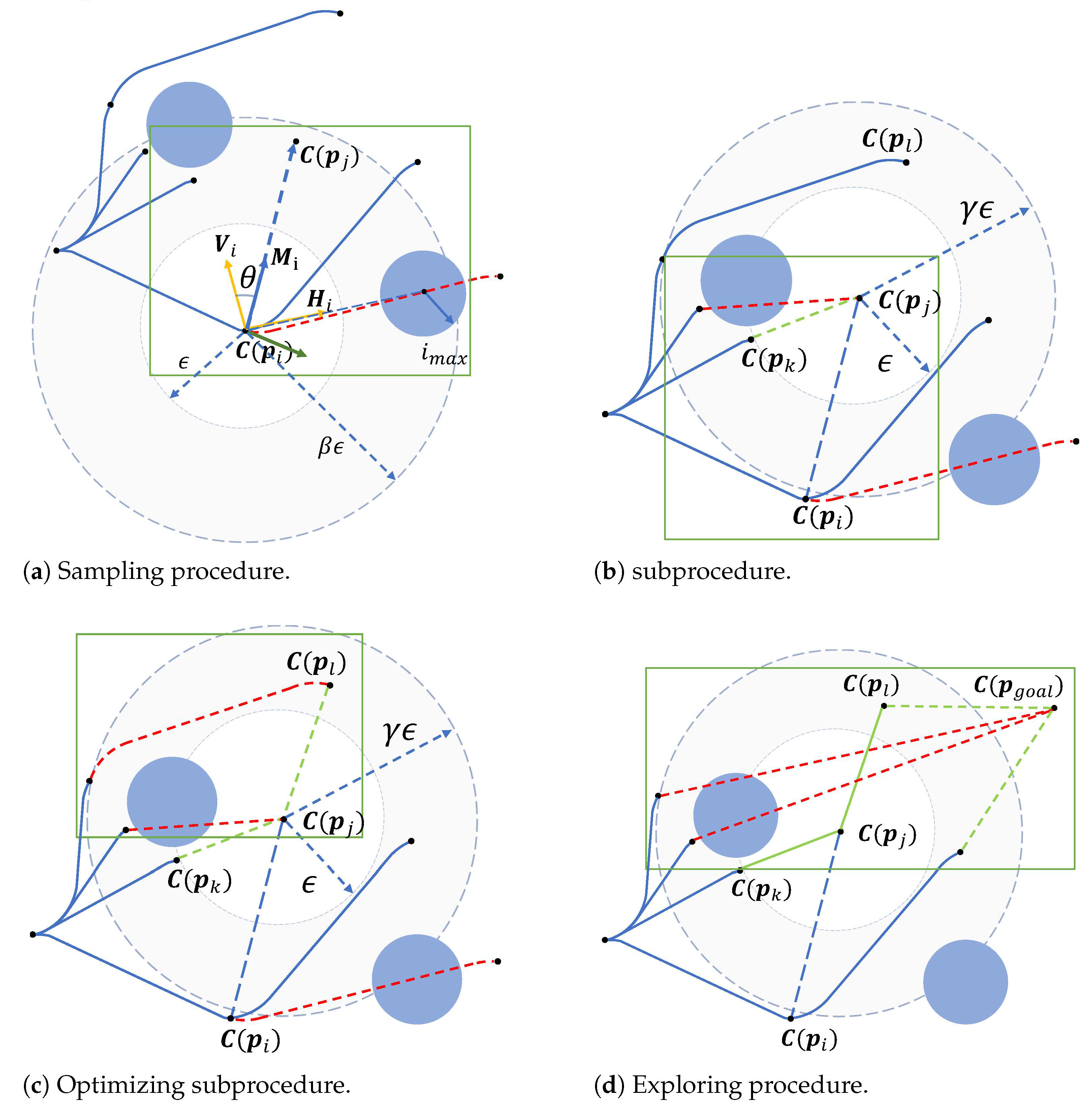
3.4.1. Sampling in Obstructive Environment

Sample nodes are generated corresponding to the nodes in $V_{new}$, as illustrated in Figure 6.

For each node $\mathcal{C}\left({\mathbf{p}}_j\right)\in V_{new}$, a new sample node is generated along a direction $\mathbf{M}\left({\mathbf{p}}_j\right)$, which is pseudorandomly determined based on two unit vectors $\mathbf{H}\left({\mathbf{p}}_j\right)$ and $\mathbf{V}\left({\mathbf{p}}_j\right)$. The vector $\mathbf{H}\left({\mathbf{p}}_j\right)$ indicates the forward direction towards the destination and is defined as $\mathbf{H}\left({\mathbf{p}}_j\right)=\mathbf{n}\left({\mathbf{o}}_{i_{max}}\left(t_{maxc}\right)-{\mathbf{p}}_j\right)$.

Meanwhile, $\mathbf{V}\left({\mathbf{p}}_j\right)$ represents the direction away from the original path $\mathbf{L}$ to help avoid collisions, and it is calculated as $\mathbf{V}\left({\mathbf{p}}_j\right)=\mathbf{n}(\mathbf{H}\left({\mathbf{p}}_j\right)\times {\mathbf{V}}_{\mathrm{rand}})$, where ${\mathbf{V}}_{\mathrm{rand}}\in {\mathbb{R}}^3$ is a randomly generated unit vector.

Then, the sampling direction $\mathbf{M}\left({\mathbf{p}}_j\right)$ is determined by a pseudorandom linear combination of $\mathbf{H}\left({\mathbf{p}}_j\right)$ and $\mathbf{V}\left({\mathbf{p}}_j\right)$ as

$$\mathbf{M}\left({\mathbf{p}}_j\right)=\mathbf{n}\left(sin\theta \mathbf{H}\left({\mathbf{p}}_j\right)+cos\theta \mathbf{V}\left({\mathbf{p}}_j\right)\right),$$

(13)

where $\theta$ denotes the clockwise angle from $\mathbf{V}\left({\mathbf{p}}_j\right)$ to $\mathbf{M}\left({\mathbf{p}}_j\right)$ and is generated by $\theta =2\pi (w^{\alpha }-0.5)$ with $w\in [0,1]$ being a uniform random variable and $\alpha \in [0,1]$ a shaping parameter. A random steering distance ${\Delta }_{\mathrm{new}}$ is then sampled from the interval $[ϵ,\beta ϵ]$, where $ϵ=4r_{\min }$ and $\beta \ge 1$. Accordingly, the new sample node $\mathcal{C}\left({\mathbf{p}}_{\mathrm{new}}\right)$ is generated at the position ${\mathbf{p}}_j+{\Delta }_{\mathrm{new}}·\mathbf{M}\left({\mathbf{p}}_j\right)$.

To ensure both the validity and efficiency of the sampling process, the spatio-temporal feasibility of the connection between the newly generated node $\mathcal{C}\left(\mathbf{p}\mathrm{new}\right)$ and its nearest existing node $\mathcal{C}\left(\mathbf{p}\mathrm{nst}\right)\in \mathcal{G}$ is evaluated using a linear uniform motion model to approximate the UUV trajectory.

The candidate path from $\mathcal{C}\left(\mathbf{p}\mathrm{nst}\right)$ to $\mathcal{C}\left(\mathbf{p}\mathrm{new}\right)$ is denoted as $\mathcal{D}\mathrm{nst},\mathrm{new}$, and its traversal cost is estimated by $\widehat{T}(\mathbf{p}\mathrm{nst},\mathbf{p}\mathrm{new})$. The configuration vector $\mathcal{V}\left(\mathbf{p}\mathrm{new}\right)$ is then updated according to the following rule

$$\mathcal{V}\left({\mathbf{p}}_{new}\right)=\mathbf{n}\left(\mathbf{n}\left({\mathbf{p}}_{new}-{\mathbf{p}}_{nst}\right)+\mathbf{n}\left({\mathbf{p}}_{goal}-{\mathbf{p}}_{new}\right)\right)$$

(14)

If the path ${\mathcal{D}}_{\mathrm{nst},\mathrm{new}}$ is collision-free, the parent node of $\mathcal{C}\left({\mathbf{p}}_{\mathrm{new}}\right)$ is set to $\mathcal{C}\left({\mathbf{p}}_{\mathrm{nst}}\right)$, i.e., $\mathcal{F}\left({\mathbf{p}}_{\mathrm{new}}\right)=\mathcal{C}\left({\mathbf{p}}_{\mathrm{nst}}\right)$. Otherwise, the node $\mathcal{C}\left({\mathbf{p}}_{\mathrm{new}}\right)$ is discarded, and the sampling process is repeated.

In addition, the inefficiency of sampling in highly obstructed environments is also addressed. This issue arises when numerous sampling attempts fail to produce any feasible node, for instance, when a node $\mathcal{C}\left({\mathbf{p}}_j\right)$ is located too close to surrounding obstacles. To mitigate this problem, a maximum sampling attempt threshold $\eta$ is introduced. If more than $\eta$ consecutive invalid sample nodes are generated based on a specific node in $V_{\mathrm{new}}$, that node will be replaced by its parent node within $V_{\mathrm{new}}$ to guide further sampling in a more promising direction.

The detailed procedure of the sampling strategy is summarized in Algorithm 2.

Algorithm 2: Sampling procedure

1: $iter\leftarrow 0$ 2: while  $iter\le \eta$  do 3:    $iter\leftarrow iter+1$ 4:    calculate $\mathbf{M}\left({\mathbf{p}}_j\right)$ and ${\Delta }_{new}$ according to $\mathcal{C}\left({\mathbf{p}}_j\right)$ 5:    ${\mathbf{p}}_{new}\leftarrow {\mathbf{p}}_j+{\Delta }_{new}\mathbf{M}\left({\mathbf{p}}_j\right)$ 6:    ${\mathbf{p}}_{nst}\leftarrow \underset{\mathbf{p}\in \mathcal{G}}{argmin}\parallel \mathbf{p}-{\mathbf{p}}_{new}\parallel$ 7:    if ${\mathcal{D}}_{nst,new}$ is collision-free then 8:      remove $\mathcal{C}\left({\mathbf{p}}_j\right)$ from $V_{open}$ 9:      break 10:    end if 11: end while 12: if $\mathcal{C}\left({\mathbf{p}}_{new}\right)$ is valid then 13:    remove $\mathcal{C}\left({\mathbf{p}}_j\right)$ from $V_{open}$ and $\mathcal{G}$ 14:    add $\mathcal{F}\left({\mathbf{p}}_j\right)$ to $V_{open}$ 15: end if

3.4.2. Expanding via Updating and Optimizing

The expanding procedure consists of two key components as follows: the updating subprocedure and the optimizing subprocedure, as illustrated in Figure 6b and Figure 6c, respectively.

In the updating subprocedure, the newly generated node $\mathcal{C}\left({\mathbf{p}}_{\mathrm{new}}\right)$ is connected to a node in $\mathcal{G}$ that minimizes the total cost to reach it. A set of nearby, reachable nodes in $\mathcal{G}$ is identified and recorded as $\left\{{\mathcal{C}}_{\mathrm{near}}\right\}$, where the Euclidean distance satisfies $\parallel {\mathcal{D}}_{\mathrm{near},\mathrm{new}}\parallel \in \left[ϵ,\gamma ϵ\right]$. The parameter $\gamma$ is defined as follows:

$$\gamma =max\left[1+{\left(\zeta \left(log\left(N_{\mathcal{G}}\right)\right)/N_{\mathcal{G}}\right)}^{1/\epsilon },\beta \right],$$

(15)

where $N_{\mathcal{G}}$ denotes the number of nodes in $\mathcal{G}$, $N_{\mathrm{obs}}$ is the number of detected obstacles, and $\zeta =\parallel {\mathcal{D}}_{\mathrm{new},\mathrm{goal}}{\parallel }^3/{\sum }_{i=1}^{N_{\mathrm{obs}}}{r}_i^3$. Among the nearby nodes, $\mathcal{C}\left({\mathbf{p}}_k\right)\in \left\{{\mathcal{C}}_{\mathrm{near}}\right\}$ is selected such that the total estimated cost $t\left({\mathbf{p}}_{\mathrm{new}}\right)$ is minimized

$$t\left({\mathbf{p}}_{new}\right)=t\left({\mathbf{p}}_k\right)+{\widehat{\mathrm{T}}}_{k,new}$$

(16)

where ${\widehat{\mathrm{T}}}_{k,\mathrm{new}}$ is the estimated transfer cost from $\mathcal{C}\left({\mathbf{p}}_k\right)$ to $\mathcal{C}\left({\mathbf{p}}_{\mathrm{new}}\right)$, and $\mathcal{V}\left({\mathbf{p}}_{\mathrm{new}}\right)$ is configured based on Equation (14).

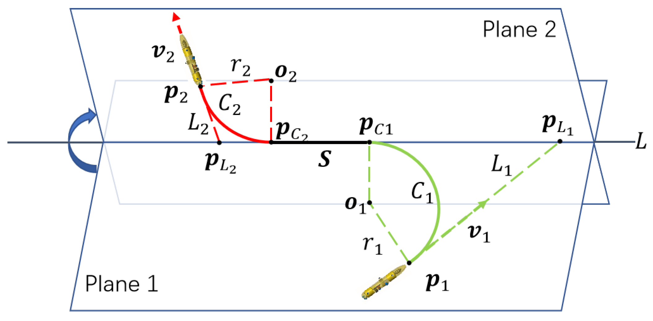
In conventional RRT*, the cost between two nodes is typically evaluated using Euclidean distance. However, such a metric fails to capture the actual traversal cost for nonholonomic vehicles like UUVs. To address this, the proposed method integrates 3D Dubins curve geometry into the tree-building process by replacing the Euclidean cost with an estimated Dubins curve length, denoted as ${\widehat{\mathcal{T}}}_{k,\mathrm{new}}$.

Specifically, during the updating subprocedure, the parent node $\mathcal{C}\left({\mathbf{p}}_k\right)$ of the newly generated node $\mathcal{C}\left({\mathbf{p}}_{\mathrm{new}}\right)$ is selected by minimizing the accumulated Dubins-based cost as follows:

$$\mathcal{C}\left({\mathbf{p}}_k\right)=arg\underset{{\mathbf{p}}_i\in \left\{{\mathcal{C}}_{\mathrm{near}}\right\}}{min}t\left({\mathbf{p}}_i\right)+{\widehat{\mathcal{T}}}_{i,\mathrm{new}},$$

(17)

where $t\left({\mathbf{p}}_i\right)$ denotes the cumulative cost from the root to node ${\mathbf{p}}_i$, and ${\widehat{\mathcal{T}}}_{i,\mathrm{new}}$ is the length of the Dubins curve estimated by the trained BPNN.

This formulation explicitly binds the Dubins curve geometry to the RRT* optimization process. The estimation ${\widehat{\mathcal{T}}}_{i,\mathrm{new}}$ captures both positional and directional constraints of the UUV, ensuring that path feasibility is evaluated under realistic kinematic assumptions. As a result, the tree growth is not only collision-aware but also curvature-constrained, leading to smoother and dynamically feasible trajectories.

Finally, the node $\mathcal{C}\left({\mathbf{p}}_{\mathrm{new}}\right)$ is added to $V_{\mathrm{new}}$, and the node $\mathcal{C}\left({\mathbf{p}}_k\right)$ is removed from $V_{\mathrm{open}}$ or $V_{\mathrm{new}}$ if it exists in either set.

In the optimizing subprocedure, the feasibility of the graph $\mathcal{G}$ is maintained by re-evaluating the connectivity of nearby nodes, as illustrated in Figure 6c. For each node $\mathcal{C}\left({\mathbf{p}}_l\right)\in \left\{{\mathcal{C}}_{\mathrm{near}}\right\}\setminus \mathcal{F}\left({\mathbf{p}}_{\mathrm{new}}\right)$, if the rough path ${\mathcal{R}}_{\mathrm{new},l}$ is both collision-free and results in a lower traversal cost compared to $t\left({\mathbf{p}}_l\right)$, then the parent of $\mathcal{C}\left({\mathbf{p}}_l\right)$ is updated to $\mathcal{C}\left({\mathbf{p}}_{\mathrm{new}}\right)$. Consequently, the cost is updated to $t\left({\mathbf{p}}_l\right)=t\left({\mathbf{p}}_{\mathrm{new}}\right)+{\widehat{\mathrm{T}}}_{\mathrm{new},l}$, the node $\mathcal{C}\left({\mathbf{p}}_l\right)$ is added to the re-evaluation set $V_{\mathrm{re}}$, and its new parent $\mathcal{F}\left({\mathbf{p}}_l\right)$ is stored in the reference set $V_{\mathrm{ref}}$.

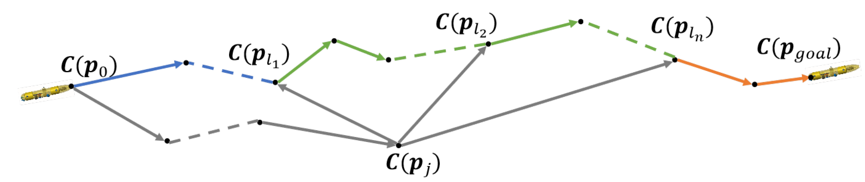
Changing the parent of a node may influence the spatio-temporal feasibility of its child nodes and may result in the derivation of new rough paths. For a rough path ${\mathcal{R}}_{r,e}$ comprising sequential nodes with updated parent relations, from ${\mathcal{C}}_{l_1}$ to ${\mathcal{C}}_{l_n}$, new rough paths may emerge in three distinct types, as illustrated in Figure 7.

The newly formed rough paths after parent update can be categorized into three types, illustrated in Figure 7, as follows:

Type I (blue solid lines): This path segment starts from the root node $\mathcal{C}\left({\mathbf{p}}_0\right)$ and ends at a parent-updated node ${\mathcal{C}}_{l_1}\in V_{\mathrm{ref}}$. It remains unchanged from the original path before optimization. The separation of this segment is caused by a change in the parent of ${\mathcal{C}}_{l_1}$, resulting in a disconnection between the former and latter parts of the path. Since it is a retained portion of a previously feasible path, its validity is preserved without requiring re-evaluation.

Type II (gray + green dashed lines): This path starts from the root node $\mathcal{C}\left({\mathbf{p}}_0\right)$, passes through a newly added node $\mathcal{C}\left({\mathbf{p}}_j\right)$ and a parent-updated node ${\mathcal{C}}_{l_1}$, and ends at the former parent of another updated node ${\mathcal{C}}_{l_2}$. The first segment (to $\mathcal{C}\left({\mathbf{p}}_j\right)$) is shown in gray, and the latter segment (original path portion) in green. This path arises when two or more nodes along the original path undergo parent updates, and a new path is formed by combining the prefix path to ${\mathcal{C}}_{l_1}$ with the suffix path from the parent of ${\mathcal{C}}_{l_2}$. Since the node costs are modified during this process, rechecking the feasibility of this path is necessary.

Type III (gray + orange dashed lines): This path starts at $\mathcal{C}\left({\mathbf{p}}_0\right)$, passes through a newly inserted node and a parent-updated node ${\mathcal{C}}_{l_n}$, and finally reaches the original goal $\mathcal{C}\left({\mathbf{p}}_{\mathrm{goal}}\right)$. The first segment (up to ${\mathcal{C}}_{l_n}$) is gray, and the last part (to the goal) is shown in orange. This type arises when the suffix of a path containing a parent-updated node is combined with the original goal-reaching segment. As the updated node costs differ from the original, feasibility verification is also required.

As highlighted in Remark 2, each new rough path has a one-to-one correspondence with an updated node in $V_{\mathrm{ref}}$. The validity of these new rough paths is verified in the subsequent step.

Candidate new paths are obtained by backtracking from nodes in the union set $V_{\mathrm{new}}\cup V_{\mathrm{open}}\cup V_{\mathrm{close}}\cup V_{\mathrm{ref}}$ toward the initial node $\mathcal{C}\left({\mathbf{p}}_0\right)$. To facilitate this process, three empty sets—$V_{\mathrm{new}}^{*}$, $V_{\mathrm{open}}^{*}$, and $V_{\mathrm{close}}^{*}$—are initialized. These sets serve as the updated counterparts of $V_{\mathrm{new}}$, $V_{\mathrm{open}}$, and $V_{\mathrm{close}}$, respectively, and they are used to store the new terminal nodes of $\mathcal{G}$ after the expansion procedure.

Paths that do not contain any nodes in $V_{\mathrm{re}}$ (i.e., paths unaffected by parent updates) are skipped, and their terminal nodes are directly transferred to the corresponding new sets. Only the paths that include parent-updated nodes in $V_{\mathrm{re}}$ are subject to further evaluation. Among these, collision-free paths are retained, and their terminal nodes are stored in the appropriate new sets accordingly. For infeasible paths, the unreachable segments are discarded, and the last valid node along each path is marked as the new terminal node and saved in $V_{\mathrm{new}}^{*}$.

Upon completion of this backtracking process, the spatio-temporal feasibility of $\mathcal{G}$ is guaranteed, and the updated terminal nodes are consistently tracked and maintained for subsequent planning stages. A pseudo code of the expanding procedure is presented in the Algorithm 3.

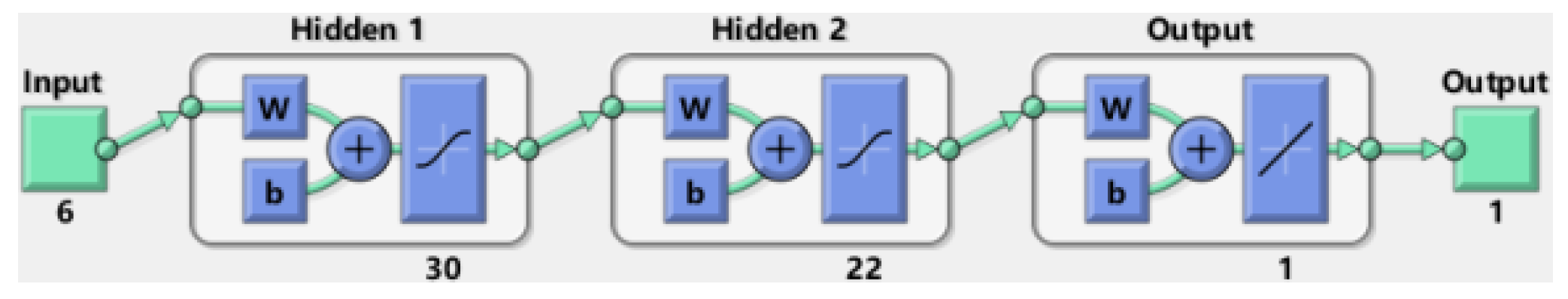
The BPNN model introduced in Section 2 is trained to efficiently estimate the Dubins curve length ${\widehat{\mathcal{T}}}_{i,j}$ between two 3D configurations. During RRT* tree expansion, these estimations are used as substitutes for analytically computed Dubins lengths, which are computationally expensive to evaluate at every iteration.

Algorithm 3: Expanding procedure

1: determine $\left\{{\mathcal{C}}_{near}\right\}$ 2: $\mathcal{C}\left({\mathbf{p}}_k\right)\leftarrow \underset{{\mathbf{p}}_i\in \left\{{\mathcal{C}}_{near}\right\}}{argmin}t\left(\mathbf{p}\right)+{\widehat{\mathrm{T}}}_{i,new}$ 3: $\mathcal{F}\left({\mathbf{p}}_{new}\right)\leftarrow \mathcal{C}\left({\mathbf{p}}_k\right)$, remove $\mathcal{C}\left({\mathbf{p}}_k\right)$ from $V_{open}\bigcup V_{new}$ 4: for  $\mathcal{C}\left({\mathbf{p}}_l\right)\in \left\{{\mathcal{C}}_{near}\right\}/\mathcal{C}\left({\mathbf{p}}_k\right)$do 5:    if ${\mathcal{D}}_{new,l}$ is collision-free and ${\mathcal{R}}_{new,l}$ is shorter then 6:      store $\mathcal{F}\left({\mathbf{p}}_l\right)$ in $V_{ref}$, $\mathcal{F}\left({\mathbf{p}}_l\right)\leftarrow \mathcal{C}\left({\mathbf{p}}_{new}\right)$ 7:       $t\left({\mathbf{p}}_l\right)\leftarrow t\left({\mathbf{p}}_{new}\right)+\widehat{\mathrm{T}}\left(new,l\right)$ 8:    end if 9: end for 10: for  $\mathcal{C}\left({\mathbf{p}}_{l_m}\right)\in V_{open}\cup V_{new}\cup V_{close}\cup V_{ref}$do 11:    backtracking from $\mathcal{C}\left({\mathbf{p}}_{l_m}\right)$ towards $\mathcal{C}\left({\mathbf{p}}_0\right)$ 12:    if ${\mathcal{R}}_{p,l_m}$ has no node in $V_{re}$ then 13:      if ${\mathcal{R}}_{p,l_m}$ is collision-free then 14:         move $\mathcal{C}\left({\mathbf{p}}_{l_m}\right)$ to $V_{open}^{*}$ 15:      else 16:         move the last reachable node to $V_{new}^{*}$ 17:      end if 18:    else 19:      if $\mathcal{C}\left({\mathbf{p}}_{l_m}\right)\in V_{open}\cup V_{new}\cup V_{close}$ then 20:         store $\mathcal{C}\left({\mathbf{p}}_{l_m}\right)$ correspondingly to the new set 21:      else 22:         store $\mathcal{C}\left({\mathbf{p}}_{l_m}\right)$ to $V_{open}^{*}$ 23:      end if 24:    end if 25: end for

By integrating the BPNN estimator into the cost function (Equation (17)), the parent selection process becomes both curvature-aware and computationally efficient. This significantly reduces the time complexity of each expansion step while maintaining path smoothness and feasibility. Nodes that would otherwise be chosen based on Euclidean distance are now selected based on a learned approximation of the true traversal cost under kinematic constraints.

Furthermore, the BPNN-estimated lengths guide the rewiring process and cost updates throughout the graph. As the BPNN captures geometric characteristics such as initial/final direction and curvature limits, it ensures that suboptimal parents (with low Euclidean cost but high curvature) are avoided. This results in smoother paths with fewer unnecessary turns or abrupt heading changes.

3.4.3. Exploring Towards Destination

The exploring procedure is designed to be goal-biased, and it operates based on the set $V_{\mathrm{open}}^{*}$ to derive a sufficient number of candidate rough paths, as illustrated in Figure 6d. For each node $\mathcal{C}\left({\mathbf{p}}_l\right)\in V{\mathrm{open}}^{*}$, the feasibility of the path ${\mathcal{R}}_{l,\mathrm{goal}}$ is evaluated.

If ${\mathcal{R}}_{l,\mathrm{goal}}$ is collision-free, it is considered a potentially feasible maneuver, and the corresponding node $\mathcal{C}\left({\mathbf{p}}_l\right)$ is moved to $V_{\mathrm{close}}^{*}$. Otherwise, if the path is found to be infeasible, further path planning for collision avoidance is required, and the node is instead moved to $V_{\mathrm{new}}^{*}$. To ensure a balance between path diversity (sufficiency) and computational tractability (efficiency), the exploring procedure incorporates two mature criteria to control the growth of the graph $\mathcal{G}$. Let $N_{V_{\mathrm{close}}}$ denote the number of nodes in $V_{\mathrm{close}}^{*}$. If $N_{V_{close}}$ denotes the number of the nodes in $V_{close}^{*}$, the mature criteria are expressed as

(1)

$N_{V_{\mathrm{close}}}$ exceeds a predefined positive threshold $\kappa$;

(2)

Both $V_{\mathrm{open}}^{*}$ and $V_{\mathrm{new}}^{*}$ are empty.

When either criterion is satisfied, $\mathcal{G}$ is considered to be sufficiently expanded, and the reshaping procedure is subsequently initiated. The pseudocode for the exploring procedure is presented in Algorithm 4.

Algorithm 4: Exploring procedure

1: for  $\mathcal{C}\left({\mathbf{p}}_l\right)\in V_{open}^{*}$  do 2:    if $N_{V_{close}}\le \kappa$ or $V_{open}^{*}\cup V_{new}^{*}\ne \varnothing$ then 3:      if ${\mathcal{R}}_{l,goal}$ is collision-free then 4:         remove $\mathcal{C}\left({\mathbf{p}}_l\right)$ from $V_{open}^{*}$ to $V_{close}^{*}$ 5:      else 6:         remove $\mathcal{C}\left({\mathbf{p}}_l\right)$ from $V_{open}^{*}$ to $V_{new}^{*}$ 7:      end if 8:    end if 9: end for

3.5. Path Reshape

Rather than reshaping each candidate rough path individually, the proposed method begins by comparing their costs with the current shortest smoothed path. Let $t_{min}$ denote the cost of the current shortest smooth path. For the shortest candidate rough path ${\mathcal{R}}_{m,\mathrm{goal}}$, if its cost is less than $t_{min}$, it is considered a promising candidate for further optimization.

The component nodes of ${\mathcal{R}}_{m,\mathrm{goal}}$, which are generated by the improved RRT* algorithm, are reconfigured and evaluated sequentially. For each node $\mathcal{C}\left({\mathbf{p}}_i\right)\in {\mathcal{R}}_{m,\mathrm{goal}}$, the configuration $\mathcal{V}\left({\mathbf{p}}_i\right)$ is redefined according to Equation (14) by substituting ${\mathbf{p}}_{\mathrm{goal}}$ with the position of its child node in ${\mathcal{R}}_{m,\mathrm{goal}}$.

Subsequently, a 3D Dubins curve is determined from the parent node $\mathcal{F}\left({\mathbf{p}}_i\right)$ to the current node $\mathcal{C}\left({\mathbf{p}}_i\right)$, and its feasibility is assessed. Let $\mathcal{C}\left({\mathbf{p}}_j\right)=\mathcal{F}\left({\mathbf{p}}_i\right)$. If the Dubins curve ${\mathcal{T}}_{j,i}$ is collision-free, the cost is updated as

$$t\left({\mathbf{p}}_i\right)=t\left({\mathbf{p}}_j\right)+{\mathcal{T}}_{j,i},$$

(18)

and the curve is stored accordingly.

If a collision is detected, the reshaping process for ${\mathcal{R}}_{m,\mathrm{goal}}$ is terminated, and the infeasible portion of the path—from $\mathcal{C}\left({\mathbf{p}}_i\right)$ to the terminal node $\mathcal{C}\left({\mathbf{p}}_f\right)$—is discarded. The collision detection result is also stored in correspondence with $\mathcal{F}\left({\mathbf{p}}_i\right)$ for further handling.

Finally, if the reshaped path ${\mathcal{L}}_{m,\mathrm{goal}}$ is entirely collision-free and its cost is less than $t_{min}$, then ${\mathcal{L}}_{m,\mathrm{goal}}$ is saved as the new optimal solution, and $t_{min}$ is updated accordingly. In addition, after processing all the candidate rough paths, the shortest smooth result, if it exists, is accepted as $\mathbf{L}$. If no feasible smooth path is determined, the improved RRT* algorithm will be repeated.

4. Simulation and Discussion

To prove the validity and efficiency of the smooth path planning method, comparative simulation results with state-of-the-art algorithms—3D RRT*, Informed RRT* [13], Stable Sparse RRT* (SST*) [25], Dynamic RRT* [26], and the asymptotically optimal single-query sampling-based replanning algorithm RRTX [27]—in unknown scenarios with static and moving obstacles are provided in this section.

For simplicity of expression, the proposed smooth path planning method is referred to as DRRT*. Its parameters are configured as presented in

Table 4. Parameter selection.

Parameter	$\mathit{\alpha }$	$\mathit{ϵ}$	$\mathit{\beta }$	$\mathit{\epsilon }$	$\mathit{\eta }$	$\mathit{\kappa }$
Value	$1/6$	$4r_{min}$	$1.5$	3	100	1

.

To ensure fairness, all algorithms employ the same collision detection function and share some common algorithmic parameters. In the comparative studies, the kinematic and dynamic constraints of the UUV are ignored for the 3D RRT*, Informed RRT*, and Dynamic RRT* algorithms. For these methods, 100 additional sample nodes are appended after each planning failure to ensure that a complete resultant path can be generated. The RRTX algorithm also ignores the prescribed constraints. However, its number of sample nodes is fixed at 800 to increase the probability of finding a goal-reachable path. In contrast, the SST* algorithm shares the same kinematic model as the proposed DRRT* method. Its initial number of sample nodes is set to 100. To complete the path planning task, Dubins curves are used to connect the random tree to the terminal configuration. Each algorithm is executed 50 times on a laptop equipped with an Intel i7-9750H CPU, 16GB RAM, and running MATLAB 2019b.

The parameters of the UUV are set as $r_{min}=1\mathrm{m}$ and $r_{scan}=7\mathrm{m}$, and the prescribed configurations are

$$\left\{\begin{array}{c}\mathbf{p}={[0\mathrm{m},0\mathrm{m},0\mathrm{m}]}^{\mathrm{T}},\hfill \\ \mathbf{v}={[1\mathrm{m}/\mathrm{s},0\mathrm{m}/\mathrm{s},0\mathrm{m}/\mathrm{s}]}^{\mathrm{T}},\hfill \end{array}\right.$$

(19)

and

$$\left\{\begin{array}{c}{\mathbf{p}}_{goal}={[20\mathrm{m},0\mathrm{m},0\mathrm{m}]}^{\mathrm{T}},\hfill \\ \mathcal{V}\left({\mathbf{p}}_{goal}\right)={[1\mathrm{m}/\mathrm{s},0\mathrm{m}/\mathrm{s},0\mathrm{m}/\mathrm{s}]}^{\mathrm{T}}.\hfill \end{array}\right.$$

(20)

4.1. Scenario 1: Unknown Environment with Static Obstacles

In this scenario, 22 unknown obstacles form a concave obstructive area. The simulation results of the compared algorithms are shown in Figure 8. Figure 8f illustrates the path planning result of the proposed DRRT*, demonstrating its capability to effectively avoid the concave obstruction and generate a feasible, smooth maneuver to reach the goal configuration.

Compared to the other algorithms shown in Figure 8, the path generated by DRRT* exhibits improved smoothness. The average curvature computed over 10 randomized trials is $0.35$, $0.23$, $0.22$, $0.18$, and $0.20$ ${\mathrm{m}}^{-1}$ for 3D RRT*, informed RRT*, Dynamic RRT*, SST*, and RRTX, respectively, while DRRT* yields the lowest average curvature of $0.16$ ${\mathrm{m}}^{-1}$.

The statistical performance of DRRT* and the comparative methods in this scenario is further summarized in Figure 9. Figure 9a presents the path length statistics, where the average lengths of the resultant paths generated by 3D RRT*, informed RRT*, Dynamic RRT*, SST*, and RRTX are $43.60\mathrm{m}$, $57.88\mathrm{m}$, $49.68\mathrm{m}$, $46.48\mathrm{m}$, and $40.54\mathrm{m}$, respectively. In contrast, the average path length obtained by DRRT* is only $26.71\mathrm{m}$. Meanwhile, the computational time consumption of these algorithms is shown in Figure 9b. The average time taken by 3D RRT*, informed RRT*, Dynamic RRT*, SST*, and RRTX to generate collision-free paths is $5.54\mathrm{s}$, $2.15\mathrm{s}$, $3.83\mathrm{s}$, $145.03\mathrm{s}$, and $4.21\mathrm{s}$, respectively. In comparison, DRRT* achieves superior efficiency, requiring only $1.54\mathrm{s}$ on average.

4.2. Scenario 2: An Unknown Environment with Both Static and Moving Obstacles

Scenario 2 represents an unknown environment populated with 16 static obstacles and 4 moving obstacles. These obstacles are randomly distributed, and the moving obstacles travel at a constant speed of $1\mathrm{m}/\mathrm{s}$.

The simulation results of the path planning algorithms are illustrated in Figure 10. Specifically, Figure 10f shows the path generated by the proposed DRRT* algorithm. Compared to the results of the other algorithms shown in Figure 10, DRRT* produces a smooth and collision-free trajectory that successfully reaches the goal configuration.

A statistical comparison of the algorithms’ performance in this scenario is provided in Figure 11. Figure 11a presents the lengths of the resulting paths. The average path lengths for the 3D RRT*, informed RRT*, Dynamic RRT*, SST*, and RRTX algorithms are $42.2141\mathrm{m}$, $54.6791\mathrm{m}$, $40.2476\mathrm{m}$, $47.5439\mathrm{m}$, and $37.0687\mathrm{m}$, respectively. In contrast, DRRT* achieves a significantly shorter average path length of $23.2824\mathrm{m}$.

The computational cost of each algorithm is compared in Figure 11b. On average, the 3D RRT*, informed RRT*, Dynamic RRT*, SST*, and RRTX algorithms require $3.7574\mathrm{s}$, $2.0170\mathrm{s}$, $3.1541\mathrm{s}$, $81.6918\mathrm{s}$, and $4.0694\mathrm{s}$, respectively, to generate a complete collision-free path. In comparison, DRRT* demonstrates superior efficiency, completing the planning task in an average of only $1.3029\mathrm{s}$.

4.3. Scenario 3: Evaluating Robustness in a High-Density Obstacle Environment

To rigorously evaluate the effectiveness and robustness of the proposed DRRT* algorithm under more demanding environmental conditions, Scenario 3 introduces a significantly more complex test case. This scenario features an expanded workspace and a substantially increased density of obstacles compared to Scenarios 1 and 2, specifically designed to assess the algorithm’s performance in settings representative of challenging real-world navigation tasks.

Within this environment, the spatial dimensions are increased, and both static and moving obstacles are densely distributed to create a highly constrained planning problem with active dynamic hazards. The obstacle configuration builds upon the principles established in Scenario 1, but incorporates additional dynamic obstacles exhibiting complex converging and diverging movement patterns to further test the algorithm’s ability to handle intricate interactions. We also include traditional methods such as APF and modified RRT in this scenario to provide a broader baseline reference, especially under highly constrained and dynamic conditions.

The simulation results for all tested algorithms are presented in Figure 12. As Figure 12h illustrates, the DRRT* algorithm successfully computes a smooth and collision-free trajectory, effectively navigating the dense static obstacles and dynamically avoiding the moving hazards.

Statistical performance metrics for this scenario are summarized in Figure 13 and

Table 5. Simulation results in Scenario 3.

Algorithm	Item	Length	Nodes Num	Time Consumption
APF	Max	$32.50$	−	$0.13$ s
	Aver	$31.14$	−	$0.10$ s
	Min	$30.60$	−	$0.09$ s
Modified RRT*	Max	$42.99$	569	$221.31$ s
	Aver	$31.97$	$235.45$	$59.31$ s
	Min	$23.52$	82	$10.97$ s
DRRT*	Max	$39.10$	86	$6.93$ s
	Aver	$26.94$	$18.83$	$1.42$ s
	Min	$22.40$	4	$0.16$ s

. Figure 13a shows that DRRT* achieves the shortest average path length of $26.94\mathrm{m}$, while also demonstrating the lowest average computation time of $1.42\mathrm{s}$ (Figure 13b). Table 5 further confirms DRRT’s superior success rate and overall efficiency when compared to traditional APF and modified RRT-based planners.

These results demonstrate that DRRT* maintains its significant performance advantages even in moderately scaled environments characterized by high obstacle density and complex dynamic interactions, highlighting its enhanced robustness. However, the current framework’s performance boundaries are noted: scenarios involving extremely large−scale underwater domains (e.g., $>1000\mathrm{m}$ range) or exceptionally high numbers of obstacles (e.g., $>200$) may challenge its efficiency due to increased memory requirements and sampling complexity, potentially impacting runtime and success rates. Exploring extensions to handle such extreme scales will be the focus of future work.

4.4. Discussion on Scalability and Limitations

Although the proposed DRRT* algorithm demonstrates significant performance improvements in the tested scenarios, it is important to acknowledge the current limitations regarding environmental complexity. The simulation environments primarily involve moderate obstacle densities and confined spatial regions. As obstacle density increases or the environment size expands, several challenges may arise, including increased sampling requirements, higher memory consumption, and longer convergence times.

However, due to the modular structure of the proposed method—including fast Dubins estimation, goal−biased exploration, and partial path reuse—it is inherently scalable. In larger−scale environments, planning performance can be maintained by increasing the sampling budget or employing adaptive pruning strategies. These extensions, along with quantitative evaluations in dense and cluttered environments (e.g., $200+$ obstacles over $1000\mathrm{m}$ scale), are left as future work.

5. Conclusions

In this paper, we addressed the path planning problem for a nonholonomic UUV operating in unknown 3D environments with obstacles. An efficient and smooth path planning approach was proposed by integrating 3D Dubins curves with an enhanced version of the RRT* algorithm. We analyzed the geometric characteristics of 3D Dubins curves and introduced a rapid curve length estimation method based on a backpropagation (BP) neural network. To improve the efficiency of the planning algorithm, several modifications were made to the original RRT*, including pseudorandom sampling, terminal−node backtracking−based extension, and goal−biased exploration. These enhancements significantly reduce computational overhead and improve the algorithm’s collision avoidance capability. Comprehensive simulation experiments validated the effectiveness and feasibility of the proposed method in unknown environments. Future work will focus on integrating this smooth path planning framework with advanced perception systems and robust controllers to further enhance the mobility and adaptability of the UUVs in complex, unstructured outdoor scenarios.

References

1. Wu, B.; Yan, X.; Wang, Y.; Guedes Soares, C. An evidential reasoning-based CREAM to human reliability analysis in maritime accident process. Risk Anal. 2017, 37, 1936–1957. [Google Scholar] [CrossRef]
2. Chen, X.; Wei, C.; Xin, Z.; Zhao, J.; Xian, J. Ship detection under low-visibility weather interference via an ensemble generative adversarial network. J. Mar. Sci. Eng. 2023, 11, 2065. [Google Scholar] [CrossRef]
3. Wang, H.; Gao, W.; Wang, Z.; Zhang, K.; Ren, J.; Deng, L.; He, S. Research on Obstacle Avoidance Planning for UUV Based on A3C Algorithm. J. Mar. Sci. Eng. 2024, 12, 142–149. [Google Scholar] [CrossRef]
4. Zhang, T.; Li, Q.; Zhang, C.; Liang, H.; Li, P.; Wang, T.; Li, S.; Zhu, Y.; Wu, C. Current trends in the development of intelligent unmanned autonomous systems. Front. Inf. Technol. Electron. Eng. 2017, 18, 68–85. [Google Scholar] [CrossRef]
5. Cui, R.; Yang, C.; Li, Y.; Sharma, S. Adaptive Neural Network Control of AUVs With Control Input Nonlinearities Using Reinforcement Learning. IEEE Trans. Syst. Man Cybern. Syst. 2017, 47, 1019–1029. [Google Scholar] [CrossRef]
6. Zhang, X.; Wang, Z.; Chen, H.; Ding, H. A Trajectory Tracking and Local Path Planning Control Strategy for Unmanned Underwater Vehicles. J. Mar. Sci. Eng. 2023, 11, 2230. [Google Scholar] [CrossRef]
7. Mac, T.T.; Copot, C.; Tran, D.T.; De Keyser, R. Heuristic approaches in robot path planning: A survey. Robot. Auton. Syst. 2016, 86, 13–28. [Google Scholar] [CrossRef]
8. Luis Sanchez-Lopez, J.; Wang, M.; Olivares-Mendez, M.A.; Molina, M.; Voos, H. A Real-Time 3D Path Planning Solution for Collision-Free Navigation of Multirotor Aerial Robots in Dynamic Environments. J. Intell. Robot. Syst. 2019, 93, 33–53. [Google Scholar] [CrossRef]
9. Mobadersany, P.; Khanmohammadi, S.; Ghaemi, S. A fuzzy multi-stage path-planning method for a robot in a dynamic environment with unknown moving obstacles. Robotica 2015, 33, 1869–1885. [Google Scholar] [CrossRef]
10. Liu, S.; Watterson, M.; Mohta, K.; Sun, K.; Bhattacharya, S.; Taylor, C.J.; Kumar, V. Planning Dynamically Feasible Trajectories for Quadrotors Using Safe Flight Corridors in 3-D Complex Environments. IEEE Robot. Autom. Lett. 2017, 2, 1688–1695. [Google Scholar] [CrossRef]
11. Karaman, S.; Frazzoli, E. Sampling-based algorithms for optimal motion planning. Int. J. Robot. Res. 2011, 30, 846–894. [Google Scholar] [CrossRef]
12. Webb, D.J.; van den Berg, J. Kinodynamic RRT*: Asymptotically optimal motion planning for robots with linear dynamics. In Proceedings of the 2013 IEEE International Conference on Robotics and Automation (ICRA), Karlsruhe, Germany, 6–10 May 2013; pp. 5054–5061. [Google Scholar]
13. Gammell, J.D.; Srinivasa, S.S.; Barfoot, T.D. Informed RRT*: Optimal sampling-based path planning focused via direct sampling of an admissible ellipsoidal heuristic. In Proceedings of the 2014 IEEE/RSJ International Conference on Intelligent Robots and Systems (IROS), Chicago, IL, USA, 14–18 September 2014; pp. 2997–3004. [Google Scholar]
14. Jian, X.; Zou, T.; Vardy, A.; Bose, N. A Hybrid Path Planning Strategy of Autonomous Underwater Vehicles. In Proceedings of the 2020 IEEE/OES Autonomous Underwater Vehicles Symposium (AUV), St. Johns, NL, Canada, 30 September 2020–2 October 2020; pp. 1–6. [Google Scholar]
15. Lee, H.; Kim, H.; Kim, H.J. Planning and Control for Collision-Free Cooperative Aerial Transportation. IEEE Trans. Autom. Sci. Eng. 2018, 15, 189–201. [Google Scholar] [CrossRef]
16. Qiao, W.; Fang, Z.; Si, B. Sample-based Frontier Detection for Autonomous Robot Exploration. In Proceedings of the 2018 IEEE International Conference on Robotics and Biomimetics (ROBIO), Kuala Lumpur, Malaysia, 12–15 December 2018; pp. 1165–1170. [Google Scholar]
17. Zhang, Z.; Wu, D.; Gu, J.; Li, F. A Path-Planning Strategy for Unmanned Surface Vehicles Based on an Adaptive Hybrid Dynamic Stepsize and Target Attractive Force-RRT Algorithm. J. Mar. Sci. Eng. 2019, 7, 132. [Google Scholar] [CrossRef]
18. Behandish, M.; Ilieş, H.T. Analytic methods for geometric modeling via spherical decomposition. Comput. Aided Des. 2016, 70, 100–115. [Google Scholar] [CrossRef]
19. Setty, S.; Mudenagudi, U. Example-based 3D inpainting of point clouds using metric tensor and Christoffel symbols. Mach. Vis. Appl. 2018, 29, 329–343. [Google Scholar] [CrossRef]
20. Kaya, C.Y. Markov-Dubins path via optimal control theory. Comput. Optim. Appl. 2017, 68, 719–747. [Google Scholar] [CrossRef]
21. Furtuna, A.A.; Balkcom, D.J. Generalizing Dubins Curves: Minimum-time Sequences of Body-fixed Rotations and Translations in the Plane. Int. J. Robot. Res. 2010, 29, 703–726. [Google Scholar] [CrossRef]
22. Tokekar, P.; Karnad, N.; Isler, V. Energy-optimal trajectory planning for car-like robots. Auton. Robot. 2014, 37, 279–300. [Google Scholar] [CrossRef]
23. Wehbe, B.; Bazzi, S.; Shammas, E. Novel three-dimensional optimal path planning method for vehicles with constrained pitch and yaw. Robotica 2017, 35, 2157–2176. [Google Scholar] [CrossRef]
24. Shkel, A.M.; Lumelsky, V. Classification of the Dubins set. Robot. Auton. Syst. 2001, 34, 179–202. [Google Scholar] [CrossRef]
25. Li, Y.; Littlefield, Z.; Bekris, K.E. Asymptotically optimal sampling-based kinodynamic planning. Int. J. Robot. Res. 2016, 35, 528–564. [Google Scholar] [CrossRef]
26. Connell, D.; La, H.M. Extended rapidly exploring random tree-based dynamic path planning and replanning for mobile robots. Int. J. Adv. Robot. Syst. 2018, 15, 1729881418773874. [Google Scholar] [CrossRef]
27. Otte, M.; Frazzoli, E. RRTX: Asymptotically optimal single-query sampling-based motion planning with quick replanning. Int. J. Robot. Res. 2016, 35, 797–822. [Google Scholar] [CrossRef]
Figure 1. Illustration of the 3D CSC Dubins curve. This curve is composed of two circular segments ( C 1 and C 2 ) and one straight line segment (S). The initial and terminal configurations of this curve are illustrated by green vector and red vector separately.
Jmse 13 01354 g001
Figure 2. Structure of the designed BPNN for length estimation.
Jmse 13 01354 g002
Figure 3. Error graph of the test result of Group 2. The blue bars represent the absolute estimation error of Dubins path lengths across 1000 samples. Red dots indicate outliers with the largest absolute errors. The inset zooms into the first 100 data points for local detail.
Jmse 13 01354 g003
Figure 4. Estimated and computed Dubins path lengths over 1000 random samples per group.
Jmse 13 01354 g004
Figure 5. Implementation of the proposed planning method triggered by changes in the feasibility of the current trajectory followed by the UUV.
Jmse 13 01354 g005
Figure 6. Illustration of the sampling, updating, optimizing, and exploring procedures: (a) Sampling direction generation and new node creation; (b) connection to the parent node with minimum cost; (c) cost optimization by reconnecting neighbors; (d) goal-biased exploration and rough path generation.
Jmse 13 01354 g006
Figure 7. Illustration of the three types of newly generated rough paths caused by parent updates during graph optimization. Type I (blue solid line): unchanged segment from the root node to a parent-updated node. Type II (gray + green dashed line): path connecting two updated nodes, combining a new segment with a reused part of the original path. Type III (gray + orange dashed line): updated segment from the root to an intermediate node, followed by the original goal-reaching portion.
Jmse 13 01354 g007
Figure 8. The typical simulation results of the comparative algorithms in Scenario 1. (a) Resultant path of 3D RRT*. (b) Resultant path of informed RRT*. (c) Resultant path of dynamic RRT*. (d) Resultant path of SST*. (e) Resultant path of RRTX. (f) Resultant path of DRRT*. In each subfigure, the blue line denotes the final path generated by the corresponding algorithm. The red short line marks the starting position, and the green sphere indicates the goal location. Colored segments such as yellow, red, or green represent intermediate path segments or exploration trajectories during planning. Obstacles are visualized as translucent blue and green spheres.
Jmse 13 01354 g008
Figure 9. Statistic results of path planning in Scenario 1. (a) The statistics of resultant path lengths in Scenario 1. (b) The statistics of computation consumptions in Scenario 1.
Jmse 13 01354 g009
Figure 10. The typical simulation results of the comparative algorithms in Scenario 2. (a) Resultant path of the 3D RRT*. (b) Resultant path of the informed RRT*. (c) Resultant path of the dynamic RRT*. (d) Resultant path of the SST*. (e) Resultant path of the RRTX. (f) Resultant path of the DRRT*. In each subfigure, the blue line denotes the final path generated by the corresponding algorithm. The red short line marks the starting position, and the green sphere indicates the goal location. Colored segments such as yellow, red, or green represent intermediate path segments or exploration trajectories during planning. Obstacles are visualized as translucent blue and green spheres.
Jmse 13 01354 g010
Figure 11. Statistic results of path planning in Scenario 2. (a) Statistics of resultant path lengths in Scenario 2. (b) Statistics of computation consumption in Scenario 2.
Jmse 13 01354 g011
Figure 12. Path planning results of the APF, Modified RRT*, and DRRT* algorithms in Scenario 3. (a) Local minimum problem in the APF algorithm. (b) Resultant path of the APF algorithm. (c) Initial path planning result of modified RRT*. (d) Path replanning result of modified RRT*. (e) Resultant path of modified RRT*. (f) Initial path planning result of DRRT*. (g) Path replanning result of DRRT*.
Jmse 13 01354 g012
Figure 13. Statistical comparison of the 3D RRT* and DRRT* algorithms in Scenario 3. (a) Path planning time consumption of the prescribed algorithms. (b) Resultant path length of the prescribed algorithms.
Jmse 13 01354 g013