
Underwater Target Localization Method Based on Uniform Linear Electrode Array

 ,
,  , , and
Abstract
1. Introduction
2. MUSIC Method
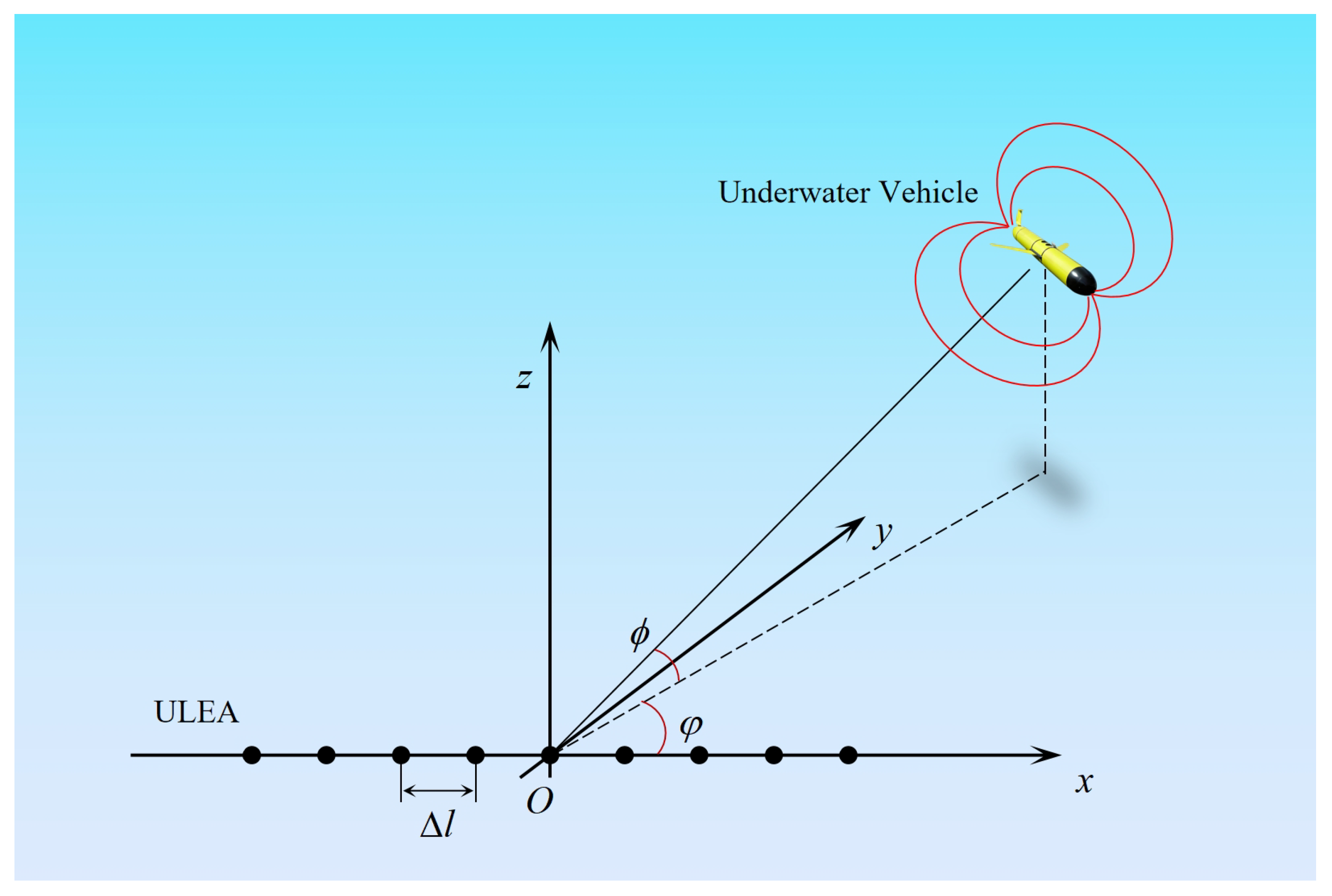
2.1. Locating System
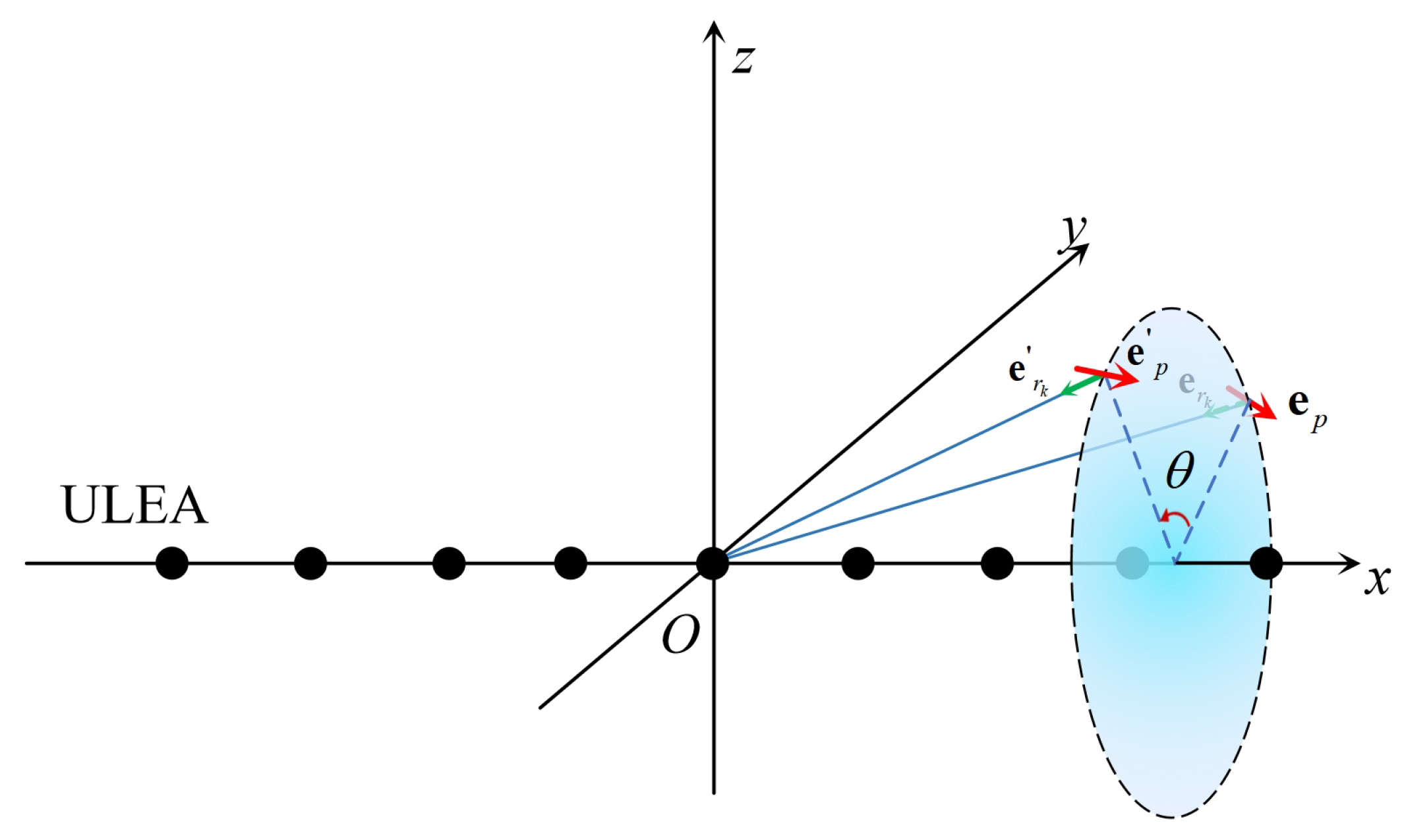
2.2. Array Manifold
2.3. Spatial Spectrum
2.4. Reducing the Calculation
| Algorithm 1: Underwater electric sources locating method based on ULEA |
Data: The ULEA received signal
Result: locations , ⋯, |
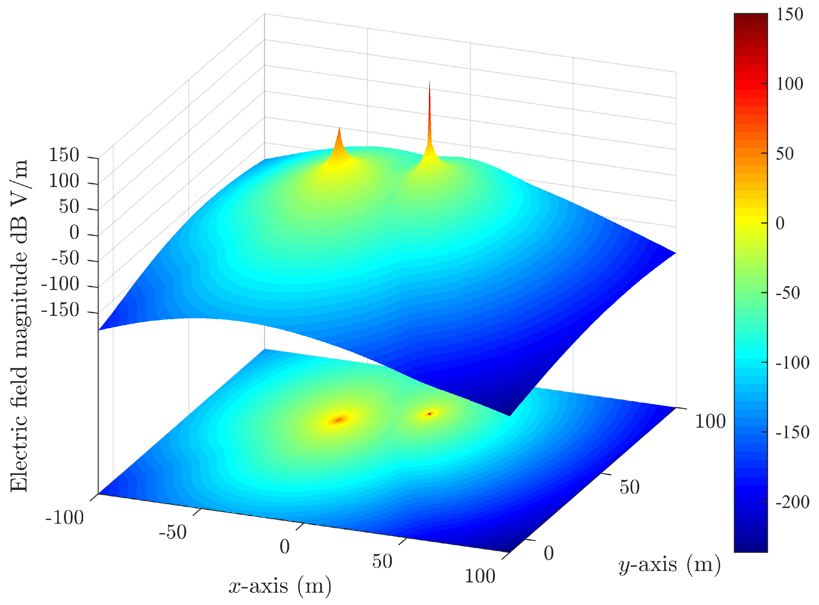
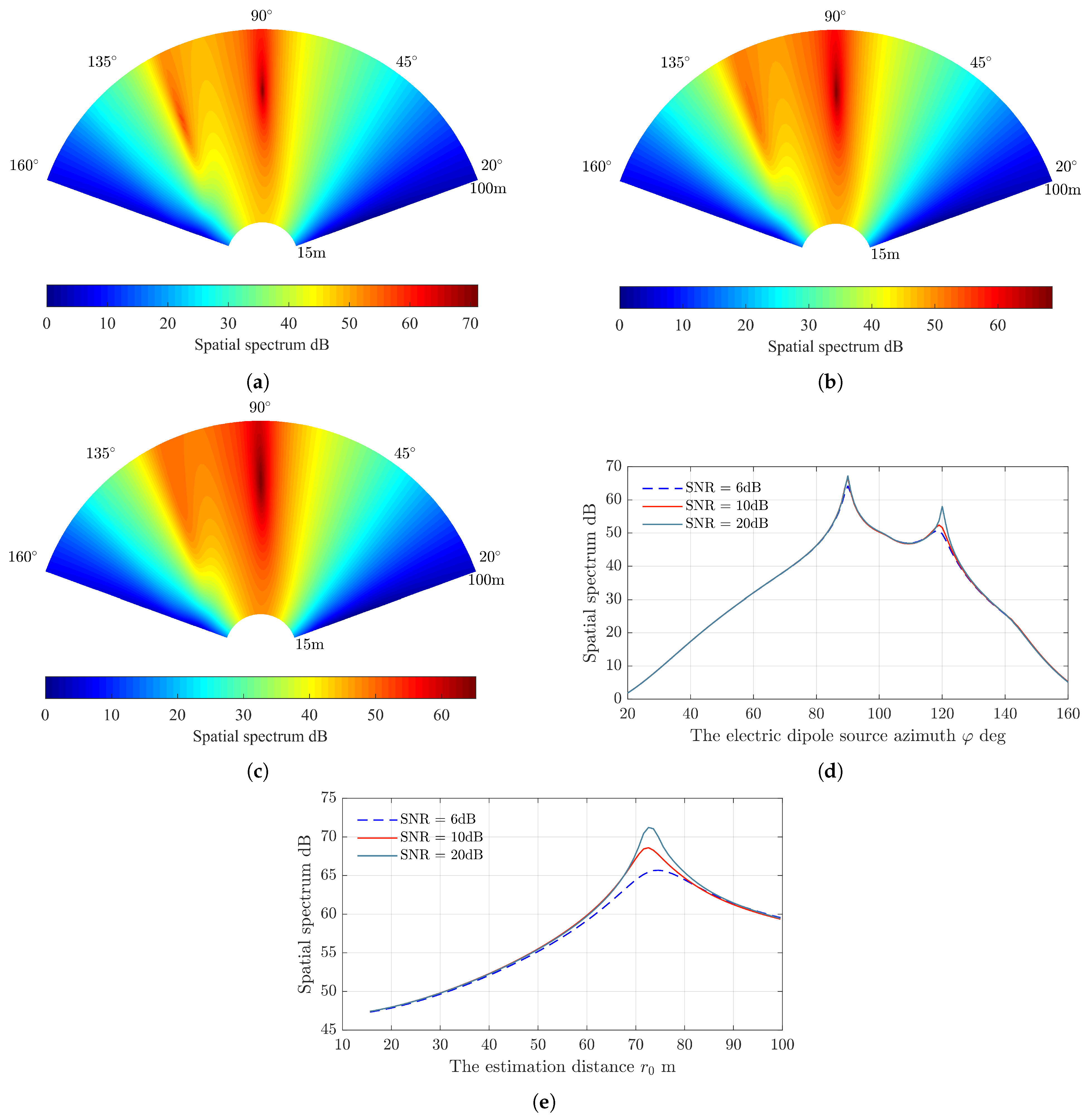
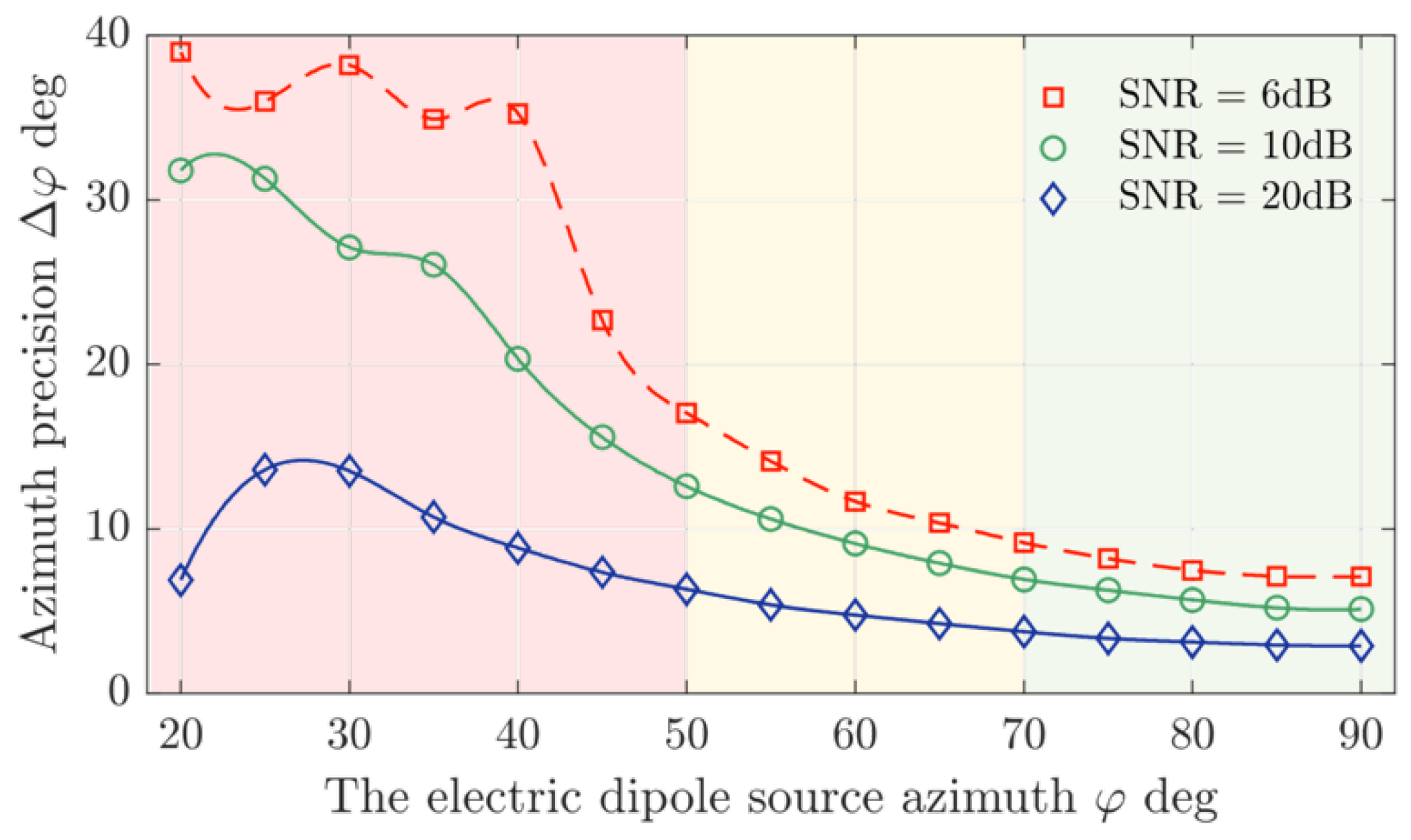
3. Simulation
4. Performance Analysis
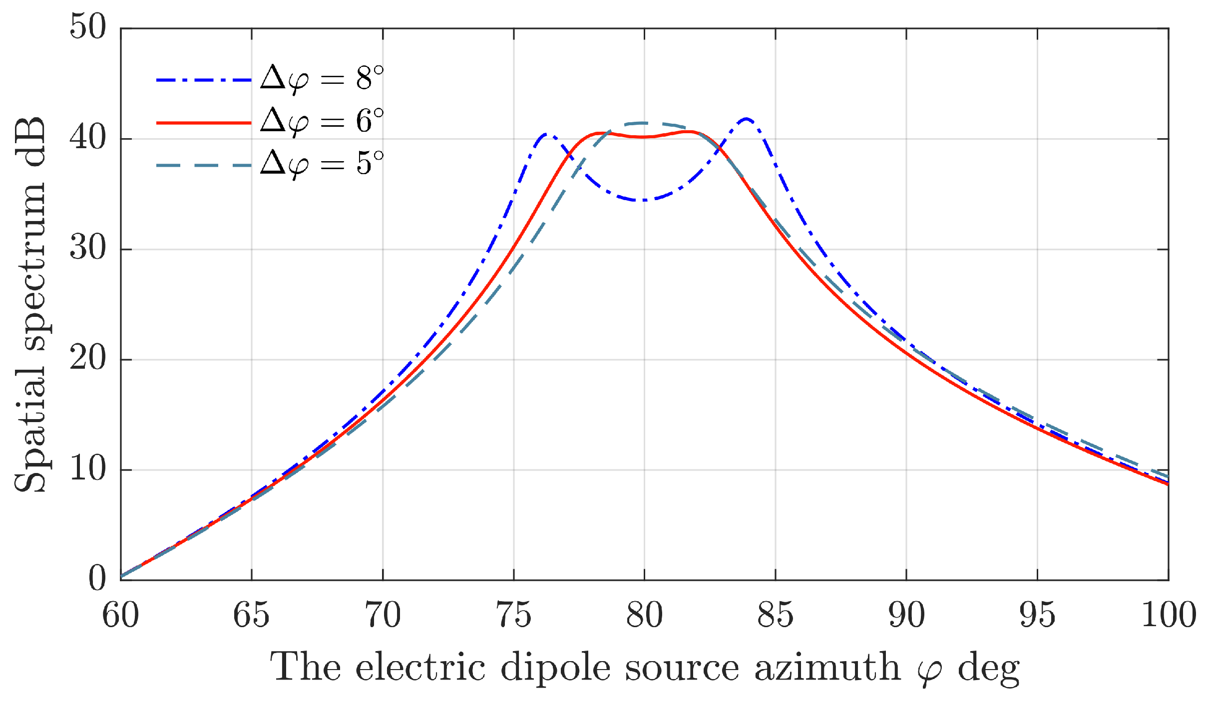
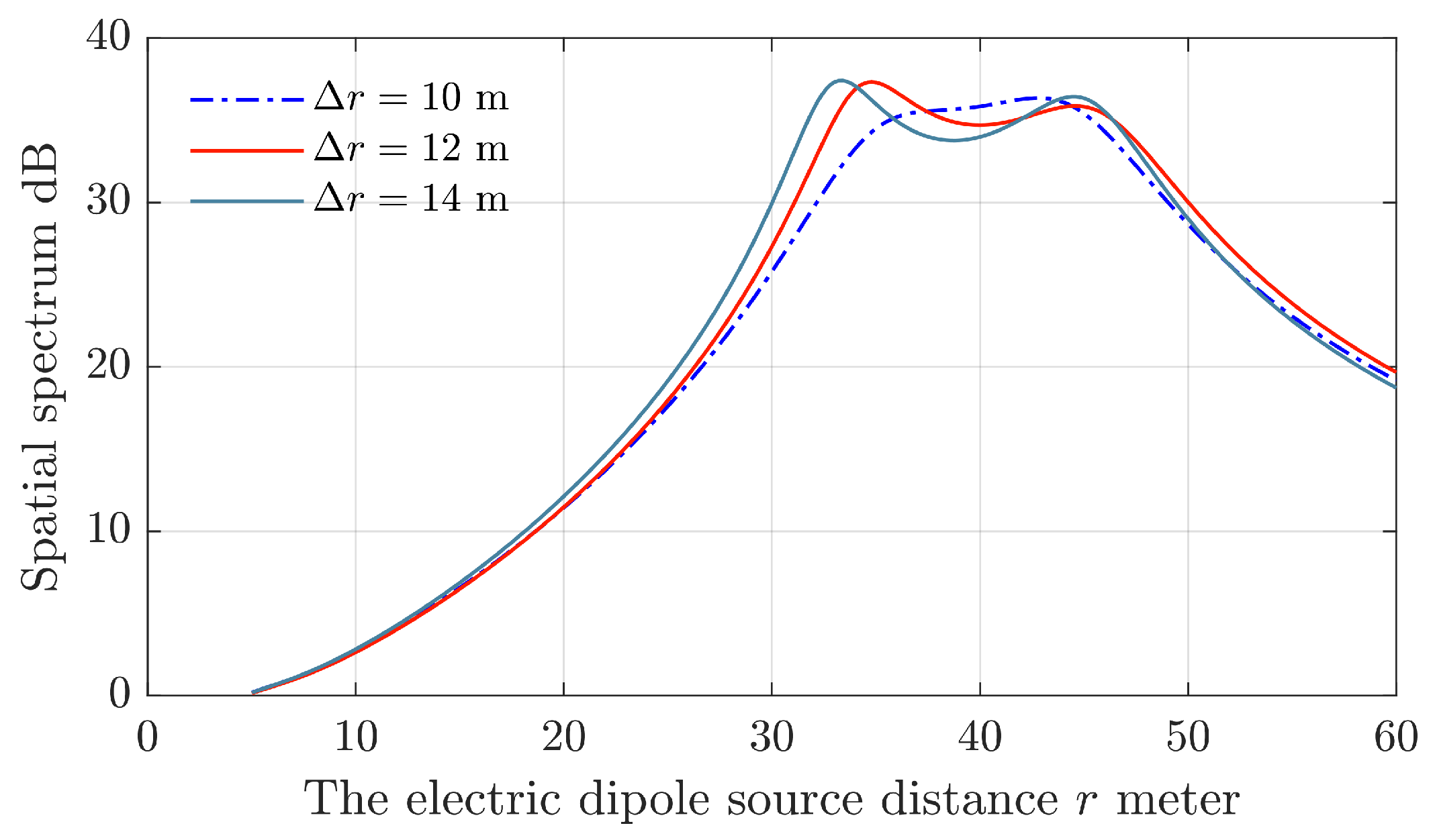
4.1. Resolution Analysis
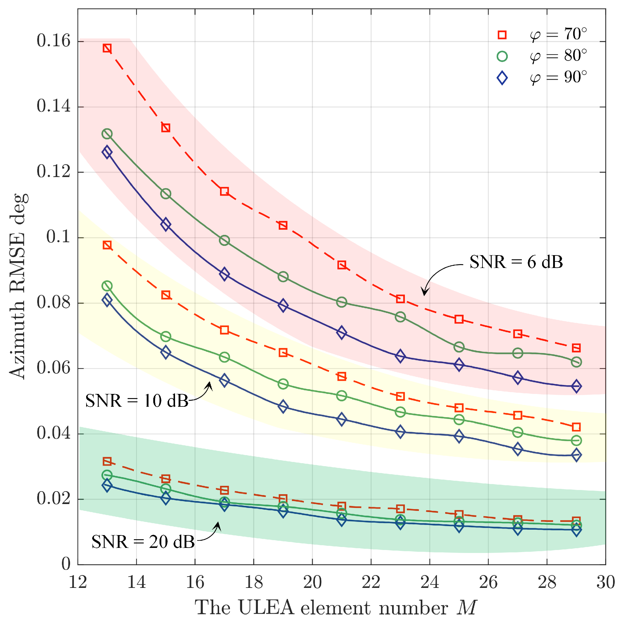
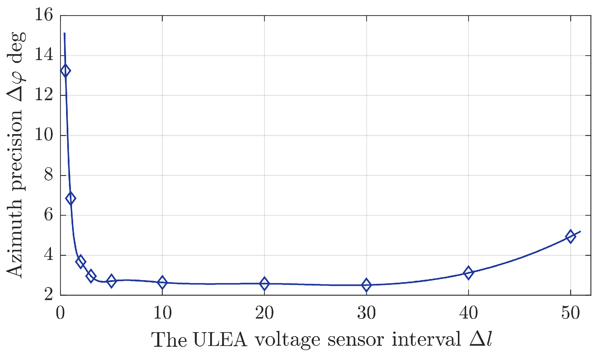
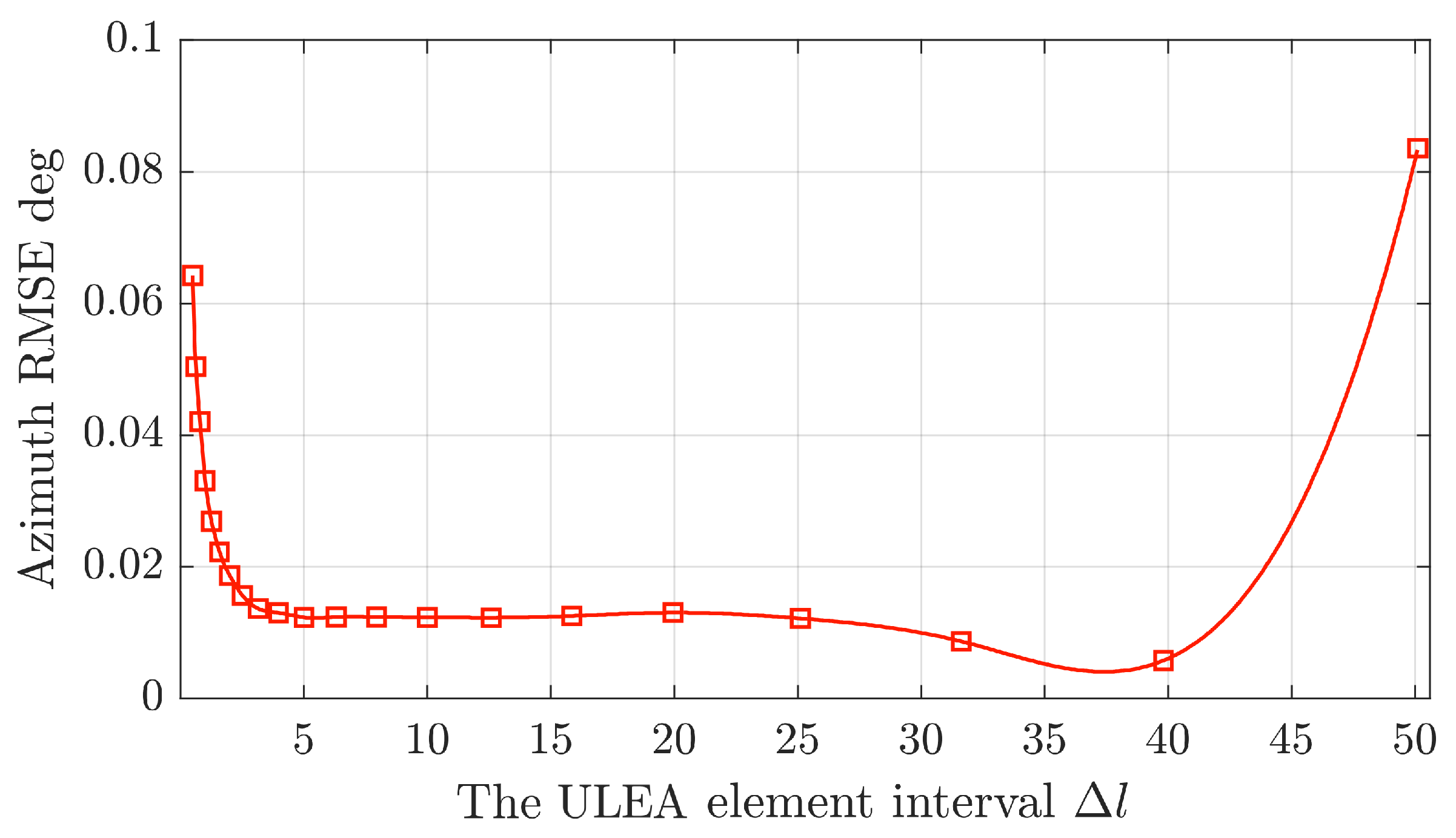
4.2. ULEA Structure & Locating Performance
5. Conclusions
Author Contributions
Funding
Institutional Review Board Statement
Informed Consent Statement
Data Availability Statement
Conflicts of Interest
References
- Park, D.; Kwak, K.; Kim, J.; Chung, W.K. Underwater sensor network using received signal strength of electromagnetic waves. In Proceedings of the 2015 IEEE/RSJ International Conference on Intelligent Robots and Systems (IROS), Hamburg, Germany, 28 September–2 October 2015; pp. 1052–1057. [Google Scholar]
- Quintana-Diaz, G.; Mena-Rodriguez, P.; Perez-Alvarez, I.; Jimenez, E.; Dorta-Naranjo, B.P.; Zazo, S.; Perez, M.; Quevedo, E.; Cardona, L.; Joaquin Hernandez, J. Underwater Electromagnetic Sensor Networks-Part I: Link Characterization. Sensors 2017, 17, 189. [Google Scholar] [CrossRef] [PubMed]
- Kim, J.H.; Jeon, J.C.; Yoo, J.G. The Measurement for the Underwater Electric Field Using a Underwater 3-Axis Electric Potential Sensor. In Proceedings of the International Conference on Grid and Distributed Computing, Jeju Island, Republic of Korea, 8–10 December 2011; pp. 408–414. [Google Scholar]
- Zhenbin, Z.; Bin, L. Underwater Electromagnetic Sources 2-D DOA and Polarization Estimation. In Proceedings of the 2012 Second International Conference on Industry, Information System and Material Engineering (IISME 2012), Wuhan, China, 17–18 March 2012; pp. 529–534. [Google Scholar]
- Boyer, F.; Lebastard, V.; Ferrer, S.B.; Geffard, F. Underwater pre-touch based on artificial electric sense. Int. J. Robot. Res. 2020, 39, 729–752. [Google Scholar] [CrossRef]
- Boyer, F.; Lebastard, V.; Chevallereau, C.; Mintchev, S.; Stefanini, C. Underwater navigation based on passive electric sense: New perspectives for underwater docking. Int. J. Robot. Res. 2015, 34, 1228–1250. [Google Scholar] [CrossRef]
- Zheng, J.; Wang, J.; Guo, X.; Huntrakul, C.; Wang, C.; Xie, G. Biomimetic Electric Sense-Based Localization: A Solution for Small Underwater Robots in a Large-Scale Environment. IEEE Robot. Autom. Mag. 2022, 29, 50–65. [Google Scholar] [CrossRef]
- Zhao, Z.; Hu, Q.; Feng, H.; Feng, X.; Su, W. A Cooperative Hunting Method for Multi-AUV Swarm in Underwater Weak Information Environment with Obstacles. J. Mar. Sci. Eng. 2022, 10, 1266. [Google Scholar] [CrossRef]
- Nguyen, N.; Wiegand, I.; Jones, D.L. Sparse Beamforming for Active Underwater Electrolocation. In Proceedings of the 2009 IEEE International Conference on Acoustics, Speech, and Signal Processing (ICASSP), Taipei, Taiwan, 19–24 April 2009; Volumes 1–8, pp. 2033–2036. [Google Scholar]
- Lim, H.S.; Ng, B.P.; Reddy, V.V. Generalized MUSIC-Like Array Processing for Underwater Environments. IEEE J. Ocean. Eng. 2017, 42, 124–134. [Google Scholar] [CrossRef]
- Lanneau, S.; Boyer, F.; Lebastard, V.; Bazeille, S. Model based estimation of ellipsoidal object using artificial electric sense. Int. J. Robot. Res. 2017, 36, 1022–1041. [Google Scholar] [CrossRef]
- Shang, W.; Xue, W.; Li, Y.; Wu, X.; Xu, Y. An Improved Underwater Electric Field-Based Target Localization Combining Subspace Scanning Algorithm And Meta-EP PSO Algorithm. J. Mar. Sci. Eng. 2020, 8, 232. [Google Scholar] [CrossRef]
- Yang, M.; Ding, J.; Chen, B.; Yuan, X. A Multiscale Sparse Array of Spatially Spread Electromagnetic-Vector-Sensors for Direction Finding and Polarization Estimation. IEEE Access 2018, 6, 9807–9818. [Google Scholar] [CrossRef]
- Schmidt, S.O.; John, F.; Hellbrueck, H. Evaluation of 3-dimensional Electrical Impedance Tomography-Arrays for Underwater Object Detection. In Proceedings of the OCEANS 2022, Chennai, India, 21–24 February 2022. [Google Scholar]
- Kim, J.; Son-Cheol, Y.; Bae, K.W. Calibrating Electrode Misplacement in Underwater Electric Field Sensor Arrays for the Electric Field-Based Localization of Underwater Vessels. J. Sens. Sci. Technol. 2022, 31, 330–336. [Google Scholar] [CrossRef]
- Wang, C.; Xu, Y.; Qi, J.; Shang, W.; Liu, M.; Chen, W. Passive Electromagnetic Field Positioning Method Based on BP Neural Network in Underwater 3-D Space. In Proceedings of the 5th EAI International Conference of Advanced Hybrid Information Processing (ADHIP 2021), Virtual Event, 22–24 October 2021; pp. 292–304. [Google Scholar]
- Liu, Z.; Gao, J.; Xu, L.; Jia, P.; Pan, D.; Xue, W. Electromagnetic Fusion Underwater Positioning Technology Based on ElasticNet Regression Method. In Proceedings of the 2022 IEEE 10th International Conference on Information, Communication and Networks (ICICN 2022), Zhangye, China, 23–24 August 2022; pp. 121–126. [Google Scholar]
- Peng, J.; Wu, J. A Numerical Simulation Model of the Induce Polarization: Ideal Electric Field Coupling System for Underwater Active Electrolocation Method. IEEE Trans. Appl. Supercond. 2016, 26, 0606305. [Google Scholar] [CrossRef]
- Peng, J.; Zhu, Y.; Yong, T. Research on Location Characteristics and Algorithms based on Frequency Domain for a 2D Underwater Active Electrolocation Positioning System. J. Bionic Eng. 2017, 14, 759–769. [Google Scholar] [CrossRef]
- Ren, Q.; Peng, J.; Chen, H. Amplitude information-frequency characteristics for multi-frequency excitation of underwater active electrolocation systems. Bioinspiration Biomim. 2020, 15, 016004. [Google Scholar] [CrossRef] [PubMed]
- Han, Y.; Wu, H.; Peng, J.; Ou, B. The Effect of Object Geometric Features on Frequency Inflection Point of Underwater Active Electrolocation System. J. Mar. Sci. Eng. 2021, 9, 756. [Google Scholar] [CrossRef]
- Liu, Y.; Hu, Q.; Yang, Q.; Li, Y.; Fu, T. An underwater moving dipole tracking method of artificial lateral line based on intelligent optimization and recursive filter. Meas. Sci. Technol. 2022, 33, 075113. [Google Scholar] [CrossRef]
- Peng, H.; Jiang, G.; Hu, Q.; Fu, T.; Xu, D. Locating and tracking of underwater sphere target based on active electrosense. Sens. Actuators Phys. 2023, 363, 114671. [Google Scholar] [CrossRef]
- Li, S.; Hu, Q.; Yang, Q.; Fu, T. Tracking the Underwater Moving Dipole with the Artificial Lateral Line Based on the PAST and KF. In Proceedings of the 2022 International Conference on Autonomous Unmanned Systems, ICAUS 2022, Xi’an, China, 23–25 September 2022; Lecture Notes in Electrical Engineering. Volume 1010, pp. 223–232. [Google Scholar]
- Wang, X.; Wang, S.; Hu, Y.; Tong, Y. Mixed electric field of multi-shaft ship based on oxygen mass transfer process under turbulent conditions. Electronics 2022, 11, 3684. [Google Scholar] [CrossRef]
- Kraichman, M.B. Handbook of Electromagnetic Propagation in Conducting Media; Headquarters Naval Material Command: Mechanicsburg, PA, USA, 1976. [Google Scholar]
- Friedlander, B.; Weiss, A.J. The resolution threshold of a direction-finding algorithm for diversely polarized arrays. IEEE Trans. Signal Process. 1994, 42, 1719–1727. [Google Scholar] [CrossRef]


| Azimuth | @ SNR = 6 dB | @ SNR = 10 dB | @ SNR = 20 dB |
|---|---|---|---|
| Distance r (Unit: m) | Resolution (Unit: m) |
|---|---|
| 10 | |
| 15 | |
| 20 | |
| 25 | |
| 30 | |
| 35 | |
| 40 | |
| 45 |
Disclaimer/Publisher’s Note: The statements, opinions and data contained in all publications are solely those of the individual author(s) and contributor(s) and not of MDPI and/or the editor(s). MDPI and/or the editor(s) disclaim responsibility for any injury to people or property resulting from any ideas, methods, instructions or products referred to in the content. |
© 2025 by the authors. Licensee MDPI, Basel, Switzerland. This article is an open access article distributed under the terms and conditions of the Creative Commons Attribution (CC BY) license (https://creativecommons.org/licenses/by/4.0/).
Share and Cite
Shang, W.; Gao, F.; Liu, J.; Pang, Y.; Volvenko, S.V.; Olshanskiy, V.M.; Xu, Y. Underwater Target Localization Method Based on Uniform Linear Electrode Array. J. Mar. Sci. Eng. 2025, 13, 306. https://doi.org/10.3390/jmse13020306
Shang W, Gao F, Liu J, Pang Y, Volvenko SV, Olshanskiy VM, Xu Y. Underwater Target Localization Method Based on Uniform Linear Electrode Array. Journal of Marine Science and Engineering. 2025; 13(2):306. https://doi.org/10.3390/jmse13020306
Chicago/Turabian StyleShang, Wenjing, Feixiang Gao, Jiahui Liu, Yunhe Pang, Sergey V. Volvenko, Vladimir M. Olshanskiy, and Yidong Xu. 2025. "Underwater Target Localization Method Based on Uniform Linear Electrode Array" Journal of Marine Science and Engineering 13, no. 2: 306. https://doi.org/10.3390/jmse13020306
APA StyleShang, W., Gao, F., Liu, J., Pang, Y., Volvenko, S. V., Olshanskiy, V. M., & Xu, Y. (2025). Underwater Target Localization Method Based on Uniform Linear Electrode Array. Journal of Marine Science and Engineering, 13(2), 306. https://doi.org/10.3390/jmse13020306