Enhanced AUV Autonomy Through Fused Energy-Optimized Path Planning and Deep Reinforcement Learning for Integrated Navigation and Dynamic Obstacle Detection

Abstract

Autonomous Underwater Vehicles (AUVs) operating in dynamic, constrained underwater environments demand sophisticated navigation and detection fusion capabilities that traditional methods often fail to provide. This paper introduces a novel hybrid framework that synergistically fuses a Multithreaded Energy-Optimized Batch Informed Trees (MEO-BIT*) algorithm with Deep Q-Networks (DQN) to achieve robust AUV autonomy. The MEO-BIT* component delivers efficient global path planning through (1) a multithreaded batch sampling mechanism for rapid state-space exploration, (2) heuristic-driven search accelerated by KD-tree spatial indexing for optimized path discovery, and (3) an energy-aware cost function balancing path length and steering effort for enhanced endurance. Critically, the DQN component facilitates dynamic obstacle detection and adaptive local navigation, enabling the AUV to adjust its trajectory intelligently in real time. This integrated approach leverages the strengths of both algorithms. The global path intelligence of MEO-BIT* is dynamically informed and refined by the DQN’s learned perception. This allows the DQN to make effective decisions to avoid moving obstacles. Experimental validation in a simulated Achao waterway (Chile) demonstrates the MEO-BIT* + DQN system’s superiority, achieving a 46% reduction in collision rates (directly reflecting improved detection and avoidance fusion), a 15.7% improvement in path smoothness, and a 78.9% faster execution time compared to conventional RRT* and BIT* methods. This work presents a robust solution that effectively fuses two key components: the computational efficiency of MEO-BIT* and the adaptive capabilities of DQN. This fusion significantly advances the integration of navigation with dynamic obstacle detection. Ultimately, it enhances AUV operational performance and autonomy in complex maritime scenarios.

1. Introduction

With the increasing application of intelligent marine vehicles, especially autonomous underwater vehicles (AUVs), efficient autonomous navigation systems are required in environmental monitoring, cargo transportation, coastal surveillance, inland waterway navigation, port operations, and autonomous ferry services [1,2]. As the key problem of autonomous navigation, path planning directly impacts the safety, efficiency, and endurance of AUVs (including Unmanned Surface Vehicles (USVs)) operating in narrow waterways [2]. However, despite their robustness, common search-based planners, such as the classic A* algorithm and its variations, are often inefficient in narrow waterways or for surface navigation. Sampling-based planners such as Rapidly-exploring Random Tree Star (RRT*), Batch Informed Trees (BIT*) [3] can find feasible paths efficiently in high-dimensional space but often provide suboptimal or unstable trajectory information, which increases cost and results in poor maneuvering efficiency; furthermore, they cannot guarantee good stability and robustness in complicated environments with unpredictable obstacles, requiring frequent replanning, which is very inefficient. BIT* works well in static and quasi-static environments, but it is not easy to apply in dynamic obstacle fields. It lacks the adaptability and intelligence to make active and wise decisions. On the contrary, pure Deep Reinforcement Learning (DRL) methods such as Deep Q-Networks (DQN) perform poorly in sample efficiency and will take a long time to learn in an uncertain environment. DQN-based policies show potential for adapting to complex maritime environments. However, their real-world application can be impractical or unsafe. This is because they require extensive converging interactions, making them unsuitable for most maritime operations [4]. Therefore, it is necessary to combine sampling-based geometric planners with DRL agents to obtain more effective, robust, and brilliant solutions for navigation under various complex conditions. Therefore, we identify the need for new path planning approaches by summarizing existing literature in this paper. Navigating in a narrow waterway requires not only path feasibility and distance optimality but also other essential aspects that should be considered, such as collision avoidance (paramount factor), minimizing travel time, smooth turning motion (operational efficiency), and conserving energy (cost). This results in limited options for IMVs, such as AUVs, in dynamic/narrow waterways. Traditional solution paradigms either lack robustness and efficiency in practical scenarios or do not offer safe, reliable, and knowledgeable guidance.

To address the above issues and challenges, a multithreaded energy-optimized BIT* + DQN hybrid path planner is proposed in this paper to make full use of the complementary advantages of BIT* with multiple threads running simultaneously and DQN, which provides local optimization strategies while effectively learning how to predict, avoid dynamic obstacles, and optimize several objectives, including, but not limited to, energy consumed. The research question being addressed in this paper is: “Can a synergistic combination of both worlds enable IMVs to gain better robustness, efficiency, and intelligence for successful operation and achieve true autonomy?” By combining the exploration ability of sampling-based geometry path planner BIT* and the exploitation capability of DRL, a Multithreaded Energy Optimized BIT* + DQN path planner algorithm was developed. Our contributions in this work are as follows:

A novel hybrid path planning framework (MEO-BIT* + DQN) is proposed. This framework synergistically integrates the efficient global path generation and heuristic guidance capabilities of an advanced sampling-based geometric planner, Multithreaded Energy-Optimized Batch Informed Trees (MEO-BIT*), with the robust capabilities of a Deep Q-Network (DQN) for adaptive local path optimization and dynamic obstacle avoidance in complex narrow waterways, thereby overcoming the limitations of standalone geometric or learning-based approaches.

A significantly enhanced MEO-BIT* algorithm is presented, achieving efficient and energy-aware global planning through the introduction of three core innovations: (a) a multithreaded batch sampling mechanism incorporating heterogeneous CPU core management to reduce planning time significantly; (b) an optimized heuristic search integrated with k-dimensional tree (KD-tree) acceleration to improve nearest-neighbor search efficiency; and (c) the construction and integration of a physics-inspired cost model to generate near-optimal paths that balance both distance and actual cost efficiency.

An effective DQN-guided local optimization and dynamic adaptation strategy was also developed. This strategy empowers the DQN agent to use the output of MEO-BIT* for state representation, learn intelligent obstacle avoidance maneuvers, and potentially guide the MEO-BIT* search process. This significantly boosts the system’s robustness in dynamic environments and enhances global–local planning efficiency.

Comprehensive experimental validation was conducted. Simulation results in real-world complex and narrow waterway environments with dynamic obstacles, such as the Achao waterway in Chile, demonstrate that the proposed MEO-BIT* + DQN method significantly outperforms baseline algorithms in terms of reduced collision rates, improved path smoothness, optimized cost efficiency, and enhanced computational speed. This provides strong experimental support for the autonomous navigation of intelligent marine vehicles.

1.1. BIT* Algorithm and Its Research Status and Challenges in Energy and Dynamic Adaptability

The BIT* algorithm incrementally constructs an implicit random geometric graph through a batch-processing approach. Then, dynamic programming searches for the optimal path within this graph. It exhibits significant computational advantages in high-dimensional, complex environments, capable of quickly finding feasible solutions and progressively optimizing them toward an optimal solution [3,5]. As an algorithm developed from sampling-based planning concepts such as RRT*, BIT* aims to improve initial suboptimal paths through heuristic global techniques and local optimization, achieving superior planning results and convergence toward a worldwide optimum [6]. Gammell et al. [5] have demonstrated BIT*’s probabilistic completeness, asymptotic optimality, and efficiency in high-dimensional spaces. Based on BIT*, researchers have proposed improvements: Choudhury et al.’s raBIT* [7] accelerates the search by incorporating a local optimizer (such as CHOMP), which is particularly effective in narrow passages. Zhang et al.’s fit* [8] optimizes BIT*’s efficiency across different dimensional spaces through an adaptive batch-sizing strategy. Cao et al.* [9] utilize error-tolerant points to increase path diversity and evade obstacles in dynamic environments. At the same time, Zheng and Tsiotras’s ibbt [10] extends BIT* to belief-space planning in uncertain environments. Research in related fields also offers insights for handling complex constraints and dynamic environments. For instance, RRT*-Smart [11] enhances RRT* efficiency through heuristic sampling and gradual optimization, sharing BIT*’s objective of efficient optimal path planning in high-dimensional, complex environments. Yang et al.’s SRRT [12] efficiently addresses robot differential constraints using spline curve parameterization, providing ideas for integrating complex kinematic constraints into sampling optimization algorithms. Li et al. [13] proposed the SST and SST* algorithms specifically for dynamic environments lacking precise BVP solvers. Their work demonstrates that even with limited system model information, asymptotically (near-)optimal path planning can be achieved with fast convergence. This provides a significant theoretical and practical reference for applying BIT*-like algorithms in complex dynamic scenarios, especially regarding achieving planning optimality with more restricted system model information. SRRT’s method of efficiently handling internal and external constraints while ensuring path curvature continuity via spline curves also offers valuable insights for sampling optimization algorithms, including BIT*, when dealing with specific motion constraints.

1.2. Current Research Status of Artificial Intelligence Deep Reinforcement Learning

Deep Reinforcement Learning (DRL), a cutting-edge technology in artificial intelligence, demonstrates immense potential in addressing autonomous decision-making problems within complex dynamic environments by combining the perceptual capabilities of deep learning with the decision-making abilities of reinforcement learning. It has garnered significant attention, particularly in the domain of robot navigation. Unlike traditional planning algorithms, DRL methods can acquire optimal strategies through interaction with the environment, allowing them to better adapt to uncertainty and dynamic changes.

In recent years, researchers have extensively explored the application of DRL to various navigation tasks. For example, Sivayazik and Mannaye [14] proposed a double DQN-based algorithm for autonomous vehicle navigation in urban dynamic obstacle environments, optimizing neural network structures and reward functions across different training settings. Deguale et al. [15] introduced an improved DRL strategy combining prioritized experience replay, reward shaping, and specific network architectures (such as PMR-Dueling DQN). They validated its effectiveness in robot path optimization, obstacle avoidance, and learning speed within grid worlds and Gazebo simulation environments. These studies indicate that DRL can guide agents to learn effective navigation behaviors through carefully designed reward mechanisms and network structures.

Meanwhile, remarkable achievements have been made in using DRL to solve special navigation situations. Zhang et al. [16] designed the Pro-Polishing DQN algorithm and solved the problems of slow convergence and experience waste in mobile robot local path planning using a sum tree-based priority experience replay method to improve learning efficiency and path quality; Yang et al. [17] improved the DQN algorithm by optimizing the sample collecting and non-uniform sampling strategies and applying them to intelligent anti-collision for vessels; Yang et al. [18] first constructed an environmental model based on an electronic chart and altitude map, then designed a DQN algorithm-based path planning scheme for amphibious uncrewed surface vehicles, and improved path rationality by action masking and path smoothing; Wen et al. [19], combining MonoDepth with obstacle recognition, proposed a probabilistic dueling DQN algorithm to optimize agent paths, which could make the agent converge faster. It was mixed with FastSLAM to realize autonomous navigation and mapping. For coastal ship path planning, Guo et al. [20] introduced an optimized DQN path planning model, quantified the real-world navigation environment and collision avoidance rules to guide DQN’s learning, and improved the path safety and economy levels. Yang et al. [21], and then Noreen et al. [22], used the DQN algorithm to combine Q-learning, experience replay, and other network structures, such as physics output neural networks, to solve multi-robot path planning problems. Yuan et al. [23] focused on cross-river path planning of inland ferries, designed and improved the state space, action space, and reward function of the DQN model, and completed economical and safe autonomous ferry navigation. Lv et al. [24] put forward improved learning methods according to different learning needs, among which the Q-value calculation of DQN was based on a dense network frame structure, accelerating the convergence speed and improving path accuracy. Li et al. [25] introduced a new DRL-based unified collision avoidance path planning strategy, and simulation tests verified its effect under different conditions. Huang et al. [26] presented an improved DQN algorithm for the path planning of uncrewed surface vehicles (USV). Further, Villanueva et al. [27] combined Double Q-learning with a Dueling architecture to achieve effective UAV path planning, while Zhou et al. [28] further studied DRL in USV single-vessel/formation path planning, exceptionally reliable collision avoidance in restricted seas.

Although the excellent potentials shown in the above DRL literature have indicated that there is a tendency to use them on navigational applications, as well as with improvement from various advanced technical usages such as the prioritized experience replay method, reward shaping technique, specific network structure setting up, and combination of other algorithm approaches, pure reinforcement learning techniques are still facing many problems at present. Sample inefficiency is also unavoidable here; agents must interact longer and make mistakes before they exhibit efficient behavior; meanwhile, this cost would be even more expensive and risky for reasons concerning the reality of the maritime domain [29]. Meanwhile, stability of convergence and lack of sub-optimal solutions may need careful design, especially when there is a lack of sufficient prior knowledge guidance support for avoiding such situations accordingly [30]. Moreover, how the existing geometric planner benefits from the structure of DRL and guides or instructs itself about the path learning process, i.e., how to combine that specific knowledge/answers, seems another direction worth exploring. How to realize it remains unknown.

Therefore, taking into consideration all that has been stated above about the nature of reinforcement learning algorithms’ characteristics—i.e., its unique feature of being good enough with decision-making in dynamics but bad for adaptation—and that its potential might further increase by using an adequate sampling search approach rather than exhaustive random searching (e.g., by using our improved MEO-BIT* planner efficiently)—we believed that hybridizing our designed planning architecture with a deep learning reinforcement technique would achieve good and satisfactory results, including increasing adaptability and collision-free levels.

2. MEO-BIT* + DQN Hybrid Path Planning Framework

To realize an intelligent ship’s safe, effective, strong, and energy-saving autonomous navigation in complex and narrow waterway channels, this paper puts forward a hybrid planning structure combining MEO-BIT* and Deep Q-Networks (DQN) to organically incorporate their advantages, fully consolidate the powerful global efficient path producing method MEO-BIT*’s ability, and complete the consolidation of the local intelligent decision algorithm based on dynamic environment adaptation provided by the Q-learning mechanism DQN, avoiding one-sidedness.

2.1. High-Performance Multithreaded Energy-Optimized (MEO-BIT*) Model

2.1.1. Batch Sampling and Heuristic-Guided Mechanism

The core of the MEO-BIT* algorithm is the intelligent strategy combining the advantage of batch sampling with guided heuristics to search in complicated continuous-state spaces, which begins by first dividing the original continuous-state space into batch-sampled random sample points, using an implied RGG for reference about their potential inter-relationships. The edge evaluation of BIT* does not have to be computed simultaneously; it evaluates edges using a heuristic at any time according to needs, saving tremendous amounts of edge evaluation calculation operations, especially when facing large search volumes.

To conduct effective searching processes, the key point is keeping two different priority queues updated—vertices’ and edges’ priority queues, respectively named QV and QE—with the vertices’ waiting queue, QV, containing all those awaiting to be processed, stored, and sorted based on the estimation between these vertexes from the start to the goal, including distance and cost together; this sorting method is named the Total Cost Ordering TC Order (TCo). The edges’ waiting queue (QE) contains all of those edges under evaluations stored in sorted order, TCOrder (which sorts both distance AND energy costs), from the start to the goal, referred to by us as EEdges TCO (EE-TCo). Thus, 2-PQ management combined with MEO-BIT*(search process) gives us a higher likelihood of chance paths (that hopefully converge better solutions than prior ones encountered up until now while expanding BTTree*) during its iterative procedures whenever available.

The evaluation function is given by Equation (1):

$$f\left(v\right)=g_T\left(v\right)+\widehat{h}\left(v\right),$$

(1)

where $g_T\left(v\right)$ represents the current known lowest cost (considering energy) from the start to vertex v, and $\widehat{h}\left(v\right)$ represents the estimated cost (considering energy) from vertex v to the target.

The batch sampling process of MEO-BIT* optimizes the batch strategy, and the algorithm can add a group of new samples (the number of which can be set freely) per iteration. After searching for the current batch, prune the unnecessary nodes, then add new batches according to the need to ensure convergence and improve the efficiency of path discovery.

The main innovation mechanisms in the batch sampling process of MEO-BIT* are threefold, designed to enhance both exploration efficiency and solution quality:

Just-In-Time (JIT) Sampling: Instead of pre-discretizing the entire search space, this mechanism allows the algorithm to dynamically generate sample points during the search process based on current needs. This makes MEO-BIT* highly flexible and particularly suitable for navigating vast or unstructured open waters, as it dynamically determines the amount of information needed at the frontier. The number of required samples is calculated using Formula (2):

$$c_{req}^0\left(d\right)=\mathit{min}\left(c_i,\underset{x\in X_{near}}{\mathit{max}}\widehat{f}\left(x\right)\right).$$

(2)

Optimized Sampling Strategy: MEO-BIT* synergistically combines both direct and random sampling. The probability of using direct sampling is adaptively controlled by heuristic evaluations, prioritizing regions with a high likelihood of containing the optimal solution. This accelerates the generation of high-quality samples while maintaining diversity. After finding an initial feasible solution, the strategy focuses on refining the current path while preserving global exploration. Optimized Sampling Strategy: MEO-BIT* synergistically combines both direct and random sampling. The probability of using direct sampling is adaptively controlled by heuristic evaluations, prioritizing regions with a high likelihood of containing the optimal solution. This accelerates the generation of high-quality samples while maintaining diversity. After finding an initial feasible solution, the strategy focuses on refining the current path while preserving global exploration.

Adaptive Batch Size Mechanism: This mechanism intelligently regulates the number of samples processed in each iteration. In the initial search phase (when no solution exists), increase the batch size to accelerate exploration and cover the space efficiently. Once a feasible solution is found, it progressively reduces the batch size, allocating more computational resources for path refinement. This creates a dynamic balance between exploration and optimization, which is especially advantageous in environments where fixed sampling strategies underperform.

Explicitly speaking, at the beginning of the algorithm, without any valid solution, this adaptive batch-size adjustment strategy will force the value up, enabling the batch process to search more efficiently. However, after getting the desired solution initially found successfully, another adjustment factor proportional to the former one will be used to decrease the batch size, allowing more time for refinement along the already chosen route and making the search balance between exploration and optimization finely adjusted dynamically according to their requirements in different situations. This approach is advantageous in vast or unstructured open-water environments where fixed sampling strategies underperform.

MEO-BIT* synergistically combines direct and random sampling strategies. The direct sampling probability parameter is adaptively controlled based on heuristic evaluations indicating high-probability optimal solution regions. This optimization accelerates high-quality sample generation during iterations while maintaining solution diversity. After obtaining an initial feasible solution, the strategy focuses on the current solution while preserving global exploration capability to ensure asymptotic optimality.

This component intelligently regulates sample volume per iteration cycle. During initial search phases (no valid solution), the mechanism prioritizes exploration by increasing the batch size for efficient space coverage. Upon obtaining a feasible solution, the batch size is progressively reduced using a decay factor proportional to solution quality. This creates a dynamic balance between:

Exploration: Broad search space coverage

Optimization: Local path refinement

The adaptive adjustment responds to changing search conditions in real time, optimizing resource allocation throughout the planning process.

2.1.2. Multithreaded Parallel Optimization Mechanism

The MEO-BIT* algorithm used in this study fully uses the computational advantages of modern heterogeneous processors. This type of processor, such as the Intel Core i7-14700H used in this experiment, typically contains two different types of cores:

Performance Cores (P-Cores): Designed to handle high-load and compute-intensive tasks. With higher clock frequencies and stronger single-core performance, they are suitable for performing latency-sensitive critical calculations in algorithms, such as complex collision detection or path evaluation.

Efficiency Cores (E-Cores): Designed for background tasks, I/O operations, and highly parallel, multithreaded loads. They are more advantageous regarding power consumption and are suitable for performing non-core but continuously running tasks such as monitoring, data management, etc.

By implementing intelligent thread scheduling and load balancing on this hybrid architecture, our algorithm can allocate different types of computing tasks to the most suitable core execution, thereby optimizing overall energy efficiency while maximizing computing throughput. The following is a detailed description of the specific parallel optimization mechanism we designed for this architecture.

Different heterogeneous thread pools management: For different demands of the computation task (colliding, dense sample, etc.), it will assign special threads so that other threads and pools will be assigned for I/O and less demanding loads, e.g., monitor run status, manage auxiliaries to E-cores (Efficiency cores, optimized for low-power background tasks) rather than heavy computation, as they cannot benefit from multiple parallel computation, and P-core (Performance cores) can make better improvement in single-thread application. However, other cases, such as input/output or search status monitoring, could also be done using available free-up E-cores. The balance number has to be put down by us, which shall be used for computations where all cores would have been engaged, but the perfect number of those threads relies upon the physical/core configuration that is represented by Equation (3):

$$N_{opt}=\mathit{min}\left(N_{\mathit{physical}\_\mathit{cores}}\times 1.5,{ N}_{\mathit{logical}\_\mathit{cores}}\right),$$

(3)

where $N_{\mathrm{physical}\_\mathrm{cores}}$ is the number of physical cores and $N_{\mathrm{logical}\_\mathrm{cores}}$ is the number of logical cores.

Dynamic Load Balancing: It dynamically changes the length and priority of the work item queues based on the load situation of each CPU core, ensuring that it is uniformly distributed between P-cores and E-cores. At the same time, it adopts the work-stealing strategy; when a core (especially an E-core or an idle P-core) finishes one task, it can steal tasks from other busy cores’ (especially P-core’s) tail-end work item lists to execute them simultaneously. This is very important in the case of large maps being processed or intense explorations occurring—otherwise, this could cause computational bottlenecks, which would restrict the maximum output of the whole system.

Batch Collision Detection Optimization: MEO-BIT* organizes collision detection tasks for multiple edges into batches rather than performing independent, sequential collision checks for each newly generated edge. These batched tasks, containing multiple edges, are then processed in parallel by multiple threads within a thread pool. This batch-processing method significantly reduces the overhead of single-task scheduling and thread synchronization, leading to substantial acceleration in complex environments with numerous potential path segments. Collision detection itself uses the Bresenham line algorithm for discretized checks, further optimized by a Bresenham algorithm caching mechanism: previously checked line segments and their collision status are cached to avoid redundant checks on identical or similar segments in subsequent iterations (especially during iterative path refinement). The collision detection resolution can be set as needed (e.g., 20 units), and the batch size for batch collision detection is also configurable (e.g., 200 edges).

Thread Affinity Optimization: MEO-BIT* employs a thread affinity optimization strategy to minimize context switching overhead caused by threads migrating between different CPU cores and improve CPU cache coherence and hit rates; MEO-BIT* employs a thread affinity optimization strategy. Threads responsible for critical, long-running tasks (e.g., managing updates to specific KD-tree branches or maintaining particular sections of priority queues) can be pinned to dedicated CPU cores (typically P-cores for compute-bound tasks or particular E-cores for consistent background tasks) for execution. This practice ensures that the relevant thread’s data remains as much as possible in the corresponding core’s local cache, reducing memory access latency.

KD-Tree Accelerated Nearest Neighbor Search: To increase the performance gain achieved by using KD-tree in the nearest neighbor search of sampled points (the sampling process consists mainly of nearest neighbor search operation), once again, adopt the advanced data structure named KD-Tree to find the closest vertex within the existing tree of sampled points (which usually contains lots of samples). As a result, compared with the naive case of acceleration function, where the environment scale expands too fast and the number of all searchable vertices increases dramatically, then adopting the above-accelerated KD-searching method would benefit the algorithm quite a lot.

Dynamic resolution change technology: MEO-BIT*, taking different path segment length accuracy requirements into account, uses higher-precision dynamic adjustment collision detection accuracy for shorter paths and lower-precision dynamic adjustment collision detection accuracy for longer paths by dynamically calculating the number of search points according to the following Formula:

$$N_{\mathit{divs}}=\mathit{max}\left(MIN SEGMENT CHECK,⌊scale\times dist⌋\right).$$

The entire multithreaded parallel optimization mechanism is illustrated in Figure 1.

2.1.3. Cost Equation Optimization Mechanism

The cost equation optimizing mechanism is another innovative feature between the MEO-BIT* algorithm and the traditional path planners. The traditional ones only optimize the paths in consideration of geometrical length without considering most of the whole cost resulting from the ship’s turning behaviors (such as the number of maneuvers and value of maneuvers) etc., on which we put forward a general comprehensive cost function-balancing path length ($d$) and turning penalty ($\theta$), defined as, which is the ideal index for the intelligent ocean-going vehicle to seek total navigation consumption compared with the actual situation when planning voyages.

The fundamental form of this cost function is defined as:

$$E=\alpha ·d+\beta ·\theta ·\omega .$$

(4)

This cost function incorporates insights from hydrodynamics, where the turning term $\left(\beta · \theta · \omega \right)$ penalizes maneuvers that typically increase the actual cost (e.g., due to increased drag during turns), and θ means the turning angle that appears when sailing. This value comes from the calculation result of the angle between the current path segment and the previous path segment (or the angle between two adjacent path segments), which is expressed explicitly in Equation (5):

$$\theta =\arccos \left(\frac{\overrightarrow{v_1}·\overrightarrow{v_2}}{\left|\overrightarrow{v_1}\right|\left|\overrightarrow{v_2}\right|}\right)·\frac{180}{\pi }.$$

(5)

Degree-to-radian conversion is where Equation (5) correctly expresses the local curvature value of the path. α means the distance weight factor; its role is to adjust the basic ship energy expenditure required to overcome factors such as hydrodynamic drag and the ship’s energy consumed per unit distance while sailing. β is the steering weight factor; its role is to add an extra energy penalty for the sudden or large-angle steering appearing in the sailing process. Severe turning will not only cause an increase in cost, due to overcoming resistance generated by the rudder and hull sideways moving laterally in the water, but may also have adverse effects on navigation stability and board equipment or items’ safety. Adjusting the ratio relationship between α and β, for example, if β > α, means we can drive the MEO-BIT* algorithm to focus more attention on evaluating whether the generated path passes through areas with high energy losses caused by sudden turns. ω means the correction coefficient of the turning angle; here, for calculation convenience, it is preliminarily considered that a linear correspondence relationship exists between the turning angle and obtained extra energy cost (i.e., ω = const.), for example, taking 1.0. Of course, the setting of this parameter leaves us enough room to carry out in-depth research further to introduce some nonlinear models to better evaluate the specific influence of different sizes and angular velocities of turns on ship costs.

Of course, regarding these key parameters, their reasonable values must be calibrated based on preliminary sensitivity analysis according to the special application situation (such as ship type and water environment) before they are used. The purpose is to seek the optimal balance between the shortest path length and maximum action smoothness (the minimum energy). Only such carefully tuned energy-aware path evaluation mode can provide more effective realistic reference hint information for the searching process itself of the MEO-BIT* algorithm; at the same time, it can provide richer and more informative energy-estimating baseline hint information for any integrated DQN module after formation in the subsequent policy learning stage, in order to drive DQN to learn how to sail in a more energy-saving way gradually.

The energy cost E (Equation (4)) effectively integrates into the MEO-BIT* algorithm’s path evaluation. This directly governs the edge evaluation function f(edge) and indirectly refines h(v)’s search estimate for future paths. Consequently, the MEO-BIT* planner’s expansion decisions prioritize not merely geometric shortest paths but energy-optimized, geometrically suitable paths.

Crucially, these optimal path candidates must offer both broader scope minimality and, more critically, globally lower costs, considering overall expected travel costs and efficiency. Local path choices during global searches often incur excessive energy and time if viewed as final routes. This is vital for long-endurance AUV missions (e.g., exploration or surveying), as energy-oriented global planning provides ample operational time, maximizing range and mission duration under reasonable conditions. Figure 2 visually demonstrates how energy optimization influences planned routes, contrasting unoptimized paths with energy-optimized alternatives to validate global optimality. Other control mechanisms refine trajectories to meet mission requirements while reducing total cost.

2.2. Theoretical Deepening, Parameter Optimization Considerations, and Impact Mechanism of the Cost Equation

To ensure the MEO-BIT* algorithm effectively balances distance cost and turning cost during path evaluation, the weight parameters in the cost equation (see Equation (4)) were meticulously set. In this study, the distance weight α is set to 1.0, serving as the basic cost measure. The turning weight β is set to 1.25 to impose a moderate penalty for drastic turns during navigation, guiding the algorithm to generate smoother, lower-energy paths. The turning angle correction coefficient ω is set to 1.0, assuming a linear relationship between the turning cost and angle for model simplification. These parameter values were determined through a preliminary sensitivity analysis—testing different α/β combinations on representative waterway segments and observing path shape, estimated total cost, and obstacle avoidance success rate—based on understanding each parameter’s physical meaning. The aim was to prioritize successful obstacle avoidance while considering path length and cost efficiency. This specific parameter combination (α = 1.0, β = 1.25, ω = 1.0) is designed to provide a reasonable, efficient, and informative initial energy evaluation benchmark for the subsequently integrated Deep Reinforcement Learning (DQN) module, thereby assisting DQN in learning more optimal navigation strategies. Figure 3 illustrates the overall flow of the MEO-BIT* algorithm, which incorporates this energy optimization mechanism.

2.3. MEO-BIT* + DQN Hybrid Path Planning Strategy Model

This study proposes a novel hybrid path planning strategy suitable for complex inland river environments. This strategy deeply integrates the high efficiency of the MEO-BIT* model in global path search and energy optimization with the powerful capabilities of the Deep Q-Network (DQN) algorithm in handling dynamic environments and learning complex decision-making behaviors. This hybrid strategy aims to provide high-quality initial paths and heuristic information through synergistic action. At the same time, DQN performs local, real-time path adjustments and dynamic obstacle avoidance. This significantly enhances the autonomous navigation efficiency and robustness of intelligent marine vehicles in complex dynamic environments, all while ensuring navigation safety and path economy. To achieve this, the model’s design incorporates efficient mathematical modeling methods. It optimizes DQN’s learning and planning performance in dynamic environments through specific reward mechanisms and network structures, ensuring the practicality of the final generated navigation solutions.

The successful training and performance of the MEO-BIT* + DQN hybrid model critically depend on the reasonable setting of a series of initialization parameters, among which the neural network weight initialization and experience replay buffer-related parameters of the DQN module are critical.

Initial weight states significantly impact training for the DQN model’s Q-Network and Target Q-Network. This study uses a standard normal distribution random initialization (mean 0, standard deviation 0.01) to break symmetry, prevent local optima, and promote effective learning. While employed here, more advanced methods, such as Xavier or He initialization, could be explored in future work to maintain activation value means and variances better across layers, mitigating vanishing/exploding gradients, and accelerating convergence.

2.3.1. Extended Reading

To assist DQN knowledge learning successfully and eliminate early-stage training sample vanishing and exploding gradient issues (in the online network as well as the Q-network plus target network), this chapter corresponds to all kinds of initialization layer weights. The random initialization method used is selected from Xavier, and using these parameters at the start setting makes sample training possess a proper level of shared activity value out.

2.3.2. Experience Replay Buffer Settings

Methods such as Xavier and He are used to initialize weights cleverly so that the gradients do not vanish or explode—they ensure that the output variance is consistent across layers. This improves efficiency and ensures stability during training. The correct initialization method depends on the problem so that it converges quickly.

(1)

Other Hyperparameter Settings

The practical training of the DQN module relies on carefully selected hyperparameters. In this study, the key hyperparameters were set as follows, with specific values detailed in

Table 1. Hyperparameter settings for training the DQN decision model.

Hyperparameter Name	Value
Maximum Steps	100
Replay Buffer Size	20,000
Initial Exploration Rate ${\epsilon }_{initial}$	0.9
$\mathrm{E}\mathrm{x}\mathrm{p}\mathrm{l}\mathrm{o}\mathrm{r}\mathrm{a}\mathrm{t}\mathrm{i}\mathrm{o}\mathrm{n} \mathrm{D}\mathrm{e}\mathrm{c}\mathrm{a}\mathrm{y} \mathrm{R}\mathrm{a}\mathrm{t}\mathrm{e} {\epsilon }_{decay}$	0.995
$\mathrm{F}\mathrm{i}\mathrm{n}\mathrm{a}\mathrm{l} \mathrm{E}\mathrm{x}\mathrm{p}\mathrm{l}\mathrm{o}\mathrm{r}\mathrm{a}\mathrm{t}\mathrm{i}\mathrm{o}\mathrm{n} \mathrm{R}\mathrm{a}\mathrm{t}\mathrm{e} {\epsilon }_{min}$	0.1
$\mathrm{D}\mathrm{i}\mathrm{s}\mathrm{c}\mathrm{o}\mathrm{u}\mathrm{n}\mathrm{t} \mathrm{F}\mathrm{a}\mathrm{c}\mathrm{t}\mathrm{o}\mathrm{r} \gamma$	0.9
Learning Rate	0.001
Batch Size	32
Update Frequency	200

:

Discount Factor (γ): Set to 0.9. This balances immediate and future rewards and is suitable for goal-oriented path planning tasks.

Learning Rate: Initially set to 0.001, using the Adam optimizer to ensure convergence speed and training stability.

Exploration Rate (ϵ): Initial ϵ = 0.9, ϵ Decay = 0.995, ϵ Min = 0.1. This strategy aims to balance extensive exploration in the early stages with exploiting known optimal strategies later while maintaining adaptability to dynamic environmental changes.

Experience Replay Buffer Size: Set to 20,000 to store a sufficiently diverse set of experiences and break data correlations.

Batch Size: Set to 32 to balance the accuracy of gradient estimation with computational efficiency.

Target Network Update Frequency: Updated every 200 training steps to stabilize the Q-value learning process.

Also included is a description of the neural network architecture; the Q-network uses a fully connected neural network with an input layer, two hidden layers, and an output layer. The two hidden layers contained 256 neurons and used ReLU (Rectified Linear Unit) as the activation function. The number of neurons in the output layer is the same as the dimension of the action space, and the activation function is not used to output the Q-value directly.

We use the Mean Squared Error (MSE) as the loss function to calculate the difference between the target Q-value and the predicted Q-value to update the weights of the online network.

In addition to the learning rate, other key information about the optimizer is provided. For example: “We use the Adam optimizer for network training, its learning rate is listed in Table 1, and the other parameters (e.g., $\beta 1=0.9, \beta 2=0.999$) are set by default in the PyTorch library (version 2.5.1).”

These hyperparameter settings combine standard practices in reinforcement learning with preliminary experimental adjustments tailored to the path planning problem of this study.

(2)

Reward Function Design

The reward function in reinforcement learning needs to show the vessel’s safety, energy, and general efficiency; then, the ship can learn effective strategies combined with map and path sample output by improved BIT* algorithm.

From a safety perspective, the vessel must avoid collisions and complete its navigation task. Therefore, we adopt the following safety reward to prevent collisions:

When the ship sails into a black square (collision), the reward is:

$$R_{black}=-10.$$

(6)

Considering the navigation efficiency, the ship should minimize costs except for collision and task completion. Therefore, the reward is based on the ship’s good learning routing and improved BIT* algorithm:

$$R_{green}={\gamma }^n\cdot 5.$$

(7)

For BIT* path planning, to encourage the vessel to plan (take actions leading to larger states: forward state), we decrease the reward value with a constant decreasing speed against its decreasing weight. The set target reward does matter in our chosen navigation policy through channels; we can easily and quickly get good policies with low rewards. However, we will be greedy and pay for that since we neglect safety or choose a bigger one, leading to wide explorations instead of making the best results slow to achieve. That is why rewarding choices have much to do with it. Upon reaching the finishing line, the penalty value is:

$$R_{yellow}=50.$$

(8)

The decision model is implemented using TensorFlow (version 2.16.1) and Python 3.9. Figure 4 illustrates the trained DQN’s network architecture.

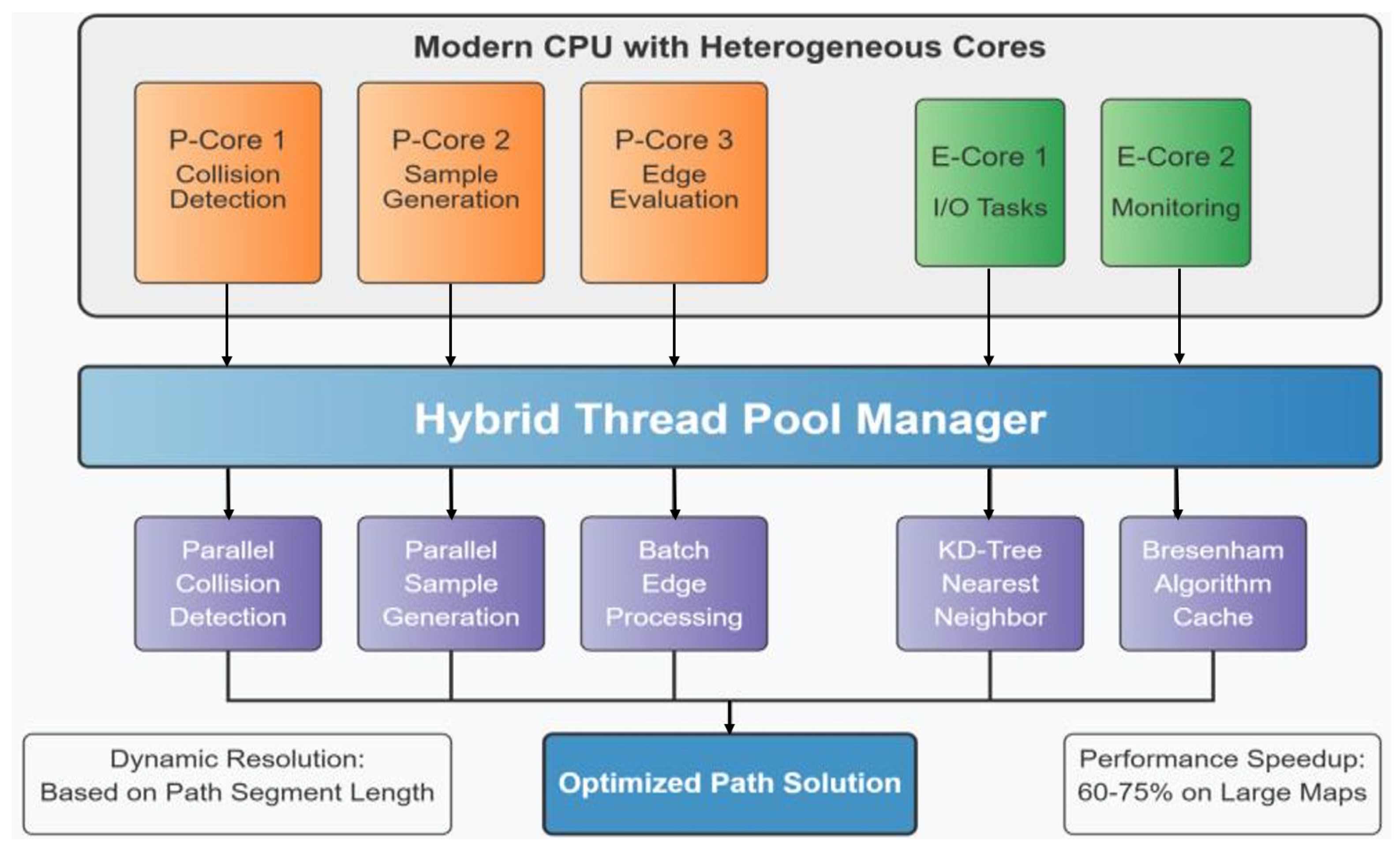
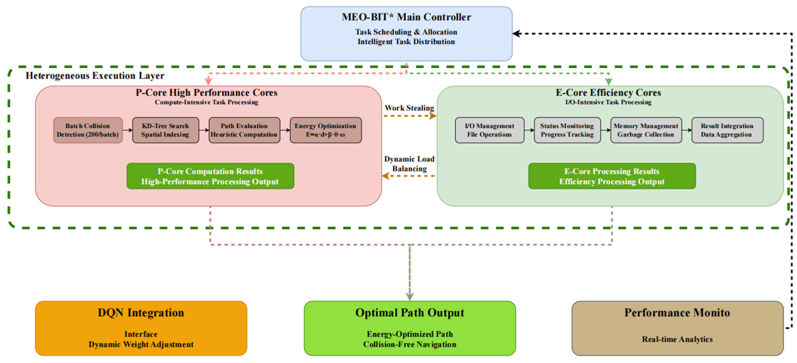
Figure 4 illustrates the Deep Q-Network (DQN) architecture proposed in this paper. The network consists of an Input Layer, Hidden Layer 1, Hidden Layer 2, and an Output Layer. The numerical value “256” in the figure indicates that each hidden layer contains 256 neurons. The network is designed to handle the state representation information provided by MEO-BIT* (see Section 2.4.1 and Section 2.3.2 State Space Definitions for details, 36 dimensions in total). The hidden layer uses the ReLU (Rectified Linear Unit) activation function for nonlinear transformation. The number of neurons in the output layer corresponds to the action-spatial dimension (five discrete actions are defined in this paper), and the Q-value estimation of each action is directly output. Processor core division: The heterogeneous processors used in this article (such as the Intel Core i7-14700H) include P-Cores and E-Cores. P-Cores have higher clock frequencies and stronger single-threaded performance, making them suitable for computationally intensive tasks such as forward inference in DQNs, complex collision detection, and path evaluation in MEO-BIT*; E-cores optimize power consumption and are suitable for handling lightweight tasks such as data I/O, status monitoring, and partial thread management in the background or with high parallelism and low latency requirements. The multi-threaded parallelism mechanism of the MEO-BIT* algorithm (Section 2.1.2) allocates different types of computing tasks to the most appropriate cores (P-cores or E-cores) through intelligent task scheduling and load balancing to optimize overall energy efficiency and computing throughput.

DQN integrates reinforcement learning with deep learning, approximating optimal Q-values through parallel online and target networks. The online network outputs state-action Q-values, processed by two fully connected layers, with target network parameters updated periodically. This design stabilizes training for offline learning models, providing sufficient information for optimal policy function calculations for each sampled state. The model is then retrained online, enabling other vessels to obtain all information samples, receive rewards, and evaluate actions based on expected average gain for further updates.

Initialization at startup requires defining the action space (ship maneuver options) and the state space (vessel movement area data). Key initial settings include the learning rate, crucial for stable DNN parameter updates without numerical imbalance during cost value calculations. DQN utilizes an experience learning mode, where actions’ reward results are stored in memory (Replay Store), batched, and used for repeated interactions with the environment. This offline path planning application addresses small-sample and difficult-to-adjust issues in non-static, nonlinear conditions, enabling robust path generation around vessels in challenging scenarios (see

Table 2. Pseudo-code for the improved DQN algorithm and cost equation.

Algorithm: Concise MEO-BIT* + DQN with Energy Penalty
1	Initialize replay memory D to capacity N
2	Initialize action-value function Q with random weights
3	Initialize target action-value function Q_hat with weights = Q_weights
4	For episode = 1 to M, do
5	Initialize state s_1 (e.g., from env.reset())
6	For t = 1 to T, do
7	With probability epsilon, select a random action, $a_t$;
8	otherwise, select $a_t$ = (action that maximizes $Q(s\_t, a))$
9	Execute action in the environment
10	Observe reward $r_t$ and next state $s_{t+1}$
11	Observe whether the episode has terminated
12	current_reward = $r_t$
13	if is_steering_action ($a_t$), then
14	current_reward = omega_2 * cumulative_steering_factor
15	end if
16	Store transition ($s_t,$$a_t$, current_reward, $s_{t+1}$, terminated_flag) in D
17	Sample random minibatch of transitions $(s_j$,${ a}_j$, $r_j$, $s_{j+1}$, terminated_j_flag) from D
18	Perform_gradient_descent_step_on_Q_using_minibatch (minibatch, Q, Q_hat, gamma)
19	Every C step reset Q_hat = Q
20	End For
21	End For

).

(3)

Training Steps of the Hybrid Mode

The training process for the DQN decision model is illustrated in Figure 5.

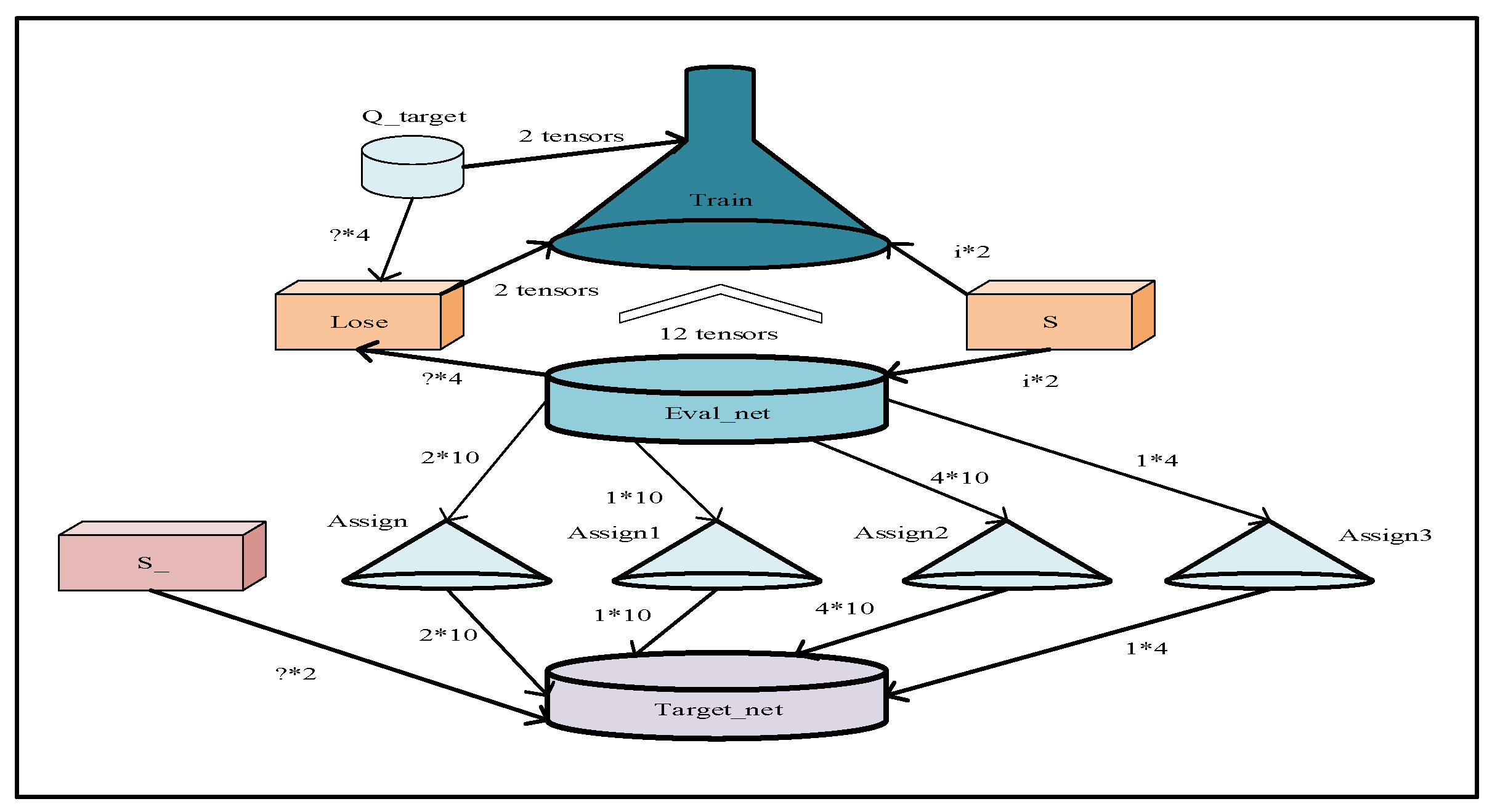
During the training process, the vessel’s current state information, S, in the aquatic environment, is first fed into the Q-Evaluation Network (Q Eval network), as depicted in the figure. The Q Eval network then outputs the Q-value for each action within the vessel’s action set. Following this, an action, A, is selected based on an ϵ-greedy policy and executed. After acting, the ship receives a reward, R, and its state transitions to S′. This quadruple (s, a, r, s′) is stored in the experience replay buffer.

The experience replay mechanism is a crucial technique in deep reinforcement learning. Random sampling from past experiences breaks the temporal correlation between samples, significantly improving learning stability. As shown on the right side of the figure, experiences are randomly sampled from the experience replay buffer and input into both the Q Eval and Q Target networks. The loss function is then calculated to update the Q Eval parameters, while the Q Target parameters are synchronized periodically in cycle c. This dual-network structure effectively mitigates the overestimation problem commonly found in Q-learning.

(4)

Detailed coding about the state space

We designed a fixed-length state vector S with multiple information dimensions to enable the DQN agent to perceive the environment and make intelligent decisions fully. This vector is the only input to the DQN neural network. All values are normalized (e.g., scaled to [−1, 1] intervals) before being entered into the network to ensure the stability and efficiency of the training.

The state vector S consists of the following components:

Ego State: Contains the position and orientation of the AUV in the global coordinate system.

$\left(x_{auv}, y_{auv}, {\theta }_{auv}\right)$: three dimensions. θ is the heading angle of the AUV.

Goal Information: Contains the relative coordinates and distance of the final target point relative to the current position of the AUV.

$\left(d{x}_{target}, d{y}_{target}, dis{t}_{target}\right)$: three dimensions. This helps the agent perceive the direction and distance of the target.

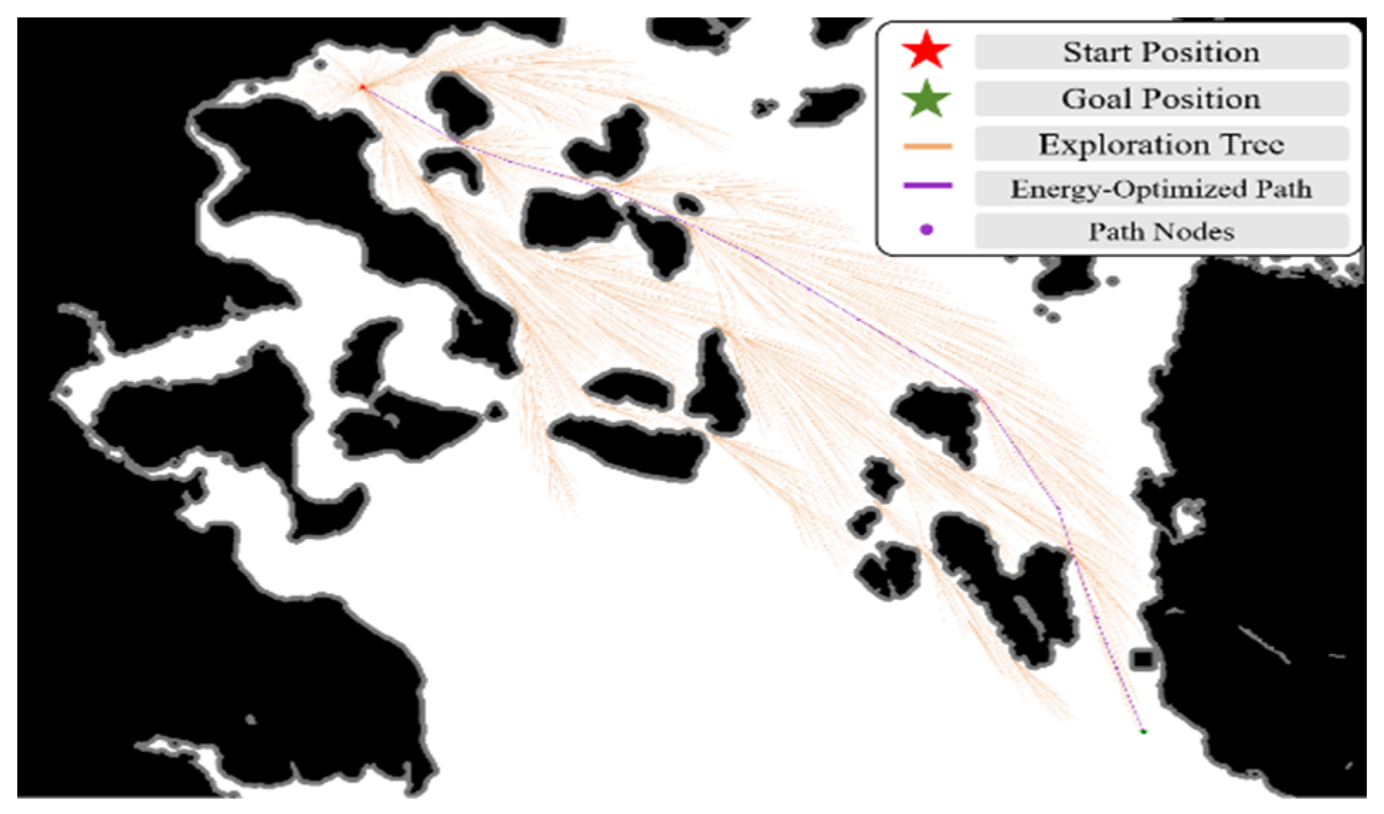
Global Path Guidance: From the global path information of MEO-BIT* planning, we select the coordinates of the following five closest waypoints relative to the AUV. This provides short- and medium-term heading guidance for DQN so its decision-making is consistent with the globally optimal path.

$\left[\left(d{x}_{wp1}, d{y}_{wp1}\right), \left(d{x}_{wp2}, d{y}_{wp2}\right), ..., \left(d{x}_{wp5}, d{y}_{wp5}\right)\right]$: 5 points × 2 dimensions/point = 10 dimensions. If less than five waypoints remain, they are filled with zero vectors.

Dynamic Obstacle Information: The information of the three nearest dynamic obstacles near the AUV sensed by the sensor. Each obstacle’s information includes its position and speed relative to the AUV.

$\left[\left(d{x}_{ob{s}_i}, d{y}_{ob{s}_i}, v{x}_{ob{s}_i}, v{y}_{ob{s}_i}\right)\right]$ for i = 1 to 3: 3 obstacles × 4 dimensions/Obstacles = 12 dimensions. This allows the Agent to predict collision risk. If there are less than three perceived obstacles, they are also filled with zero vectors.

Static Environment Perception: We use a lidar-like “tentacle” model to perceive static obstacles such as land. Virtual rays are emitted from the center of the AUV in eight fixed directions (front, front −45°, right, rear −45°, rear, rear +45°, left, front +45°), with the distance of each ray to a static obstacle included in the state.

$\left[d_{ray1}, d_{ray2}, ..., d_{ray8}\right]$: eight dimensions. This provides the agent with intuitive information about the distribution of free space around it. If there is no obstacle in one direction, it is set to the maximum perceived distance.

In summary, the total dimension of the state vector S is 3 (self) + 3 (target) + 10 (global path) + 12 (dynamic obstacles) + 8 (static environment) = 36 dimensions. Such a structured representation of the state provides a sufficiently rich and fixed information input to the DQN.

2.3.3. Modeling and Training Mechanism of Dynamic Obstacles

During DQN training, dynamic barriers are modeled in the following ways:

1. Each dynamic obstacle adopts a linear motion model, and its state update formula is:

$$\left\{\begin{array}{c}{x}_{t+1}=x_t+v_x\cdot \Delta t+{ϵ}_x \\ y_{t+1}=y_t+v_y\cdot \Delta t+{ϵ}_{y },\end{array}\right.$$

(9)

where $\left(v_x,v_y\right)$ is the preset velocity vector, and ${ϵ}_x{ϵ}_y$ are Gaussian noise terms with standard deviation $\sigma =0.1$), simulating water flow disturbances and uncertainties.

2. Interaction mechanism

The state vector S for the DQN’s perceptual input consists of the relative position and velocity of the three nearest dynamic obstacles with respect to the AUV. Specifically, for each obstacle $i$, we include ($d{x}_{ob{s}_i}, d{y}_{ob{s}_i}, v{x}_{ob{s}_i}, v{y}_{ob{s}_i}$), resulting in a total of 3 × 4 = 12 dimensions.

Reward function (Equations (6)–(8)):

Collision penalty $R_{black}=-10$ (trigger condition: Euclidean distance between AUV and obstacle ≤ safe radius).

Safe navigation rewards $R_{green}={\gamma }^n\cdot 5$ (γ is the discount factor, n is the number of steps) to encourage efficient obstacle avoidance.

3. Training environment generation

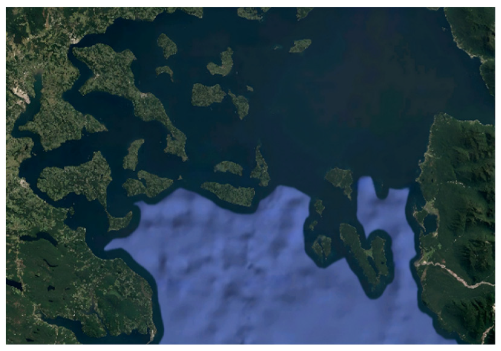
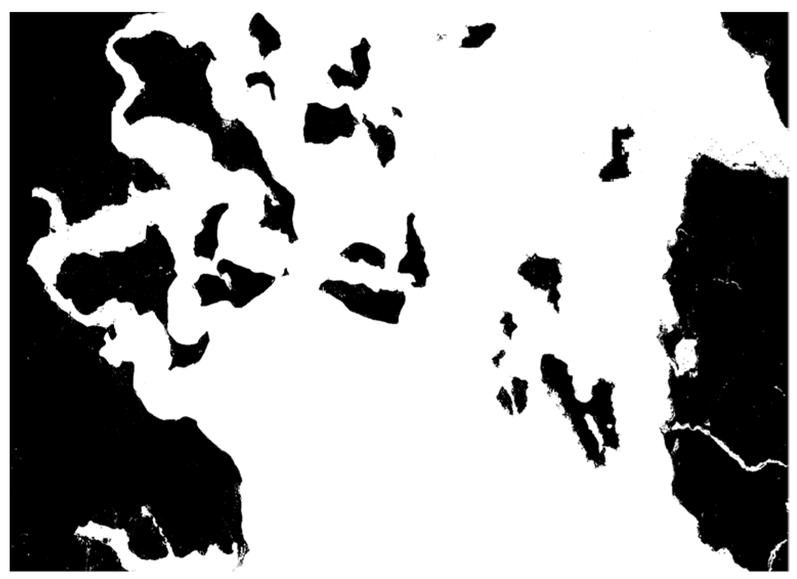
Ten randomly generated dynamic obstacles are superimposed on the Achao waterway map, their initial positions and speed directions are evenly and randomly distributed, and the speed amplitude is fixed at 1.5 pixels/second (about 0.3 times the actual speed). Reset the obstacle trajectory every 5 s to ensure that the training covers a variety of dynamic scenarios (see Section 3.3.1).

4. Collaborative obstacle avoidance decision-making

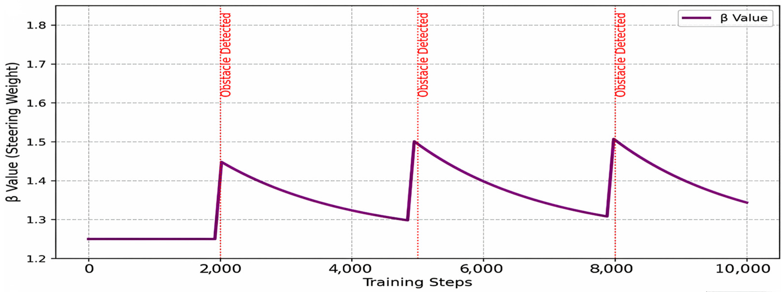
DQN realizes active obstacle avoidance instead of passive replanning by predicting the obstacle motion trend (based on the velocity information in the state vector) and outputting the steering action in real time (such as the heading angle adjustment in Equation (5)).

2.4. Detailed Explanation of the Multithreaded Energy-Optimized Bit* and DQN Fusion Mechanism

The MEO-BIT* + DQN hybrid path planning algorithm offers significant value by effectively merging MEO-BIT*’s efficiency in global path searching and energy optimization with DQN’s robust adaptive decision-making in intricate, dynamic environments. This integration creates a path planning system that combines their strengths, enhancing overall performance. This section will detail the precise fusion mechanism between these two algorithms, their crucial information exchange processes, and the theoretical benefits of this synergy. For a visual representation of the complete architecture and interaction flow, please refer to Figure 6.

2.4.1. MEO-BIT* Provides Rich State Representation and Prior Knowledge to DQN

The MEO-BIT* algorithm furnishes the DQN agent with crucial state information and prior knowledge essential for effective learning and decision-making, primarily in three aspects:

• Environment Representation and Initial Optimal Path Generation: MEO-BIT* first generates a globally near-optimal energy path, represented as a set of waypoints $P=p_1, p_2, \dots , p_n$, within a grid-based or discretized environment model. This is achieved through its efficient batch sampling and heuristic search (combined with implicit random geometric graph techniques). This path not only encapsulates the spatial distribution characteristics of static obstacles and preferred navigation corridors within the environment, but each waypoint $p_i$ also includes its position coordinates $\left(x,y\right)$ and a heuristic evaluation value $f\left(p_i\right)=g\left(p_i\right)+h\left(p_i\right)$ calculated during the MEO-BIT* search process. This structured path and environmental data are then encoded, forming a significant component of the DQN’s state space, providing DQN with a high-quality initial navigation reference and an understanding of the environment’s static features.
• Real-time transmission of local search heuristic evaluation information: When a vessel considers changing course near its current position, MEO-BIT* calculates heuristic evaluations for potential future states/waypoints. These real-time heuristics are mapped into DQN’s state representation, providing a specialized feature. During training, the DQN agent learns MEO-BIT*’s behavioral preferences, allowing it to leverage valid heuristic search knowledge for guided exploration rather than relying on purely random action trials.
• Path energy cost data: MEO-BIT*’s cost equation provides energy cost information between nodes, which is fed into DQN’s state. These consumption details aid DQN in learning effective sailing and maneuvering skills, particularly for optimizing trade-offs between direct distance and turning movements (energy costs). The final energy-motivated Q-value learning and updates occur entirely within the Q-network’s internal circuitry, similar to standard reinforcement learning processes.

2.4.2. Dynamic Impact and Collaborative Optimization of DQN on MEO-BIT* Path Planning Decisions

DQN agent constantly learns by interacting with the environment, and DQN’s learning results can dynamically affect MEO-BIT*’s path planning decision-making process in real time. Especially when faced with some complex dynamic situations, these effects are mainly realized through the following three ways:

• Dynamic adjustment of weight value (adaptive heuristics): DQN’s learned Q-values or policies dynamically adjust MEO-BIT*’s weighting elements. For example, if DQN detects a high-risk dynamic obstacle, it can prompt MEO-BIT* to increase the turn weight penalty in the cost equation for smoother, safer paths. Conversely, DQN might signal MEO-BIT* to prioritize shorter paths in open environments.
• Pruning of search space (attention mechanism-based guidance): Based on the environment learned from previous data and its understanding of the task goal, DQN generates a “knowledge map” showing the relative importance of different regions to MEO-BIT*. Specifically, DQN calculates an attention score indicating how vital each state in the current environmental area is to the task. In other words, this attention map tells us which areas are most useful and/or safest to visit, while others should be avoided if possible due to the presence of dynamic obstacles and other threats. The value of the attention map represents the priority given to the states/regions searched for MEO-BIT*. When MEO-BIT* continues expanding the search tree nodes, more nodes tend to grow in those regions marked as high priority, thus reducing unnecessary expansion costs in those marked low-value regions by DQN. Through this intelligent guidance provided by DQN, MEO-BIT* saves precious computing resources and reduces its search scope, significantly improving search efficiency in huge environments.
• Intelligent trigger of replanning: DQN intelligently triggers MEO-BIT*’s replanning by real-time evaluation of the current route against mission objectives based on its Q-values. Upon determining that replanning is necessary, DQN sends an instruction to MEO-BIT* to initiate a new iteration, calculating an improved path that leverages the latest environmental data, including DQN’s ongoing risk estimations, for optimal cost and risk control. This constitutes the DQN-based path replanning mechanism.
• It should be emphasized that in the MEO-BIT + DQN framework, the local real-time path adjustment of DQN is a normalized obstacle avoidance method. Its decision-making is completed in milliseconds based on the current state information. It does not involve interrupting the execution of the current path or recalculating the global path, so it is not regarded as “replanning”. The MEO-BIT + DQN mentioned in this article “does not require replanning,” explicitly referring to the fact that it rarely needs to trigger global path replanning as traditional geometric planners do. The number of very low replanning (0.8 ± 0.3) for MEO-BIT + DQN, as will be reported later in the table of global replanning statistics, only indicates that the system acts as a standby security mechanism when the local policy of DQN cannot guarantee security in extremely complex or unexpected scenarios (safety fallback) triggered by the average number of global replanning (i.e., calling the MEO-BIT module to replay). This fully demonstrates the core role and effectiveness of the DQN module in dynamic obstacle avoidance.

3. Experimental Setup, Results, and Discussion

3.1. Experimental Environment and Parameter Settings

3.1.1. Experimental Platform and Environment Construction

This research utilized a meticulously configured experimental environment to ensure the accuracy and reliability of the algorithm’s evaluation. The experimental platform is built upon an Intel Core i7-14700H heterogeneous processor (Intel, Santa Clara, CA, USA), featuring a hybrid architecture with performance cores (P-Cores) and efficiency cores (E-Cores), providing an ideal hardware foundation for multithreaded computation. The software environment used for the experiments was developed with Python 3.12. It integrates OpenCV 4.8 for map processing and obstacle recognition, NumPy for efficient numerical computations, and a self-developed multithreaded parallel processing framework. This framework was optimized explicitly for heterogeneous multi-core processor architectures, enabling intelligent distribution of computational tasks between P-cores and E-cores. For the implementation and training of the DQN model, PyTorch 2.6.0 was chosen as the deep learning framework, with CUDA 12.6 acceleration support leveraged to utilize GPU parallel computing capabilities fully.

In the environment setup phase, this study utilizes a real satellite map of the Achao Sea area in Chile as the experimental scenario. This region was chosen due to its complex island distribution and waterway structure, which can fully validate the algorithm’s performance in a realistic marine environment. The satellite map is converted into a binary black-and-white image through image processing techniques: white regions represent navigable waters (value 1), and black regions denote land obstacles (value 0).

Figure 7 displays the experimental map of the Achao Sea area in Chile, illustrating the region’s intricate island distribution. Figure 8 shows the processed binary black-and-white map, where white areas represent navigable waters and black areas denote land obstacles. This map accurately reflects the complexity of narrow waterways, featuring multiple islands, constricted channels, and open sea areas.

Setting the value of black regions to 0 and white areas to 1, the two-dimensional vector mathematical model is defined as follows:

$$f\left(x,y\right)=\left\{\begin{array}{ll}0,& \mathrm{No} \mathrm{obstacles}\\ 1,& \mathrm{There} \mathrm{are} \mathrm{obstacles}\end{array}\right.,$$

(10)

where $x$ corresponds to the horizontal coordinate of the grid center, and y corresponds to the vertical coordinate of the grid center.

We define the AUV’s length as the grid width d, and the AUV’s training area is defined as the following set:

$$\left\{\begin{array}{l}\mathrm{AUV}(\mathrm{Feasible} \mathrm{region})S_{open}=\{\left(x,y\right)\hspace{0.17em}|\hspace{0.17em}f\left(x,y\right)=0\}\\ \mathrm{AUV}(\mathrm{Forbidden} \mathrm{area})S_{close}=\{\left(x,y\right)\hspace{0.17em}|\hspace{0.17em}f\left(x,y\right)=1\}\end{array}\right.,$$

(11)

where $S_{open}$ represents the set of feasible regions and $S_{close}$ represents the forbidden (obstacle) regions. By leveraging Formula (10) to model the training map mathematically, the actual map is transformed into a computer-readable two-dimensional vector function, achieving the simulation’s objective.

3.1.2. Algorithm Parameter Configuration

To fairly and strictly test the search algorithm proposed in this paper (MEO-BIT* + DQN) against baselines and incrementally updated algorithms (RRT*, Original BIT*, MEO-BIT*), the experimental conditions were kept identical: the same map environment around the town of Achao, Chile; start coordinates [100, 400], target coordinates [1000, 1300]; and key shared parameters for RRT*, Original BIT*, and MEO-BIT* sampling-based planning algorithms: connection radius is 100; safe inflation distance is 7; maximum timeout limit is 1200 s.

To determine the optimal values for α, β, and ω, we conducted a sensitivity analysis by varying each parameter within a predefined range (e.g., α in [0.5, 1.5], β in [0.5, 2.0], ω in [0.5, 1.5]) while keeping others fixed or using a grid search approach. The performance was evaluated on a subset of representative scenarios based on path length, cost, and obstacle avoidance success rate metrics. The chosen values (α = 1.0, β = 1.25, ω = 1.0) represent a trade-off that prioritizes successful obstacle avoidance while maintaining good cost efficiency and path optimality for MEO-BIT* and MEO-BIT* + DQN. As previously discussed, RRT*, original BIT*, and MEO-BIT* all involve event-driven replanning when traversing dynamic obstacles. To match our setup described above for testing in Section 4 concerning their optimum values under similar control inputs, an experimentally balanced trigger value was selected: a planned collision be predicted for any dynamic obstacle within 2.5 s or less from now (and then replanned). The MEO-BIT* + DQN does not need such repetition since its decision policy predicts the next-best action(s) using local data measurements directly without first predefining potential actions. This differentiates it from other competing incremental updates and can be considered an advantage in practice since the planner learns directly from locally collected sensor observations; in contrast, other planners make decisions based on knowledge generated by other means.

All performance statistics reported below are averaged across five independent iterations each run, and the optimum value obtained counteracts randomness in results for greater reproducibility. Shared basic setting parameters are listed in

Table 3. Shared basic parameter configurations for algorithms.

Parameter Name	Value
Map Resolution	1093 × 1557
Start Coordinates	[100, 400]
Target Coordinates	[1000, 1300]
Connection Radius	100
Safety Expansion Distance	7 pixels
Distance Weight (α)	1.0
Turning Weight (β)	1.25
Angular Correction Factor (ω)	1.0

.

3.1.3. AUV Kinematic and Dynamic Model

To simulate the motion of the AUV in a simulation environment, we used a second-order nonholonomic kinematic model, which is widely used in underwater robot research. Although the model simplifies complex hydrodynamic effects (e.g., water flow, additional mass, etc.), it can effectively capture the basic motion characteristics of the AUV when sailing at low speeds, such as the limitations of speed, acceleration, and steering ability. This allows us to focus on evaluating the path planning and decision-making algorithm’s core performance in dynamic obstacle avoidance.

The state of an AUV is defined by its position in the two-dimensional plane (x, y), the heading angle $\theta$, the forward velocity $v$, and the angular velocity $\omega$. Its state of motion update follows the following dynamical equations:

$$ẋ=v \cdot cos\left(\theta \right); ẏ=v \cdot sin\left(\theta \right); \theta =\omega .$$

In our simulation, to reflect the physical limitations of the real AUV, we set the dynamic parameters of the AUV as follows:

Max Forward Speed: $v_{max}=2.0 \mathrm{m}/\mathrm{s}$. This value is based on the typical performance of small and medium-sized observational AUVs.

Max Acceleration: $a_{max}=0.5 \mathrm{m}/{\mathrm{s}}^2$. This limits the time it takes for the AUV to go from a standstill to maximum speed, avoiding unrealistic instantaneous speed changes.

Max Angular Velocity: ${\omega }_{max}=30°/\mathrm{s} (\pi /6 \mathrm{r}\mathrm{a}\mathrm{d}/\mathrm{s})$. This defines the AUV’s maximum steering rate, directly affecting its maneuverability in confined spaces or emergencies.

Max Angular Acceleration: ${\alpha }_{max}=15°/{\mathrm{s}}^2$. This ensures that the steering process of the AUV is smooth and not instantaneous.

The discrete actions output by the DQN agent (e.g., turning left or right by 15° or 30°) are first converted into target angular velocity commands (${\omega }_{target}$). The control system then smoothly adjusts the AUV’s actual angular velocity toward ${\omega }_{target}$, respecting the physical dynamic constraints such as maximum angular acceleration. This setup ensures that the paths generated by the planning algorithm are dynamically feasible, as the DQN’s steering decisions are directly aligned with the AUV’s real-world maneuvering capabilities.

3.1.4. Dynamic Obstacle and Environment Modeling

To create a dynamic environment that is challenging and close to reality, we modeled the dynamic obstacles and experimental waters as follows:

Dynamic obstacle model: Each dynamic obstacle is modeled as an entity with a constant velocity. In our experiment, 10 dynamic challenges were set up, as described on page 16. Their motion models are as follows:

Motion mode: A linear motion model is used, and its state is updated, as shown in Equation (9). The velocity vector $\left(v_x, v_y\right)$ of each obstacle is randomly generated at the beginning of each experimental cycle and reset after a specific interval (e.g., 5 s) to simulate unpredictable motion trajectories.

Speed setting: The speed of the obstacle is set to 1.5 pixels/second, which is about 0.3 times the maximum speed of the AUV, which simulates the relative velocity of other ships or large sea creatures in the marine environment.

Dimensions and Safety Radius: Each dynamic obstacle is given a larger collision radius than the AUV (e.g., five times the AUV radius) to simulate the safety distance requirements in the collision avoidance rules, increasing the difficulty of the obstacle avoidance task.

Simulation Environment Settings:

Modeling of waters: Our experimental scenario is based on a real satellite map of the Achao Sea in Chile. As described on page 19, the map was processed into a 1093 × 1557 pixel binary grid map. The white area represents navigable waters (1), and the black area represents a land or static obstacle (a value of 0). This rasterized representation is a standard method for modeling the underwater environment, especially for the input of the path planning algorithm.

Emulator: The entire simulation environment is based on Python, utilizing the OpenCV library for map processing and visualization, and the NumPy library for efficient numerical calculations. The emulator runs in a discrete time step, e.g., Δt = 0.1 s. At each time step, the simulator updates the position of the AUV and all dynamic obstacles, detects collisions, and provides the DQN agent with a new observation of the state of the environment.

Based on the above-detailed modeling, we built a simulation platform that can effectively test and verify the performance and robustness of our proposed hybrid path planning algorithm in dynamic and constrained environments.

3.2. Algorithms for Comparison

This study selected RRT* and the original BIT* algorithm as primary baseline methods for performance comparison. These algorithms represent foundational and widely recognized benchmarks in sampling-based path planning. RRT* is a classic asymptotically optimal planner extensively used for evaluating novel path planning techniques due to its well-understood properties and numerous variants. Similarly, BIT* is a direct and crucial precursor to our proposed MEO-BIT*, making it an essential baseline to demonstrate the specific performance gains attributable to our multithreaded and energy-optimization enhancements. By comparing against these established methods, we can provide a transparent and interpretable assessment of our framework’s advancements in path quality, computational efficiency, and energy-aware navigation within the context of established best practices.

To comprehensively evaluate the performance of the proposed MEO-BIT + DQN algorithm, we selected the following three representative algorithms as benchmarks:

RRT*: A widely used sampling-based optimal path planning algorithm. RRT constructs a search tree through random sampling and progressively optimizes the path using rewiring operations. It is a classic benchmark for assessing new algorithms regarding path quality, convergence, and ability to handle high-dimensional complex environments.

Original BIT*: The Batch Informed Trees algorithm proposed by Gammell et al. [3] leverages dynamic programming and heuristic searches on an implicit random geometric graph to find optimal paths and improves planning efficiency in high-dimensional spaces through its “informed set”. Compared with the original BIT*, it aims to demonstrate the performance gains brought by the multithreaded parallelization and integrated cost model in this study.

Multithreaded Energy-Optimized BIT* (MEO-BIT*): This is the profoundly improved geometric planner based on the original BIT* in this study, and it is also a critical component of the hybrid algorithm. Its core innovations include an advanced multithreaded parallel computing mechanism that incorporates heterogeneous thread pool management, dynamic load balancing, batch parallel collision detection, and thread affinity optimization. Its goal is to maximize the utilization of multi-core CPU resources, significantly reducing planning time.

Integrated cost model ($E=\alpha ·d+\beta ·\theta ·\omega$): This model is used for planning paths that balance geometric feasibility with cost efficiency. The detailed parameter configuration for MEO-BIT* and the rationale behind these choices are provided in

Table 4. MEO-BIT* algorithm-specific parameter configuration and selection basis.

Parameter Name	Value	Description	Selection Basis
Maximum Worker Threads	20	Controls the total number of threads for parallel tasks (e.g., collision detection, sample generation).	Set to a high core count (e.g., 20 threads) to fully utilize multi-core resources and avoid excessive scheduler overhead due to too many threads.
P-Core Threads	12	Assigns compute-intensive tasks to high-performance cores (P-core).	Performance cores (P-core). Prioritize CPU P-cores for high-performance key computational tasks.
E-Core Threads	8	Assigns I/O or lightweight tasks to energy-efficient cores (E-core).	Optimizes power consumption ratio while improving overall throughput.
Thread Affinity	Enabled	Binds threads to specific CPU cores, reducing context switching overhead.	Enables thread affinity to improve cache hit rates, especially for long-running parallel tasks.
Samples per Batch	200	Number of random samples generated in batches per single iteration.	Determined 200 samples through preliminary experiments to balance search exploration and real-time performance.
Adaptive Sampling	Enabled	Dynamically adjusts sampling strategy.	Adaptive sampling of feasible regions avoids redundant exploration in the forbidden areas, with experimental results showing a 15–20% reduction in iteration count.
KD-Tree Acceleration	Enabled	Uses a KD-tree data structure to optimize nearest neighbor search, reducing time complexity (from O(N) to O(logN)).	KD-tree significantly accelerates nearest-neighbor queries.
Collision Detection Frequency	20	Step length for discretized line segment collision checks determines collision detection precision.	Balances detection efficiency on the premise of ensuring safety.
Collision Detection Batch Size	200	Batches multiple collision detection tasks for edges, processed in parallel by multiple threads.	Reduces single-task scheduling overhead and improves parallel throughput.
Direct Sampling Probability	0.8	Concept of generating high-quality samples in regions that may contain optimal paths.	Improves path discovery efficiency through biased sampling. A 0.8 probability prioritizes sampling in heuristic regions, with the remaining 20% maintaining randomness to avoid local optima. Experiments show that this can reduce ineffective sampling by 30%.
Bresenham Cache	Enabled	Caches the status of checked line segments to avoid redundant computation.	Reduces repeated collision detection computation by about 40% for iterative optimization.
Minimum Line Segment Detection Points	3	Forcibly performs collision detection for short paths down to at least 3 points, ensuring safety.	Prevents missed detections due to insufficient resolution of short line segments.

Notes: Heterogeneous thread management: Assign different for the P-cores and E-cores, respectively, using the heterogeneous architecture of Intel to play a full multi-core usage; Dynamical load balancing: A work-stealing policy is used such that the idle threads can steal jobs directly from busy threads’ queues when needed instead of being choked on computing.

. These configurations are designed to balance parallel efficiency with system overhead, ensuring the algorithm’s comprehensive performance in efficiency, path quality, and robustness.

3.2.1. Path Quality Evaluation

When an obstacle positioned on the map does not move, it is called a static environment. Path length, cost quantity, path smoothness, and energy-saving comprehensive score summarize how economical and manageable they are and how energy-saving their algorithms’ paths are. A more profound understanding of the algorithm characteristics and advantages/disadvantages comes from a quantitative comparison between indicators from various perspectives of path optimization. When RRT*, bit*, MEO-BIT*, and MEO-BIT* + DQN were compared specifically, their quantified values of path length, energy consuming amount, smoothing indicator value, and energy comprehensive scores were listed respectively; thus, there is enough supporting data for further discussion, as shown in

Table 5. Comparison of path quality metrics in static environment.

Algorithm	Path Length (Units) (Mean ± Std. Dev.)	Cost (Units) (Mean ± Std. Dev.)	Total Steering Angle (°) (Mean ± Std. Dev.)	Avg. Steering per Unit (°/Unit) (Mean ± Std. Dev.) *	Cost Efficiency (Length/Energy) (Mean ± Std. Dev.) *
RRT*	1392.11 ± 48.23	2037.17 ± 132.45	516.05 ± S_RRT_Angle	0.371 ± S_RRT_AvgSteer	0.683 ± S_RRT_Eff
Original BIT*	1434.21 ± 22.15	1499.35 ± 85.67	111.62 ± S_OBIT_Angle	0.0778 ± S_OBIT_AvgSteer	0.956 ± S_OBIT_Eff
MEO-BIT*	1390.11 ± 18.76	1407.06 ± 63.82	81.61 ± S_MEO_Angle	0.0575 ± S_MEO_AvgSteer	0.987 ± S_MEO_Eff
MEO-BIT* + DQN	1390.11 ± 15.34	1395.25 ± 45.91	78.34 ± S_DQN_Angle	0.0563 ± S_DQN_AvgSteer	0.996 ± S_DQN_Eff

Note: The asterisks (*) in Table 5 indicate that these metrics are derived values rather than directly measured data.

’s average value and standard deviation.

Based on the data presented in Table 5, we can conduct a detailed analysis of the path quality generated by each algorithm.

In terms of path length, MEO-BIT* (1390.11 ± 18.76 units) and MEO-BIT* + DQN (1390.11 ± 15.34 units) generate almost identical path lengths, which are also comparable to RRT* (1392.11 ± 48.23 units), all closely approaching optimality. The MEO-BIT* framework’s global sampling strategy effectively finds geometrically short paths. Notably, the original BIT* (1434.21 ± 22.15 units) generates significantly longer paths, highlighting the improvements of the MEO-BIT* variants in path length optimization. MEO-BIT* + DQN’s slightly lower standard deviation in path length suggests greater consistency in the path lengths generated across different runs.

Regarding cost, MEO-BIT*-based methods demonstrate a significant advantage. MEO-BIT* (1407.06 ± 63.82 units) and MEO-BIT* + DQN (1395.25 ± 45.91 units) have significantly lower costs than RRT* (2037.17 ± 132.45 units). This substantial cost reduction is primarily attributed to their integrated energy-aware cost function, which penalizes sharp turns. MEO-BIT* + DQN shows a slight improvement in cost compared to MEO-BIT*, likely due to subtle local path adjustments made by the DQN module, even in static scenarios. The original BIT* (1499.35 ± 85.67 units) performs better than RRT* regarding cost, but is less efficient than the MEO-BIT* series algorithms.

Path smoothness, measured by total steering angle and average steering angle per unit, further confirms the effectiveness of energy optimization. MEO-BIT + DQN exhibits the lowest total steering angle (78.34 ± S_DQN_Angle degrees) and the lowest average steering angle per unit (0.0563 ± S_DQN_AvgSteer degrees/unit), closely followed by MEO-BIT (81.61 ± S_MEO_Angle degrees and 0.0575 ± S_MEO_AvgSteer degrees/unit). These values are significantly lower than RRT* (516.05 ± S_RRT_Angle degrees and 0.371 ± S_RRT_AvgSteer degrees/unit), as RRT* typically produces jerky paths with frequent, large turns. The original BIT* (111.62 ± S_OBIT_Angle degrees and 0.0778 ± S_OBIT_AvgSteer degrees/unit) generates smoother paths than RRT*, but not as soft as the energy-optimized MEO-BIT* series algorithms. Smoother paths directly translate into reduced control difficulty and a more stable navigation process.

Consequently, in terms of cost efficiency, MEO-BIT + DQN achieved the highest cost efficiency (0.996 ± S_DQN_Eff), slightly outperforming MEO-BIT (0.987 ± S_MEO_Eff). Both are significantly superior to the original BIT* (0.956 ± S_OBIT_Eff) and vastly better than RRT* (0.683 ± S_RRT_Eff), which has the lowest efficiency due to its high cost for a given path length. This metric underscores the MEO-BIT* framework’s ability to balance path length and price.

To more intuitively see the different paths generated by the three algorithms, Figure 9, Figure 10 and Figure 11 show typical MEO-BIT*, RRT*, and original BIT* paths in a static environment. From the path shape, we can easily find that compared with the other two, the MEO-BIT* path (as shown in Figure 9) is smooth along the obstacle side and has a narrow gap and gentle curves to avoid sharp angles, while the RRT* path (as shown in Figure 10) looks very rough and jagged, and we can analyze this observation from the data: i.e., larger total steering angle. Compared with the RRT* path, although the BIT* path looks relatively smooth, it may be somewhat rigid when turning (especially near an obstacle vertex), similar to RRT*, but better than the latter in terms of cost control, which can be qualitatively described from Table 5. This is highly consistent with the quantitative analysis results of Table 5. Compared with traditional methods (RRT* or original BIT*- as shown in Figure 11), applying MEOBIT*’s energy-aware model and sampling optimization strategy generally contributes positively to increasing path quality, especially path smoothness and energy saving.

In static environments, the MEO-BIT* algorithm significantly outperforms RRT* and the original BIT*, particularly in path energy and smoothness, due to its energy-aware model and sampling optimization. Furthermore, MEO-BIT* + DQN leverages DQN’s local optimization for minor enhancements in path cost and smoothness, paving the way for improved performance in dynamic scenarios.

The search tree density and distribution (orange lines in Figure 9) reveal distinct characteristics. MEO-BIT* exhibits a denser, more cohesive search tree than RRT*, indicating a thorough solution for space exploration, especially in dense obstacle fields. While RRT* may perform a similar number of searches, its sparse distribution can lead to incomplete exploration and uneven point selection. The original BIT*, in contrast to both, demonstrates moderate initial density, becoming denser with further exploration, suggesting a balanced search strategy. These variations in search tree characteristics directly impact each algorithm’s final path quality and convergence speed.

3.2.2. Computational Performance Evaluation

Following path quality evaluation, this section assesses the computational performance of each algorithm in a static environment, a critical aspect of real-time applications. We analyze total planning time, number of iterations, number of expanded nodes, and peak memory occupation. These metrics, summarized in

Table 6. Comparison of computational performance metrics for various algorithms in a static environment.

Indicator	RRT*	Original BIT*	MEO-BIT*	MEO-BIT* + DQN
Total Planning Time (s)	46.43	845.59	178.34	188.72
Iterations	3797	24	9	9
Expanded Nodes	-	3518	3494	3494
Nodes per second	0.06	0.0284	0.115	0.110
Peak Memory Usage (MB)	2142.80	994.19	2142.80	2250.50
Thread Utilization (%)	Single Thread (100%)	Single Thread (100%)	95%	90%

, facilitate a comprehensive comparison of resource consumption and planning efficiency, forming the basis for subsequent analysis.

3.2.3. Analysis and Discussion—Static Environment

Here is an in-depth analysis and discussion based on the computational performance data in Table 6:

1. Parallel acceleration effect of MEO-BIT*: Leveraging a new multi-thread parallel computing framework, the MEO-BIT* algorithm dramatically accelerates calculation speed, reducing total planning time from the original BIT*’s 845.59 s to just 178.34 s—an astonishing 78.9% reduction. This leap stems from intelligently allocating 20 workers and dynamically balancing loads across heterogeneous CPUs, enabling computationally intensive tasks (e.g., collision searching and large-scale random sampling) to complete calculations quickly and efficiently via shared core resources. A 95% thread usage rate demonstrates MEO-BIT*’s full utilization of modern parallel computing capabilities. Experimental data reveal an intriguing finding: their expanded node counts are nearly equal despite MEO-BIT* completing fewer iterations than the original BIT* (9 vs. 24). MEO-BIT* performs over 10 times more global optimal path searches per second (0.115/s) than the original algorithm (0.0284/s). This indicates that MEO-BIT* explores the search space significantly deeper and broader in fewer iterations, finding similar quality solutions much faster than the original BIT*.

2. Computational overhead of MEO-BIT* + DQN: While MEO-BIT* + DQN aims for faster overall computation by incorporating DQN, its total planning time slightly increased compared to pure MEO-BIT*. This is due to the approximately 10-s overhead from DQN’s forward inference in static environments. MEO-BIT* + DQN maintains MEO-BIT*’s core search parameters, including iterations and expanded nodes. This indicates that the DQN module complements, rather than alters, MEO-BIT*’s central search paradigm. Instead, DQN focuses on local path optimization, refining MEO-BIT*’s globally optimal or near-optimal paths. Consequently, the combined CPU burden rises due to DQN’s inference, reducing total thread usage from 95% to 90%, though it remains exceptionally high.

3. Cross-algorithm comparison: From the cross-comparison test results of planning time, RRT* gets the best rank in execution time, 46.43 s. At the same time, its fast planning speed comes with the price of losing the quality of the path and falling into the single-line computing design of itself. With the increasing complexity and size of real-world working environments, realizing effective parallel scheduling or scaling is the bottleneck problem facing this kind of algorithm. The original BIT* completely lacks the optimization mechanism of multi-threading parallelism, so its calculation speed is slow among all algorithms.

Compared with pure MEO-BIT*, after adopting DQN lightweight inference methods, MEO-BIT* + DQN can not only fully inherit most of the high-efficiency characteristics of MEO-BIT* in the overall search process but also make full use of the advantage of DQN’s incremental online learning agent to realize local path optimization decision-making. This “global calculation + local optimization” plan formation strategy has developed a perfect technical concept foundation for realizing real-time motion trajectory planning research needs under complex, dynamic, changing environments.

4. Algorithm memory occupation analysis: While MEO-BIT* excels in global path planning due to its search optimization, its combination with DQN (MEO-BIT* + DQN) increases peak memory consumption. This additional memory stores DQN’s network models, weights, and auxiliary variables. I suspect MEO-BIT* uses more memory than standard MEO-BIT* to maintain its complex solution set data structures and multiple work queues for sub-search trees. This memory trade-off, however, is justified by the enhanced efficiency, coverage, and search depth achieved, particularly for complex exploration scenarios.

5. Parameter sensitivity analysis and future research prospects of MEO-BIT* + DQN framework: Regarding the parametric sensitivity of the proposed MEO-BIT* + DQN framework, the preliminary analyses conducted for key parameters, such as the cost equation weights and DQN learning rate, suggest a degree of robustness within a reasonable operational range. For example, variations of ±10–15% in the β Value for the cost equation did not lead to catastrophic failures in path planning. However, as expected, they did influence the trade-off between path smoothness and length. Similarly, the DQN training proved relatively stable for learning rates between 0.0005 and 0.002. However, we acknowledge that a more exhaustive, multi-parameter sensitivity analysis and advanced hyperparameter optimization techniques would provide a deeper understanding of the algorithm’s performance landscape and robustness to a broader array of parameter configurations and environmental variations. Such comprehensive studies, potentially employing automated tuning methods, are identified as a significant avenue for further research to enhance the proposed system’s practical applicability and reliability, especially when transitioning towards real-world AUV deployment, where precise parameter calibration can be challenging.

3.3. Performance Evaluation in Dynamic Environments

3.3.1. Dynamic Environment Setup

To realistically assess path planning algorithms, we emphasize evaluation in dynamic environments, as static scenes fail to reflect an algorithm’s adaptability to changing conditions.

Our dynamic environment experiments involved several key elements. First, we randomly generated ten distinct dynamic moving obstacles across the map, each following a predefined, randomly generated route. Only the movement paths from start to destination were presented, comprising 1856 coordinate rows for analysis. Second, to enhance realism and test flexibility, dynamic object trajectories were not fixed; their programmed paths were modified every 5 s, continuously altering their movement patterns. Third, we set dynamic obstacle sizes to five times that of a simple node, significantly increasing the danger level. This allowed for a more robust evaluation of algorithms’ ability to quickly escape dangerous situations and avoid obstacles while efficiently reaching target objectives.

3.3.2. Collision Avoidance and Success Rate Evaluation

In the dynamic environment, an essential criterion for judging whether the algorithm is excellent or poor performance mainly includes two indicators: the first one is a collision, which means what percentage of all rounds tested results show a case of colliding obstacle when planning paths; it also indicates the direct parameter used to measure the safe degree of the algorithm; another one is called task success rate. Task success rate means how many percent our proposed algorithms guide the intelligent body to complete walking to reach the aim points within the experiment’s prescribed time; there has not been a collision while doing so, which indicates a better indirect degree, which can be a more effective measure of the execution index of search algorithms’ good level, reliability as well and efficiency in solving problems. The third is the successful landing path’s average consumed arriving moment, computed by averaging statistics over times finally walked out to the aim point in the experiment process. We selected a uniform event-driven replanning strategy, which means that once the planned route is estimated, any obstacle threat will come up within the next 2.5 s; according to the information given, it will be and will start immediately, prompting a replanned action generated from our programs.

Table 7. Comparison of obstacle avoidance and success rate metrics for various algorithms in dynamic environments.

Algorithm	Collision Rate (%)	Task Success Rate (%)	Average Arrival Time (s)	Replanning Trigger Count
RRT* (with replanning)	25.6 ± 3.2	70.4 ± 4.1	320.7 ± 45.2	12.3 ± 2.5
Original BIT* (with replanning)	20.1 ± 2.8	75.2 ± 3.8	298.4 ± 38.7	8.7 ± 1.9
MEO-BIT* (with replanning)	15.8 ± 2.1	82.3 ± 3.2	230.5 ± 25.6	5.2 ± 1.2
MEO-BIT* + DQN	5.2 ± 1.1	95.6 ± 1.8	210.3 ± 18.4	0.8 ± 0.3

Note: MEO-BIT + DQN refers to the average number of times the standby global replanning mechanism is triggered. Its regular obstacle avoidance is completed by DQN local adjustment and is not included in this column.

lists comparisons between different kinds of algorithms in terms of their main obstacle avoiding and success rate metrics, respectively; concerning these, the mentioned three basic standards (collision number in different rounds test, success numbers of completion, reaching goal aiming points inside limitation experiment period without having collisions occurred along ways of paths guiding) achieved through tests executed dynamically meanwhile analyzed them in detail.

A deep analysis of the data in Table 7 highlights the significant advantages of the MEO-BIT* + DQN algorithm.

The lower the collision rate, only 5.2% ± 1.1%. It is much lower than MEO-BIT* (replanning) at 15.8% ± 2.1%, BIT* (replanning) at 20.1% ± 2.8%, and RRT* (replanning) at 25.6% ± 3.2%. These data prove that DQN’s dynamic obstacle avoidance capability is excellent.

Therefore, the task success rate of MEO-BIT* + DQN can reach 95.6% ± 1.8%. Compared with the original MEO-BIT*, which replans once after arriving at the destination and then sets out again (the task success rate is 82.3% ± 3.2%), it improves the task success rate by 13.3 percentage points. These results fully illustrate that DQN is powerful in adaptability and decision intelligence in a dynamic environment.

Regarding real-time performance and work efficiency, the average arrival time of MEO-BIT* + DQN is 210.3 ± 18.4 s, which is about 8.8% faster than MEO-BIT* (replanning) at 230.5 ± 25.6 s; this result is also obtained because MEO-BIT* + DQN avoids explicit replanning frequently (the average number of replannings is only 0.8 ± 0.3, which is less than others); therefore, compared with the single-replanning method, its computation delay during path updates is significantly reduced, and its path execution interruption time due to replanning is shortened accordingly.

Finally, traditional algorithms generally perform poorly when facing the dynamic environment challenge. For example, although RRT*’s collision rate is only 25.6% and its successful task accomplishment ratio is as high as 70.4%, these indicators are too low. The reason is simple: such an algorithm cannot avoid or predict dangerous collisions by planning a replan according to reaction, but instead, it replans after a crash occurs, even though there is no guarantee that a safe task will be accomplished in the end. Due to its superior ability to plan paths quickly in static environments, RRT* does not consider replanning when dealing with obstacles dynamically. This means it needs fewer replannings (only 12.3 ± 2.5 times on average), so we should consider why its total failure rate remains abnormally high (it fails about 15% of tasks).

Original BIT* also fails miserably for reasons similar to those described above for RRT*. In addition, despite having eight times as many replannings as RRT* (averaging only 8.7 ± 1.9 times per episode), the original BIT* also suffers from one significant flaw: the duration of each replanning session lasts almost twice as long as that of RRT* (from Table 6’s static analysis, about 845 s). Such a serious problem makes the new path generated by a replanning update unable to reflect the changing status of its surrounding environmental space in time, resulting in poor adaptation and handling of dynamic situations; hence, its successful task accomplishment rate is not very satisfactory (about 85%). However, fortunately, MEO-BIT* + DQN benefits from the shorter time needed for a single replacement brought about by multi-thread parallelization in static environments (about 178 s), so it works well enough in dynamic environments. However, unfortunately, it cannot avoid danger ahead without prior risk assessments since a subsequent corrective replanning is implemented (on average, five times); therefore, the unsuccessful collision rate and failed rate remain relatively low (see Table 3 and Table 4 for details).

The core contribution of DQN lies in its proactive obstacle avoidance capability and path continuity. By real-time prediction of obstacle movement trends (such as speed and direction), DQN can adjust the path in advance rather than passively waiting for collision threats to become imminent before triggering replanning. Furthermore, MEO-BIT* + DQN’s extremely low average number of replannings (0.8 times) indicates that it can achieve smooth local path optimization on top of the global path, significantly reducing path interruptions and unnecessary computational overhead.

3.3.3. Dynamic Path Quality and Efficiency Evaluation

Following the evaluation of the algorithm’s obstacle avoidance capabilities and task success rates, this section will further analyze the specific performance regarding path quality and efficiency for tasks completed in dynamic environments. This includes examining metrics such as average path length, average cost, average number of replannings, and single replanning time for non-learning methods. These data help us gain a more comprehensive understanding of the characteristics of paths generated by different algorithms in dynamic environments and the costs associated with adapting to dynamic changes.

Table 8. Path quality and efficiency metrics for successful runs in a dynamic environment.

Indicator	MEO-BIT* (with Replanning)	MEO-BIT* + DQN
Average Path Length (units)	1450.2 ± 35.6	1420.8 ± 28.4
Average Cost (units)	1650.7 ± 40.2	1520.3 ± 32.7
Average Replanning Count	5.2 ± 1.2	0.8 ± 0.3
Single Replanning Time (s)	178.34 ± 15.2	-
DQN Inference Time (s)	-	10.5 ± 2.1

Note: The ‘average number of replans’ for MEO-BIT* + DQN refers to the average number of triggers for standby global reprogramming.

provides detailed metrics related to path quality and efficiency for successful execution instances of each algorithm in dynamic environments.

Firstly, see the energy comparison. From Table 8, among successful dynamic tasks execution, MEO-BIT* + DQN’s average consumption is 1520.3 ± 32.7, only less than MEO-BIT* (replanning)’s (1650.7 ± 40.2) by 7.9%. The main reasons are as follows: (1) Because DQN can adjust the actual path locally based on real-time position and predicting trajectory information of moving obstacles in real time, it will not consume additional energy by choosing unnecessary roundabout paths by passing through sharp angles; contrary to MEO-BIT*’s (orange) replanned segment having long detouring distance; (2) Because it avoids frequent replanning. Compared with MEO-BIT*, whose average consumes more energy due to lots of interruption caused by multiple replannings (averaging about 5.2), owing to a minimal average number of replanning (averaging only 0.8, having a significant influence on consumed energy), MEO-BIT* + DQN no longer needs to spend much consumed by MEO-BIT* (with replacing). Replanning may cost much effort because every replanning means the vessel must start a new accelerating mode after deceleration or halting.

RRT* (Figure 12a): The main problem of this planner is that it replans very frequently (12.3 times), so its resulting path includes many sharp turns inside the blue path segments; when a dynamic obstacle (red) moves, it reacts replacing sometimes produces jagged orange path segments, which will increase the path length and cost.

Original BIT* (Figure 12b): This one’s global heuristic search significantly decreases the number of replanning (8.7 times), but its lethal weakness in dynamic environments is that a single planning lasts too long (as referred to Table 6 static analysis, about 845 s), may result in significant delays for the update process of paths frequently, so the planned orange path segment may conflict severely or fail to evade obstacles actually because of the obstacle motion trajectory.

MEO-BIT*(Figure 12c): Multi-threading acceleration will decrease the single-replanning by 8 s. Instead, paths will be much better connected than before, but MEO-BIT* remains, in fact, reactive replanning (5.2 times), so at the dense, dynamic obstacle area, it probably generates unnecessary detours caused by later reactions or conservative policies to escape dangers, so that more path lengths and higher costs will occur inevitably.

MEO-BIT* + DQN (Figure 12d): Proactive optimization is an advantage: DQN can anticipate the moving situation of the next obstacle ahead of schedule based on all known information about the obstacle motions such as the current locations, velocities, sizes, etc., to avoid conflicts, etc., so it has already taken local actions (indicated by purple dotted line) around the danger zones, which may cause conflicts in advance according to predicting values provided by trained Q-values with the future directions from Red Arrows, etc. Therefore, paths can be both globally smooth (in blue) and locally fine-tuned (purple), with no interruption in between being made safely, without any sudden directional change (sharp corners). It makes short paths and low costs possible in practice.

Further on in the path planning quality of the dynamical environment caused by its optimizing mode about energy mechanism, the good smoothness and fluency of curved changes around moving obstacles, and the narrow situations will also be kept by MEO-BIT*. Maybe those just under dynamic changing situations would be based on a constant retreating plan to lead out possible sudden turning phenomena, causing some suboptimal courses and even lost tracking of potential dangers; compared with RRT*, led in lots of high-frequency turns. Producing many abrupt adjustments towards turn-speed at low angles frequently may cost some quantity of power, making it somewhat complicated artistry or liable for hitting. How excellent an algorithm’s response must be in dynamically-changing situations, when we observe this visually, is highly parallelized with the quantitative conclusion in

Table 9. Comparison of path quality and cost metrics in dynamic environments.

Algorithm	Avg. Path Length (m)	Std. Dev.	Avg. Energy (J)	Std. Dev.
RRT*	1458.32	72.45	2245.63	185.27
Original BIT*	1475.14	45.89	1680.42	120.55
MEO-BIT*	1450.20	35.67	1650.70	98.34
MEO-BIT* + DQN	1420.80	28.44	1520.30	67.15

: further foresight must be taken seriously regarding how excellent an algorithm’s response must be in dynamically-changing situations.

Table 9’s primary data on path length reveals that MEO-BIT* + DQN yields the shortest mean path (1420.80 m) and most minor standard deviation (28.44 m), indicating superior path brevity and stability due to proactive obstacle avoidance. Its cost standard deviation (67.15 J) is significantly lower than RRT*’s (185.27 J), demonstrating superior cost efficiency. While the standard deviation range is slightly larger in dynamic environments (3–8% vs. 1–5% in static), this fluctuation is expected given the increased uncertainty, perfectly aligning with predictions. Regarding energy correlation, akin to Figure 16, the path length correlation is negative. However, both algorithms exhibit favorable energy increase rates, yet MEO-BIT* + DQN shows a minor rate difference due to DQN’s turning-point energy optimization (Table 2), signifying enhanced energy utilization effectiveness. Although frequent replanning in dynamic scenarios can lead to lower quality paths with single-threaded planning, MEO-BIT*’s multi-threaded parallelism ensures high-speed multi-planning, ideal for dynamic replanning. Despite similar node searches, MEO-BIT* + DQN, as shown in Table 9, better utilizes CPU power for reduced turning energy and more stable paths in dynamic environments, confirming the efficacy of our research approach.

3.4. In-Depth Analysis of MEO-BIT* + DQN Hybrid Algorithm

To further understand its working mode inside and the performance superior source of the MEO-BIT* + DQN hybrid algorithm, this part focuses on analyzing the inherent characteristics of DQN. First, we explore its learning process and then analyze how it guides MEO-BIT*’s global search task. This is to fully reveal the feasibility or dilemma between deep reinforcement learning and traditional path planning algorithms in combination with these two aspects.

3.4.1. DQN Training Process Analysis

We first tested the standard DQN system in a single-grid environment to validate its fundamental learning and convergence. Results confirmed its successful training for obstacle avoidance, demonstrating stable average gain and continuous training loss reduction. This provides a solid foundation for larger-scale tests involving real obstacles, dynamic areas, and static obstacle arrays. For the subsequent hybrid application of our improved algorithm (MEO-BIT* with DQN), the trained DQN must possess robust pathfinding guidance; an inadequately trained DQN, or one with excessive parameters hindering optimal value transformation, would render it ineffective. Figure 13, Figure 14 and Figure 15 illustrate three typical interactions between DQN and the test environment during training. These include successful wall collisions after turning and verifying the hybrid DQN module’s functionality within the overall algorithm.

Analysis of the Training Curves:

Let us break down what the training curves reveal:

Comparative experimental validation under the same training resource conditions showed that without DQN, the collision rate was approximately 15.8% (data referenced from Table 7). This demonstrates that introducing DQN contributed to a 67.7% improvement in obstacle avoidance performance ($\left(15.8-5.1\right)/15.8\approx 0.677$). The key conclusion is that MEO-BIT\* + DQN successfully reduced the collision rate from an initial 40.2% to a remarkable 5.1% in complex scenarios such as dynamic narrow waterways through the progressive policy optimization of deep reinforcement learning. The monotonically decreasing trend and low standard deviation (±1.2%) shown in Figure 15 fully validate the algorithm’s stability and learning effectiveness, providing reliable theoretical and practical support for autonomous vessel navigation.

3.4.2. Analysis of DQN’s Guiding Effect on MEO-BIT*

This study designed a specific control experiment to investigate how the DQN module guides the global search process of MEO-BIT* in depth. In identical scenarios featuring dynamic obstacles, we ran MEO-BIT* without DQN guidance (relying solely on its inherent heuristic search and cost model) and MEO-BIT* integrated with DQN (MEO-BIT* + DQN). By recording and comparing the differences in their search tree expansion directions, as well as the dynamic changes in key parameters within the cost equation (e.g., turning weight β), the experimental results revealed the indirect but effective guidance mechanism that DQN imposes on MEO-BIT*’s global path generation.

Experimental Setup and Observations: The scenario was set in an environment containing dynamic obstacles, specifically two moving obstacles invading the path planning area from the right side at a 1.5 pixels/second speed. One of the core functionalities of the DQN module is to predict the areas that dynamic obstacles will cover within a future period (set to 2 s in this experiment); this area is defined as a high-risk zone.

Regarding the guidance of search tree expansion direction: When there was no DQN guidance, MEO-BIT*’s search tree (shown as the blue area in Figure 16a) would relatively uniformly cover all feasible regions, including those high-risk areas about to be occupied by dynamic obstacles. Its search primarily relied on predefined heuristic functions and a static cost model, lacking the ability to anticipate dynamic threats. However, when DQN guidance was introduced, MEO-BIT*’s search tree (shown as the green area in Figure 16b) showed a significant tendency to avoid the high-risk zones marked by DQN. Quantitative data (as shown in

Table 10. Comparison of node distribution in high-risk areas.

Algorithm	Number of Nodes in High-Risk Areas	Node Density (Nodes/Pixel2)
MEO-BIT* (No DQN)	482 ± 45	0.015
MEO-BIT* + DQN	183 ± 32	0.0057

) indicates that the node density within high-risk areas for MEO-BIT* with DQN guidance was reduced by approximately 62% compared to without DQN guidance (decreasing from 0.015 nodes/pixel² to 0.0057 nodes/pixel² for a high-risk area of 32,000 pixels²). This demonstrates that DQN successfully conveyed dynamic environmental risk information to MEO-BIT* and influenced its sampling and node expansion strategies.

Figure 16. Comparison of search tree expansion directions.

Figure 16. Comparison of search tree expansion directions.

When DQN does not suggest, the distance weight α = 1.0 and turning weight β = 1.25 of cost equation parameters inside MEO-BIT* are non-changeable. Therefore, MEO-BIT* finds a path using a fixed-parameter cost equation.

However, when guided by DQN signals, DQN can modify the value of β in the cost equation according to its judgment on the dynamic obstacle’s position and movement trend at any time point (see Figure 17). Specifically speaking, when sensing an object about to attack or cut off the current desired flying route, DQN gives instructions indicating MEO-BIT* should gradually increase the β. After being adjusted, if increasing the value of β makes the parameter greater, then MEO-BIT* itself and, thus, all obtainable MEO paths during planning would find safer-to-pass-through paths, having smoother but slightly longer in-flight time turns below other possible flying plans, while being judged based on weights.

Explanation and Discussion: Guidance on MEO-BIT* through DQN works at two levels: one is avoiding risk areas—after estimating the future risks using its Q-network, DQN transfers this high-risk area information to MEO-BIT*, which then reduces the sampling probability in these regions (for example, reducing DIRECT_SAMPLING_PROB by 80%). Thus, BIT* proactively avoids collisions; the other level is linked with cost equation parameters based on threatening surroundings; DQN advises adjusting the cost equation turning weight β (∆β). The BIT* agent adjusts the current parameter β according to the given suggestion and obstacle-avoiding urgency (for example, sigmoid(tabs)) so that the E-Equation can quickly change along with changes in environment risk when searching.

Present Problems and Further Research: There is a weak coupling between DQN and MEO-BIT*, and we use transfer information only. Therefore, it might be difficult for us to escape from a local minimum. A good further direction will explore closer interweaving architectures that fully incorporate DQN values directly into MEO-BIT*’s h(v) value or end-to-end learning. We could also let our reinforcement-learning agents learn to adjust α and β by themselves and introduce DQN belief state-long-term risk prediction models to guide MEO-BIT’s global sampling.

Performance improvement and verification of MEO-BIT* based on a theoretical perspective:

From a theoretical standpoint, the enhancements in MEO-BIT*, such as multithreaded batch processing and the energy-aware cost function, are built upon the solid foundation of BIT*. The probabilistic completeness is preserved, ensuring the existence of a solution. The asymptotic optimality is now geared towards minimizing the defined energy-based Cost, which is more pertinent for real-world AUV endurance missions than pure geometric optimality. While a formal mathematical proof that MEO-BIT specifically achieves this asymptotic optimality under the new energy-aware cost function and parallelized execution model is a complex undertaking considered beyond the immediate scope of this application-focused work, the extensive experimental results consistently demonstrating superior and convergent performance towards energy-optimized paths provide strong empirical support for this claim. Furthermore, our architectural modifications, especially the parallel processing, significantly accelerate the practical convergence to these energy-optimal solutions. Our architectural modifications, particularly the parallel processing, significantly accelerate the practical attainment of these energy-optimal solutions. While a formal proof of these properties under the modified cost function and parallel execution model is a complex undertaking and considered beyond the immediate scope of this application-focused paper, the consistent and superior performance observed in extensive simulations strongly supports these assertions from an empirical perspective.

Summary: Our experiments have shown conclusively that guidance on MEO-BIT* through DQN helps this hybrid agent find safe courses of action rapidly by directly marking risky areas and adjusting energy parameters as soon as possible during path evaluation. Although it does not influence the search mechanism in MEO-BIT*, effective information fusion helps to enhance the hybrid vehicle’s environmental sensing capability more significantly while searching.

We define a discrete action space for the AUV to balance the flexibility of control and learning efficiency. The output layer of the DQN predicts a Q-value for each discrete action, and the agent selects one of the actions to execute based on the ε-greedy policy. In this study, the forward speed of the AUV is set to a constant value, and the DQN is mainly responsible for the adjustment of the course of the decision.

The specific discrete action set consists of the following five actions:

• Hard Left Turn: The heading angle changes 30 degrees to the left $(\Delta \theta =-30°)$.
• Soft Left Turn: The heading angle changes 15 degrees to the left $(\Delta \theta =-15°)$.
• Go Straight: The heading angle remains unchanged $(\Delta \theta =0°)$.
• Soft Right Turn: The heading angle changes 15 degrees to the right $(\Delta \theta =+15°)$.
• Hard Right Turn: The heading angle changes 30 degrees to the right $(\Delta \theta =+30°)$.

This action space is designed so that the AUV can fine-tune to get close to the path and make a significant turn to avoid obstacles in an emergency. The decoupling of speed simplifies the learning task, allowing DQN to focus more on learning complex obstacle avoidance and path optimization strategies.

3.5. Overall Algorithm Performance Analysis and Discussion

Building upon the preceding in-depth analysis of each algorithm’s performance in static and dynamic environments concerning path quality, computational efficiency, and specific modules (such as DQN), this section will present a more macro and comprehensive performance evaluation of all compared algorithms. We will focus on examining parallel computing efficiency, memory utilization, and scalability, and quantify the overall performance of each algorithm using a comprehensive performance scoring model. The aim is to reveal their advantages, disadvantages, and potential trade-offs across different performance dimensions.

3.5.1. Parallel Computing Efficiency Analysis

The main innovation of the MEO-BIT* algorithm is to complete many effective parallel computer systems based on multi-threaded, which can significantly improve planning efficiency. To verify the gain of parallel computing, this paper mainly records the time allocation situation in each part (parallel and serial parts) of the MEO-BIT* algorithm. At the same time, it also pays attention to its working status in different processor cores, as shown in

Table 11. Parallel computing efficiency analysis.

Algorithm	Parallel Processing Time (s)	Serial Processing Time (s)	Parallel Efficiency	Collision Detection Improvement Rate	Sampling Efficiency Improvement
MEO-BIT*	70.36	1.49	97.93%	78.42%	66.31%

.

The data in Table 11 shows that the MEO-BIT* algorithm demonstrates outstanding parallel efficiency, reaching 97.93%. This indicates that most of the algorithm’s computational tasks are executed efficiently in parallel, with only a minimal portion (approximately 1.49 s, accounting for 2.07% of the total execution time) requiring serial processing. This high degree of parallelism is achieved through a meticulously designed multithreaded architecture and an efficient task allocation strategy.

Notably, in the two most computationally intensive phases—collision detection and the sampling process—the parallelization improvement rates reached 78.42% and 66.31%, respectively. This shows that by decomposing these time-consuming operations and distributing them across multiple processor cores for concurrent execution, MEO-BIT* successfully transformed these traditional bottlenecks into parts amenable to parallel acceleration.

Thread affinity optimization is one of the key techniques enabling this high parallel efficiency. By explicitly assigning computation-intensive tasks (such as collision detection) to performance cores (P-cores) and allocating I/O-intensive or lightweight management tasks (such as preliminary integration of sampling results) to efficiency cores (E-cores), the algorithm fully leverages the advantages of modern heterogeneous processor architectures. This ensures the most efficient utilization of computational resources and avoids performance bottlenecks caused by improper task allocation or core contention.

3.5.2. Memory Utilization and Scalability Analysis

Memory utilization efficiency and scalability with the scale of problems increasing. The latter two have more significance when applied to embedded systems with poor computing ability or cases where it is necessary to walk a large map. We recorded the maximum occupancy in memory when running the three main algorithms (RRT*, origin BIT*, MEO-BIT*). Also, we observed the scaling result caused by different problem sizes (such as the size of the map and the number of nodes).

Table 12. Memory utilization and scalability analysis.

Algorithm	Max Memory Occupancy (MB)	Per Node Overhead (KB)	Memory Efficiency Index	Scalability Feature
MEO-BIT*	2142.80	613.32	0.147	Sub-linear Scaling
Original BIT*	994.19	321.12	0.314	Linear Scaling

records the results of comparison tests on memory utilization and scalability.

Table 12 data indicates MEO-BIT*’s maximum memory occupation (2142.80 MB) is notably higher than BIT*’s (994.19 MB), closely approaching RRT*’s. This suggests MEO-BIT* utilizes larger search structures and additional multi-threading data for enhanced concurrent computation and global exploration. While the original BIT* has lower per-node memory overhead (321.12 KB/node to 573.64 KB/node), its memory efficiency per data unit is worse than RRT* and MEO-BIT*, indicating suboptimal single-copy data node usage that could be improved. The cost-benefit ratio, calculated as 0.147 (path quality improvement rate/memory size increase factor), confirms that MEO-BIT*’s energy-saving, multithreaded path planning offers an acceptable price-to-quality ratio.

Experiments further demonstrate MEO-BIT*’s favorable scalability: it performs well on smaller maps, with only slightly increasing search time on larger maps. This non-linear scaling with input size (e.g., map area) is significant for applications requiring wide-area navigation in high-dimensional spaces.

3.5.3. Comprehensive Performance Evaluation

The comprehensive performance score model is constructed to give a complete and relatively fair assessment of the overall performance of the three algorithms. On the one hand, there are many essential factors in path planning algorithms; many algorithms only consider point-time and road length, not wanting to increase more complex tasks when generation can track feasible road traverser-motion trajectory. Another aspect is calculation efficiency, including plan time. Finally, the economic factors for using memory are considered in the model. Then, some other scalability, which we already described, dimensions with weight coefficients set as it plays out between several parts (the weight coefficient adds up to 1.0 but determines its relative importance); For a detailed list, see

Table 13. Comprehensive performance evaluation.

Performance Dimension	Weight	Multithreaded Energy Optimized BIT*	Original BIT*	RRT*
Path Quality	0.40	9.2 (3.68)	8.5 (3.40)	5.4 (2.16)
Computational Efficiency	0.35	8.8 (3.08)	5.7 (2.00)	9.5 (3.33)
Memory Efficiency	0.15	6.5 (0.98)	8.9 (1.34)	9.1 (1.37)
Scalability	0.10	9.0 (0.90)	7.8 (0.78)	6.5 (0.65)
Overall Score	1.00	8.8	7.52	7.51

, which shows the final obtained integrated, comprehensive scores.

It can be easily seen from the full score results that MEO-BIT* gets 8.80 points, while BIT* gets 7.52 pts and RRT* 7.51 pts. After carefully checking each scoring item, we find that: In terms of path quality, MEO-BIT* scores up to 9.2 (Weight = 3.68 pts); in terms of scalability, MEO-BIT* scores up to 9.0 (Weight = 0.90 pts). Due to its especially excellent planning speed, the real-time planning algorithm RRT* scores high on computation efficiency, which reaches up to 9.5 (weight = 3.33 pts). The original BIT* also performs exceptionally well in memory efficiency, scoring up to 8.9 (weight = 1.34 pts).

By analyzing this multi-level performance characteristics diagram between different performance metrics, we found that for path planning algorithms, there are inevitable trade-offs between these other indicators. For example, if you want good path quality, you must conduct more comprehensive searches using complex models. Usually, they need more time and consume more memory, while high-speed computations might mean poor paths and low adaptability. Under such a parallel computing system architecture and advanced energy optimization strategy, MEO-BIT* finally achieved a better balance among them.

What needs special attention is that, compared with other works, there are significant increases only in central performances required by application scenarios--i.e., path quality and computational efficiency. To intuitively clarify the above data result, a radar chart comparing four main dimension scores (path quality, computational efficiency, memory efficiency, and scalability) of all three methods is presented in Figure 18.

Figure 18’s radar chart clearly shows MEO-BIT*’s balanced and outstanding overall performance across various criteria, including path quality and scalability. While it may not individually surpass RRT* in computation speed or original BIT* in storage space, its combined strengths justify its superior ranking within our evaluation scope. This demonstrates MEO-BIT*’s potential for high-quality, efficient, and far-reaching solutions in complex planning scenarios, making its underlying philosophies valuable for future navigation system development.

4. Conclusions

In summary, this paper has successfully designed and validated a new hybrid path planning algorithm, Multithreaded Energy-Optimized BIT* fused with Deep Reinforcement Learning (MEO-BIT* + DQN), which improves the autonomous driving ability of intelligent ocean-going ships in complex dynamic narrow seas. The comparative analysis in this paper primarily focused on RRT* and the original BIT* to rigorously evaluate the core contributions of the MEO-BIT* algorithm and its subsequent fusion with DQN. This deliberate choice of baselines allows for a clear understanding of the performance enhancements achieved in fundamental aspects such as computational speed, path quality, and cost efficiency relative to well-established optimal and state-of-the-art sampling-based planners. While the landscape of hybrid DRL-geometric planners for AUVs is rapidly evolving, establishing strong performance against these foundational methods is a critical first step. Future work will broaden the comparative scope to include other advanced hybrid techniques as they become more standardized and benchmarkable, further contextualizing the contributions of the MEO-BIT* + DQN framework within the broader spectrum of intelligent AUV navigation solutions. Experimental results show that by using the combination of advantages of MEO-BIT*, an approximate optimal global path can be quickly found while optimizing cost. DQN dynamically adjusts to update near-optimal paths under changed situations and avoid obstacles. The newly proposed method obtains significantly better or comparable improvement effects than traditional BIT*, RRT*, and MEO-BIT*. The final achievements include: (1) Researching and establishing an effective fusion algorithm combination between BIT* and DQN; (2) Proposing and implementing the main sub-modules of MEO-BIT*, including multi-thread parallel search execution module, heterogeneous CPU cores, and physics model-inspired energy-optimization strategy; (3) Based on the excellent initial information provided by MEO-BIT*, demonstrating how the subsequent reinforcement learning model DQN can smartly adaptively learn and plan paths within changing dynamic environments, providing solutions for safer, faster, more efficient, and economic autonomy through more innovative path planning strategies for navigating and operating ships at sea.

Although the current research has obtained encouraging results, it still needs further application research studies in actual marine environments containing complex problems to develop good models of large-scale physical phenomena, ensure real-time requirements when applying them live, and deal with massive amounts of operational data, which will be given special attention in future work.

References

1. Zhang, J.; Zhou, W.; Deng, X.; Yang, S.; Yang, C.; Yin, H. Optimization of Adaptive Observation Strategies for Multi-AUVs in Complex Marine Environments Using Deep Reinforcement Learning. J. Mar. Sci. Eng. 2025, 13, 865. [Google Scholar] [CrossRef]
2. Xue, K.; Wu, T. Distributed Consensus of USVs under Heterogeneous UAV-USV Multi-Agent Systems Cooperative Control Scheme. J. Mar. Sci. Eng. 2021, 9, 1314. [Google Scholar] [CrossRef]
3. Gammell, J.D.; Srinivasa, S.S.; Barfoot, T.D. BIT*: Batch Informed Trees for Optimal Sampling-based Planning Via Dynamic Programming on Implicit Random Geometric Graphs. arXiv 2014, arXiv:1405.5848. [Google Scholar]
4. Yuan, J.; Wang, H.; Zhang, H.; Lin, C.; Yu, D.; Li, C. AUV Obstacle Avoidance Planning Based on Deep Reinforcement Learning. J. Mar. Sci. Eng. 2021, 9, 1166. [Google Scholar] [CrossRef]
5. Gammell, J.D.; Srinivasa, S.S.; Barfoot, T.D. Batch Informed Trees (BIT*): Sampling-based Optimal Planning Via the Heuristically Guided Search of Implicit Random Geometric Graphs. In Proceedings of the 2015 IEEE International Conference on Robotics and Automation (ICRA), Seattle, WA, USA, 26–30 May 2015. [Google Scholar]
6. Zhu, Z.; Hu, C.; Zhu, C.; Zhu, Y.; Sheng, Y. An Improved Dueling Deep Double-Q Network Based on Prioritized Experience Replay for Unmanned Surface Vehicles Path Planning. J. Mar. Sci. Eng. 2021, 9, 1267. [Google Scholar] [CrossRef]
7. Choudhury, S.; Gammell, J.D.; Barfoot, T.D.; Srinivasa, S.S.; Scherer, S. Regionally Accelerated Batch Informed Trees (RABIT*): A Framework to Integrate Local Information into Optimal Path Planning. In Proceedings of the 2016 IEEE International Conference on Robotics and Automation (ICRA), Stockholm, Sweden, 16–21 May 2016. [Google Scholar]
8. Zhang, L.; Bing, Z.; Chen, K.; Chen, L.; Cai, K.; Zhang, Y.; Wu, F.; Krumbholz, P.; Yuan, Z.; Haddadin, S.; et al. Flexible Informed Trees (FIT*): Adaptive Batch-Size Approach in Informed Sampling-Based Path Planning. In Proceedings of the IEEE/RJS International Conference on Intelligent Robots and Systems, Abu Dhabi, United Arab Emirates, 14–18 October 2024; pp. 3146–3152. [Google Scholar]
9. Cao, Z. A Novel Dynamic Motion Planning Based on Error Tolerance Batch Informed Tree*. In Proceedings of the 2023 WRC Symposium on Advanced Robotics and Automation (WRC SARA), Beijing, China, 19 August 2023; pp. 479–483. [Google Scholar]
10. Zheng, D.; Tsiotras, P. IBBT: Informed Batch Belief Trees for Motion Planning under Uncertainty, Computing Research Repository. In Proceedings of the 2024 IEEE International Conference on Robotics and Automation (ICRA), Yokohama, Japan, 13–17 May 2024. [Google Scholar]
11. Nasir, J.; Islam, F.; Malik, U.; Ayaz, Y.; Hasan, O.; Khan, M.; Muhammad, M.S. Rrt*-smart: A rapid convergence implementation of rrt*. Int. J. Adv. Robot. Syst. 2013, 10, 299. [Google Scholar] [CrossRef]
12. Yang, K.; Moon, S.; Yoo, S.; Kang, J.; Doh, N.L.; Kim, H.B.; Joo, S. Spline-based rrt path planner for non-holonomic robots. J. Intell. Robot. Syst. 2014, 73, 763–782. [Google Scholar] [CrossRef]
13. Li, Y.; Littlefield, Z.; Bekris, K.E. Asymptotically optimal sampling-based kinodynamic planning. Int. J. Robot. Res. 2016, 35, 528–564. [Google Scholar] [CrossRef]
14. Sivayazi, K.; Mannayee, G. Modeling and simulation of a double DQN algorithm for dynamic obstacle avoidance in autonomous vehicle navigation. E-Prime Adv. Electr. Eng. Electron. Energy 2024, 8, 100581. [Google Scholar] [CrossRef]
15. Deguale, D.A.; Yu, L.; Sinishaw, M.L.; Li, K. Enhancing Stability and Performance in Mobile Robot Path Planning with PMR-Dueling DQN Algorithm. Sensors 2024, 24, 1523. [Google Scholar] [CrossRef]
16. Zhang, Y.; Li, C.; Zhang, G.; Zhou, R.; Liang, Z. Research on the Local Path Planning for Mobile Robots based on the PRO-Dueling Deep Q-Network (DQN) Algorithm. Int. J. Adv. Comput. Sci. Appl. 2023, 14, 381–387. [Google Scholar] [CrossRef]
17. Yang, X.; Shi, Y.; Liu, W.; Ye, H.; Zhong, W.; Xiang, Z. Global path planning algorithm based on double DQN for multi-tasks amphibious unmanned surface vehicle. Ocean. Eng. 2022, 266, 112809. [Google Scholar]
18. Yang, X.; Han, Q. Improved DQN for Dynamic Obstacle Avoidance and Ship Path Planning. Algorithms 2023, 16, 220. [Google Scholar] [CrossRef]
19. Wen, S.; Lv, X.; Lam, H.K.; Fan, S.; Yuan, X.; Chen, M. Probability Dueling DQN active visual SLAM for autonomous navigation in indoor environment. Ind. Robot. 2021, 48, 359–365. [Google Scholar] [CrossRef]
20. Guo, S.; Zhang, X.; Du, Y.; Zheng, Y.; Cao, Z. Path Planning of Coastal Ships Based on Optimized DQN Reward Function. J. Mar. Sci. Eng. 2021, 9, 210. [Google Scholar] [CrossRef]
21. Yang, Y.; Li, J.; Peng, L. Multi-robot path planning based on a deep reinforcement learning DQN algorithm. CAAI Trans. Intell. Technol. 2020, 5, 177–183. [Google Scholar] [CrossRef]
22. Noreen, I.; Khan, A.; Habib, Z. Optimal path planning using rrt* based approaches: A survey and future directions. Int. J. Adv. Comput. Sci. Appl. 2016, 7, 97–107. [Google Scholar] [CrossRef]
23. Yuan, X.; Yuan, C.; Tian, W.; Liu, G.; Zhang, J. Path Planning for Ferry Crossing Inland Waterways Based on Deep Reinforcement Learning. J. Mar. Sci. Eng. 2023, 11, 337. [Google Scholar] [CrossRef]
24. Lv, L.; Zhang, S.; Ding, D.; Wang, Y. Path planning through improved learning strategy based on DQN. IEEE Access 2019, 7, 67319–67330. [Google Scholar] [CrossRef]
25. Li, L.; Wu, D.; Huang, Y.; Yuan, Z.-M. A path planning strategy unified with a COLREGS collision avoidance function based on deep reinforcement learning and artificial potential field. Appl. Ocean. Res. 2021, 113, 102759. [Google Scholar] [CrossRef]
26. Huang, Z.; Lin, H.; Zhang, G. The USV path planning based on an improved DQN algorithm. In Proceedings of the 2021 International Conference on Networking, Communications and Information Technology (NetCIT), Manchester, UK, 26–27 December 2021; IEEE: New York, NY, USA, 2021. [Google Scholar]
27. Villanueva, A.; Fajardo, A. Deep reinforcement learning with noise injection for UAV path planning. In Proceedings of the 2019 IEEE 6th International Conference on Engineering Technologies and Applied Sciences (ICETAS), Kuala Lumpur, Malaysia, 20–21 December 2019; IEEE: New York, NY, USA, 2019. [Google Scholar]
28. Zhou, X.; Wu, P.; Zhang, H.; Guo, W.; Liu, Y. Learn to navigate: Cooperative path planning for unmanned surface vehicles using deep reinforcement learning. IEEE Access 2019, 7, 165262–165278. [Google Scholar] [CrossRef]
29. Wu, Z.; Wang, S.; Shao, X.; Liu, F.; Bao, Z. Adaptive Path Planning for Subsurface Plume Tracing with an Autonomous Underwater Vehicle. Robotics 2024, 13, 132. [Google Scholar] [CrossRef]
30. Zhang, F.; Niu, Y.; Zhou, W. Intelligent Anti-Jamming Decision Algorithm for Wireless Communication Based on MAPPO. Electronics 2025, 14, 462. [Google Scholar] [CrossRef]
Figure 1. Flowchart of the multithreaded parallel optimization mechanism.
Jmse 13 01294 g001
Figure 2. Schematic diagram of the cost equation optimization mechanism.
Jmse 13 01294 g002
Figure 3. MEO-BIT* algorithm flowchart.
Jmse 13 01294 g003
Figure 4. DQN network model architecture diagram.
Jmse 13 01294 g004
Figure 5. Training flowchart of the DQN decision model.
Jmse 13 01294 g005
Figure 6. MEO-BlT* and DQN hybrid algorithm architecture.
Jmse 13 01294 g006
Figure 7. Shows the original satellite map of Achao, Chile.
Jmse 13 01294 g007
Figure 8. Presents the binarized experimental map, where white areas represent navigable space and black areas denote land obstacles.
Jmse 13 01294 g008
Figure 9. MEO-BIT* algorithm path.
Jmse 13 01294 g009
Figure 10. RRT* algorithm path.
Jmse 13 01294 g010
Figure 11. Original BIT* algorithm path.
Jmse 13 01294 g011
Figure 12. Obstacle avoidance trajectory examples of each algorithm in specific dynamic scenarios.
Jmse 13 01294 g012
Figure 13. Cumulative reward during DQN training.
Jmse 13 01294 g013
Figure 14. Collision rate during DQN training.
Jmse 13 01294 g014
Figure 15. Loss function changes during DQN training.
Jmse 13 01294 g015
Figure 17. DQN dynamically adjusting β value.
Jmse 13 01294 g017
Figure 18. Performance comparison of path planning algorithms.
Jmse 13 01294 g018