A Novel Transfer Learning-Based OFDM Receiver Design for Enhanced Underwater Acoustic Communication

Abstract

The underwater acoustic (UWA) communication system faces challenges due to environmental factors, extensive multipath spread, and rapidly changing propagation conditions. Deep learning based solutions, especially for orthogonal frequency division multiplexing (OFDM) receivers, have been shown to improve performance. However, the UWA channel characteristics are highly dynamic and depend on the specific underwater conditions. Therefore, these models suffer from model mismatch when deployed in environments different from those used for training, leading to performance degradation and requiring costly, time-consuming retraining. To address these issues, we propose a transfer learning (TL)-based pre-trained model for OFDM based UWA communication. Rather than training separate models for each underwater channel, we aggregate received signals from five distinct WATERMARK channels, across varying signal to noise ratios (SNRs), into a unified dataset. This diverse training set enables the model to generalize across various underwater conditions, ensuring robust performance without extensive retraining. We evaluate the pre-trained model using real-world data from Qingdao Lake in Hangzhou, China, which serves as the target environment. Our experiments show that the model adapts well to these challenging environment, overcoming model mismatch and minimizing computational costs. The proposed TL-based OFDM receiver outperforms traditional methods in terms of bit error rate (BER) and other evaluation metrics. It demonstrates strong adaptability to varying channel conditions. This includes scenarios where training and testing occur on the same channel, under channel mismatch, and with or without fine-tuning on target data. At 10 dB SNR, it achieves an approximately 80% improvement in BER compared to other methods.

1. Introduction

UWA communication systems are widely regarded as one of the most challenging communication environments due to the extreme conditions found underwater. These challenges include severe transmission loss, multipath propagation, Doppler shifts, and complex ocean noise [1]. The underwater channels often experience doubly spread effects, resulting from time and frequency dispersion, which pose major challenges and require the development of robust receiver designs [2]. Unlike traditional wireless channels, the underwater environment presents unique obstacles, such as fluctuating sound speed profiles, extensive multipath spread, and rapidly changing propagation conditions [3]. This makes it difficult to design robust communication systems, as the characteristics of the channels are highly dynamic and depend on the specific conditions under the ocean. A common approach to address the challenges in UWA communications is the use of orthogonal frequency division multiplexing (OFDM) [4]. OFDM has shown promise as a robust modulation technique suitable for complex underwater environments [5,6]. OFDM is a popular multicarrier transmission technique that divides the bandwidth into several narrower subcarriers, reducing the susceptibility to multipath fading and frequency-selective fading. The low symbol rate in OFDM also allows the use of guard intervals between symbols, which helps mitigate inter-symbol interference (ISI). This makes OFDM especially useful in UWA communications, where multipath propagation and time-spreading are significant issues. However, the performance of OFDM systems in UWA communication is highly dependent on accurate channel estimation, which is crucial for reliable data recovery. Pilot-assisted channel-estimation algorithms typically estimate the channel by transmitting pilot symbols with data subcarriers [7]. The following subsections delve into a comprehensive review of literature centered on conventional OFDM channel-estimation methods and a deep neural network (DNN)-based OFDM receiver, aligning with the direction of our proposed methodology.

1.1. Conventional OFDM Channel-Estimation Methods

Channel estimation in OFDM systems plays a major role in helping the receiver to estimate the channel state information, which is used at the receiver to compensate for channel distortions. In general, traditional pilot-assisted algorithms for channel estimation are adopted, in which pilot symbols are transmitted with the data in order to estimate the characteristics of the channel [8]. Among them, least square (LS) represents one of the most-used techniques because it is simple. However, while the LS estimation represents a simple method not requiring a priori information about channel or noise characteristics, it is very sensitive to channel noise; thus, its reliability is less in dynamic underwater conditions. For instance, the authors in [9] proposed an LS method for sparse channels estimation. Channel coefficients for OFDM are estimated by applying this method and the MMSE method. Following, the authors in [10], the conventional LS channel-estimation algorithm is analyzed. This approach takes advantage of the scarcity in the channel response, allowing more precise estimates that reduce the impact of fading and the noise in UWA environments. Recently, ref. [11] have introduced a sparse channel-estimation scheme of optimized least squares which considerably improves the efficiency of communication. In addition, the authors in [12] discuss challenges such as propagation of multiple paths and noise, offering solutions such as improving the pilot design. Their work highlights the need for current research to improve the reliability and performance of submarine channels. Recent advances in joint and noise channel-estimation techniques for submarine acoustic systems have demonstrated significant improvements. For instance, refs. [13,14] explore methods that effectively estimate impulsive noise together with the characteristics of the channel, highlighting the importance of precise noise modelling in real-world applications. These findings emphasize the need for solid estimation techniques to improve the reliability of communication in challenging underwater environments. The work in [15] focuses on long range UWA channel estimation. Their study deals with the challenges posed by the unique properties of UWA signals, providing a robust picture for the esteem of the channel that improves the reliability and efficiency of the communication. Furthermore, ref. [16] offers a technique based on pilot-based channel estimation, which shows promising efficiency in variable channel conditions. In comparison, recent progress in the estimate techniques of the UWA channel have led to innovative algorithms aimed at improving the accuracy of the signal processing. A remarkable contribution is the algorithm of recursive least square (RLS) proposed by [17], which improves the efficiency. This algorithm takes advantage of blocking responses to optimize performance in demanding submarine environments. Together with the techniques of the existing literature, the RLS algorithm represents a significant step forward in the facilitation of underwater communication systems. The pilot-based adaptable channel estimated significantly advanced underwater spatial modulation technologies, increasing the reliability of communication in challenging aquatic environments. These advances, as observed by [18], address critical challenges, such as impacts by multiple and variable channels in time. Future applications are promising, indicating possible improvements in underwater communication systems. The algorithm of the LS plays a crucial role in the estimation of the selective frequency fading channel. Moreover, the RLS algorithm in conjunction with the variable forgetting factor is developed in [19] for estimating a frequency-selective fading channel. The variable forgetting factor successfully makes up for the loss in the tracking capability caused by the insufficient polynomial order with almost less computational complexity. In contrast, minimum mean square error (MMSE) estimation [20,21] typically shows better performance compared to the LS in a noisy environment, since it takes into consideration the channel statistics along with noise variance. However, in real-time underwater environments, these statistics are not always available or easily estimable.

1.2. Existing Work in DNN Based OFDM Receiver

Given the limitations in conventional OFDM channel-estimation methods, a rising interest in deep learning techniques has been focused on channel estimation. The recent works show that the DNN based methods of channel estimation may learn channel characteristics directly from the received signals with a performance superior to conventional methods. These methods bypass the need for traditional pilot-assisted techniques, thereby simplifying the overall system design. Several studies have proposed DNN based channel-estimation solutions, showing significant improvements over traditional methods. For instance, the authors in [22] suggested replacing the channel equalization and demodulation blocks of traditional OFDM receivers using a five-layer FC-DNN. The efficiency of their model was shown to outperform traditional receivers, however, FC-DNNs have significant drawbacks, particularly in UWA environments. These networks are highly susceptible to small perturbations and distortions, which makes them unsuitable for the unpredictable and dynamic nature of underwater channels. Moreover, the drawback of FC-DNNs is their need for abundant data to train, since parameters increase exponentially with the number of neurons or layers, which is infeasible for UWA hardware with limited resources. Despite their advantages, FC-NN based methods are not free from challenges either. Adapting to the real time dynamic underwater conditions is a challenge even now, while the training data requirement is huge. Training models on static ray tracing data generated by tools such as BELLHOP [22] fails to represent dynamic real UWA environments and further constrains the generalization of such models. In this respect, the use of convolutional neural networks (CNNs) has been explored as an efficient alternative in UWA OFDM communication systems to overcome such limitations. Unlike FC-NNs, CNNs have better feature-extraction capabilities and are more robust to small distortions; therefore, they are well suited to handle multipath propagation and ocean noise effects. For instance, the proposed DNN in [23] is trained with the received pilot symbols and the correct channel impulse responses in the training process, and then the estimated channel impulse responses are offered by the proposed DNN models. Building on the groundwork established in channel estimation using DNN models, the authors in [24] put forth a framework using a DenseNet model that improves the robustness of channel estimation under different watermark channels. The dense connectivity strategy of DenseNet enables the model to effectively perform channel estimation. In addition, a CNN-based equalizer was proposed in [25] to compensate for signal distortion and showed promise in handling ISI. However, this was a relatively simple model. Based on these developments, ref. [26] proposed a novel CNN-based OFDM receiver utilizing skip connections and a multi-layer perceptron for signal recovery and demodulation, showing significant improvements in BER performance in challenging underwater environments. The UACC GAN model considerably improves UWA communication by improving efficiency and reliability thanks to its advanced channel-simulation capabilities. These innovations allow better performance in dynamic oceanic environments, thus opening the way to new applications in ocean engineering [27]. The potential of the model lies in its complete analysis of communication channels. In [28], the authors explore an innovative OFDM receiver design based on DNN. They proposed a regression-based DNN using a long short-term memory layer to directly recover transmitted bits. The validation is carried out through simulations, demonstrating the effectiveness of the proposed design. Building on this foundation, ref. [29] proposes a DNN-based OFDM receiver for UWA communication. Unlike existing receivers which need a neural network and several other processing parts, the proposed end-to-end receiver only uses a single neural network to implement the entire signal processing. In [30], the authors present an AI-aided online adaptive OFDM receiver design, addressing the performance gap between simulation and experimental tests. The SwitchNet receiver’s flexible architecture allows for online training of select parameters, adapting to real-world channel conditions. Validation through real-time video transmission tests confirms the receiver’s robustness and effectiveness in enhancing communication system performance. In addition, the researchers in [31] delve into the use of LSTM networks for UWA OFDM communication. Their study proposes an intelligent receiver design that integrates traditional signal-processing modules with an LSTM-based channel estimator. The study’s simulation results validate the improved performance of the LSTM-based system, suggesting a promising direction for future research in intelligent receiver designs for underwater communications. Addressing the scarcity of UWA channel samples, the ref. [32] introduces a DNN-based UWA OFDM channel-estimation scheme. It employs a model to generate enhanced channel samples, overcoming the limitations of sample collection in UWA environments. The research also proposes a novel channel-estimation architecture combining a U-Net structure for feature extraction and a channel attention denoising module. Validation in various underwater environments shows significant improvements in mean square error and BER compared to traditional and other deep learning-based models. This study underscores the importance of data augmentation in enhancing the performance of deep-learning models in UWA communications. In [33], the authors propose a deep learning-based UWA OFDM communication system, where the receiver, designed as a DNN, recovers transmitted symbols. The DNN receiver undergoes training with labeled data and is validated using data from an acoustic propagation model. However, the study highlights the need for further research to enhance the model’s generalizability to different underwater conditions. The researchers shift focus to the design and simulation of an intelligent receiver for UWA OFDM communication using LSTM networks. In addition, the ref. [34] proposes a deep learning-based receiver for UWA OFDM communications, designed to recover transmitted symbols without explicit channel estimation and equalization. The DNN-based receiver, trained with labelled data from an acoustic propagation model, demonstrates significant performance improvements. However, the study acknowledges challenges in generalizing the model to diverse underwater environments, suggesting further research to address these limitations. However, despite these several developments, the deep learning-based channel-estimation techniques are still affected by a number of issues, such as low generalization across different environments, long computational training, and high complexity in parameter tuning. These systems are far from being feasible for UWA communication systems’ real-time applications due to huge training datasets and high memory requirements. One of the promising solutions to these challenges is TL, which enjoys some key advantages compared to traditional deep-learning methods. TL allows models to adapt to new environments with minimal retraining, reducing training time and the amount of required data. Moreover, TL helps solve the generalization problem, as it enables the network to transfer knowledge from one environment to another, thus making it more robust to environmental changes as found by studies in the wireless communication domain in [35]. This approach has the potential for great improvements in OFDM-based communication systems that might adapt to new, real-world UWA environments without exhaustive retraining.

1.3. Problem Statement

Deep learning-based OFDM receivers have been shown to improve performance [26,27,28,29,30,31,32,33,34]. However, the characteristics of the UWA channel are highly dynamic and depend on the specific underwater conditions. Therefore, existing deep learning-based channel estimation faces serious performance degradation due to variation in communication environments [26], which degrades performance and requires retraining of the network model. In particular, the performance of deep learning models degrades when they are applied to environments that differ from the ones they were trained on, due to model mismatch. One such method that has been proposed to address these challenges is the transfer learning network.

1.4. Main Research Contributions

To address this challenge, we propose a lightweight TL network that effectively tackles the issue of model retraining in varying underwater environments. By leveraging TL, the OFDM network can adapt to new conditions with minimal computational cost, significantly improving performance while reducing the need for large training datasets and long training times. This makes TL a promising approach to enhance the robustness, adaptability, and efficiency of UWA OFDM communication systems in real-world deployments. The main contributions of this paper are:

• We propose the first TL-based pre-trained model for UWA communication, trained on five distinct watermark channels to enable effective generalization across varying underwater environments.
• Development of a novel TL-based model that specifically addresses the channel mismatch problem in UWA systems and can efficiently adapt to new underwater conditions.
• We validate the robustness of the proposed model by conducting real-world experiments in Qingdao Lake, which show that our proposed TL-based OFDM receiver can generalize well to new environments, addressing challenges of model retraining and computational complexity.
• Compare our TL-based OFDM receiver against traditional channel-estimation methods in multiple aspects, including improved BER and adaptability to fluctuating channel conditions.

In the rest of paper, Section 2 covers traditional and deep learning approaches to UWA OFDM communication. Section 3 gives a detailed explanation of the proposed technique, and Section 4 discusses the experimental setup. Section 5 provides an explanation of the results from simulation and real experiments. Finally, Section 6 concludes the study.

2. Overview of the UWA OFDM Communication System

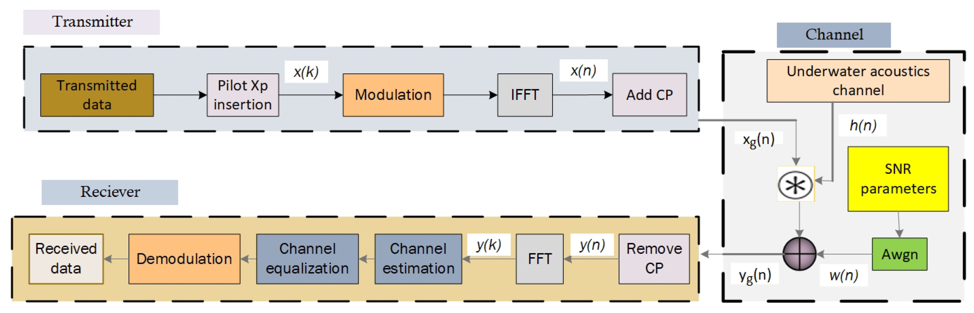
2.1. Conventional UWA OFDM Communication System

A schematic representation of the UWA OFDM system, as discussed in [36,37,38,39,40,41], is shown in Figure 1. The process begins with the generation of a binary data stream, to which pilot tones are added for the purpose of estimating the channel impulse response (CIR). This data is then modulated as shown in Figure 1. Following this, the inverse fast fourier transform (IFFT) is applied to shift the signal from the frequency domain to the time domain, utilizing N orthogonal narrowband subcarriers. The resulting time domain signal $x\left(n\right)$ is computed from the frequency domain symbols $X\left(k\right)$ as follows [23]:

$$x\left(n\right)=\mathrm{IFFT}\left\{X\left(k\right)\right\}={\displaystyle \frac{1}{N}}\sum _{k=0}^{N-1}X\left(k\right)e^{j2\pi {\displaystyle \frac{nk}{N}}},n=0,1,\dots ,N-1.$$

(1)

where:

• $X\left(k\right)$ is the frequency-domain representation of the OFDM symbol
• $x\left(n\right)$ is the time-domain signal obtained after IFFT,
• N is the total number of subcarriers,
• k is the subcarrier index, ranging from 0 to $N-1$,
• n is the time-domain sample index, ranging from 0 to $N-1$.

Figure 1. The conventional UWA OFDM communication system.

Figure 1. The conventional UWA OFDM communication system.

After the IFFT operation, a cyclic prefix (CP) is appended to the time domain signal to help counteract inter symbol interference (ISI) as depicted in Figure 1. The CP extended signal, $x_g\left(n\right)$, is defined as [23]:

$$x_g\left(n\right)=\left\{\begin{array}{cc}x(N+n),\hfill & \mathrm{for}n=-N_g,-N_g+1,\dots ,-1\hfill \\ x\left(n\right),\hfill & \mathrm{for}n=0,1,\dots ,N-1.\hfill \end{array}\right.$$

(2)

Here, $N_g$ indicates the number of samples in the CP. This step involves copying the last $N_g$ samples of $x\left(n\right)$ and placing them at the beginning of the symbol to form a guard interval. The resulting signal $x_g\left(n\right)$ has a total duration of $N+N_g$.

Once the signal propagates through the UWA channel, the received signal $y_g\left(n\right)$ is expressed as:

$$y_g\left(n\right)=x_g\left(n\right)\otimes h\left(n\right)+w\left(n\right),-N_g\le n\le N-1.$$

(3)

In this expression, ⊗ represents circular convolution, $h\left(n\right)$ denotes the CIR, and $w\left(n\right)$ is zero-mean Additive White Gaussian Noise (AWGN). The CIR can be modeled as:

$$h\left(n\right)=\sum _{i=0}^{r-1}{h}_i\delta (n-{\tau }_i),$$

(4)

where $\delta (·)$ is the Dirac delta function, r is the number of channel paths, and $h_i$, ${\tau }_i$ represents the complex gain and corresponding delay of the i-th path, respectively.

At the receiver side is in Figure 1, the cyclic prefix is removed, and the time-domain signal $y\left(n\right)$ is transformed back into the frequency domain using the Fast Fourier Transform (FFT) as follows:

$$Y\left(k\right)=\mathrm{FFT}\left\{y\left(n\right)\right\}={\displaystyle \frac{1}{N}}\sum _{n=0}^{N-1}y\left(n\right)e^{-j2\pi {\displaystyle \frac{nk}{N}}},k=0,1,\dots ,N-1.$$

(5)

Assuming ISI is effectively eliminated, the frequency-domain received signal can be modeled as [23]:

$$Y\left(k\right)=X\left(k\right)H\left(k\right)+W\left(k\right),k=0,1,\dots ,N-1,$$

(6)

where $H\left(k\right)$ and $W\left(k\right)$ are the Fourier transforms of the CIR $h\left(n\right)$ and noise $w\left(n\right)$, respectively. This equation establishes the relationship between the transmitted and received signals in the frequency domain over an UWA channel.

2.2. Deep Learning UWA OFDM Communication System Methods

Recent research shows that DNN-based methods for channel estimation can directly learn channel characteristics from received signals, outperforming traditional methods and simplifying system design by eliminating the need of channel estimation and equalization steps. During training, the received signal, containing both amplitude and phase information, serves as the input to the DNN, while the transmitted data are used as labels. The DNN learns to adjust its parameters by comparing predicted and actual transmitted data, allowing it to directly predict the transmitted data from the received signal without the need for explicit channel estimation, equalization, and demodulation as shown in Figure 2. Figure 3 clearly illustrates the difference between deep learning and TL. In TL, knowledge gained from one task can be transferred to a related task, thereby improving learning efficiency and performance. In contrast, traditional deep learning typically requires a separate learning process for each task, with its own dataset.

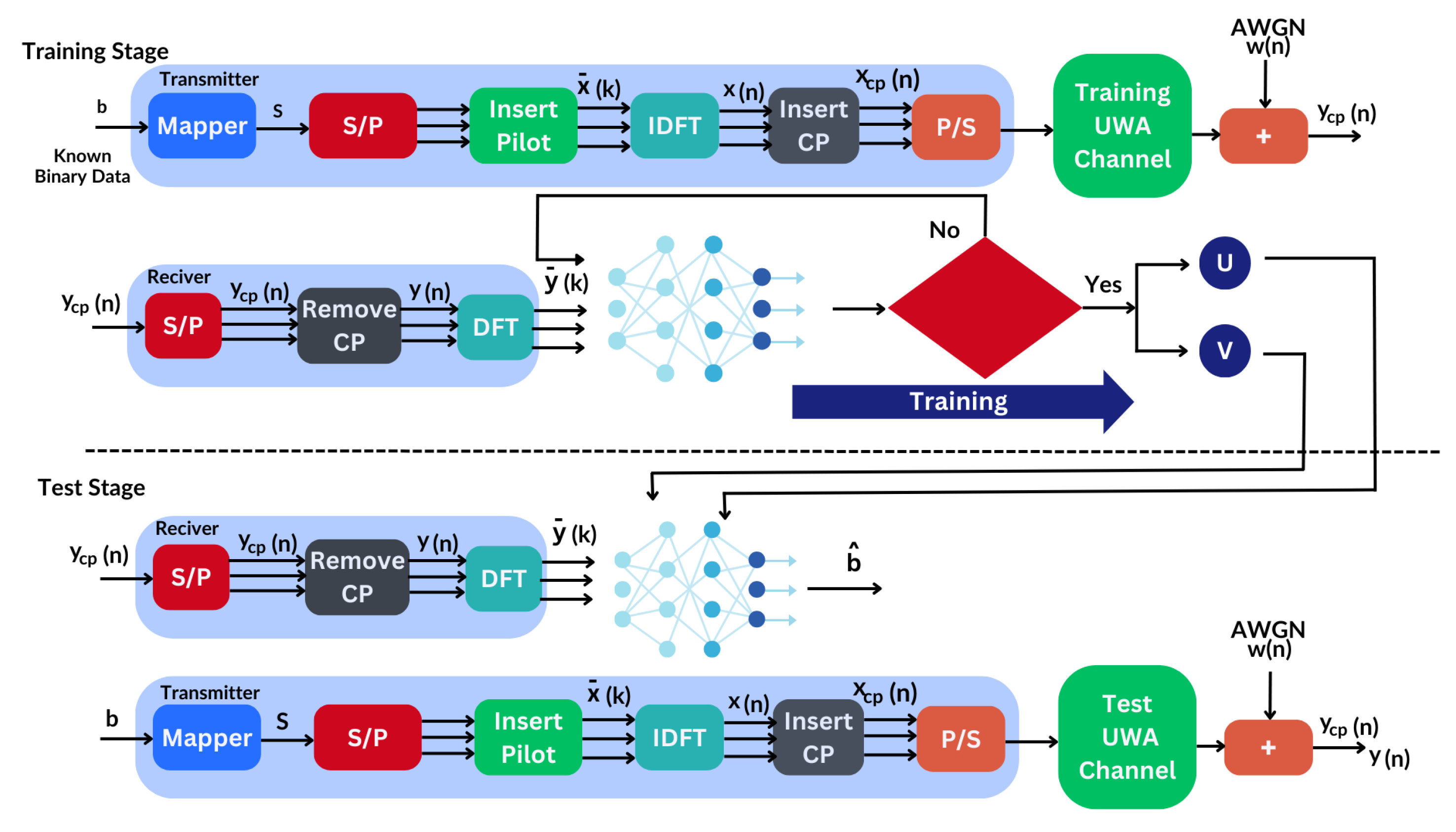
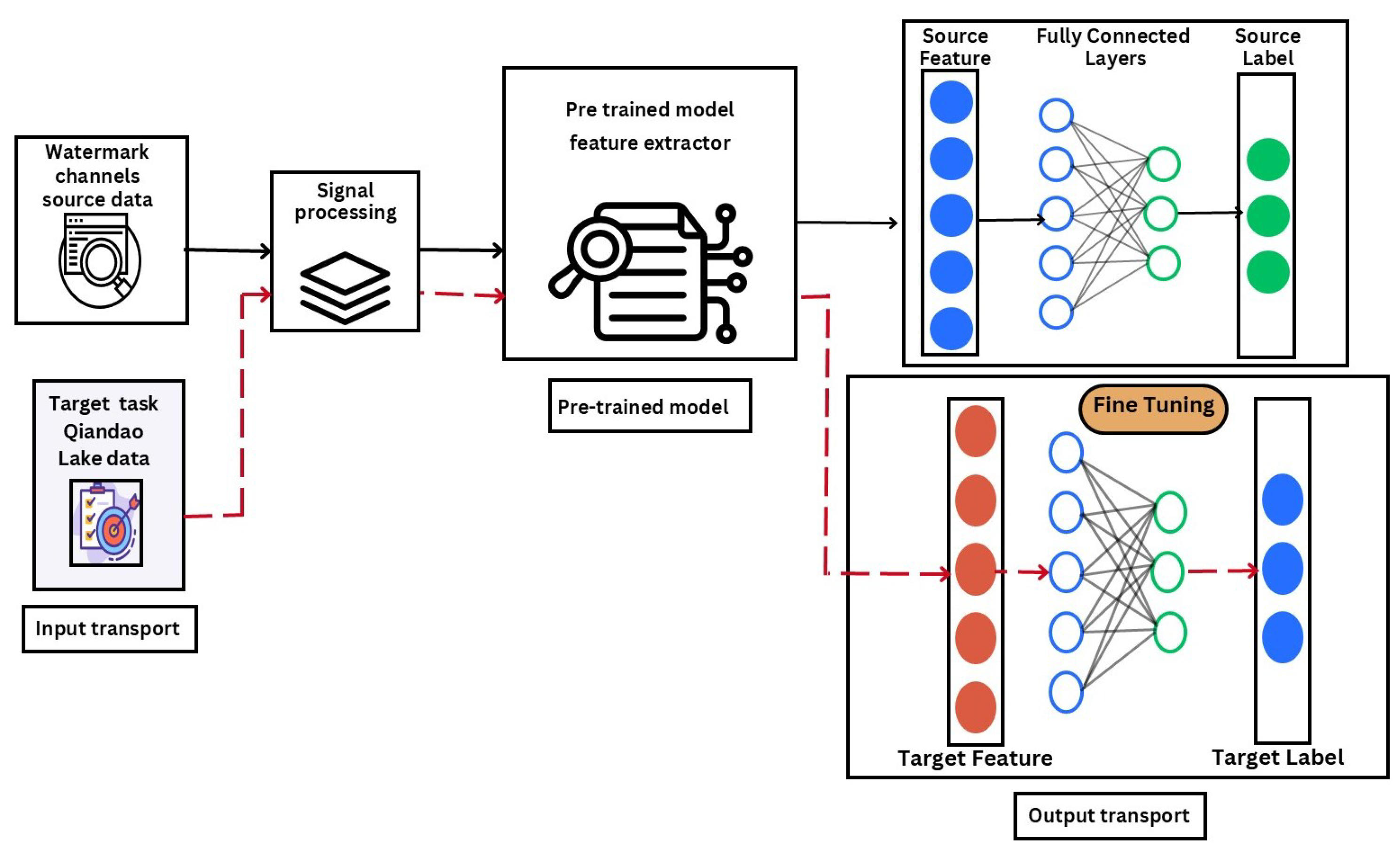
3. Proposed TL-Based UWA OFDM Receiver

The proposed TL-based UWA OFDM receiver utilizes a three-step transfer learning procedure to address the domain mismatch between the source (watermark channels) and target (Qingdao Lake) tasks. By pre-training a DNN model on the source task and fine-tuning it on the target task, the proposed approach significantly reduces the need for extensive training while maintaining high prediction accuracy.

3.1. Pre-Trained Model

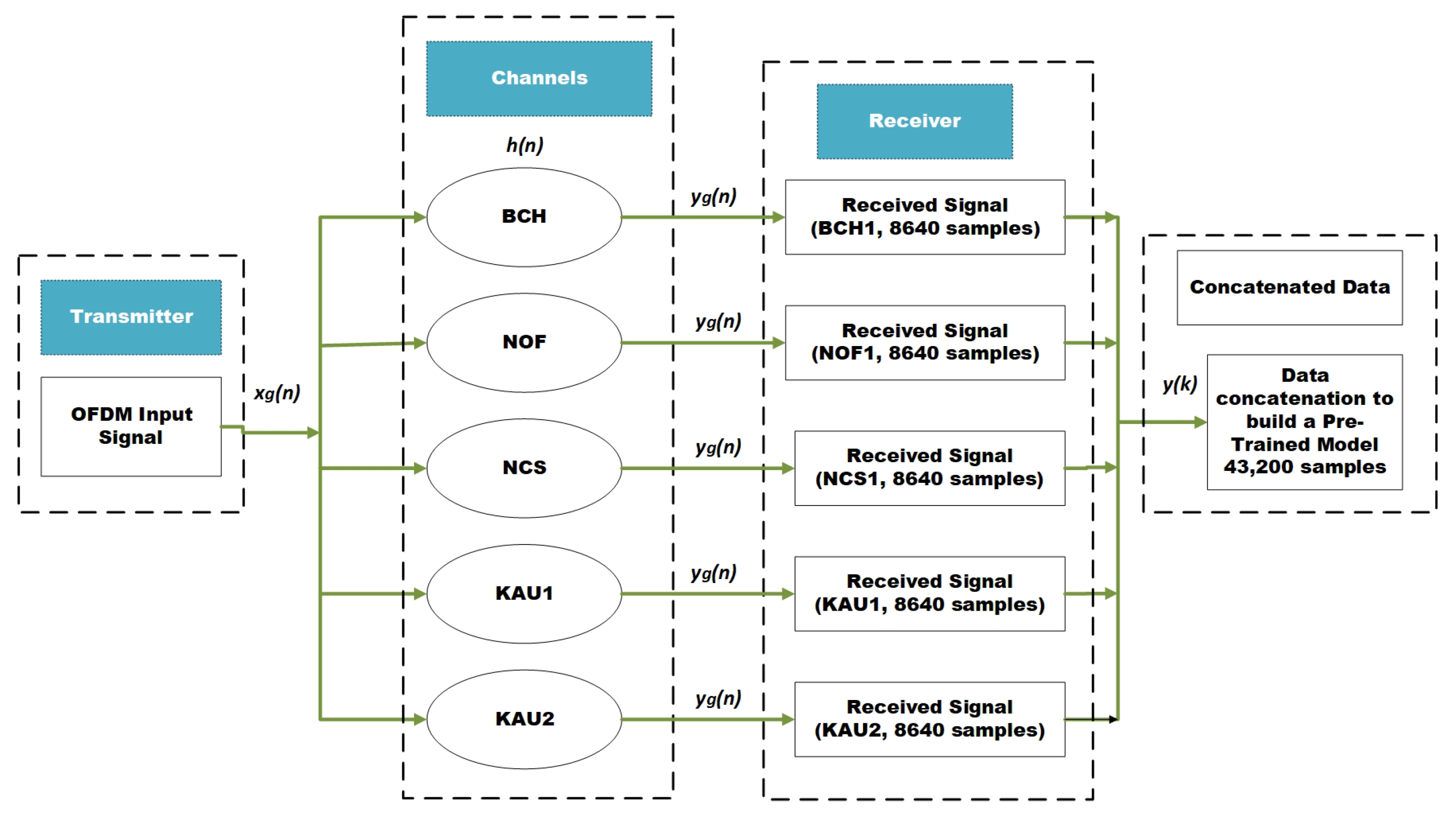
3.1.1. Data Collection and Training

The data collection and processing pipeline for pre-training a deep learning model in an underwater acoustic communication system is meticulously structured to ensure diversity and robustness. Figure 4 illustrates the OFDM communication. As the transmitted signal traverses the underwater channel, it undergoes complex propagation effects such as multipath fading, Doppler shifts, and attenuation, varying across different underwater conditions. Figure 4 showcases five distinct channel environments, BCH, NOF, NCS, KAU1 and KAU2. Figure 5 extends this concept by demonstrating how the received signal, rather than the transmitted signal, is used as the input feature for model training. Each channel (BCH, NOF, NCS, KAU1, and KAU2) introduces a distinct variation in the received signal due to different propagation conditions. The received signals from each environment are collected separately, forming variations in the dataset. Instead of training a model for each channel separately, the received signals are combined into one dataset, making it very diverse and complete. This data aggregation is necessary for pre-training a deep learning model with high generalization performance over different underwater conditions. For further assurance of dataset diversity, the received signal is collected across a range of SNR: −5 dB, 5 dB, and 15 dB. This is necessary so that for each SNR level, the received signal in each channel is recorded separately to make sure that the model sees different noise conditions and varying levels of signal degradation. Also, the data consists of more than 43,000 samples representing both the real and imaginary parts of the received signal. It leads to a comprehensive dataset that helps in training the model on all aspects of underwater conditions, improving the robustness and adaptability to unseen environments.

3.1.2. Pre-Trained Model Architecture

The pre-trained model extracts features from received signal data using a structured input of $[1,Nt\times 2,1]$, where $Nt=23$ represents the features in the received signal, consisting of real and imaginary components. Feature extraction is performed through convolutional layers: conv1 (kernel size $1\times 5$, 8 filters, stride 10) captures fundamental patterns, followed by conv2 (kernel size $1\times 5$, 16 filters), conv3 (kernel size $1\times 3$, 16 filters), conv4 (kernel size $1\times 3$, 32 filters), and conv5 (kernel size $1\times 3$, 32 filters), progressively refining features with smaller kernels and more filters. Each layer uses ReLU activation. Fully connected layers (fc1 to fc4) map extracted features to higher dimensions, with fc1 (64 units) using L2 regularization. fc2 and fc3 (32 units each) refine the learned representations, and fc4 outputs two class predictions. Batch normalization ensures stability, while dropout (rate 0.2) prevents overfitting. The softmax activation function transforms the logits into probabilities, enabling the model to effectively perform classification. The architecture of the pre-trained model is shown in

Table 1. Model Architecture of the pre-trained model.

Layer Type	Layer Name	Details
Input Layer	input	Input size: [1, Nt × 2, 1] where Nt = 46.
Convolutional Layer 1	conv1	Kernel: $1\times 5$, Filters: 8, Stride: 10.
Activation Layer	relu1.1	ReLU activation after conv1.
Convolutional Layer 2	conv2	Kernel: $1\times 5$, Filters: 16.
Activation Layer	relu2.1	ReLU activation after conv2.
Convolutional Layer 3	conv3	Kernel: $1\times 3$, Filters: 16.
Activation Layer	relu3.1	ReLU activation after conv3.
Convolutional Layer 4	conv4	Kernel: $1\times 3$, Filters: 32.
Activation Layer	relu4.1	ReLU activation after conv4.
Convolutional Layer 5	conv5	Kernel: $1\times 3$, Filters: 32.
Activation Layer	relu5.1	ReLU activation after conv5.
Fully Connected Layer 1	fc1	Units: 64, L2 regularization applied.
Batch Normalization Layer	bn1.1	Batch normalization for fc1.
Activation Layer	relu1.2	ReLU activation after fc1.
Dropout Layer	dropout1	Dropout rate: 0.2.
Fully Connected Layer 2	fc2	Units: 32, L2 regularization applied.
Batch Normalization Layer	bn2.1	Batch normalization for fc2.
Activation Layer	relu2.2	ReLU activation after fc2.
Dropout Layer	dropout2	Dropout rate: 0.2.
Fully Connected Layer 3	fc3	Units: 32, L2 regularization applied.
Activation Layer	relu3.2	ReLU activation after fc3.
Dropout Layer	dropout3	Dropout rate: 0.2.
Fully Connected Layer 4	fc4	Units: 2 (output classes).
Softmax Layer	softmax	Softmax activation for classification output.
Classification Layer	output	Categorical classification layer.

.

3.2. Transfer Learning and Fine-Tuning

The proposed TL approach is shown in Figure 6. During the fine-tuning phase of TL, the convolutional layers are frozen, retaining the weights learned during pre-training on the watermark channel datasets. These layers, having already captured general feature representations, remain unchanged while the fully connected layers are fine-tuned for the new classification task. These layers are fine-tuned on the target dataset ($D_T$) so that the model becomes specialized in recognizing features of the new task. The learning rate for the frozen convolutional layers is effectively constant, as their weights are not updated during the fine-tuning phase. This prevents the disruption of the feature-extraction process learned during pre-training. In contrast, the fully connected layers have an initial learning rate of ${\gamma }_2=0.01$. These layers are adapted to the new dataset while still utilizing the robust features extracted by the frozen convolutional layers. The learning rate for these layers decreases exponentially, following a piecewise schedule. This approach allows the model to adjust the fully connected layers for the new task while preserving the general feature representations captured by the frozen layers. This would allow for an optimal balance between the reuse and adaptation of features in the model so that it could generalize effectively on target data.

The process of model adaptation and fine-tuning is shown in

Table 2. Model training and fine-tuning.

Layer Type	Layer Names	Freezing Details
Convolutional Layers	conv1 to conv5	Weights and biases frozen during fine-tuning
Fully Connected Layers	fc1 to fc4	Trainable for adaptation to the target dataset

and

Table 3. Training Configuration Summary.

Training Type	Dataset Used	Max Epochs	Initial Learning Rate	Updated Layers	Frozen Layers
Pre-training	Watermark channel datasets ($D_s$)	20	${\gamma }_1=0.01$	All layers	None
Fine-tuning	Qingdao Lake dataset ($D_T$)	150	${\gamma }_2=0.01$	Fully connected layers	Conv. layers

. The methodology of the proposed TL-based Channel OFDM receiver is given in Algorithm 1.

Algorithm 1 Transfer Learning-based Channel OFDM receiver for UWA Communication

1: Input: 2:    $X_{train}$: Training data from watermark channels (BCH, NOF1, KAU1, KAU2, NCS1) 3:    $Y_{train}$: Corresponding transmitted bits for the training data 4:    $X_{test}$: Test data from Qingdao Lake channel 5:    $Y_{test}$: Corresponding transmitted bits for the test data 6:    ${\mathsf{\Theta }}_{pre}$: Pre-trained model weights from watermark channel data 7:    $\mathcal{L}$: Loss function (e.g., cross-entropy for classification) 8:    $E_{pre}$: Number of epochs for pre-training 9:    $E_{fine}$: Number of epochs for fine-tuning 10:    ${\eta }_{pre}$: Learning rate for pre-training 11:    ${\eta }_{fine}$: Learning rate for fine-tuning 12:    $\beta$: Regularization parameter 13:    P: Number of transmitted bits 14:    B: Number of batches 15: Step 1: Pre-training on watermark channels 16: for concatenation of the five watermark channels data (BCH, NOF1, KAU1, KAU2, NCS1) do 17:     Train a model $M_{pre}$ on $X_{train}$ with corresponding $Y_{train}$ 18:     Use Adam optimizer with learning rate ${\eta }_{pre}$ to minimize the loss function: $${\mathcal{L}}_{pre}={\displaystyle \frac{1}{P}}\sum _{i=1}^P{\left({\widehat{Y}}_i-Y_i\right)}^2$$ 19:     Store model weights ${\mathsf{\Theta }}_{pre}$ for use in fine-tuning 20: end for 21: Step 2: Fine-tuning on Qingdao Lake channel data 22: Initialize model $M_{fine}$ with pre-trained weights ${\mathsf{\Theta }}_{pre}$ 23: Freeze the convolutional layers of the pre-trained model 24: for epoch = 1 to $E_{fine}$ do 25:     for batch = 1 to B in $X_{test}$ do 26:         Forward pass: Calculate predicted transmitted bits ${\widehat{Y}}_{test}=M_{fine}\left(X_{test}\right)$ 27:         Compute binary cross-entropy loss for the test data: $${\mathcal{L}}_{fine}=-{\displaystyle \frac{1}{P}}\sum _{i=1}^P\left(Y_{test,i}log\left({\widehat{Y}}_{test,i}\right)+(1-Y_{test,i})log(1-{\widehat{Y}}_{test,i})\right)$$ 28:         Generate Data Using CIRs: Simulate the Qingdao Lake channel data using the CIRs to model the channel characteristics. 29:         Backward pass: Update weights for fully connected layers using Adam optimizer: $${\theta }_{i+1}={\theta }_i-{\eta }_{fine}\nabla {\mathcal{L}}_{fine}\left({\theta }_i\right)$$ 30:     end for 31: end for 32: Step 3: Evaluate model performance on test data 33: Compute final accuracy and loss on test data: $$Accuracy={\displaystyle \frac{\mathrm{Correct}\mathrm{predictions}}{\mathrm{Total}\mathrm{predictions}}}\times 100$$ 34: Compute Loss for the final model: $${\mathcal{L}}_{CE}=-{\displaystyle \frac{1}{P}}\sum _{i=1}^P\left(Y_{test,i}log\left({\widehat{Y}}_{test,i}\right)+(1-Y_{test,i})log(1-{\widehat{Y}}_{test,i})\right)$$ 35: Generate Confusion Matrix for predicted vs. true transmitted bits and calculate classification metrics: precision, recall, F1 score, and MCC. 36: Output: 37:    Fine-tuned model $M_{fine}$, performance metrics (accuracy, loss, confusion matrix) 38:    Final transmitted bit prediction results for Qingdao Lake channel data

• Dataset preparation: The dataset $D_T$ is split into training $D_{TTr}$ and testing $D_{TTe}$ sets.
• Freezing convolutional layers: The feature extraction layers, initialized with ${\mathsf{\Theta }}_{pre}$, remain fixed, while only the fully connected layers are updated.

The fine-tuning loss function is given by:

$$L_{fine}=-{\displaystyle \frac{1}{P}}\sum _{i=1}^P\left(Y_{test,i}log\left({\widehat{Y}}_{test,i}\right)+(1-Y_{test,i})log(1-{\widehat{Y}}_{test,i})\right),$$

(7)

where, P is the total number of test samples, $Y_{test,i}$ is the true label of the i-th test sample, where $Y_{test,i}\in 0,1$. ${\widehat{Y}}_{test,i}$ is the predicted probability that the i-th test sample belongs to class 1. The fine-tuning optimization follows:

$${\mathsf{\Theta }}_{fin}={\mathsf{\Theta }}_{fin}-{\gamma }_2\nabla L_{fine},$$

(8)

where, ${\mathsf{\Theta }}_{fin}$ is the parameters of the model (weights and biases) in the fine-tuning phase, specifically the fully connected layers. These parameters are adjusted during fine-tuning based on the gradient of the fine-tuning loss. ${\gamma }_2$ is the fine-tuning learning rate, which controls the magnitude of parameter updates during the fine-tuning process. $\nabla L_{fine}$ is the gradient of the fine-tuning loss function with respect to the model parameters.

4. Experimental Setup

This section begins with an introduction to the experimental setup, as detailed in Section 4.1, Section 4.2, Section 4.3 and Section 4.4. Following that, we delve into the configuration of the benchmark schemes in Section 4.5. Additionally, Section 4.6 outlines the performance evaluation metrics.

4.1. OFDM Setup

The OFDM setup for the UWA communication system is configured with critical parameters to optimize performance under challenging acoustic channel conditions as depicted in

Table 4. Overview of system parameters for UWA-OFDM.

Parameter	Value
UWA modulation scheme	OFDM
Sub-carriers, N	1024
Pilots	N/4
Pilot insertion	Comb
Guard interval	CP
CP size	N/4
Noise model	AWGN
SNR	−10:5:15 dB
Sampling frequency $f_s$	48–96 kHz
Carrier frequency	14 kHz
Frequency spacing	4.88 Hz
OFDM symbol period	0.204 s
Modulation scheme	BPSK
UWA channel	Watermark

. The system employs OFDM modulation, leveraging 1024 sub-carriers. Comb-type pilot insertion with an N/4 spacing facilitates accurate channel estimation and synchronization, crucial for maintaining transmission integrity in dynamic environments. A CP is used as a guard interval to mitigate ISI caused by multipath propagation, typical in underwater environments. The system operates at a sampling frequency in the range of 48 kHz to 96 kHz, depending on the specific configuration. A 14 kHz carrier frequency is usually used in UWA while the system is modeled under AWGN with an SNR range of −10 dB to 15 dB, representative of typical underwater noise environments. BPSK modulation is employed for its robustness under low SNR conditions, ensuring reliable communication.

4.2. Channel Setup

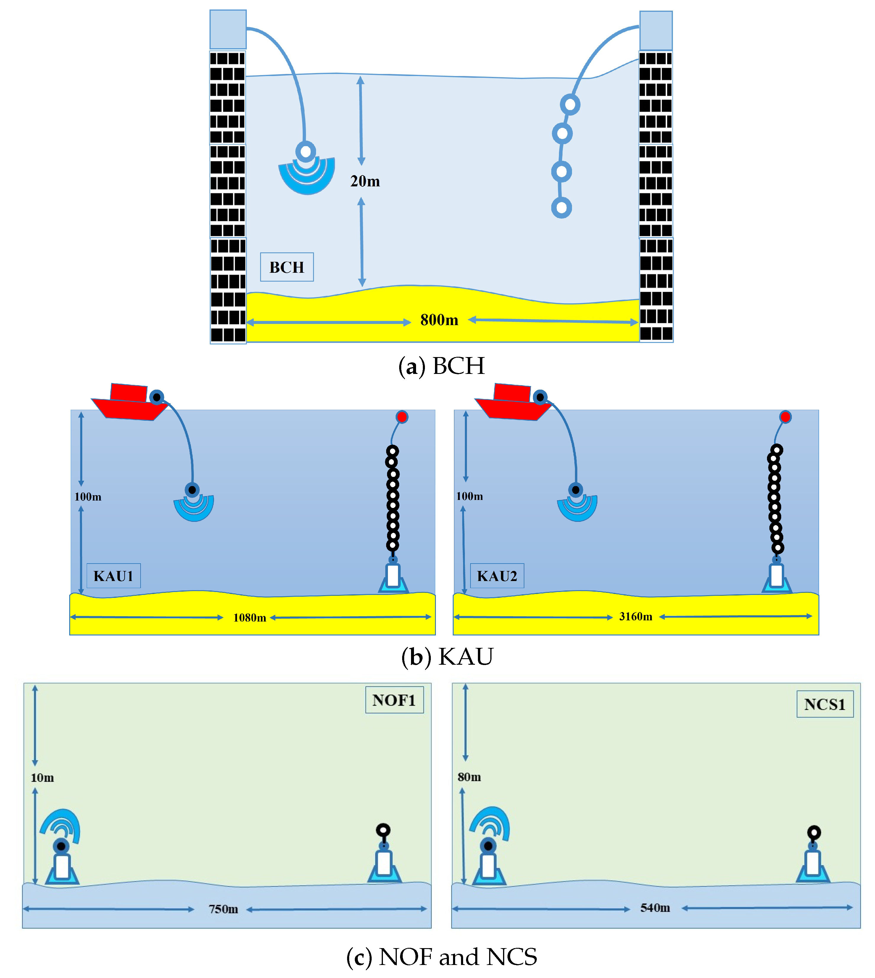
4.2.1. Watermark Channel Setup

The watermark channel [42] setup encompasses a series of experiments conducted in diverse underwater environments, each selected to test the system’s resilience to varying propagation conditions. The test locations span fjords, harbors, and shelves, with operational ranges from 540 m to over 3000 m and water depths ranging from 10 m to 80 m as given in

Table 5. The experimentation setup of different watermark channels.

Name	NOF1	BCH	KAU1	KAU2	NCS1
Environment	Fjord	Harbour	Shelf	Shelf	Shelf
Time of year	June	June	July	July	June
Range	750 m	800 m	1080 m	3160 m	540 m
Water depth	10 m	20 m	100 m	100 m	80 m
Transmitter depl.	Bottom	Suspended	Towed	Towed	Bottom
Receiver depl.	Bottom	Suspended	Suspended	Suspended	Bottom
Frequency range	10–18 kHz	32.5–37.5 kHz	4–8 kHz	4–8 kHz	10–18 kHz
Sounding duration	32.9 s	59.4 s	32.9 s	32.9 s	32.9 s
Delay coverage	128 ms	102 ms	128 ms	128 ms	32 ms
Doppler coverage	7.8 Hz	9.8 Hz	7.8 Hz	7.8 Hz	31.4 Hz
Type	SISO	SIMO	SIMO	SIMO	SISO
Element spacing	-	1 m	3.75 m	3.75 m	-
Cycles	60	1	1	1	-
Total play time	33 min	1 min	33 s	33 s	33 min

. The transmitter is positioned in different configurations, from bottom-mounted to suspended, influencing the multipath propagation characteristics and the receiver’s signal quality.

The frequency range varies from 4 kHz to 37.5 kHz, allowing comprehensive testing across different acoustic spectra. Sounding durations range from 32.9 s to 59.4 s, ensuring robust data collection over extended periods. The system accommodates delay spreads of up to 128 ms and Doppler shifts up to 9.8 Hz, crucial for maintaining signal integrity under motion-induced frequency variations. SISO and SIMO receiver configurations are tested, with element spacings ranging from 1 m to 3.75 m, enhancing spatial diversity for improved reception. Total experiment durations vary, with some lasting up to 33 min, enabling a thorough assessment of the system’s performance across diverse real-world conditions. The configuration of Watermark channels are shown in Figure 7a–c.

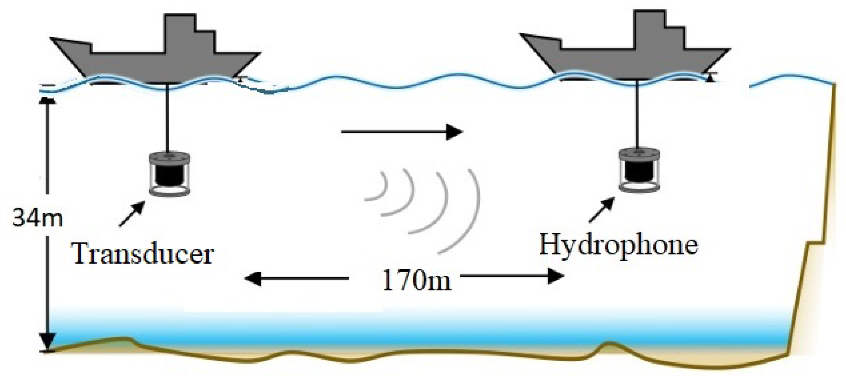
4.2.2. Target Channel Setup

To better understand the time-varying characteristics of the UWA channel and their impact on network performance, a comprehensive experiment was carried out on Qingdao Lake, Hangzhou, Zhejiang Province. The experiment aimed to collect real-world data for testing the TL-based OFDM receiver model proposed. The environmental conditions in the lake were carefully monitored through the deployment of several sensors, which provided a rich dataset of critical environmental parameters, including water temperature, salinity, pressure, and wind speed at different times of the day (morning, noon, and evening), as shown in

Table 6. Environmental Measurements in Qingdao Lake.

Parameter	Morning	Noon	Evening
Water Temperature (°C)	9.2	12.5	10.1
Salinity (ppt)	0.12	0.14	0.13
Pressure (Pa)	32.5	32.2	32.9
Wind Speed (m/s)	3.1	4.2	3.8

.

Figure 8 depicts the setup for the lake experiment. The measurement has lasted six days, and channel measurements are taken over the selected intervals to capture the variability in the underwater communication. These data gathered include all key parameters that characterise the underwater channel: distance between transmitter and receiver, depth, sound speed profile, and the measured SNR. Other important underwater communication factors, such as multipath spread and Doppler spread, were measured. Maximum multipath delay spread was 27.5 ms and the Root Mean Square (RMS) multipath delay spread was 29.3 ms. These values give the magnitude of the reflected signal from various underwater surfaces, the water surface and lakebed along with its delay. The Doppler spread, which gives a measure of the frequency shift due to the relative motion of the transmitter and receiver with respect to the environment, was also quantified. The maximum Doppler spread was 2.3396 Hz, while the RMS Doppler spread was 3.1487 Hz, showing moderate motion-induced variations.

The data acquired in this experiment are used for testing the proposed TL model. The pre-trained model, here trained using a diverse set of underwater channels, would be fine-tuned with real-world data from Qingdao Lake. It is crucial for the TL model to be capable of adapting to the Qingdao Lake environment. Fine-tuning the pre-trained model with real channel data will enable it to handle the dynamic changes of the underwater channel and improve performance under real conditions. This experimental setup and data collection process provide practical validation of the transfer learning-based OFDM receiver and make sure that the model will be able to handle the complexities of other real underwater channels. Measured parameters of the Qingdao Lake channel are given in

Table 7. Measured parameters and environmental variability of Qingdao Lake channel.

Parameter	Value/Observation	Unit/Description
Distance (Range)	170	meters (m)
Transmitter Depth	34	meters (m)
Receiver Depth	34	meters (m)
Sound Speed Profile (SSP)	1480–1495	m/s (dependent on depth)
Maximum Multipath Spread (${\tau }_{max}$)	0.0275	seconds (s)
RMS Multipath Spread (${\tau }_{rms}$)	0.0293	seconds (s)
Maximum Doppler Spread ($v_{max}$)	2.3396	Hz
RMS Doppler Spread ($v_{rms}$)	3.1487	Hz
Environmental Temperature Range	9–12	°C
Salinity	Low (Freshwater)	Qingdao Lake is a freshwater lake
Probe Signal Type	LFM	Frequency: 8000–16,000 Hz
Number of Sounding Signals per Group	272	Each group lasts 30 s
Testing Frequency	3 times per day	Interval ≈ 3 min between groups
Number of Data Samples Collected	34	Effective measured channel

and the configuration is given in Figure 8. In addition, the CIRs and time-varying impusle response (TVIRs) of different channels used in the simulations are given in Figure 9 and Figure 10, respectively.

The channel characteristics in Figure 11 clearly illustrate that the UWA channels are time-varying in nature due to the dynamic and harsh environmental characteristics. The time series evolution of the signal received shows time-varying signal strength. In Figure 11a,b, the signal remains almost stable with a gradual fading behavior, which is normal in underwater environments. This attenuation, most probably due to multipath propagation, depends on reflections from surfaces such as the water surface or lakebed, causing delays in the received signal. With time, different color variations in the plots reflect changes in signal strength, indicative of environmental conditions such as water currents that alter the propagation of sound waves. Delay Doppler spread plots give a clearer view of the distribution of the signal frequency and time delay. From Figure 11a,b, the energy is concentrated at low Doppler shifts and short time delays, indicating dominance of the direct path. However, for Figure 11c, we see significant Doppler shifts, indicating there is a relative motion between transmitter and receiver. This introduces frequency shifts characteristic of underwater communication, where water movements or objects take their toll on signal frequency. Instead, the delay Doppler spread becomes more sophisticated, with the energy spread around a wider area of frequencies and time delays in Figure 11e, indicating larger object movements and/or increased water turbulence. The power delay profile plots give the distribution of the signal’s energy over the time delays. Figure 11a–c have a dominant peak due to the direct path, but with smaller peaks indicating some multipath components, meaning reflections are present though the direct path is primary. Accordingly, the profiles represented by Figure 11e,f depict higher complexity and multi-peaks due to strong multipath propagation, hence proving high reflections on multiple surfaces of various distances.

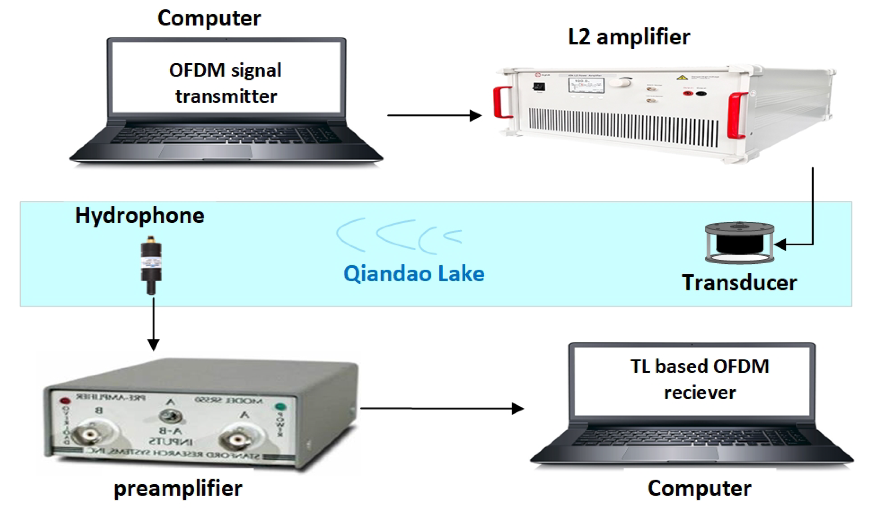
4.3. Hardware Implementation of Proposed Scheme

Experimental setup was conducted in Zhejiang Province, China, in Qingdao Lake to test the robustness and generalization capability of the proposed TL-based receiver. The entire hardware setup is depicted in Figure 12. On the transmitter side, a power amplifier is used that is a Class L2 power amplifier. Prior to being fed to the Class L2 power amplifier, a computer running MATLAB R2023a is used to generate OFDM signal. The amplified electrical signal is then fed to an UWA transducer. On the receiving side, the acoustic signals are received by a hydrophone and the received acoustic waves are converted back into electrical signals. The analog signals are then supplied to a low-noise preamplifier that carries out signal amplification as well as signal conditioning. The amplified signals are converted into digital form and are received by the receiver-side computer that executes the TL-based OFDM training and prediction.

4.4. Proposed Model Training Setup

The proposed model training setup follows a well-structured approach to TL in UWA communication. Training includes pre-training and fine-tuning of the model; during pre-training, the training features from each channel are concatenated. Afterwards, 80% is for training and 20% for validation in order for the model to learn the feature extraction effectively. Then, 50% of the Qingdao Lake dataset was used for fine-tuning, further divided into 80% for training and 20% for validation. This can be visualized in

Table 8. Training and validation data preparation.

Step	Details
Datasets Used	Watermark channels data for pre-training
Label Data	Concatenated categorical labels from the corresponding datasets
Data Concatenation	Training features of each watermark channel are concatenated
Training/Validation Split	80% training, 20% validation
Fine-tuning Data	50% of data Qingdao data used for fine-tuning, split further into 80% training and 20% validation
Testing Data	Remaining 50% of input data Qingdao Lake data used exclusively for testing

. In this process, convolutional layers are frozen; only fully connected layers are updated to allow the model to adapt exclusively to the new dataset while retaining general features learned during pre-training. At last, a testing phase using the remaining 50% of the Qingdao Lake dataset, kept exclusively for model performance evaluation, is performed. The validation metrics used are accuracy, precision, recall, F1-score, and a confusion matrix.

4.5. Benchmark Methods

The benchmark models LS [9,10,11,12,13,14,15,16,17,18,19], MMSE [20,21], and DNN [26,27,28,29,30,31,32,33,34] estimators offer different approaches to UWA channel estimation, each with its own strengths and limitations. These state-of-the-art methods are used as benchmark schemes for comparison, which are explained and analyzed in the following subsections.

4.5.1. Least Square

The LS algorithm is often used for channel estimation. This method aims to minimize the square of the error between received pilots and transmitted pilots.

4.5.2. MMSE Estimator

The MMSE estimation is proposed as a solution to the noise-prone flaws of LS estimation. This method aims to reduce the MSE between the actual channel and its estimation. However, obtaining the auto-correlation function of the channel and the noise variance, which is necessary for this task, can be challenging in an underwater environment. It can also be computationally expensive, making it inappropriate for real-time implementation in underwater communication systems; however, it provides enhanced performance compared to LS estimation.

4.5.3. FC-NN

The deep learning methods used in UWA channel estimation are based on the backpropagation neural network [29]. It capture complex nonlinear relationships by mapping the CIR with received signal and the transmitted pilots. The FC-NN used in this paper comprises five dense layers. This configuration allows the NN to effectively learn and represent the underlying mapping between input features and the CIR in the UWA channel.

4.5.4. OMP

OMP is a channel-estimation algorithm in UWA due to its effectiveness in taking advantage of channel sparsity. UWA channels tend to possess a small number of strong multipath components, and sparse recovery methods like OMP are thus most appropriate. This approach offers higher quality estimation with less pilot overhead compared to traditional approaches like LS and is an appropriate baseline against which sparse channel-estimation performance can be measured.

Traditional methods like LS suffer from high noise sensitivity and poor performance at low SNR due to the inability to exploit channel statistics. In contrast, MMSE improves accuracy through channel and noise statistics but at the cost of high computational complexity and perfect channel knowledge, which is difficult to obtain in dynamically changing underwater environments. Recently, neural networks including fully connected models, have performed more effectively by learning nonlinear channel behavior and even end-to-end OFDM receivers combining estimation, equalization, and demodulation. However, underwater channels create model mismatch, requiring ongoing retraining that prevents practical deployment. In addition, OMP, relying on channel sparsity, fails due to the diffuse multipath and Doppler effects prevalent underwater and is also computationally intensive. Therefore, the proposed TL-based OFDM receiver is presented as a solution, which enables models to efficiently learn to accommodate changing channel conditions at a minimal level of retraining. This approach addresses the channel mismatch issue and achieves improved robustness under dynamic underwater environments.

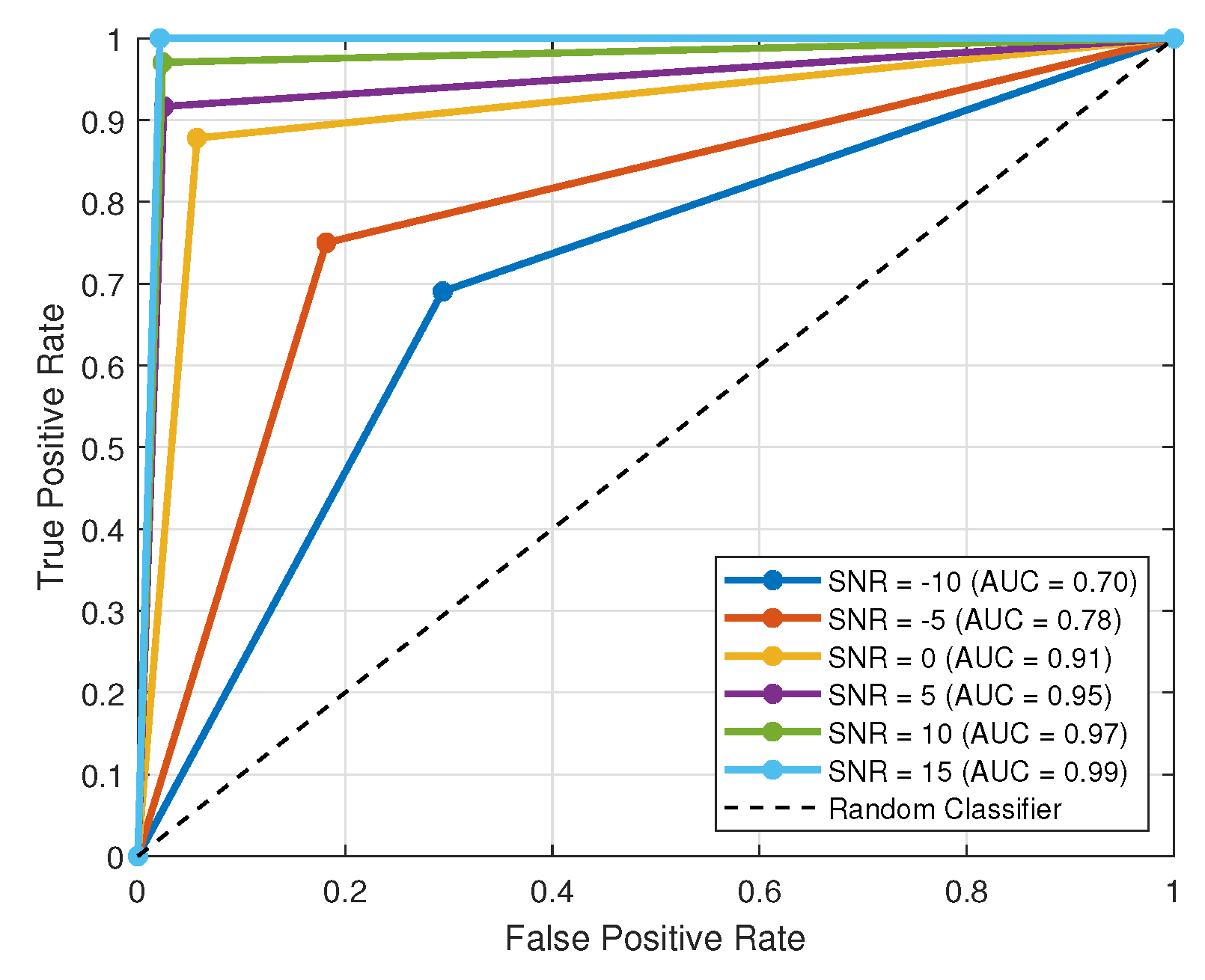
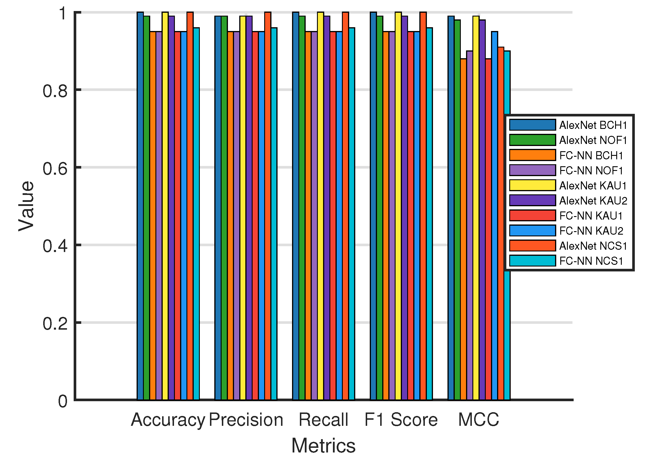
4.6. Performance Validation Metrics

The evaluation of deep learning-based OFDM receivers for UWA communication includes several key performance metrics [43]. BER measures the accuracy of data transmission by comparing the number of bit errors to the total number of bits sent [44]. Lower BER values indicate better transmission accuracy. In addition, accuracy is the proportion of correctly predicted bits. Higher accuracy values reflect better receiver performance [45]. In addition, Precision, recall, and F1 score are used to evaluate classification performance. These metrics assess model detection accuracy and classification balance [46,47,48]. Moreover, the Mathews correlation coefficient (MCC) evaluates binary classification performance. It takes into account true and false positives and negatives and gives a balanced score even if the classes are of different sizes, making it a reliable metric for performance evaluation. Higher MCC indicates better model accuracy [49,50]. Also, the confusion matrix summarizes classification performance, showing true and false classifications across classes. The BER vs. SNR curve is used to assess receiver performance under varying noise levels. It helps identify performance thresholds for optimization in underwater conditions.

5. Simulation and Experimental Results

In this section, we present a comprehensive analysis of the experimental results. Section 5.1 focuses on the Average Fade Rating (AFR) analysis of watermark channels and its impact on the OFDM receiver’s performance. Section 5.2 explores the receiver’s behavior when trained and tested on the same channel (where each channel is split into training and testing sets). Section 5.3 evaluates the model’s robustness in challenging UWA environments, addressing environmental mismatches. Section 5.4 investigates the effectiveness of pre-trained models, emphasizing their ability to generalize across diverse scenarios. Section 5.5 delves into the performance of transfer learning models, testing adaptability to real-world data from Qingdao Lake. Finally, computational complexity is analyzed in Section 5.6.

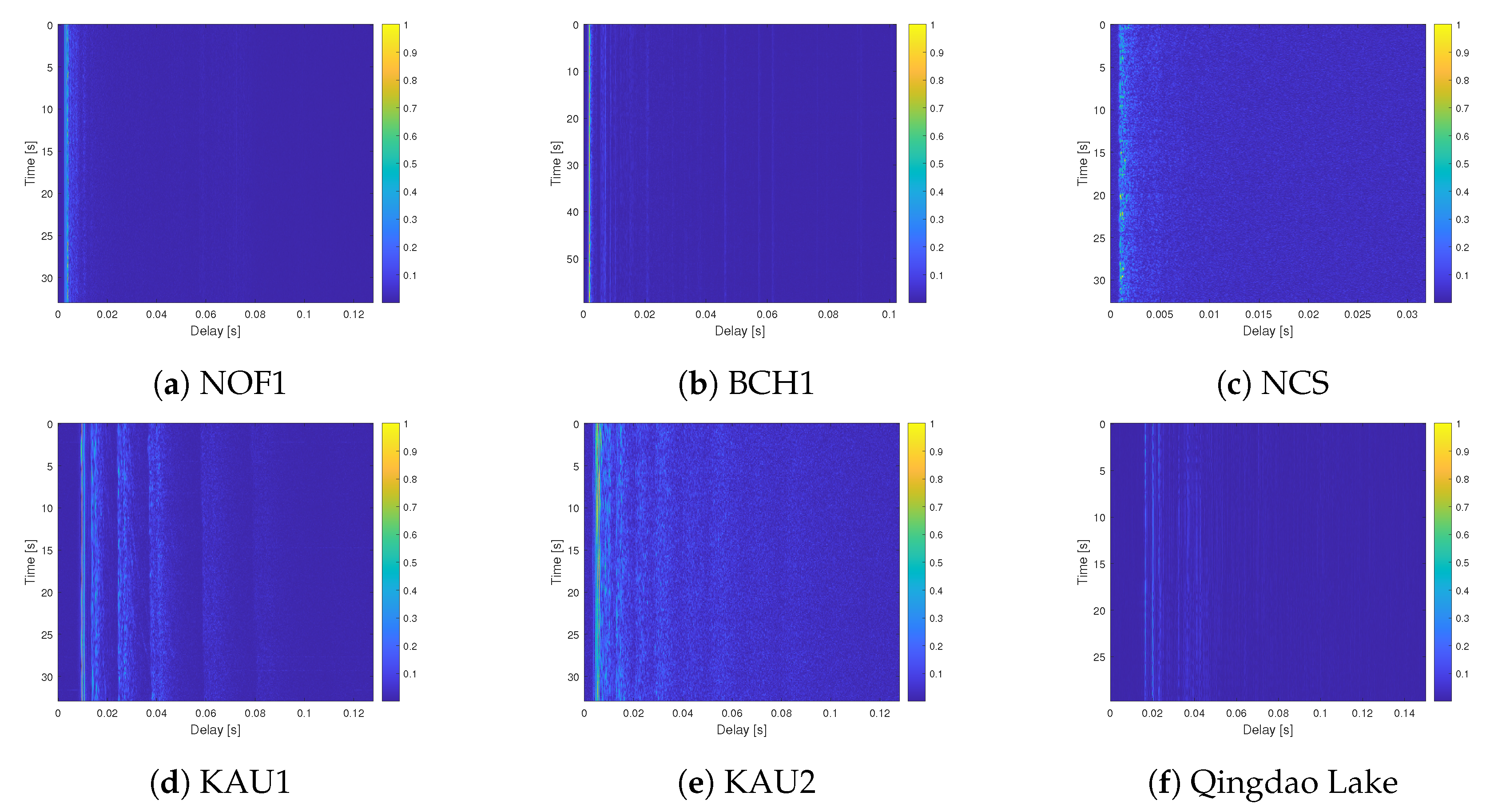
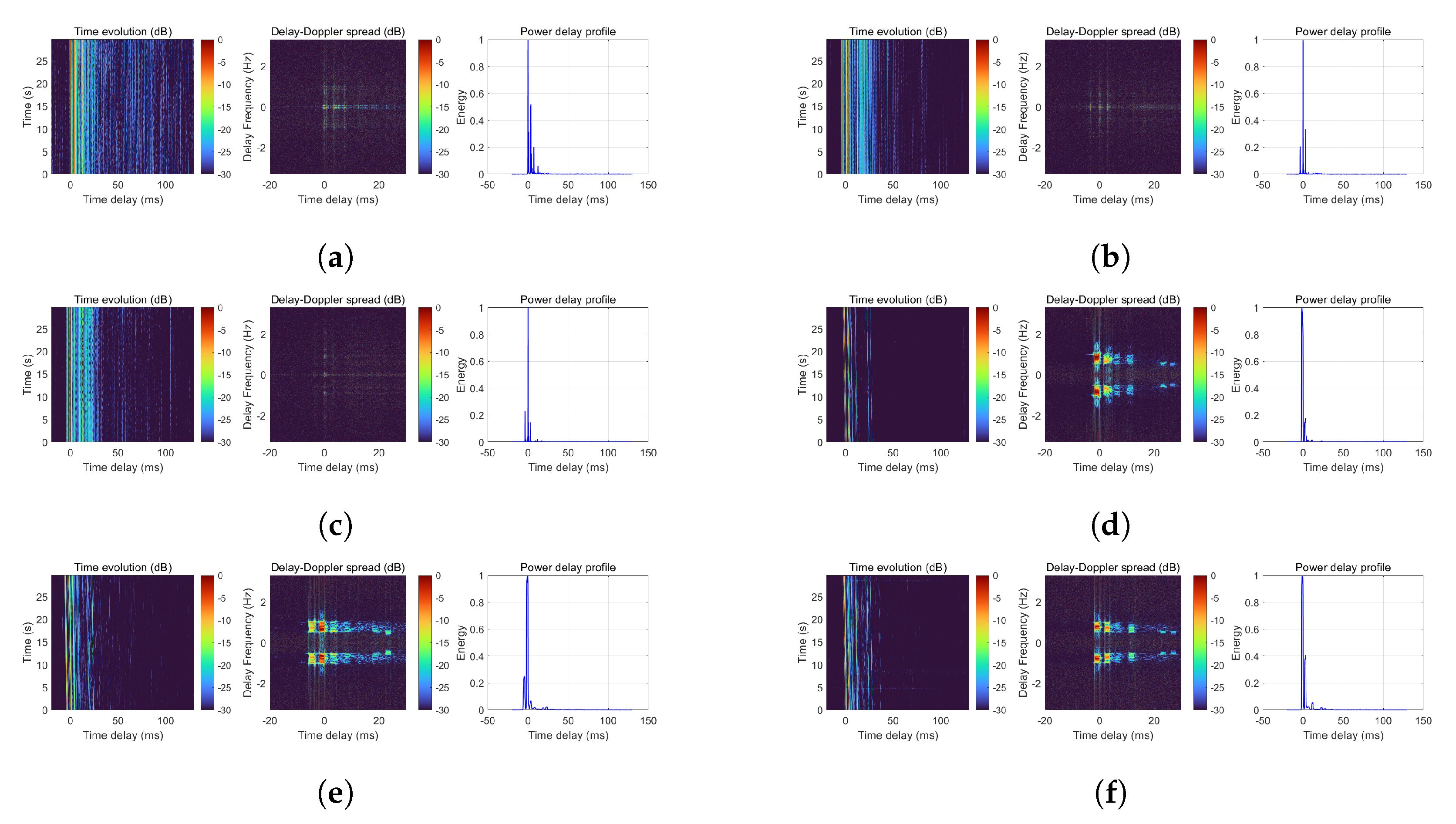
5.1. Average Fade Rating Analysis of Watermark Channels and Impact on OFDM Receiver

It is imperative to conduct an analysis of the various channels. This will not only enhance the understanding of UWA channels, but also facilitate a systematic evaluation of channel-estimation performance. In [51], a detailed analysis is presented on the challenges associated with watermark channels. An illustration of how Empirical Mode Decomposition (EMD) filtering is applied to BCH, NOF, NCS, and KAU channels can be seen in

Table 9. AFR of WATERMARK channels, calculated by using EMD [51].

Channels	P(d)	P(r)	P(h)	AFR
KAU	0.0011	0.0063	0.0074	0.8521
BCH1	0.0016	0.0010	0.0026	0.3868
NOF1	0.0018	0.0006	0.0024	0.2581
NCS1	0.0002	0.0043	0.0045	0.9636

. EMD filtering is pivotal in this research as it has allowed scholars to design a way to evaluate individual UWA channels by determining the average fade rate, a metric that is exhibited in Table 9.

EMD possesses the unique capability to separate a signal into a trend signal and a random signal. When considering the UWA channel, it’s conceived as a blend of both slow and fast fading. This is evident when each tap of the channel is denoted as $h_i\left(n\right)=d_i\left(n\right)+r_i\left(n\right)$. Here, $d_i\left(n\right)$ epitomizes the deterministic or what can be referred to as the “trend” segment of the channel, whereas $r_i\left(n\right)$ denotes its random component. Intriguingly, this deterministic portion is labeled “pseudo-deterministic” [51]. Further diving into the mechanics, each channel tap, represented as $h_i\left(n\right)$, can undergo decomposition via EMD. To isolate the trend from the purely random process, each channel tap can be represented in the empirical mode space in [51] as:

$$h_i\left(n\right)=\underset{r_i\left(n\right)}{\underbrace{\sum _{q=1}^{S_i}{m}_{i,q}\left(n\right)}}+\underset{d_i\left(n\right)}{\underbrace{\sum _{q=S_i+1}^{Q_i}{m}_{i,q}\left(n\right)+e_i\left(n\right)}},$$

(9)

where $m_{i,q}\left(n\right)$ represents the q-th mode out of the total $Q_i$ modes, and $e_i\left(n\right)$ is the decomposition residue. The parameter $S_i$ denotes the decomposition order, which separates the two components. A pivotal metric called the Average Fade Rate (AFR) emerges from this, offering a glimpse into the quality of the channel. This rate is ascertained from the potency of the random segment $r_i\left(n\right)$ in relation to the channel $h_i\left(n\right)$. The AFR in [51] is defined as:

$$AF{R}_R=10log\left({\displaystyle \frac{P_{ow}\left(r\right)}{P_{ow}\left(h\right)}}\right)=10log\left({\displaystyle \frac{{\sum }_{n=1}^N{\sum }_{i=1}^I\left|\right|r_i\left(n\right){\left|\right|}^2}{{\sum }_{n=1}^N{\sum }_{i=1}^I\left|\right|h_i\left(n\right){\left|\right|}^2}}\right),$$

(10)

where:

• $P_{ow}\left(r\right)$ is the power of the random component $r_i\left(n\right)$.
• $P_{ow}\left(h\right)$ is the power of the total channel $h_i\left(n\right)$.
• $P_{ow}\left(d\right)$ is the power deterministic or trend component $d_i\left(n\right)$. Since the channel tap $h_i\left(n\right)$ is modeled as the sum of the trend component $d_i\left(n\right)$ and the random component $r_i\left(n\right)$, the total power of the channel tap can be approximately decomposed as: $P_{ow}\left(h\right)$ ≈ $P_{ow}\left(d\right)$ + $P_{ow}\left(r\right)$.
• N is the total number of samples.
• I is the number of channel taps.

This analysis indicates that the NOF and BCH channels exhibit relatively high quality, as their stable paths concentrate most of the received signal energy. In contrast, the NCS and KAU channels, characterized by high AFR values, present greater challenges due to numerous distinct trailing paths and fluctuating arrival patterns. The experimental results are discussed in detail in the following subsections. In addition, to verify the representativeness of the measured WATERMARK channels, we performed an error analysis by comparing the experimental channel’s AFR (Qingdao Lake) with the measured WATERMARK channels’ AFR. The AFR of the experiment channel, as obtained from the Qingdao Lake experiment, is 0.25. Table 9 shows the values of the AFR of the observed channels. The results show that experimental channel is close to the NOF1 and BCH1 channels. On the contrary, the experimental channel AFR is far from the NCS and KAU channel whose AFR values are quite higher and absolute errors greater. As Table 9 shows, NOF and BCH are quite good quality channels where the majority of the arriving energy is carried by stable and dominant propagation paths. NCS and KAU are poor channels with unstable signals. These findings show that the experimental channel has similar fading characteristics to what is observed in more stable underwater scenarios of the NOF and BCH channels, thereby confirming and affirming the validity of the measured data set in modeling real time situations.

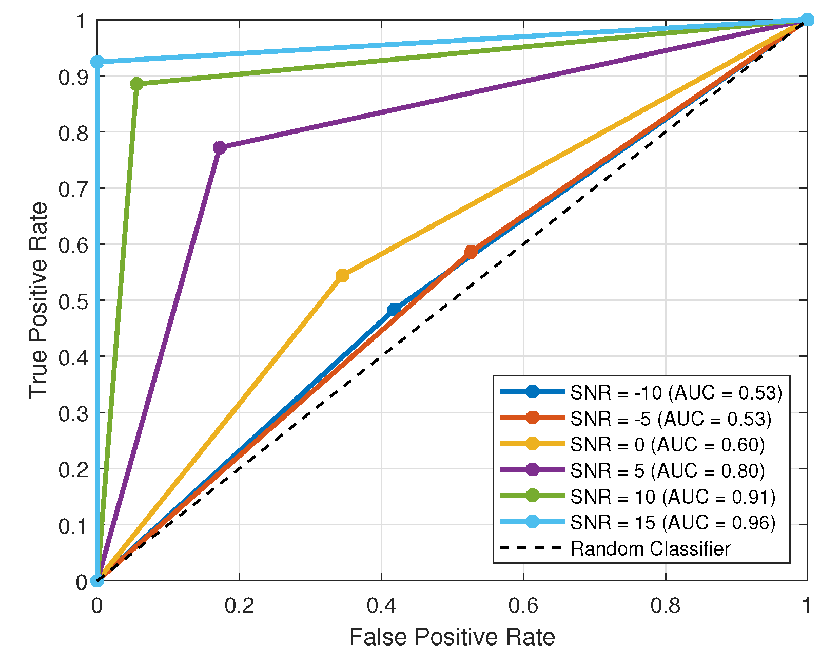
5.2. Deep Learning-Based OFDM Receiver, When Trained and Tested on the Same Channel (Where Each Channel Is Split into Training and Testing Sets)

This section presents an evaluation of the performance gains achieved by the proposed model within an OFDM system. A series of experiments are conducted to compare our approach with various OFDM receiver schemes for UWA communication, including both traditional methods and FC-DNN based models. Figures 13–20 offer a detailed performance comparison of the different techniques including LS, OMP, MMSE, FC-NN, and DNN in the context of UWA communication. Figure 13, which compares the training and validation accuracy and loss of DNN and FC-NN, highlights the superior performance of DNN across all channels. DNN consistently achieves higher accuracy and lower loss, particularly in complex channels like KAU1 in Figure 13b, where its validation accuracy remains around 85–90%, compared to FC-NN’s 75–80%. This is attributed to DNN’s ability to capture complex patterns and spatial dependencies in the data, making it robust to noise and channel variations. In contrast, FC-NN’s simpler architecture struggles to model non-linear relationships, leading to higher loss and lower accuracy, especially in challenging environments. While FC-NN is faster to train and computationally less demanding, its inability to generalize well in complex channels limits its practical applicability.

Figure 14 and Figure 15 show the confusion matrices of the FC-NN and DNN when SNR = 15 dB. The FC-NN has more misclassifications, particularly in two complex channels, such as KAU1 and KAU2, where it misclassifies 12 instances in BCH1. This is because the FC-NN has failed to learn complex pattern and nonlinear relationship in high AFR channels. On the contrary, the DNN is quite robust; it only misclassifies a few instances in all channels. For instance, in BCH1, the DNN makes only four misclassifications, showing that it works efficiently on complex and time-varying channels. This is because the DNN can extract hierarchical features and model spatial dependencies, thereby performing impressively well in both stable and challenging environments. While the DNN requires higher computational powers, it performs better in different scenarios and, therefore, will be more appropriate for underwater communication systems.

Figure 16 and Figure 17 present the ROC curves of the DNN for UWA channels (NOF1 and BCH1) across various SNRs. These curves illustrate the model’s classification performance, with AUC values reflecting its overall effectiveness. In the NOF1 channel Figure 16, the DNN achieves robust performance, with an AUC approaching 1 at higher SNRs, signifying strong classification capability even in noisy environments. The model’s ability to maintain high TPR and low FPR at SNRs as low as 5 dB indicates its resilience in stable, low-fade conditions. For the BCH1 channel in Figure 17, performance is more sensitive to noise. The AUC increases significantly with SNR, highlighting the DNN’s reliance on cleaner signals for accurate classification. At low SNRs, the model struggles, but at higher SNRs, it effectively adapts to the channel’s inherent fluctuations.

Figure 18 reveals that the DNN consistently outperforms the FCNN in key performance metrics, including accuracy, precision, and MCC, across all channels. Specifically, at 15 dB SNR, the DNN achieves near perfect scores in these metrics, showing a substantial advantage over the FCNN, which has slightly lower performance, especially in more complex channels like KAU1 and KAU2. This solidifies the DNN’s superiority in generalizing to diverse underwater environments. In Figure 19 in BCH1 channel, at SNR = 0 dB, the DNN significantly outperforms OMP, with a 50% reduction in BER (0.25 vs. 0.6), illustrating its ability to handle moderate noise levels more effectively. While MMSE performs slightly better than LS at this SNR, DNN maintains a clear advantage, showcasing its superior ability to handle noise and enhance classification accuracy. As the SNR increases to 10 dB, the performance gap widens further. DNN reaches a BER close to 0.05, while LS and MMSE struggle to bring BER below 0.1. FCNN also shows improvement over LS but remains far behind DNN, demonstrating the deep neural network’s advantage in adapting to UWA conditions. In Figure 20 in the NOF1 channel, the performance trend remains consistent. The DNN shows better robustness in more stable channels like NOF1, achieving a BER of approximately 0.05 at 15 dB, which is significantly lower than that of OMP, MMSE and LS. While MMSE and FCNN improve over LS, they still lag behind DNN, particularly in challenging real-world underwater environments. This reinforces the DNN’s superiority, particularly at higher SNRs, where it is able to achieve nearly optimal classification performance despite varying channel conditions.

However, while the DNN performs exceptionally well when trained and tested on the same channel, real-world underwater communication systems often face scenarios where the training and testing environments are mismatched, leading to performance degradation. This highlights the importance of transfer learning, which emerges as a promising direction. Transfer learning allow the model, trained in one environment, to adapt effectively to a different, potentially unseen environment. This involve fine-tuning the pre-trained model using a limited amount of data from the new channel, helping maintain high performance even when environmental conditions change.

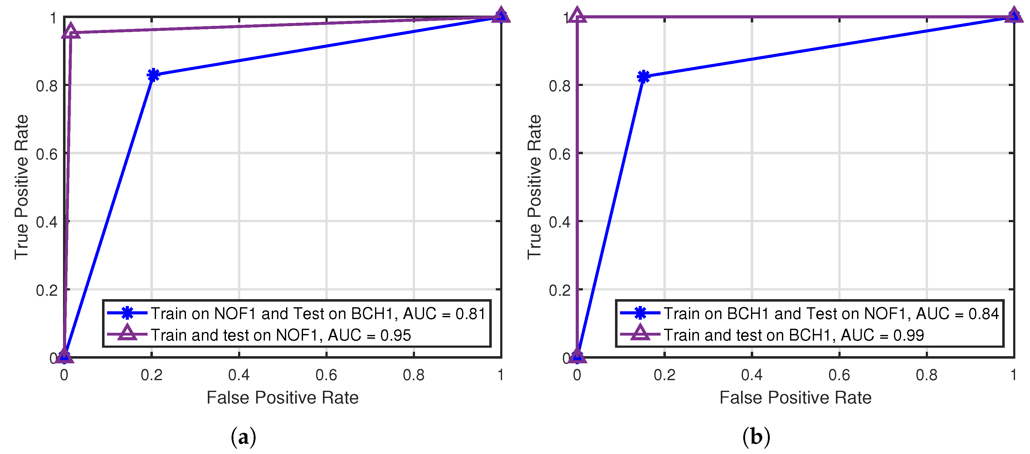
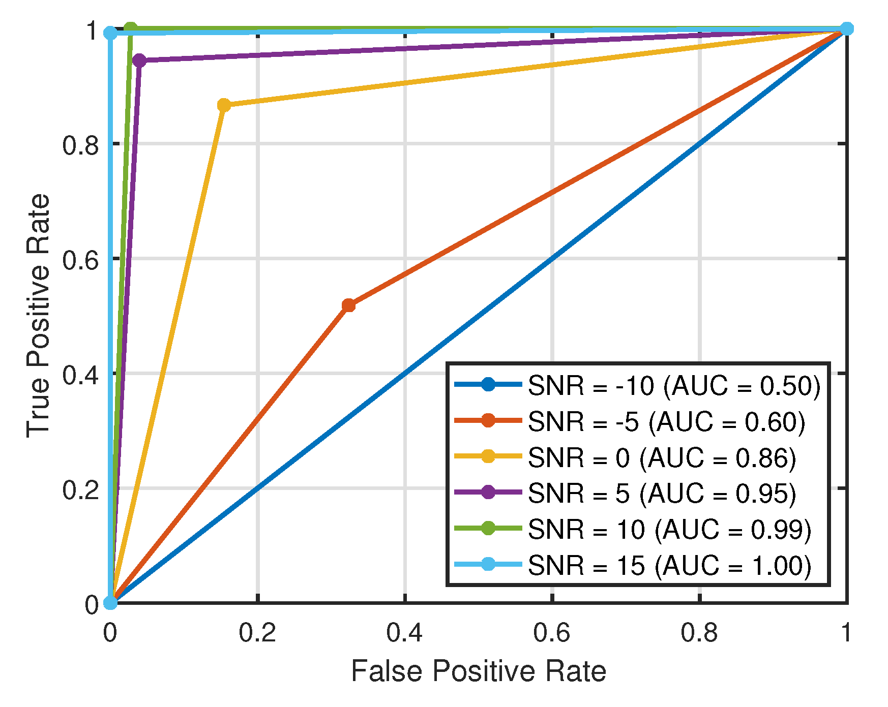
5.3. Robustness Analysis Under UWA Environment Mismatches

This subsection examines the performance of the proposed model under channel environment mismatches, a crucial factor in real-world UWA communication systems. In Figure 21a, training and testing on the same channel (NOF1) results in a substantial decrease in BER, reaching around ${10}^{-2}$ at $\mathrm{SNR}=10\mathrm{dB}$, showcasing the model’s optimal performance when channel conditions align. However, when trained on NOF1 and tested on BCH1, the BER remains much higher, with a clear performance drop as the SNR increases, reflecting the model’s struggle with mismatched environments.

Similarly, Figure 22 illustrates the drastic difference in performance between matching and mismatched environments. In Figure 22a (BCH1), the AUC drops from 0.95 (same channel) to 0.81 (mismatched), confirming that channel mismatch significantly impairs the model’s classification ability. A similar trend is seen in Figure 22b (BCH1), where the AUC falls from 0.99 to 0.83 under mismatched conditions, further emphasizing the challenge of generalizing across diverse channels. These results underline the importance of training on a variety of channels or adopting a transfer learning technique. With transfer learning, the model can leverage knowledge from one environment and adapt it to a new, unseen channel, significantly enhancing its robustness and real-world applicability.

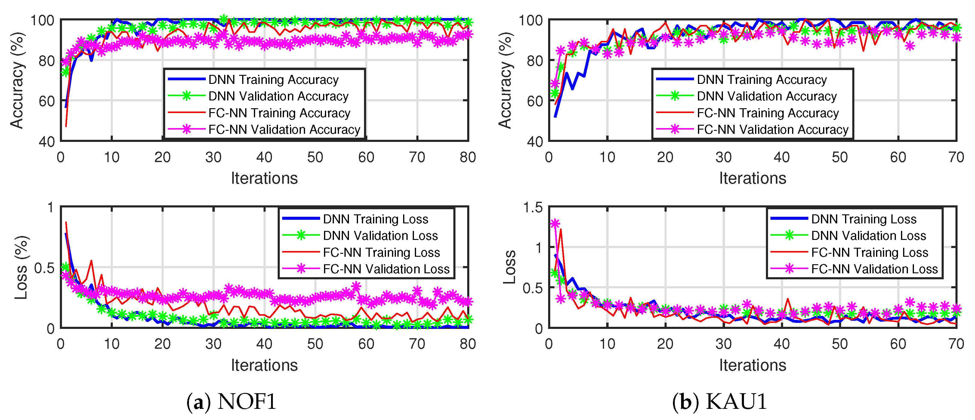
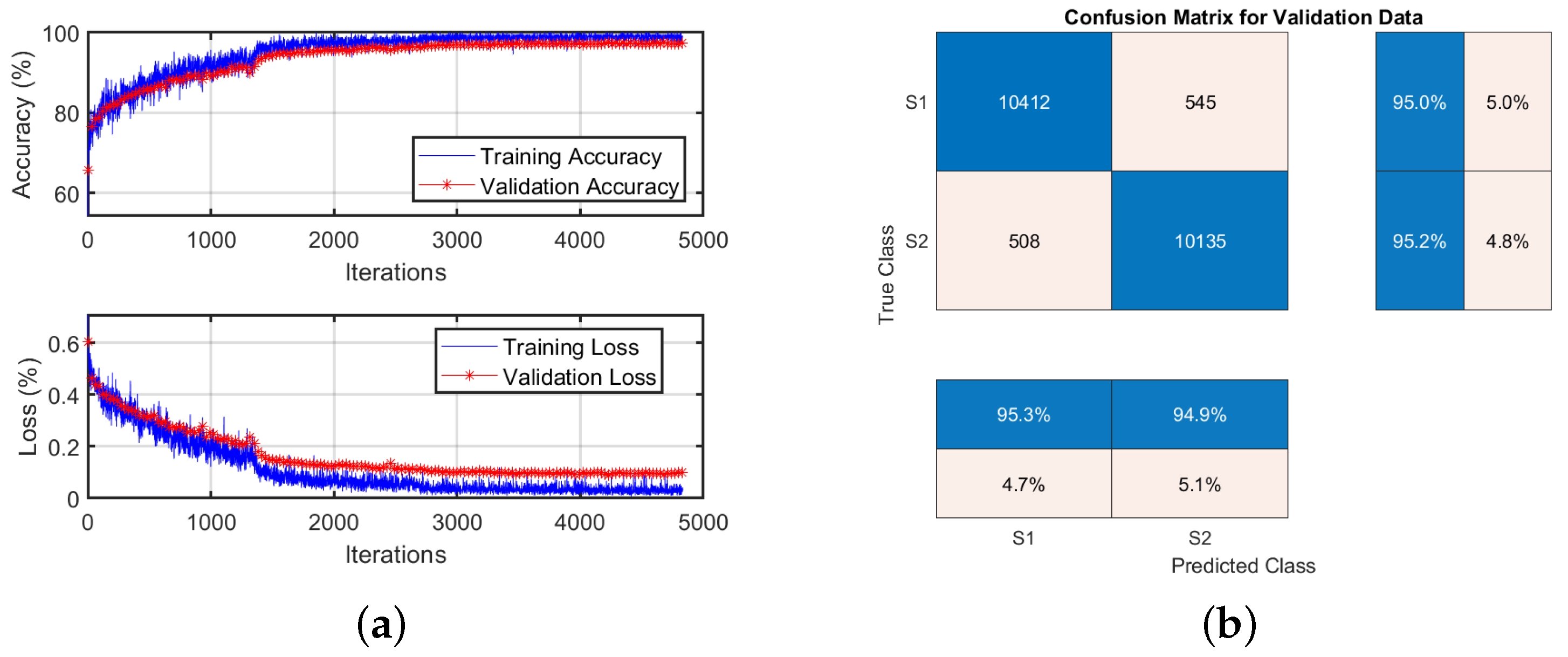
5.4. Pre-Trained Model Analysis

It is always important that a pre-trained model perform well on the training data before testing on new or target data. The key importance remains its generalization capability from the training data to unseen environments and tasks. If a model generalizes poorly to the training data, it would imply that the learning process failed to capture the underlying patterns in the data; hence, there might be a possibility of failure in performance when dealing with the target data. Good performance on training data, when combined with good results on the validation data, is a positive indication that general features have been learned by the model and may generalize well on new, unseen data, becoming suitable for real-world applications.

Figure 23a plots the training performance of the pre-trained model, in which the accuracy increases and the loss decreases in a systematic way during training. The model’s accuracy over the training set increases steadily and eventually well over 95%, indicating good learning. Much more importantly, the validation accuracy (plotted in red) is a measure of the model’s performance over unseen data. The comparable training and validation accuracy tells us that the model is not overfitted and has learned features that generalize sufficiently well. In Figure 23b, the confusion matrix of the pre-trained model shows its performance in predicting the channel conditions for validation data. Here, the model demonstrates high accuracy of 95% for S1 and 95.2% for S2, which is indicative of a robust model. The misclassification rates are also relatively low (5% for S1 and 4.8% for S2), suggesting that the model has learned to distinguish between the two conditions with reasonable accuracy. These results are important because they confirm the model’s ability to perform well, not only on the training data but also on new data (validation data). This means the model has successfully learned the critical features of the problem and can generalize to different conditions, which is vital for deployment in real-world scenarios, especially when using transfer learning for target data.

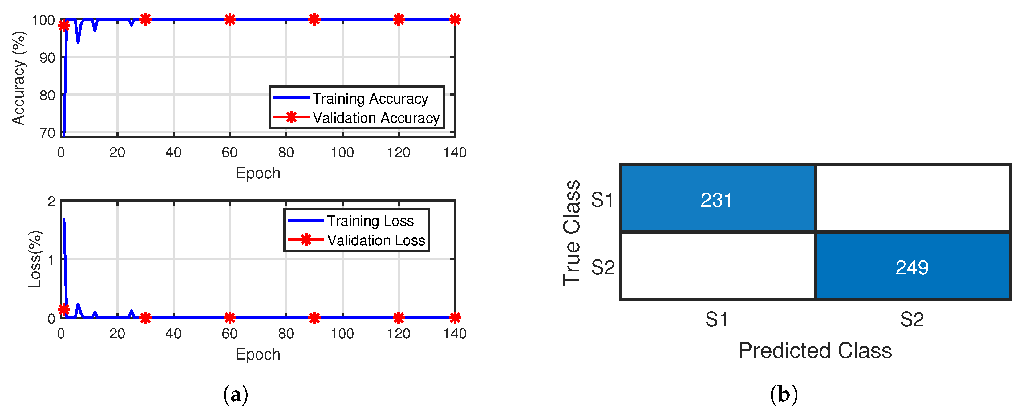
5.5. Transfer Learning Model Performance on Qingdao Lake Data

5.5.1. Comparative Study with and Without Transfer Learning

The results presented in Figure 24 and Figure 25 elucidate the striking differences in performance between the proposed TL approach and the scenario without transfer learning (no fine-tuning). In this context, “No TL” refers to applying the pre-trained model directly to the Qingdao Lake target data without fine-tuning, whereas “With TL” involves adapting the pre-trained model specifically for the target environment through fine-tuning. The Figure 24 and Figure 25 collectively demonstrate the efficacy of transfer learning in addressing the challenges posed by complex UWA environments. As depicted in Figure 24, the BER performance of the TL and without-TL models diverges significantly across varying SNR levels. For the without-TL model, the BER stagnates around 1 across all SNRs, including $\mathrm{SNR}=15\mathrm{dB}$, indicating an almost complete inability to generalize to the Qingdao Lake environment. The lack of fine-tuning means the pre-trained weights fail to adapt to the new channel characteristics, resulting in a model that is effectively non functional under these conditions. Conversely, the TL model demonstrates exceptional adaptability, achieving a BER of ${10}^{-2.0}$ (BER $\approx 0.001$) at $\mathrm{SNR}=10\mathrm{dB}$, and BER reaches $\approx 0$ at $\mathrm{SNR}=15\mathrm{dB}$, representing an improvement over the without-TL approach. Even at moderate SNR levels such as $SNR=0\mathrm{dB}$, the TL model achieves a BER of 0.08, while the without TL model remains at 0.9. This substantial reduction in BER underscores the TL model’s capacity to exploit the improved signal conditions effectively, while without TL, the performance stagnates due to its inability to adjust to the nonlinear and dynamic nature of the target environment. Figure 24b further illustrates the superiority of the TL model through a comparison of ROC curves and AUC values. The without-TL model achieves an AUC of only 0.45, which is barely above random guessing and reflects its poor discriminatory power. This is a direct consequence of the model’s inability to leverage the underlying structure of the target data due to the absence of fine-tuning. In stark contrast, the TL model achieves a perfect AUC of 1.00, indicating near optimal classification performance and a complete ability to separate the classes under all conditions. For reference, the FC-NN achieves a respectable AUC of 0.95, but it still falls short of the TL model. These results clearly highlight that fine-tuning the pre-trained model enables it to align its feature-extraction capabilities with the specific characteristics of the Qingdao Lake data, thereby achieving unparalleled performance.

The impact of transfer learning is further quantified in Figure 25. Key classification metrics include accuracy, precision, recall, F1 score, and MCC, all of which take values very close to 1.0, hence justifying the reliability of the TL model; specifically, the accuracy of the TL model approaches 1.0, while the without-TL model approaches 0.6, with evidence for frequent misclassifications. Precision and recall for the TL model are also close to perfection, showing that it can maximally increase the number of true positive predictions by allowing minimum false positives and false negatives. In contrast, the model without TL exhibited precision and recall values around 0.6, indicating a lack of confidence in its predictions. While the F1 score, representing a balanced measure of precision and recall, reaches 1.0 for the TL model but only 0.5 for the without-TL model, this underlines the notably inferior trade-offs the latter does between these metrics. Most importantly, the MCC of the TL model is 1.0, showing a perfect correlation between predicted and true classes, whereas for the without-TL model, the MCC is about 0.1, reflecting a random prediction behavior. These results highlight the fact that fine-tuning not only improves feature extraction but also ensures that the model learns class-specific discrimination important for robust classification.

5.5.2. Comparative Study of Transfer Learning on Target Data

The results presented in Figure 26, Figure 27 and Figure 28 demonstrate the effectiveness and robustness of the proposed TL model when applied to the Qingdao Lake target data. These figures showcase the model’s training progress, classification performance, and comparative evaluation against existing methods under varying SNR conditions. Figure 26a illustrates the training and validation accuracy and loss trends of the transfer learning model over 140 epochs. The training accuracy quickly approaches 100%, stabilizing within a few epochs, while the validation accuracy also converges to 100% with negligible divergence. This rapid convergence highlights the benefits of leveraging pre-trained weights, which provide a strong initialization and allow the model to adapt efficiently to the target data.

Such robustness is further reinforced in the trend of training and validation loss. Both show sharp decreases within the initial epochs and stabilize close to 0%, with minor fluctuations in the validation loss. This correspondence between training and validation metrics is indicative of good generalization. These results confirm that transfer learning allows for the extraction of meaningful features in UWA communication environments. The confusion matrix shown in Figure 26b depicts the performance evaluation of the model using the validation dataset. Indeed, the model predicted almost perfectly, with 231 correct samples in S1 and 249 samples correctly classified in S2 with few misclassifications. This translates into 98.3% class classification accuracy for S1 and 98.0% for S2, meaning performance was balanced between both classes and unbiased. The high accuracy of classification with low misclassification rates underlines the adaptability of the model to the Qingdao Lake environment. It tends to fine-tune the pre-trained weights and captures the distinctive characteristics of each class while canceling channel distortions. This performance underlines the adequacy of the transfer learning approach for robust underwater communication. The ROC curves of the transfer learning model on different SNRs are shown in Figure 27. At $SNR=-10\mathrm{dB}$, the AUC is equal to 0.50 since noise dominates the performance and tends toward random guessing. As SNR increases, AUC increases significantly, reaching 0.86 at $SNR=0\mathrm{dB}$, which is indicative of effective pattern recognition under a moderate quality of signal. For higher SNRs, the performance of the model is close to optimal: AUC = 0.95 at $SNR=5\mathrm{dB}$, AUC = 0.99 at $SNR=10\mathrm{dB}$, and AUC = 1.00 at $SNR=15\mathrm{dB}$. These results underline how the transfer learning model could exploit an increase in signal quality and improve classification accuracy. Achieving complete discrimination for high SNRs upper bounds the performance and shows the robustness and suitability of the model for real-world UWA systems.

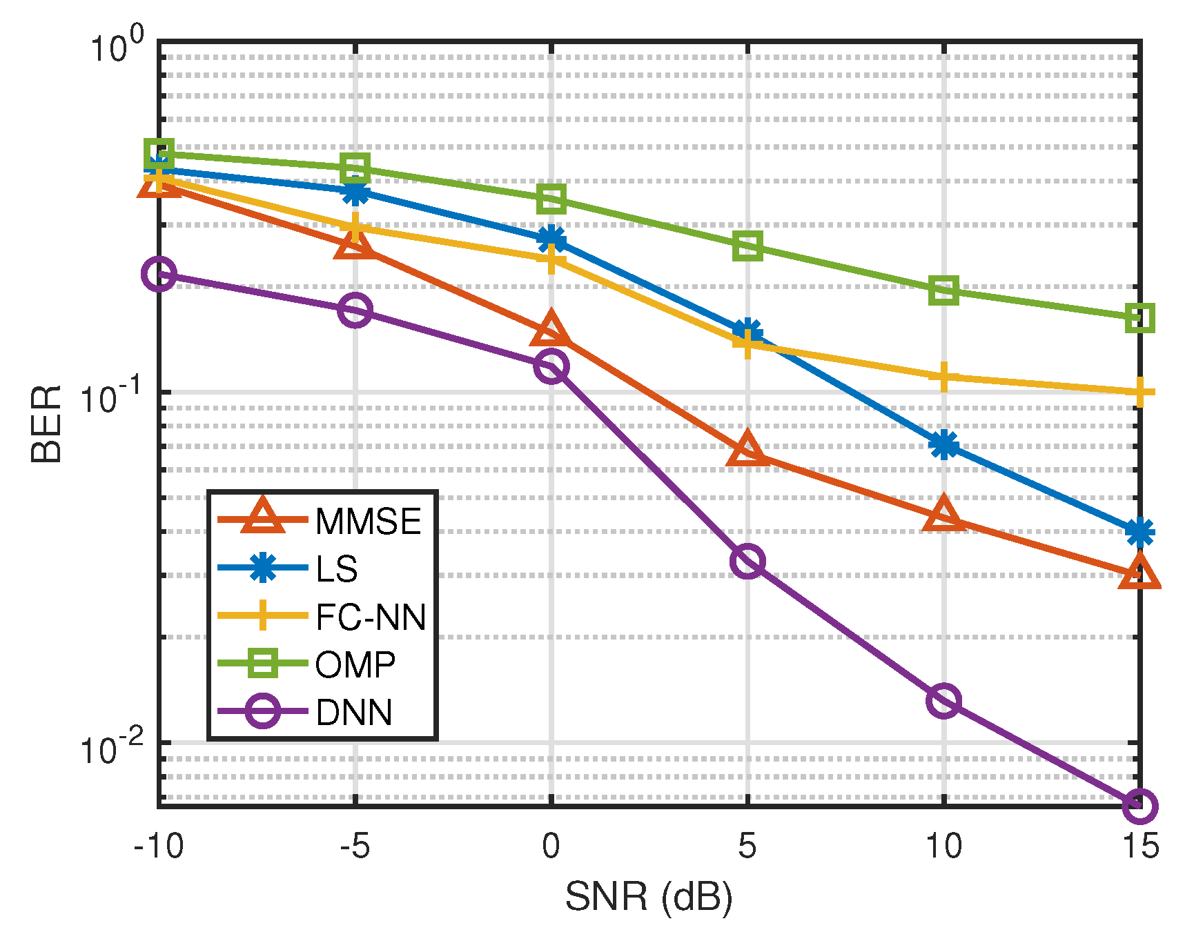
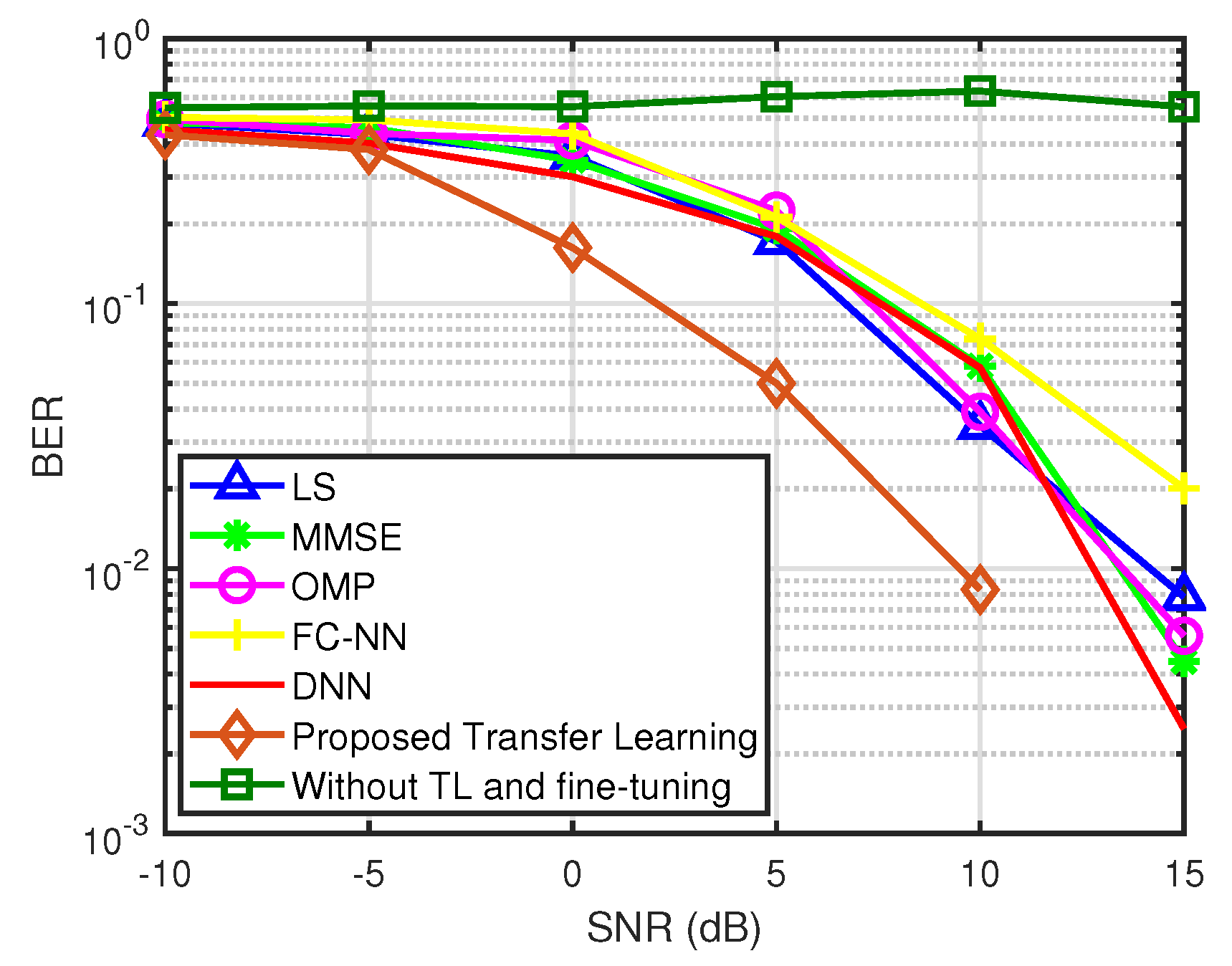
5.5.3. Evaluation of the Proposed Transfer Learning Model with BER Performance in an Extended Range of SNR

Figure 28 presents a comprehensive comparison of the BER performance of the proposed TL model against conventional and deep learning-based channel-estimation techniques. At $SNR=-10\mathrm{dB}$, the transfer learning model achieves a BER of $0.25$, outperforming the DNN (BER = $0.3$) and FC-NN (BER = $0.4$). In stark contrast, traditional methods such as OMP, LS, and MMSE estimators exhibit poor performance, with BER values approaching $0.7$, indicating their inability to effectively handle the highly nonlinear and time-varying nature of UWA channels. As the SNR increases, the transfer learning model maintains a significant performance advantage. At $SNR=0\mathrm{dB}$, it achieves a BER of $0.12$, surpassing the DNN (BER = $0.25$) and FC-NN (BER = $0.3$). At higher SNRs, the superiority of transfer learning becomes even more evident. At $SNR=10\mathrm{dB}$, the proposed model attains a BER of $0.009$, compared to $0.05$ for DNN and $0.06$ for FC-NN, while LS and MMSE remain above $0.07$ even in high SNR scenarios. At $SNR=15\mathrm{dB}$, the transfer learning model reaches an impressive BER of 0, further underscoring its robustness and adaptability to varying environmental conditions. The LS estimator, despite its simplicity, is highly sensitive to noise and fails to capture the inherent nonlinearities of the UWA channel. MMSE, while more robust, requires prior knowledge of the channel’s autocorrelation function and noise variance, making it computationally prohibitive and impractical for real-time applications. Similarly, OMP, a sparsity-based method, struggles in dynamic underwater environments due to its reliance on an accurate sparsity assumption, which is often violated in real-world UWA scenarios. While deep learning based models such as FC-NN and DNN demonstrate improved performance by learning complex channel representations, they are inherently limited by their dependence on large, representative training datasets. A key drawback of these models is their performance degradation when applied to environments different from those seen during training, a challenge commonly referred to as model mismatch. This limitation severely restricts their adaptability in diverse and evolving underwater conditions. The proposed TL approach addresses these challenges by leveraging a pre-trained model, initially trained on a source dataset, and fine-tuning it with minimal new data from the target environment (e.g., Qingdao Lake). This enables the model to retain essential learned features while adapting to the unique characteristics of a new underwater communication channel, thereby reducing the need for extensive retraining. Unlike traditional deep learning models that require large-scale labeled data, TL significantly enhances generalization, ensuring robust performance across varying conditions while maintaining computational efficiency. In summary, the results highlight the transformative impact of transfer learning in UWA channel estimation. By overcoming the limitations of conventional methods and mitigating the data dependency of standard deep learning approaches, transfer learning emerges as a state-of-the-art solution, ensuring high reliability and accuracy in practical underwater communication systems.

5.6. Computational Complexity Analysis

The computational complexity of different benchmark methods, including LS, MMSE, FC-NN, and DNN, is compared against the proposed transfer learning model. The complexity of each method is analyzed based on the number of sub-carriers $K_c$, number of data indices $K_{data}$, and the architectural parameters of deep learning-based models. The LS algorithm remains one of the most computationally efficient methods with a complexity of:

$$O(K_c^2+K_c+K_{data}),$$

where $K_c$ is number of sub-carriers, making it feasible for moderate-scale systems, its reliance on traditional channel-estimation techniques limits its accuracy, particularly in dynamic and nonlinear communication environments. The additional $O\left(K_c\right)$ and $O\left(K_{data}\right)$ terms account for the equalization and demodulation steps, making LS an efficient but relatively less accurate approach. The MMSE algorithm, known for its superior performance by minimizing the mean square error, incurs a significantly higher computational cost:

$$O(K_c^3+K_c+K_{data}).$$

The cubic dependence on $K_c$ arises due to matrix inversion operations, making MMSE computationally expensive. Despite its improved accuracy over LS, the practical implementation of MMSE in real-time systems is often constrained by its high computational demand. The introduction of neural networks for channel estimation, such as FC-NN, shifts the computational paradigm towards learning-based approaches. The complexity of the FC-NN model is given by:

$$O(L_f\times K_c^2).$$

Here, $L_f$ represents the number of fully connected layers. Unlike LS and MMSE, which rely on explicit mathematical formulations, FC-NN learns an implicit mapping of channel conditions, reducing the dependency on traditional equalization methods. However, the fully connected nature of this architecture results in a quadratic complexity with respect to $K_c$, making it computationally demanding as the number of sub-carriers increases. The DNN model improves upon FC-NN by introducing hierarchical feature extraction, with its complexity formulated as:

$$O(L_f\times K_c^2)+O(L_d\times K_c),$$

where $L_d$ represents the number of dense layers in addition to the fully connected layers. The additional term $O(L_d\times K_c)$ allows DNN to capture more abstract representations, improving performance in complex environments. However, the dependency on deep fully connected layers leads to high parameterization, increasing training and inference time. The proposed transfer learning model significantly optimizes computational efficiency by leveraging pre-trained feature representations, thereby reducing the number of trainable parameters. The complexity is formulated as:

$$O(L_c\times K_c)+O(L_f\times K_c^2),$$

where $L_c$ represents the number of convolutional layers. The presence of convolutional layers enables hierarchical feature extraction, drastically reducing computational overhead compared to fully connected networks. Furthermore, by freezing convolutional layers during fine-tuning, the complexity is effectively reduced to:

$$O(L_f\times K_c^2),$$

as only the fully connected layers are updated during transfer learning. This approach allows the model to generalize efficiently to new environments while significantly reducing computational demand. The use of pre-trained weights mitigates the need for learning low-level features from scratch, making transfer learning an optimal trade-off between complexity and performance. A comparative summary of the computational complexity of each method is provided in

Table 10. Computational complexity comparison.

Algorithm	Complexity
LS	$O(K_c^2+K_c+K_{data})$
MMSE	$O(K_c^3+K_c+K_{data})$
FC-NN	$O(L_f\times K_c^2)$
DNN	$O(L_f\times K_c^2)+O(L_d\times K_c)$
Proposed Transfer Learning	$O(L_c\times K_c)+O(L_f\times K_c^2)$
Fine-Tuned Transfer Learning	$O(L_f\times K_c^2)$ (Frozen Conv. Layers)

.

The analysis in Table 10 highlights the scalability advantages of transfer learning over conventional methods. Although LS remains computationally efficient, its limited accuracy makes it unsuitable for complex scenarios. MMSE offers improved accuracy at a significant computational cost, making it impractical for real-time applications with large subcarrier counts. FC-NN and DNN mitigate some of these issues, but introduce high parameterization costs due to the reliance on fully connected layers. The proposed transfer learning model, particularly in its fine-tuned configuration, provides an optimal balance, leveraging pre-trained features to reduce computational overhead while maintaining high accuracy. By freezing convolutional layers during fine-tuning, the computational burden is significantly reduced, making the approach suitable for real-time UWA communication systems.

6. Conclusions

In this work, we proposed a novel TL-based pre-trained model for OFDM-based UWA communication systems. Our approach addresses the major issue of performance degradation caused by model mismatch in unseen environments, which is common in traditional DNN models, by successful adaptation with minimal retraining. By training over diverse realistic channel conditions of real-world channels in the watermark channels and considering SNR variations, the proposed model exhibits superior robustness and generalization. In addition, our real-world experiments carried out in Qingdao Lake, Hangzhou, China, validate the proposed model. It demonstrates the capabilities of the TL-based OFDM receiver in dealing with severe UWA conditions, outperforming traditional methods like LS, MMSE, OMP, and DNN with respect to BER and adaptability for different channel conditions. The proposed TL approach stands out as an effective solution to model mismatch, thus ensuring real-world practical deployment for any UWA communication system. Future work can be directed toward incorporating a wider range of environmental datasets and further fine-tuning the model to improve performance in even more dynamic and unpredictable underwater scenarios.

References

1. Li, Z.; Chitre, M.; Stojanovic, M. Underwater acoustic communications. Nat. Rev. Electr. Eng. 2024, 2, 83–95. [Google Scholar] [CrossRef]
2. Men, W.; Wang, J.; Dong, B.; Hou, X.; Jiang, C.; Ren, Y. OFDM-Based Underwater Integrated Sensing and Communication: Receiver Design for Doubly Spread Acoustic Channels. IEEE Trans. Commun. 2025. [Google Scholar] [CrossRef]
3. Wan, L.; Deng, S.; Chen, Y.; Cheng, E. Sparse channel estimation for underwater acoustic OFDM systems with super-nested pilot design. Signal Process. 2025, 227, 109709. [Google Scholar] [CrossRef]
4. Zhou, M.; Sun, H.; Wang, J.; Xie, Z.; Feng, X. Channel Estimation for Underwater Acoustic OFDM Communications: Recent Advances. Recent Patents Eng. 2025, 19, E050723218434. [Google Scholar] [CrossRef]
5. Feng, X.; Wang, J.; Sun, H.; Qi, J.; Qasem, Z.A.H.; Cui, Y. Channel estimation for underwater acoustic OFDM communications via temporal sparse Bayesian learning. Signal Process. 2023, 207, 108951. [Google Scholar] [CrossRef]
6. Tian, T.; Yang, K.; Wu, F.-Y.; Zhang, Y. Channel estimation for underwater acoustic communications in impulsive noise environments: A sparse, robust, and efficient alternating direction method of multipliers-based approach. Remote Sens. 2024, 16, 1380. [Google Scholar] [CrossRef]
7. Manasa, B.M.R.; Venugopal, P. A systematic literature review on channel estimation in MIMO-OFDM system: Performance analysis and future direction. J. Opt. Commun. 2024, 45, 589–614. [Google Scholar] [CrossRef]
8. Junejo, N.U.R.; Sattar, M.; Adnan, S.; Sun, H.; Adam, A.B.M.; Hassan, A.; Esmaiel, H. A survey on physical layer techniques and challenges in underwater communication systems. J. Mar. Sci. Eng. 2023, 11, 885. [Google Scholar] [CrossRef]
9. Farzamnia, A.; Hlaing, N.W.; Haldar, M.K.; Rahebi, J. Channel estimation for sparse channel OFDM systems using least square and minimum mean square error techniques. In Proceedings of the International Conference on Engineering and Technology (ICET), Antalya, Turkey, 21–23 August 2017; pp. 1–5. [Google Scholar] [CrossRef]
10. Kumar, A. A new optimized least-square sparse channel estimation scheme for underwater acoustic communication. Int. J. Commun. Syst. 2023, 36, e5436. [Google Scholar] [CrossRef]
11. Kumar, A.; Kumar, P. An improved sparsity-aware normalized least-mean-square scheme for underwater communication. Etri J. 2023, 45, 379–393. [Google Scholar] [CrossRef]
12. Alraie, H.; Ishii, K. Channel estimation using pilot-assisted OFDM for underwater acoustic communication. J. Robot. Netw. Artif. Life 2023, 10, 160–165. [Google Scholar] [CrossRef]
13. Chen, P.; Rong, Y.; Nordholm, S.; He, Z. Joint channel and impulsive noise estimation in underwater acoustic OFDM systems. IEEE Trans. Veh. Technol. 2017, 66, 10567–10571. [Google Scholar] [CrossRef]
14. Liu, D.N.; Yerramalli, S.; Mitra, U. On efficient channel estimation for underwater acoustic OFDM systems. In Proceedings of the 4th International Workshop Underwater Acoustic Digital Signal Processing, Berkeley, CA, USA, 3 November 2009; Volume 16, no. 1, pp. 4–10. [Google Scholar] [CrossRef]
15. Jiang, W.; Diamant, R. Long-range underwater acoustic channel estimation. IEEE Trans. Wirel. Commun. 2023, 22, 6267–6282. [Google Scholar] [CrossRef]
16. Murad, M.; Tasadduq, I.A.; Otero, P. Pilots based LSE channel estimation for underwater acoustic OFDM communication. In Proceedings of the 2020 Global Conference on Wireless and Optical Technologies (GCWOT), Malaga, Spain, 6–8 October 2020; pp. 1–6. [Google Scholar] [CrossRef]
17. Tian, T.; Wu, F.-Y.; Yang, K. Estimation of underwater acoustic channel via block-sparse recursive least-squares algorithm. In Proceedings of the 2019 IEEE International Conference on Signal Processing, Communications and Computing (ICSPCC), Dalian, China, 20–22 September 2019; pp. 1–6. [Google Scholar] [CrossRef]
18. Junejo, N.U.R.; Esmaiel, H.; Sun, H.; Qasem, Z.A.H.; Wang, J. Pilot-based adaptive channel estimation for underwater spatial modulation technologies. Symmetry 2019, 11, 711. [Google Scholar] [CrossRef]
19. Song, S.; Lim, J.-S.; Baek, S.J.; Sung, K.M. Variable forgetting factor linear least squares algorithm for frequency selective fading channel estimation. IEEE Trans. Veh. Technol. 2002, 51, 613–616. [Google Scholar] [CrossRef]
20. Qiao, G.; Babar, Z.; Ma, L.; Liu, S.; Wu, J. MIMO-OFDM underwater acoustic communication systems—A review. Phys. Commun. 2017, 23, 56–64. [Google Scholar] [CrossRef]
21. Ma, X.-F.; Zhao, C.-H.; Qiao, G. The underwater acoustic OFDM channel estimation based on wavelet and MMSE. In Proceedings of the 2009 WRI International Conference on Communications and Mobile Computing, Kunming, China, 6–8 January 2009; IEEE: Piscataway, NJ, USA, 2009; Volume 2, pp. 573–577. [Google Scholar] [CrossRef]
22. Zhang, Y.; Li, J.; Zakharov, Y.; Li, X.; Li, J. Deep learning-based underwater acoustic OFDM communications. Appl. Acoust. 2019, 154, 53–58. [Google Scholar] [CrossRef]
23. Jiang, R.; Wang, X.; Cao, S.; Zhao, J.; Li, X. Deep neural networks for channel estimation in underwater acoustic OFDM systems. IEEE Access 2019, 7, 23579–23594. [Google Scholar] [CrossRef]
24. Liu, S.; Adil, M.; Ma, L.; Mazhar, S.; Qiao, G. DenseNet-Based Robust Channel Estimation in OFDM for Improving Underwater Acoustic Communication. IEEE J. Ocean. Eng. 2025, 50, 1518–1537. [Google Scholar] [CrossRef]
25. Xu, W.; Zhong, Z.; Be’ery, Y.; You, X.; Zhang, C. Joint neural network equalizer and decoder. In Proceedings of the 2018 15th International Symposium on Wireless Communication Systems (ISWCS), Lisbon, Portugal, 28–31 August 2018; IEEE: Piscataway, NJ, USA, 2018; pp. 1–5. [Google Scholar]
26. Zhang, Y.; Li, C.; Wang, H.; Wang, J.; Yang, F.; Meriaudeau, F. Deep learning aided OFDM receiver for underwater acoustic communications. Appl. Acoust. 2022, 187, 108515. [Google Scholar] [CrossRef]
27. Liu, S.; Yan, H.; Ma, L.; Liu, Y.; Han, X. UACC-GAN: A Stochastic Channel Simulator for Underwater Acoustic Communication. IEEE J. Ocean. Eng. 2024, 49, 1605–1621. [Google Scholar] [CrossRef]
28. Zhang, Y.; Chang, J.; Liu, Y.; Xing, L.; Shen, X. Deep learning and expert knowledge-based underwater acoustic OFDM receiver. Phys. Commun. 2023, 58, 102041. [Google Scholar] [CrossRef]
29. Zhang, J.; Cao, Y.; Han, G.; Fu, X. Deep neural network-based underwater OFDM receiver. IET Commun. 2019, 13, 1998–2002. [Google Scholar] [CrossRef]
30. Hassan, S.; Chen, P.; Rong, Y.; Chan, K.Y. Underwater acoustic OFDM receiver using a regression-based deep neural network. In Proceedings of the OCEANS 2022, Hampton Roads, VA, USA, 17–20 October 2022; IEEE: Piscataway, NJ, USA, 2022; pp. 1–6. [Google Scholar]
31. Wang, Z.; Liu, L.; Cheng, Z.; Wang, J. Intelligent Receiver Design for Underwater Acoustic OFDM Communication Based on LSTM Networks. In Proceedings of the 2023 IEEE International Conference on Signal Processing, Communications and Computing (ICSPCC), Zhengzhou, China, 14–17 November 2023; IEEE: Piscataway, NJ, USA, 2023; pp. 1–6. [Google Scholar]
32. Guo, J.; Guo, T.; Li, M.; Wu, T.; Lin, H. Underwater-Acoustic-OFDM Channel Estimation Based on Deep Learning and Data Augmentation. Electronics 2024, 13, 689. [Google Scholar] [CrossRef]
33. Jiang, P.; Wang, T.; Han, B.; Gao, X.; Zhang, J.; Wen, C.-K.; Jin, S.; Li, G.Y. AI-aided online adaptive OFDM receiver: Design and experimental results. IEEE Trans. Wirel. Commun. 2021, 20, 7655–7668. [Google Scholar] [CrossRef]
34. Zhang, Y.; Li, J.; Zakharov, Y.; Sun, D.; Li, J. Underwater Acoustic OFDM Communications Using Deep Learning. 2018. Available online: https://eprints.soton.ac.uk/426097/1/FCAC_Deeplearning_OFDM_finally.pdf (accessed on 20 May 2025).
35. Alves, W.; Correa, I.; González-Prelcic, N.; Klautau, A. Deep transfer learning for site-specific channel estimation in low-resolution mmWave MIMO. IEEE Wirel. Commun. Lett. 2021, 10, 1424–1428. [Google Scholar] [CrossRef]
36. Hong, J.; Cheng, H.; Zhang, Y.D.; Liu, J. Detecting cerebral microbleeds with transfer learning. Mach. Vis. Appl. 2019, 30, 1123–1133. [Google Scholar] [CrossRef]
37. Das, A.K.; Pramanik, A. A Survey Report on Underwater Acoustic Channel Estimation of MIMO-OFDM System. In Proceedings of the International Conference on Frontiers in Computing and Systems: COMSYS 2020, Jalpaiguri, India, 13–15 January 2020; Springer: Singapore, 2021; pp. 745–753. [Google Scholar] [CrossRef]
38. Liu, L.; Zhang, Y.; Zhang, P.; Zhou, L.; Li, J.; Jin, J.; Zhang, J.; Lv, Z. PN sequence based doppler and channel estimation for underwater acoustic OFDM communication. In Proceedings of the 2016 IEEE International Conference on Signal Processing, Communications and Computing (ICSPCC), Hong Kong, China, 5–8 August 2016; pp. 1–6. [Google Scholar] [CrossRef]
39. Jan, M.; Mazhar, S.; Adil, M.; Muhammad, A.; Gang, Q. Integration of Deep Neural Networks and Local mean decomposition for accurate underwater acoustic channel estimation. In Proceedings of the 2023 20th International Bhurban Conference on Applied Sciences and Technology (IBCAST), Bhurban, Murree, Pakistan, 22–25 August 2023; IEEE: Piscataway, NJ, USA, 2023; pp. 866–871. [Google Scholar]
40. Liu, H.; Ma, L.; Wang, Z.; Qiao, G. Channel prediction for underwater acoustic communication: A review and performance evaluation of algorithms. Remote Sens. 2024, 16, 1546. [Google Scholar] [CrossRef]
41. Adil, M.; Liu, S.; Mazhar, S.; Jan, M.; Khan, A.Y.; Bilal, M. A Fully Connected Neural Network Driven UWA Channel Estimation for Reliable Communication. In Proceedings of the 2023 International Conference on Frontiers of Information Technology (FIT), Islamabad, Pakistan, 11–12 December 2023; IEEE: Piscataway, NJ, USA, 2023; pp. 310–315. [Google Scholar]
42. van Walree, P.A.; Socheleau, F.-X.; Otnes, R.; Jenserud, T. The watermark benchmark for underwater acoustic modulation schemes. IEEE J. Ocean. Eng. 2017, 42, 1007–1018. [Google Scholar] [CrossRef]
43. Cho, Y.S.; Kim, J.; Yang, W.Y.; Kang, C.G. MIMO-OFDM Wireless Communications with MATLAB; John Wiley and Sons: Hoboken, NJ, USA, 2010. [Google Scholar]
44. Zhang, Y.; Wang, H.; Li, C.; Meriaudeau, F. Data augmentation aided complex-valued network for channel estimation in underwater acoustic orthogonal frequency division multiplexing system. J. Acoust. Soc. Am. 2022, 151, 4150–4164. [Google Scholar] [CrossRef]
45. Hossin, M.; Sulaiman, M.N. A review on evaluation metrics for data classification evaluations. Data Min. Knowl. Manag. Process 2015, 5, 1–13. [Google Scholar] [CrossRef]
46. Miao, J.; Zhu, W. Precision–recall curve (PRC) classification trees. Evol. Intell. 2022, 15, 1545–1569. [Google Scholar] [CrossRef]
47. Yacouby, R.; Axman, D. Probabilistic extension of precision, recall, and F1 score for more thorough evaluation of classification models. In Proceedings of the First Workshop on Evaluation and Comparison of NLP Systems, Online, 20 November 2020; pp. 79–91. [Google Scholar] [CrossRef]
48. Powers, D.M. Evaluation: From precision, recall and F-measure to ROC, informedness, markedness and correlation. arXiv 2020, arXiv:2010.16061. [Google Scholar] [CrossRef]
49. Chicco, D.; Jurman, G. The Matthews correlation coefficient (MCC) should replace the ROC AUC as the standard metric for assessing binary classification. BioData Min. 2023, 16, 4–10. [Google Scholar] [CrossRef] [PubMed]
50. Cao, C.; Chicco, D.; Hoffman, M.M. The MCC-F1 curve: A performance evaluation technique for binary classification. arXiv 2020, arXiv:2006.11278. [Google Scholar] [CrossRef]
51. Zhang, Y.; Wang, H.; Li, C.; Chen, X.; Meriaudeau, F. On the performance of deep neural network aided channel estimation for underwater acoustic OFDM communications. Ocean Eng. 2022, 259, 111518. [Google Scholar] [CrossRef]
Figure 2. Traditional deep learning-based UWA OFDM communication system, reproduced from [22], Applied Acoustics, 2019.
Jmse 13 01284 g002
Figure 3. Comparison of individual data training in DL vs. knowledge reuse in TL.
Jmse 13 01284 g003
Figure 4. The process of data collection.
Jmse 13 01284 g004
Figure 5. The process of data concatenation.
Jmse 13 01284 g005
Figure 6. The proposed TL approach.
Jmse 13 01284 g006
Figure 7. The configuration of different watermark channels.
Jmse 13 01284 g007
Figure 8. Configuration of Qingdao Lake channel.
Jmse 13 01284 g008
Figure 9. The CIR of different channels.
Jmse 13 01284 g009
Figure 10. The TVIR of different channels.
Jmse 13 01284 g010
Figure 11. The The characteristics of the Qingdao Lake channel. Each subfigure (af) shows the time evolution of the channel impulse response, the delay-Doppler spread, and the power delay profile, highlighting the channel’s temporal and multipath variability.
Jmse 13 01284 g011
Figure 12. Hardware connection block diagram of proposed system.
Jmse 13 01284 g012
Figure 13. Training and validation accuracy and loss analysis, when trained and tested on the same channel (where each of NOF1 and KAU1 channels are split into training and testing sets).
Jmse 13 01284 g013
Figure 14. Confusion metrics of FCNN at SNR 15 (dB), when trained and tested on a same channel.
Jmse 13 01284 g014
Figure 15. Confusion metrics of DNN at SNR 15 (dB), when trained and tested on a same channel across different channels.
Jmse 13 01284 g015
Figure 16. ROC curve of DNN for different SNR, for the channel NOF1.
Jmse 13 01284 g016
Figure 17. ROC curve of DNN for different SNR, for the channel BCH1.
Jmse 13 01284 g017
Figure 18. Performance metrics of FCNN and DNN at 15 SNR, when trained and tested on the same channel across different channels.
Jmse 13 01284 g018
Figure 19. BER vs. SNR for an OFDM receiver with single-channel training and testing on the BCH1 channel.
Jmse 13 01284 g019
Figure 20. BER vs. SNR for an OFDM receiver with single-channel training and testing on the NOF1 channel.
Jmse 13 01284 g020
Figure 21. BER vs. SNR under channel environment mismatches. (a,b) compare training and testing on same vs. different channel scenarios between NOF1 and BCH1.
Jmse 13 01284 g021
Figure 22. ROC under channel environment mismatches, SNR is 15 dB. (a,b) compare training and testing on same vs. different channel scenarios between NOF1 and BCH1.
Jmse 13 01284 g022
Figure 23. Training progress and confusion matrix of pre-trained model. (a) Training progress of pre-trained model; (b) Confusion Matrix of pre-trained model for Validation Data.
Jmse 13 01284 g023
Figure 24. Comparison between BER vs. SNR and ROC curve for pre-trained and transfer learning models. (a) BER vs. SNR comparison of pre-trained vs. transfer learning with target data. (b) ROC curve comparison between a pre-trained model without fine-tuning on target data and a transfer learning approach with target data adaptation.
Jmse 13 01284 g024
Figure 25. Performance matrix comparison between a pre-trained model without fine-tuning on target data and a transfer learning approach with target data adaptation.
Jmse 13 01284 g025
Figure 26. Training progress and confusion matrix of the transfer learning model on Qingdao lake/target data. (a) Training and validation accuracy and loss of TL model on Qingdao lake/target data. (b) Confusion Matrix of TL model on Qingdao lake/target data.
Jmse 13 01284 g026
Figure 27. ROC curve of TL model on Qingdao lake/target data.
Jmse 13 01284 g027
Figure 28. BER vs. SNR of TL model on Qingdao lake/target data.
Jmse 13 01284 g028