Predefined-Performance Sliding-Mode Tracking Control of Uncertain AUVs via Adaptive Disturbance Observer

Abstract

In this paper, a sliding-mode control strategy incorporating prescribed features was systematically designed, resolving the dual challenges of trajectory tracking precision maintenance and disturbance attenuation for an AUV subjected to dynamic model inaccuracies and disturbances. To neutralize the impact of parametric uncertainties and environmental disturbances on the controlled plant, an adaptive finite-time sliding-mode disturbance observer (AFTSMDO), the upper bound of perturbations was not required for the proposed observer. Subsequently, by embedding error transformations and prescribed performance functions, we designed a novel sliding-mode surface. This surface ensured that tracking errors and their derivatives converge to specified regions within predefined temporal bounds, irrespective of initial configurations. This overcomes the longstanding limitations of traditional prescribed performance control methods and contributes to enhancing system performance. Finally, we conducted comparative simulation experiments with existing sliding-mode control methods to prove the practical viability and comparative advantage of the synthesized control methodology.

1. Introduction

With continuous advancements in ocean engineering [1,2], autonomous underwater vehicles (AUVs) are assuming an increasingly pivotal role in diverse domains, including marine scientific research, resource exploration, and environmental monitoring [3,4]. Within the realm of AUV applications, the capability to swiftly and accurately track trajectories emerges as a paramount concern [5]. Nevertheless, the dynamic modeling of AUVs exhibits pronounced nonlinearity and substantial interdependence with the unpredictable marine environment, encompassing factors such as currents, waves, and buoyancy [6]. Consequently, achieving trajectory tracking control for AUVs is far from straightforward and remains a central challenge within this field.

Known for its robustness, the SMC method is widely regarded as a viable means for addressing systems with parametric uncertainties and energy-bound external perturbations. Sliding-mode control achieves robust performance in uncertain systems through a discontinuous control law. This law forces the system state onto a designated sliding surface and subsequently constrains the state trajectory to evolve on this manifold. The system’s dynamics, while constrained to the sliding manifold, become invariant to a specific class of disturbances and uncertainties, known as “matched uncertainties”. During sliding motion, the controller inherently compensates for these matched perturbations without requiring their explicit measurement or knowledge, achieving inherent robustness [7]. Due to this advantage, several SMC strategies for AUVs have been proposed to ensure that the system’s output effectively tracks target trajectories [8,9,10]. However, the practical implementation of these approaches often relies on having the upper-bound information about uncertainty terms or applying large gains to suppress disturbances. By incorporating adaptive techniques into sliding mode control, it becomes possible to achieve online estimation of the upper bound of disturbances through adaptive update laws [11,12,13]. Nevertheless, the adaptive gains remain relatively conservative, inevitably resulting in energy wastage. In this study, we established a comprehensive disturbance observer that operates independently of information concerning disturbances and their derivative upper bounds. This observer provides the real-time estimation of integrated disturbances, effectively alleviating conservatism issues within the controller. Furthermore, it is worth noting that controllers designed based on a linear SM surface can only ensure the asymptotic error convergence to zero over infinite time, which cannot satisfy the urgent demand for rapid response in AUV trajectory tracking tasks [14].

Consisting of the nonlinear mapping of trajectory tracking errors and their temporal derivatives, terminal sliding-mode (TSM) methods can ensure that the trajectory regulation discrepancy of a feedback-controlled system converges in specified temporal bound [15,16,17]. However, the traditional TSM control method encounters issues with singular values and may have a suboptimal convergence rate than traditional SMC when the system states are large initial condition deviations [18]. To reconcile these issues, some enhanced TSM control strategies have been researched, including non-singular TSM control [19,20,21] and fast TSM control [18,22,23]. Subsequently, an NFTSM control strategy has been studied to preclude the occurrence of singular values and achieve rapid finite-time convergence [24,25,26,27]. Building upon the finite-time SMC method, a fixed-time SMC strategy has been proposed [28,29,30] which can compute an upper bound for settling time irrespective of initial state configuration. It is imperative to note that the aforementioned research on finite (or fixed-time) sliding-mode control predominantly focuses on steady-state performance, disregarding transient behavior. In practice, given the intricate underwater operational environments, predefining tracking performance for the AUV system becomes a necessary consideration [31].

In practical scenarios, it is crucial to consider the preset constraints of both tracking error and tracking error dynamics for AUV trajectory tracking. Having the dual preset constraints on error and error dynamics can not only effectively improve the control accuracy, but also greatly enhance the rapid response ability when encountering special tasks, such as high maneuverability, which is urgently needed for obstacle avoidance missions and extremely precise tracking capability is necessary for operations in narrow waters, etc. Unfortunately, the existing results [28,29,30] did not take this issue into account. Recently, a devised SMC framework with prescribed performance has been developed by combining the prescribed performance control techniques with the SMC methods [32,33]. This scheme ensures strong robustness of the system and allows for the pre-configuration of error performance. Similar to traditional prescribed performance control methods [34,35,36], the mentioned control approaches [32,33] are effective only when the initial tracking error satisfies specific constraint conditions, implying that the systematic determination of relevant design parameters is derived from the accurate information about the initial tracking error. In practical engineering applications, due to different target trajectories or initial states, the primordial trajectory deviation of the closed-loop system may exhibit a significant range of variation, and in some cases, it may even be impossible to determine in advance [37]. Therefore, the approach of readjusting design parameters before each system startup is challenging to implement. Furthermore, the approach of imposing performance constraints only on the error alone risks causing the system to fall into input saturation at the initial moment, as well as overshooting before reaching steady state. Although these problems can be mitigated indirectly through relaxing the tracking error bounds [33], limiting the error derivative is more direct and effective in practice. However, limited research remains on this aspect in the existing literature.

Considering the aforementioned analysis and acknowledging the merits of the prescribed-performance sliding-mode control method in improving system performance, we developed a prescribed-performance sliding-mode control (SMC) architecture for the path following of fully-actuated AUVs operating under hydrodynamic parameter variations and exogenous marine disturbances. The core innovations are described below.

• A prescribed-time convergent SM surface is presented, embedding dual performance constraints that regulate both trajectory tracking discrepancies and their rate variables, guaranteeing all error states enter designer-specified tolerance bounds within the user-defined temporal horizon;
• Utilizing the error transformation function, the constructed sliding-mode surface that meets the performance criteria remains unaffected by the initial conditions, ensuring that the error from any limited initial value can be restricted by the predetermined performance function following a specified duration;
• Taking into account uncertainties in parameters and external disturbances, a model referred to as AFTSMDO was developed to quickly estimate integrated disturbances and their derivatives in real time, without relying on the prior knowledge of disturbances.

The organizational flow of this article progresses as follows. Section 2 begins by establishing the dynamic model of the AUV, followed by a concise exposition of foundational concepts and a formal definition of control objectives. Building upon this framework, Section 3 systematically develops the closed-loop system, complemented by rigorous Lyapunov-based stability proofs. To empirically validate the theoretical constructs, Section 4 demonstrates numerical simulations under diverse operational scenarios. Section 5 synthesizes the principal contributions of this research.

2. Problem Formulation

2.1. Model of AUV

Table 1. Standard symbols and notations for AUV.

Symbol	Definition	Symbol	Definition
$\{x,y,z\}$	Positions of AUV	${\tau }_{d\xi }$	unknown inertia matrix perturbation vector
$\{\alpha ,\beta ,\gamma \}$	attitudes of AUV	${\tau }_{\xi }$	nominal input force and moment vector
$\{u,v,w\}$	linear velocities	${\widehat{M}}_a,{\widehat{C}}_a,{\widehat{H}}_a,{\widehat{G}}_a$	nominal terms
$\{p,q,r\}$	angular velocities	$M_{a\Delta },C_{a\Delta },H_{a\Delta },G_{a\Delta }$	uncertainty terms
$s_{•}$$,c_{•}$$,t_{•}$	$\sin (•)$$,\cos (•)$$,\tan (•)$	${\widehat{M}}_b,{\widehat{C}}_b,{\widehat{H}}_b$$,{\widehat{G}}_b$	corresponding nominal terms
$M_a$	inertia matrix	$M_{b\Delta },C_{b\Delta },H_{b\Delta }$$,G_{b\Delta }$	corresponding uncertainty terms
$C_a$	Coriolis force and centripetal force matrices	${\tau }_{d\eta }$	corresponding external perturbation term
$H_a$	linear and quadratic damping matrix	${\tau }_{\eta }$	corresponding input term
$G_a$	related force vector	${\eta }_d$	target reference command

is the standard symbols and notations for AUV. Normally, the reference coordinate involves $\{x,y,z\}$ and $\{\alpha ,\beta ,\gamma \}$. The corresponding physical quantities include linear velocities and angular velocities, which are represented as $\{u,v,w\}$ and $\{p,q,r\}$. Let $\eta ={[x,y,z,\alpha ,\beta ,\gamma ]}^T$ and $\xi ={[u,w,v,p,q,r]}^T$, the kinematic equation is given by [38]

$$\dot{\eta }=J_n\xi .$$

(1)

where $J_n\in {ℝ}^{6\times 6}$ is a Jacobi matrix and can be given as

$$J_{\eta }=\left[\begin{array}{cc}{J}_a& 0_{3\times 3}\\ 0_{3\times 3}& J_b\end{array}\right],$$

(2)

with

$$\begin{gathered} J_a=\left[\begin{array}{ccc}{c}_{\beta }{c}_{\gamma }& s_{\alpha }{s}_{\beta }{c}_{\gamma }-c_{\alpha }{s}_{\gamma }& c_{\alpha }{s}_{\beta }{c}_{\gamma }+c_{\alpha }{c}_{\gamma }\\ c_{\beta }{s}_{\gamma }& s_{\alpha }{s}_{\beta }{s}_{\gamma }+c_{\alpha }{c}_{\gamma }& c_{\alpha }{s}_{\beta }{s}_{\gamma }-s_{\alpha }{c}_{\gamma }\\ -s_{\beta }& s_{\alpha }{c}_{\beta }& c_{\alpha }{c}_{\beta }\end{array}\right], \\ {J}_b=\left[\begin{array}{ccc}1& s_{\alpha }{t}_{\beta }& c_{\alpha }{t}_{\beta }\\ 0& c_{\alpha }& -s_{\alpha }\\ 0& s_{\alpha }/c_{\beta }& c_{\alpha }/c_{\beta }\end{array}\right], \end{gathered}$$

(3)

The AUV mathematical model with parametric uncertainties and environmental disturbances can be expressed as [38]

$$M_a\dot{\xi }+C_a\xi +H_a\xi +G_a+{\tau }_{d\xi }={\tau }_{\xi },$$

(4)

where $M_a={\widehat{M}}_a+M_{a\Delta }$, $C_a={\widehat{C}}_a+C_{a△}$, $H_a={\widehat{H}}_a+H_{a\Delta }$, $G_a={\widehat{G}}_a+G_{a\Delta }$.

Applying the kinematic transformation (1) to the dynamics model (4), the dynamic expressions are derived as follows:

$$M_b\ddot{\eta }+C_b\dot{\eta }+H_b\dot{\eta }+G_b+{\tau }_{d\eta }={\tau }_{\eta },$$

(5)

where $M_b=J_{\eta }^{-T}{M}_a{J}_{\eta }^{-1}={\widehat{M}}_b+M_{b\Delta }$, $C_b=J_{\eta }^{-T}(C_a-M_a{J}_{\eta }^{-1}{\dot{J}}_{\eta })J_{\eta }^{-1}={\widehat{C}}_b+C_{b\Delta }$, $H_b=J_{\eta }^{-T}{H}_a{J}_{\eta }^{-1}=$${\widehat{H}}_b+H_{b\Delta }$ and $G_b=J_{\eta }^{-T}{G}_a={\widehat{G}}_b+G_{b\Delta }$. ${\widehat{M}}_b,{\widehat{C}}_b,{\widehat{H}}_b$ and ${\widehat{G}}_b$ can be expressed as [38]

$${\widehat{M}}_b=J_{\eta }^{-T}{\widehat{M}}_a{J}_{\eta }^{-1},$$

(6)

$${\widehat{C}}_b=J_{\eta }^{-T}({\widehat{C}}_a-{\widehat{M}}_a{J}_{\eta }^{-1}{\dot{J}}_{\eta })J_{\eta }^{-1},$$

(7)

$${\widehat{H}}_b=J_{\eta }^{-T}{\widehat{H}}_a{J}_{\eta }^{-1},$$

(8)

$${\widehat{G}}_b=J_{\eta }^{-T}{\widehat{G}}_a.$$

(9)

$M_{b\Delta },C_{b\Delta },H_{b\Delta }$ and $G_{b\Delta }$ are denoted as

$$M_{b\Delta }=J_{\eta }^{-T}{M}_{a\Delta }{J}_{\eta }^{-1},$$

(10)

$$C_{b\Delta }=J_{\eta }^{-T}(C_{a\Delta }-M_{a\Delta }{J}_{\eta }^{-1}{\dot{J}}_{\eta })J_{\eta }^{-1},$$

(11)

$$H_{b\Delta }=J_{\eta }^{-T}{H}_{a\Delta }{J}_{\eta }^{-1},$$

(12)

$$G_{b\Delta }=J_{\eta }^{-T}{G}_{a\Delta }.$$

(13)

where ${\tau }_{d\eta }=J_{\eta }^{-T}{\tau }_{d\xi }$, ${\tau }_{\eta }=J_{\eta }^{-T}{\tau }_{\xi }$.

Then, the dynamics model (5) is represented as

$$\ddot{\eta }={\widehat{M}}_b^{-1}({\tau }_{\eta }-{\widehat{C}}_b\dot{\eta }-{\widehat{H}}_b\dot{\eta }-{\widehat{G}}_b)+\Theta ,$$

(14)

where $\Theta$ is the centralized uncertainty term with,

$$\Theta ={\widehat{M}}_b^{-1}(-M_{b\Delta }\ddot{\eta }-C_{b\Delta }\dot{\eta }-H_{a\Delta }\dot{\eta }-G_{a\Delta }-{\tau }_{d\eta }).$$

(15)

2.2. Assumption, Lemma, and Definition

In this section, we introduce some assumptions and lemmas to enable the systematic development of the ensuing feedback control architecture.

Assumption 1.

The Jacobian matrix $J_A$ is assumed to be invertible, as commonly encountered in AUV kinematic modeling.

Assumption 2.

The external disturbance is continuous and uniformly bounded, and its first derivative exists and is uniformly bounded by an unknown finite constant. The parameter terms of the model are bounded.

Remark 1.

For AUVs operating in practical marine environments, the external disturbances (e.g., ocean currents) and parameter variations are time-varying. However, their magnitudes are physically constrained due to energy limitations and the nature of hydrodynamic forces. The rate of change of these disturbances is also practically limited, as environmental factors like currents typically exhibit low-to-moderate frequency variations rather than instantaneous jumps. In practical engineering, the pitch angle $\beta$ is always limited to $(-\pi /2,$ $\pi /2)$, which implies that the Jacobian matrix $J_A$ is non-singular [39]. This paper studies simple trajectories under non-extreme perturbations, which implies that the thrusts are not always saturated [40,41,42]. Due to the slow-varying nature and limited energy characteristics of the marine environment, both the external disturbances and their derivatives are bounded [43]. Therefore, Assumptions 1 and 2 are reasonable.

Lemma 1 

([44]). We analyzed a nonlinear dynamical system characterized by the state vector v.

$$\dot{v}=f^{\ast }(q(v)),$$

(16)

When a continuous function $V(q)>0$, satisfying $\dot{V}(q)\le -b_1{(V(q))}^{c_1}$, the solution to system (17) is proven to be finite-time stable, with the reaching time explicitly expressed as

$${\overline{T}}_1\le {\displaystyle \frac{1}{b_1(1-c_1)}}{\left(V(0)\right)}^{1-c_1},$$

(17)

among them, $V(0)$ means $V(q=0)$, $b_1$ and $0<c_1<1$ are positive constants.

Lemma 2

([45]). Consider the nonlinear system (19), when a continuous function $V^{\ast }(q)>0$, satisfying ${\dot{V}}^{\ast }(q)\le -b_2{(V^{\ast }(q))}^{c_2}+\Delta$, the solution of the system (17) is finite-time stable, and the upper bound of the reaching time satisfies the following inequality:

$${\overline{T}}_2\le {\left(V^{\ast }(0)\right)}^{c_0}/b_2{\varsigma }_0{c}_0,$$

(18)

where $b_2,0<c_2<1$, $c_0=1-c_2$ and $0<{\varsigma }_0<1$ are positive constants. $V^{\ast }(0)$ denotes the initial state of $V^{\ast }(q)$.

Definition 1

([46]). The nonlinear functions ${\phi }_i(t)(i=x,y,z,\alpha ,\beta ,\gamma )$ are called the error transformation functions, in which

$${\phi }_i(t)=\left\{\begin{array}{cc}{\displaystyle \frac{t^3}{{(T_{ci}-t)}^3+t^3}},& 0\le t\le T_{ci}\\ 1,& t\ge T_{ci}\end{array}\right.$$

(19)

with the preassigned adjustment time $T_{ci}(i=x,y,z,\alpha ,\beta ,\gamma )$. More particularly, the functions ${\phi }_i(t)$ have several notable properties:

1. 

${\phi }_i(t)$ are second-order differentiable functions;

2. 

${\phi }_i(0)=0$ and ${\dot{\phi }}_i(0)={\dot{\phi }}_i(T_{ci})=0$;

3. 

In $[0,T_{ci})$, ${\phi }_i(t)$ are monotonically increasing, ${\phi }_i(t)=1$ for any $t\ge T_{ci}$.

Definition 2

([47]). The smoothing functions ${\mathcal{l}}_{mi}(t)(m=a,b)(i=x,y,z,\alpha ,\beta ,\gamma )$ can be referred to as the preset performance functions, in which

$${\mathcal{l}}_{mi}(t)=\left\{\begin{array}{c}({\vartheta }_{mi}-{\sigma }_{mi})\exp \left(1-{\displaystyle \frac{T_{mi}}{T_{mi}-t}}\right)+{\sigma }_{mi}, ift\in [0,T_{mi})\\ {\sigma }_{mi}\hspace{1em}\hspace{1em}\hspace{1em}\hspace{1em}\hspace{1em}\hspace{1em},ift\in [T_{mi},+\infty )\end{array}\right.$$

(20)

where ${\vartheta }_{mi}>{\sigma }_{mi}>0$ are positive design parameters, and $T_{mi}\ge T_{ci}$ are predetermined settling time. More specifically, the functions ${\mathcal{l}}_{mi}(t)$ have the following properties:

1. 

${\mathcal{l}}_{mi}(t)$ are differentiable and their derivatives ${\dot{\mathcal{l}}}_{mi}(t)$ are bounded;

2. 

${\mathcal{l}}_{mi}(0)={\vartheta }_{mi}$;

3. 

${\mathcal{l}}_{mi}(t)$ are monotonically decreasing functions in $[0,T_{mi})$, and ${\mathcal{l}}_{mi}(t)={\sigma }_{mi}$ for any $t\ge T_{mi}$.

2.3. Control Objective

This study proposes a prescribed-performance SMC for the AUV dynamics governed by (14) to guarantee the state vector $\eta ={[x,y,z,\alpha ,\beta ,\gamma ]}^T$ and track the target reference command ${\eta }_d={[x_d,y_d,z_d,{\alpha }_d,{\beta }_d,{\gamma }_d]}^T$, while guaranteeing that all states and control inputs in the feedback system remain uniformly bound. Furthermore, under any initial conditions, the proposed system’s tracking errors $e_i(i=x,y,z,\alpha ,\beta ,\gamma )$ and their derivatives ${\dot{e}}_i$ converge to the specified regions $(-{\sigma }_{ai},{\sigma }_{ai})$ and $(-{\sigma }_{bi},{\sigma }_{bi})$ after the predetermined time $T_{ai}$ and $T_{bi}$, respectively.

3. Main Results

The methodology unfolds in two principal phases: First, an AFTSMDO was developed, operating without requiring the upper bound of the disturbances or its time derivatives. Then, we designed a novel AUV trajectory tracking SMC scheme with preset performance settings. Figure 1 delineates the block diagram of the control system structure.

3.1. AFTSMDO Design

Define ${\eta }_1=\eta$ and ${\eta }_2=\dot{\eta }$ as the state variables of the auxiliary system. The sliding variable is subsequently constructed as

$$s_1={\eta }_2-{\widehat{\eta }}_2,$$

(21)

with ${\widehat{\eta }}_2$ being a state vector of the auxiliary kinetic system. The auxiliary system is given as

$${\dot{\widehat{\eta }}}_2={\widehat{M}}_b^{-1}({\tau }_{\eta }-{\widehat{C}}_b{\eta }_2-{\widehat{H}}_b{\eta }_2-{\widehat{G}}_b)+\widehat{\Theta }+{\mu }_1,$$

(22)

where $\widehat{\Theta }$ represents the estimated value of the comprehensive disturbance $\Theta$, ${\mu }_1=$${\lambda }_1\mathrm{sgn}(s_1)$, ${\lambda }_1=f(t)+‖\widehat{\Theta }‖+\iota$. The adaptive variables $f(t)$ will be defined subsequently and $\iota >0$ is a constant.

Combining (14) and (22), we can obtain

$${\dot{s}}_1=\tilde{\Theta }-{\lambda }_1\mathrm{sgn}(s_1),$$

(23)

where $\tilde{\Theta }=\Theta -\stackrel{⌢}{\Theta }$ represents the estimation error of the disturbance observer.

Typically, when constructing a disturbance observer, it is essential to acquire the upper-bound information of the comprehensive disturbance in advance [48]. However, in practical engineering, given the intricate and time-varying environments in which AUVs operate, the upper bound of external disturbances is not always obtainable [49,50]. To solve this problem, the following adaptive nesting system was constructed:

$$\left\{\begin{array}{c}\dot{f}(t)=-\left({\varpi }_0+\varpi (t)\right)\mathrm{sgn}\left(\rho (t)\right)\hfill \\ \dot{\varpi }(t)=\left\{\begin{array}{cc}{l}_0\left|\rho (t)\right|& if\left|\rho (t)\right|>{\rho }_0\\ 0& otherwise\end{array}\right.\hfill \\ \rho (t)=f(t)-{\displaystyle \frac{1}{l_1}}‖{\overline{\varphi }}_{eq}‖-l_2\hfill \\ {\dot{\overline{\varphi }}}_{eq}(t)={\displaystyle \frac{1}{\epsilon }}\left(-{\mu }_1-{\overline{\varphi }}_{eq}(t)\right)\hfill \end{array}\right.$$

(24)

where ${\varpi }_0,{\rho }_0,l_0,0<l_1<1,l_2$ and $\epsilon$ are positive design parameters. The parameters should satisfy conditions such as

$$\left\{\begin{array}{l}{\displaystyle \frac{1}{4}}{l}_2^2>{\rho }_0^2+{\displaystyle \frac{1}{l_0}}{\left({\displaystyle \frac{A\delta }{l_1}}\right)}^2\hfill \\ {\displaystyle \frac{1}{l_1}}‖{\overline{\varphi }}_{eq}\left(t\right)‖+{\displaystyle \frac{l_2}{2}}\ge ‖{\varphi }_{eq}\left(t\right)‖\hfill \\ ‖{\dot{\overline{\varphi }}}_{eq}\left(t\right)‖<A\delta \hfill \end{array}\right.$$

(25)

where $\delta$ is an unknown constant satisfying $‖\dot{\Theta }‖\le \delta$. $A>1$ is a predetermined safety margin. When $s_1=0$ and ${\varphi }_{eq}(t)=-\Theta$, it can be obtained as the solution of ${\dot{s}}_1=0$.

Therefore, an AFTSMDO was designed for the AUV to estimate the comprehensive disturbance term as follows:

$$\left\{\begin{array}{l}\widehat{\Theta }=\mathsf{\Upsilon }+{\lambda }_2{\eta }_2\hfill \\ \dot{\mathsf{\Upsilon }}=-{\lambda }_2{\widehat{M}}_b^{-1}({\tau }_{\eta }-{\widehat{C}}_b{\eta }_2-{\widehat{H}}_b{\eta }_2-{\widehat{G}}_b)-\hfill \\ \dot{\widehat{\delta }}=-k_1\widehat{\delta }+‖{\mu }_1‖\hfill \end{array}\right.{\lambda }_2\widehat{\Theta }+{\mu }_2$$

(26)

where ${\lambda }_2$, $k_1$ and ${\lambda }_3$ are positive design parameters, and $\mathsf{\Upsilon }$ is an auxiliary variable. ${\mu }_2=$$(\widehat{\delta }+{\lambda }_3)\mathrm{sgn}({\mu }_1)$, where $\widehat{\delta }$ is the estimate of $\delta$.

The roles of the design parameters in (26) are summarized as follows: (1) large values of ${\lambda }_2$, ${\lambda }_3$ and $k_1$ allow for the estimate of the integrated disturbance to be rapidly approximated to the true value. Nonetheless, an excessively large value of the gain $k_1$ can result in diminished estimation precision. (2) A small $\epsilon$ leads to more rapid estimation. Reducing the design parameter ${\rho }_0$ facilitates faster attainment of the safety margin threshold, but this parameter must exceed the combined magnitude of measurement noise and computational errors to ensure reliable operation. The parameter ${\varpi }_0$ negligibly affects the convergence rate of the adaptive nested system. To satisfy the stability condition in (25), the parameter $l_0$ sets a sufficiently large to attenuate the impact of the disturbance term $\delta$ [51,52]. The parameter $l_1$ has a small effect on the convergence performance, and according to [51,52], it is suggested that the value of $l_1$ ranges from $0<l_1<1$. An overlarge value of $l_2$ may cause system instability.

Theorem 1.

With the aid of the auxiliary system (22) and the adaptive nesting system (24), the estimation error $\tilde{\Theta }$ of the AFTSMDO (26) attains convergence to a bound invariant set within a finite time.

Proof of Theorem 1.

• Step 1. It will be demonstrated that $f(t)>‖\Theta ‖$ can be achieved in a finite time $T_1$.

Defining the variable $\psi =A\delta /l_1-\varpi (t)$, one gets

$$\varpi (t)=A\delta /l_1-\psi (t).$$

(27)

Consider a Lyapunov function, defined as

$$V_1={\displaystyle \frac{1}{2}}{\rho }^2+{\displaystyle \frac{1}{2l_0}}{\psi }^2.$$

(28)

From (24) and (27), the time derivative of $\rho$ can be expressed as

$$\dot{\rho }==-U\mathrm{sgn}(\rho )-‖{\dot{\overline{\varphi }}}_{eq}‖/l_1.$$

(29)

where $U={\varpi }_0+A\delta /l_1-\psi$.

Combining (25) to control sequence and (29), it follows that

$$\rho \dot{\rho }=-U\left|\rho \right|-{\displaystyle \frac{‖{\dot{\overline{\varphi }}}_{eq}‖}{l_1}}\rho \le -{\varpi }_0\left|\rho \right|+\psi \left|\rho \right|.$$

(30)

One obtains

$${\dot{V}}_1=\rho \dot{\rho }+{\displaystyle \frac{1}{l_0}}\psi \dot{\psi }\le -{\varpi }_0\left|\rho \right|+\psi \left|\rho \right|-{\displaystyle \frac{1}{l_0}}\psi \dot{\varpi }.$$

(31)

If $\left|\rho \right|>{\rho }_0$, from (24), $\dot{\psi }(t)=-\dot{\varpi }(t)=l_0\left|\rho \right|$ is deduced. Therefore, it can be further derived to

$${\dot{V}}_1\le -{\varpi }_0\left|\rho \right|.$$

(32)

Otherwise, when $\left|\rho \right|\le {\rho }_0$, one can obtain $\dot{\psi }=-\dot{\varpi }=0$. Then, the derivative of $V_1$ can be given as

$${\dot{V}}_1\le -{\varpi }_0\left|\rho \right|+\psi \left|\rho \right|,$$

(33)

which means that if $\psi <0$, then ${\dot{V}}_1\le -{\varpi }_0\left|\rho \right|$.

Note that $\varpi (t)$ is a non-decreasing function, which indicates that if ${\varpi }_0\ge 0$, then $\varpi (t)\ge 0$. Thus, it is confirmed that $\psi \le A\delta /l_1$. Therefore, outside the following rectangular area

$${\Omega }_{R1}=\{(\rho ,\psi ):\left|\rho \right|\le {\rho }_0,0\le \psi <{\displaystyle \frac{A\delta }{l_1}}\},$$

(34)

one can conclude that ${\dot{V}}_1\le -{\varpi }_0\left|\rho (t)\right|$.

Then, as shown in Figure 2, a smallest ellipse that encloses region (34) is constructed as

$${\Omega }_{R2}=\{(\rho ,\psi ):V_1(\rho ,\psi )\le \overline{R}\},\overline{R}={\displaystyle \frac{1}{2}}{\rho }_0^2+{\displaystyle \frac{1}{2l_0}}{({\displaystyle \frac{A\delta }{l_1}})}^2.$$

(35)

Due to ${\Omega }_{R1}\subset {\Omega }_{R2}$, outside of ${\Omega }_{R2}$ in the solution domain, ${\dot{V}}_1\le 0$, which implies that ${\Omega }_{R2}$ is an invariant set. Therefore, if the selection of $l_2$ in (25) satisfies $(1/4)l_2^2>$${\rho }_0^2+(1/l_0){(A\delta /l_1)}^2$, then $\rho (t)$ will be forced to drive into the region of $\left|\rho \right|<l_2/2$ in finite time $T_1$ [52].

By incorporating the definition of $\rho (t)$ in (24), one gets

$$\left|\rho \right|<\left|f(t)-{\displaystyle \frac{1}{l_1}}‖{\overline{\varphi }}_{eq}‖-l_2\right|<{\displaystyle \frac{l_2}{2}}.$$

(36)

Then, according to (25), it can be derived by

$$f(t)>{\displaystyle \frac{1}{l_1}}‖{\overline{\varphi }}_{eq}(t)‖+{\displaystyle \frac{l_2}{2}}>{\varphi }_{eq}(t)=‖\Theta ‖.$$

(37)

From the preceding Lyapunov analysis, it is established that both $\rho$ and $\psi$ remain uniformly bound under the closed-loop control law, and $\varpi (t)$ satisfies $\left|\varpi (t)\right|<A\delta /l_1$$+\left|\psi \right|$, indicating that $\varpi (t)$ is also bound. Furthermore, according to the definition of $\rho$ in (24), it can be further deduced that $f(t)$ is bound.

Step 2. It will be demonstrated that the variable $s_1$ can achieve convergence to $s_1=0$ in finite time $T_2$.

The Lyapunov candidate function $V_2$ is defined as

$$V_2={\displaystyle \frac{1}{2}}{s}_1^T{s}_1={\displaystyle \sum _{i=1}^n{s}_{1i}^2}.$$

(38)

in which $s_1={[s_{11},s_{12},\dots ,s_{1n}]}^T$. Taking the derivative of $V_2$ yields

$${\dot{V}}_2=s_1^T({\dot{\eta }}_2-{\dot{\widehat{\eta }}}_2).$$

(39)

From (23), the derivative of $V_2$ can be given as

$$\begin{array}{ll}{\dot{V}}_2& =s_1^T({\dot{\eta }}_2-{\dot{\widehat{\eta }}}_2)\hfill \\ & \le -(f(t)+‖\widehat{\Theta }‖+\iota -‖\tilde{\Theta }‖)‖s_1‖.\hfill \end{array}$$

(40)

Notice that the proof in the Step 1 yields $f\left(t\right)>‖\Theta ‖$, and $‖\tilde{\Theta }‖\le ‖\Theta ‖+‖\widehat{\Theta }‖$ holds, so (40) can be further derived as

$${\dot{V}}_2\le -\iota V_2^{{\displaystyle \frac{1}{2}}}.$$

(41)

In light of Lemma 1, we concluded that variable $s_1$ can achieve convergence to $s_1=0$ within the finite time $T_2\le (2/\iota )V_2^{1/2}(T_1)$.

Step 3. It will be proven that under condition $s_1={\dot{s}}_1=0$, the observation error $\tilde{\Theta }$ can achieve convergence to a bound region in finite time.

Therefore, the energy function is proposed as

$$V_3={\displaystyle \frac{1}{2}}{\tilde{\Theta }}^T\tilde{\Theta }+{\displaystyle \frac{1}{2}}{\tilde{\delta }}^T\tilde{\delta },$$

(42)

where $\tilde{\delta }=\delta -\widehat{\delta }$.

From (26),

$$\dot{\tilde{\Theta }}=\dot{\Theta }-\tilde{\Theta }-(\widehat{\delta }-{\lambda }_3)\mathrm{sgn}({\mu }_1).$$

(43)

Then, with the aid of (43), the derivative of $V_3$ is derived as

$$\begin{array}{ll}{\dot{V}}_3& ={\tilde{\Theta }}^T\left(\dot{\Theta }-\tilde{\Theta }-(\widehat{\delta }-{\lambda }_3)\mathrm{sgn}({\mu }_1)\right)+\tilde{\delta }\dot{\widehat{\delta }}\hfill \\ & =-{\tilde{\Theta }}^T\tilde{\Theta }+{\tilde{\Theta }}^T\dot{\Theta }-(\widehat{\delta }+{\lambda }_3){\tilde{\Theta }}^T\mathrm{sgn}({\mu }_1)-\tilde{\delta }\left(-k_1\widehat{\delta }+‖{\mu }_1‖\right).\hfill \end{array}$$

(44)

From the equivalent conversion ${\tilde{\Theta }}_{eq}={\lambda }_1\mathrm{sgn}(S_1)={\mu }_1$, one gets

$$\begin{array}{ll}{\dot{V}}_3& \le \delta ‖\tilde{\Theta }‖-(\widehat{\delta }+{\lambda }_3)‖\tilde{\Theta }‖-\tilde{\delta }\left(-k_1\widehat{\delta }+‖\tilde{\Theta }‖\right)\hfill \\ & =-{\lambda }_3‖\tilde{\Theta }‖+k_1\tilde{\delta }\widehat{\delta }.\hfill \end{array}$$

(45)

Since the inequalities $\tilde{\delta }\widehat{\delta }=\tilde{\delta }(\delta -\tilde{\delta })\le ({\delta }^2/2)-({\tilde{\delta }}^2/2)$ and $(k_1/2){\delta }^2-(k_1/2){\tilde{\delta }}^2+$$(k_1/2){({\tilde{\delta }}^2)}^{(1/2)}\le (k_1/2){\delta }^2+(k_1/8)$ always hold.

Thus,

$$\begin{array}{ll}\hfill {\dot{V}}_3& \le -{\lambda }_3‖\tilde{\Theta }‖+k_1({\displaystyle \frac{{\delta }^2}{2}}-{\displaystyle \frac{{\tilde{\delta }}^2}{2}})\hfill \\ & \le -{\lambda }_3‖\tilde{\Theta }‖-{\displaystyle \frac{k_1}{2}}{({\tilde{\delta }}^2)}^{{\displaystyle \frac{1}{2}}}+{\displaystyle \frac{k_1}{2}}{\delta }^2+{\displaystyle \frac{k_1}{8}}\hfill \\ & \le -\left({\lambda }_3‖\tilde{\Theta }‖+{\displaystyle \frac{k_1}{2}}{({\tilde{\delta }}^2)}^{{\displaystyle \frac{1}{2}}}\right)+{\displaystyle \frac{k_1}{2}}{\delta }^2+{\displaystyle \frac{k_1}{8}}\hfill \\ & \le -\min \left\{\sqrt{2}{\lambda }_3,{\displaystyle \frac{k_1}{\sqrt{2}}}\right\}{V}_3^{{\displaystyle \frac{1}{2}}}+{\epsilon }_1\hfill \end{array}.$$

(46)

where ${\epsilon }_1=(k_1/2){\delta }^2+(k_1/8)$.

Leveraging the result from Lemma 2, the estimation error $\tilde{\Theta }$ could be forced into a bound tight set $‖\tilde{\Theta }‖\le \sqrt{2}{\epsilon }_1/\left[\left(1-\kappa \right)\min \left\{\sqrt{2}{\lambda }_3,(k_1/\sqrt{2})\right\}\right]$, with $0<\kappa <1$ in a finite time $T_3=T_2+$$\left(2/\left[\kappa \min \left\{\sqrt{2}{\lambda }_3,(k_1/\sqrt{2})\right\}\right]\right)V_3^{1/2}(T_2)$.

As such, proof is obtained. □

Remark 2.

Note that the exact bounds on the perturbation derivatives in (25) can be handled without a priori information. Fulfilling equation (25) can be achieved by choosing a sufficiently large parameter $l_0$ to mitigate the influence of the disturbance derivative [51,52]. In addition, we can estimate the value of the disturbance derivative in AFTSMDO (26). Compared to conventional disturbance observers [53,54,55] or fuzzy disturbance observers [56], the proposed adaptive finite-time sliding mode disturbance observer (AFTSMDO) endows the observer with the capability to estimate external disturbances and model uncertainties within a predefined finite-time interval, which is crucial for high-performance control systems requiring a rapid response. The adaptive mechanism embedded in AFTSMDO can dynamically adjust control parameters according to real-time system states, eliminating the need for the precise prior knowledge of disturbance characteristics that conventional methods often rely on. Meanwhile, the finite-time sliding-mode surface construction ensures robust disturbance rejection against both matched and mismatched uncertainties, maintaining estimation accuracy under severe external perturbations.

3.2. Controller Design

Regarding the PPC method [34,35,36], the parameter settings of most existing works depend on the initial system state. That is to say, when the machine is restarted, the relevant parameters need to be reconfigured, which limits its application in practical engineering. To address this challenge, we proposed an error transformation, defined as

$$\zeta (t)=\phi (t)e(t)$$

(47)

where $\phi =diag\{{\phi }_x,{\phi }_y,{\phi }_z,{\phi }_{\alpha },{\phi }_{\beta },{\phi }_{\gamma }\}$ the error transformation matrix and $e=\eta -{\eta }_d$ denotes the tracking error vector.

From (47), the first and second order derivatives of $\zeta$ yield

$$\dot{\zeta }=\dot{\phi }e+\phi \dot{e},$$

(48)

$$\ddot{\zeta }=\ddot{\phi }e+2\dot{\phi }\dot{e}+\phi \ddot{e}.$$

(49)

Based on (47) and Definition 2, a novel SM surface with predefined performance settings is constructed as

$$S_1=h_a{K}_{1}e+h_b\dot{e},$$

(50)

where $K_1$ is a customized error gain matrix.

In the above definition (50),

$$h_a=diag\left\{{\displaystyle \frac{1}{F_{ax}}},{\displaystyle \frac{1}{F_{ay}}},{\displaystyle \frac{1}{F_{az}}},{\displaystyle \frac{1}{F_{a\alpha }}},{\displaystyle \frac{1}{F_{a\beta }}},{\displaystyle \frac{1}{F_{a\gamma }}}\right\},$$

(51)

$$h_a=diag\left\{{\displaystyle \frac{1}{F_{bx}}},{\displaystyle \frac{1}{F_{by}}},{\displaystyle \frac{1}{F_{bz}}},{\displaystyle \frac{1}{F_{b\alpha }}},{\displaystyle \frac{1}{F_{b\beta }}},{\displaystyle \frac{1}{F_{b\gamma }}}\right\},$$

(52)

where $F_{ai}={\mathcal{l}}_{ai}^2-{\zeta }_i^2$ and $F_{bi}={\mathcal{l}}_{bi}^2-{\dot{\zeta }}_i^2(i=x,y,z,\alpha ,\beta ,\gamma )$.

Theorem 2.

By introducing the error transformation (19) and the prespecified performance functions (20), the designed sliding-mode surface (50) can impose priori constraints on the dynamic behavior of the errors and its derivatives. More specifically, if $S_1$ is bound, then for any $e(0)\in R$, the sliding-mode surface exhibits the following characteristics:

1. 

$-{\mathcal{l}}_{ai}<{\zeta }_i<{\mathcal{l}}_{ai}$ and $-{\mathcal{l}}_{bi}<{\dot{\zeta }}_i<{\mathcal{l}}_{bi}$, for any $t\ge 0$;

2. 

$-{\sigma }_{ai}<e_i<{\sigma }_{ai}$, for any $t\ge {{\rm T}}_{ai}$;

3. 

$-{\sigma }_{bi}<{\dot{e}}_i<{\sigma }_{bi}$, for any $t\ge {{\rm T}}_{bi}$.

Proof. 

See the Appendix A. □

Now, the derivative of $S_1$ can be obtained as follows:

$${\dot{S}}_1=h_b\ddot{e}+({\dot{h}}_b+h_a{K}_1)\dot{e}+{\dot{h}}_a{K}_{1}e,$$

(53)

with

$${\dot{h}}_a=diag\{{\dot{h}}_{ax},{\dot{h}}_{ay},{\dot{h}}_{az},{\dot{h}}_{a\alpha },{\dot{h}}_{a\beta },{\dot{h}}_{a\gamma }\},$$

(54)

and

$${\dot{h}}_b=diag\{{\dot{h}}_{bx},{\dot{h}}_{by},{\dot{h}}_{bz},{\dot{h}}_{b\alpha },{\dot{h}}_{b\beta },{\dot{h}}_{b\gamma }\}.$$

(55)

The elements in the diagonal matrices (54) and (55) are, respectively, given as follows:

$${\dot{h}}_{ai}=-{\displaystyle \frac{2{\mathcal{l}}_{ai}{\dot{\mathcal{l}}}_{ai}-2{\zeta }_i{\dot{\zeta }}_i}{{({\mathcal{l}}_{ai}^2-{\dot{\zeta }}_i^2)}^2}}$$

(56)

and

$${\dot{h}}_{bi}=-{\displaystyle \frac{2{\mathcal{l}}_{bi}{\dot{\mathcal{l}}}_{bi}-2{\dot{\zeta }}_i{\ddot{\zeta }}_i}{{({\mathcal{l}}_{bi}^2-{\dot{\zeta }}_i^2)}^2}}$$

(57)

To simplify the description, the derivative of $h_a$ is rewritten as

$$\begin{array}{ll}{\dot{h}}_a& =h_a^2\left(Q_a+2\phi D^e(\dot{\phi }{D}^e+\phi D^{de})\right)\hfill \\ & =h_a^2\left(Q_a+2\phi \dot{\phi }{(D^e)}^2+2{\phi }^2{D}^e{D}^{de}\right)\hfill \end{array}$$

(58)

with $Q_a=-2diag\{{\mathcal{l}}_{ax}{\dot{\mathcal{l}}}_{ax},{\mathcal{l}}_{ay}{\dot{\mathcal{l}}}_{ay},{\mathcal{l}}_{az}{\dot{\mathcal{l}}}_{az},{\mathcal{l}}_{a\alpha }{\dot{\mathcal{l}}}_{a\alpha },{\mathcal{l}}_{a\beta }{\dot{\mathcal{l}}}_{a\beta },{\mathcal{l}}_{a\gamma }{\dot{\mathcal{l}}}_{a\gamma }\}$, $D^e=diag\left\{e\right\}$, $D^{de}=diag\left\{\dot{e}\right\}$, and $D^{dde}=diag\left\{\ddot{e}\right\}$.

The derivative of $h_a$ is rewritten as

$$\begin{array}{ll}{\dot{h}}_b& =h_b^2\left(Q_b+2(\dot{\phi }{D}^e+\phi D^{de})\times (\ddot{\phi }{D}^e+2\dot{\phi }{D}^{de}+\phi D^{dde})\right)\hfill \\ & =h_b^2\left(Q_b+2\phi \ddot{\phi }{(D^e)}^2+4{\dot{\phi }}^2{D}^e{D}^{de}+2\dot{\phi }\phi D^e{D}^{dde}\right.+2\phi \ddot{\phi }{D}^e{D}^{de}\hfill \\ & \left.\hspace{1em}+4\phi \dot{\phi }{(D^{de})}^2+2{\phi }^2{D}^{de}{D}^{dde}\right)\hfill \\ & =h_b^2\left(Q_b+(2{\phi }^2{D}^e+2\phi \dot{\phi }{D}^{de})D^{dde}\right.+\left((2\phi \ddot{\phi }+4{\dot{\phi }}^2)D^e{D}^{de}\right.\hfill \\ & \left.\hspace{1em}+4\phi \dot{\phi }{(D^{de})}^2+2\phi \ddot{\phi }{(D^e)}^2\right)\hfill \end{array}$$

(59)

where $Q_b=-2diag\{{\mathcal{l}}_{bx}{\dot{\mathcal{l}}}_{bx},{\mathcal{l}}_{by}{\dot{\mathcal{l}}}_{by},{\mathcal{l}}_{bz}{\dot{\mathcal{l}}}_{bz},{\mathcal{l}}_{b\alpha }{\dot{\mathcal{l}}}_{b\alpha },{\mathcal{l}}_{b\beta }{\dot{\mathcal{l}}}_{b\beta },{\mathcal{l}}_{b\gamma }{\dot{\mathcal{l}}}_{b\gamma }\}$.

Substituting (14), (58) and (59) into (53), we get

$$\begin{array}{ll}{\dot{S}}_1& =h_b\ddot{e}+({\dot{h}}_b+h_a{K}_1)\dot{e}+{\dot{h}}_a{K}_{1}e\hfill \\ & =h_b\ddot{e}+h_b^2\left(2{\phi }^2{D}^e{D}^{de}+2\phi \dot{\phi }{(D^{de})}^2\right)\ddot{e}+P_1\hfill \\ & =\mathrm{\Lambda }\ddot{e}+P_1=\mathrm{\Lambda }(\ddot{\eta }-{\ddot{\eta }}_d)+P_1\hfill \\ & =\mathrm{\Lambda }\left(M_b^{-1}({\tau }_{\eta }-{\widehat{C}}_b\dot{\eta }-{\widehat{H}}_b\dot{\eta }-{\widehat{G}}_b)+\Theta -{\ddot{\eta }}_d\right)+P_1,\hfill \end{array}$$

(60)

where $\mathrm{\Lambda }=\left(h_b+h_b^2\left(2{\phi }^2{D}^e{D}^{de}+2\phi \dot{\phi }{(D^{de})}^2\right)\right)$, $P_1=\left(h_b^2\left(Q_b+(2\phi \ddot{\phi }+4{\dot{\phi }}^2)D^e{D}^{de}+4\phi \dot{\phi }{(D^{de})}^2\right.\right.$ $\left.+2\phi \ddot{\phi }{(D^e)}^2\right)\left.+h_a{K}_1\right)\dot{e}+{\dot{h}}_a{K}_{1}e$.

With the help of the observer (26), the control law is formulated as

$$\begin{array}{ll}{\tau }_{\eta }& ={\widehat{M}}_b{\mathrm{\Lambda }}^{-1}\left(-K_2{S}_1-K_3\mathrm{sgn}(S_1)-P_1\right)\hfill \\ & +{\widehat{M}}_b({\ddot{\eta }}_d-\widehat{\Theta }-{\displaystyle \frac{1}{16}}\mathrm{\Lambda }{S}_1)+{\widehat{C}}_b\eta +{\widehat{H}}_b\eta +{\widehat{G}}_b,\hfill \end{array}$$

(61)

where $K_2$ and $K_3$ are user-defined diagonal matrices.

3.3. Stability Analysis

Theorem 3.

Consider the closed-loop system for AUV trajectory tracking consisting of the controlled plan (14), the auxiliary dynamical system (22), the adaptive nested auxiliary system (24), the disturbance observer (26), the sliding-mode variable (50), and the control law (61). Assuming that Assumptions 1 and 2 hold, and the design parameters satisfy $K_1>0$, $K_2>0$ and $K_3>0$, the following design objectives can be achieved for any initial state $\eta \left(0\right)$.

The sliding-mode variable $S_1$ is bound for any $t\ge 0$.

The trajectory tracking errors $e_i$ and their derivatives ${\dot{e}}_i(i=x,y,z,\alpha ,\beta ,\gamma )$ are forced into the predefined regions $\{\left.e_i\right|\left|e_i\right|<{\sigma }_{ai}\}$ and $\{\left.{\dot{e}}_i\right|\left|{\dot{e}}_i\right|<{\sigma }_{bi}\}$ after the predetermined time $T_{ai}$ and $T_{bi}$, respectively.

Proof of Theorem 3.

A Lyapunov function is chosen as

$$V_S={\displaystyle \frac{1}{2}}{S}_1^T{S}_1$$

(62)

Differentiating (62) and using (60), one gets

$$\begin{array}{ll}{\dot{V}}_S& =S_1^T(\mathrm{\Lambda }\ddot{e}+P_1)\hfill \\ & =S_1^T\left(\mathrm{\Lambda }\left({\widehat{M}}_b^{-1}({\tau }_{\eta }-{\widehat{C}}_b\dot{\eta }-{\widehat{H}}_b\dot{\eta }-{\widehat{G}}_b)+\Theta -{\ddot{\eta }}_d\right)+P_1\right)\hfill \end{array}$$

(63)

With the help of (61), we have

$$\begin{array}{ll}{\dot{V}}_S& \le S_1^T\left(\mathrm{\Lambda }(-\widehat{\Theta }+\Theta )-{\displaystyle \frac{1}{16}}\mathrm{\Lambda }{S}_1-K_2{S}_1-K_3{S}_1^T\mathrm{sgn}(S_1)\right)\hfill \\ & \le -K_2{S}_1^T{S}_1-K_3‖S_1‖+S_1^T\mathrm{\Lambda }\tilde{\Theta }-{\displaystyle \frac{1}{16}}{S}_1^T{\mathrm{\Lambda }}^2{S}_1\hfill \\ & \le -K_2{S}_1^T{S}_1+{\displaystyle \frac{1}{16}}{‖S_1‖}^2{\mathrm{\Lambda }}^2+4{\tilde{\Theta }}^2-{\displaystyle \frac{1}{16}}{‖S_1‖}^2{\mathrm{\Lambda }}^2\hfill \\ & \le -K_2{S}_1^T{S}_1+4{\tilde{\Theta }}^2\hfill \\ & \le -K^{\ast }V+{\Delta }_S,\hfill \end{array}$$

(64)

where $K^{\ast }=2K_2$ and ${\Delta }_S=4{\tilde{\Theta }}^2$.

Multiplying (64) by $e^{K^{\ast }t}$, it can be derived as

$${\displaystyle \frac{d}{dt}}(V_S\cdot e^{K^{\ast }t})\le {\Delta }_S\cdot e^{K^{\ast }t}.$$

(65)

Integrating both sides of (65) yield

$$V_S(t)\le {\displaystyle \frac{{\Delta }_S}{K^{\ast }}}+\left(V_S(0)-{\displaystyle \frac{{\Delta }_S}{K^{\ast }}}\right)\cdot e^{-K^{\ast }t}.$$

(66)

Since ${\Delta }_S$ is bound and $K^{\ast }>0$, it follows that $V_S$ is bound. From the definition of $S_1$ in (50), it can be further deduced that $S_1$ is bound, which means that the sufficient condition of Theorem 2 is satisfied. Then, based on the properties of Theorem 2, we derive that the tracking error $e_i$ and its derivatives ${\dot{e}}_i$ are driven into the preset neighborhood of zeros, $\{\left.e_i\right|\left|e_i\right|<{\sigma }_{ai}\}$ and $\{\left.{\dot{e}}_i\right|\left|{\dot{e}}_i\right|<{\sigma }_{bi}\}$, respectively, after the specified time $T_{ai}$ and $T_{bi}$.

Thus, proof is obtained. □

Remark 3.

This paper employed the boundary layer technique to suppress the chattering phenomenon arising from the sign function’s discontinuous nature. More specifically, a continuous function $(s^{\ast }/(‖s^{\ast }‖+0.01))$ was used as a replacement for $sgn(s^{\ast })$, where $s^{\ast }$ represents the sliding mode variable, and the boundary layer is set to 0.01. This approach does not have any impact on the results of the system stability analysis [48]. Furthermore, this study preconfigures the error and its derivatives, so any performance degradation caused by the boundary layer method can be neglected. The recent hybrid H∞/SMC approaches [57,58,59,60] primarily ensure robust stabilization while constraining performance degradation within acceptable bounds. In contrast, our methodology, leveraging the prescribed performance control mechanism, explicitly imposes predefined bounds on both the transient and steady-state behavior of tracking errors. Furthermore, a key advantage of our proposed approach lies in the finite-time convergence of its disturbance observer. This constitutes a significant improvement over conventional observers [61,62,63,64] employed in H∞/SMC frameworks, which typically guarantee only asymptotic (or exponential) convergence. Asymptotic convergence implies that the estimation error approaches zero asymptotically as time tends to infinity, whereas our observer ensures that exact disturbance estimation is achieved within a finite time interval. Consequently, the proposed approach not only guarantees worst-case performance bounds, but also holds the potential for enhanced tracking precision.

Remark 4.

In contrast to existing works [33,39], which leads to an implicit reduction in the rate of convergence of the tracking error in the initial phase by weakening mathematical constraints on the error, the proposed method can constrain the error derivative with respect to the sliding-mode variable, thus more directly reducing the risk of the system inputs falling into saturation. In addition, the ability to preconfigure the performance of the error and its derivative simultaneously facilitates the adjustment of the system’s performance.

Note that most existing PPC control strategies [34,35,36] depend on the initial values of states. More specifically, the parameters must be chosen such that the condition $–{\vartheta }_{ai}<e_i(0)<{\vartheta }_{ai}$ is strictly satisfied, otherwise the system will not operate properly. In this paper, dependence on the initial conditions was avoided by introducing an error transformation function, as presented in the experimental results of Figure 3, which allows for the tracking error to reach the prescribed convergence region within a given time even if the initial error lies outside the predefined performance bounds. The experimental parameters in Figure 3 are given in Section 4.

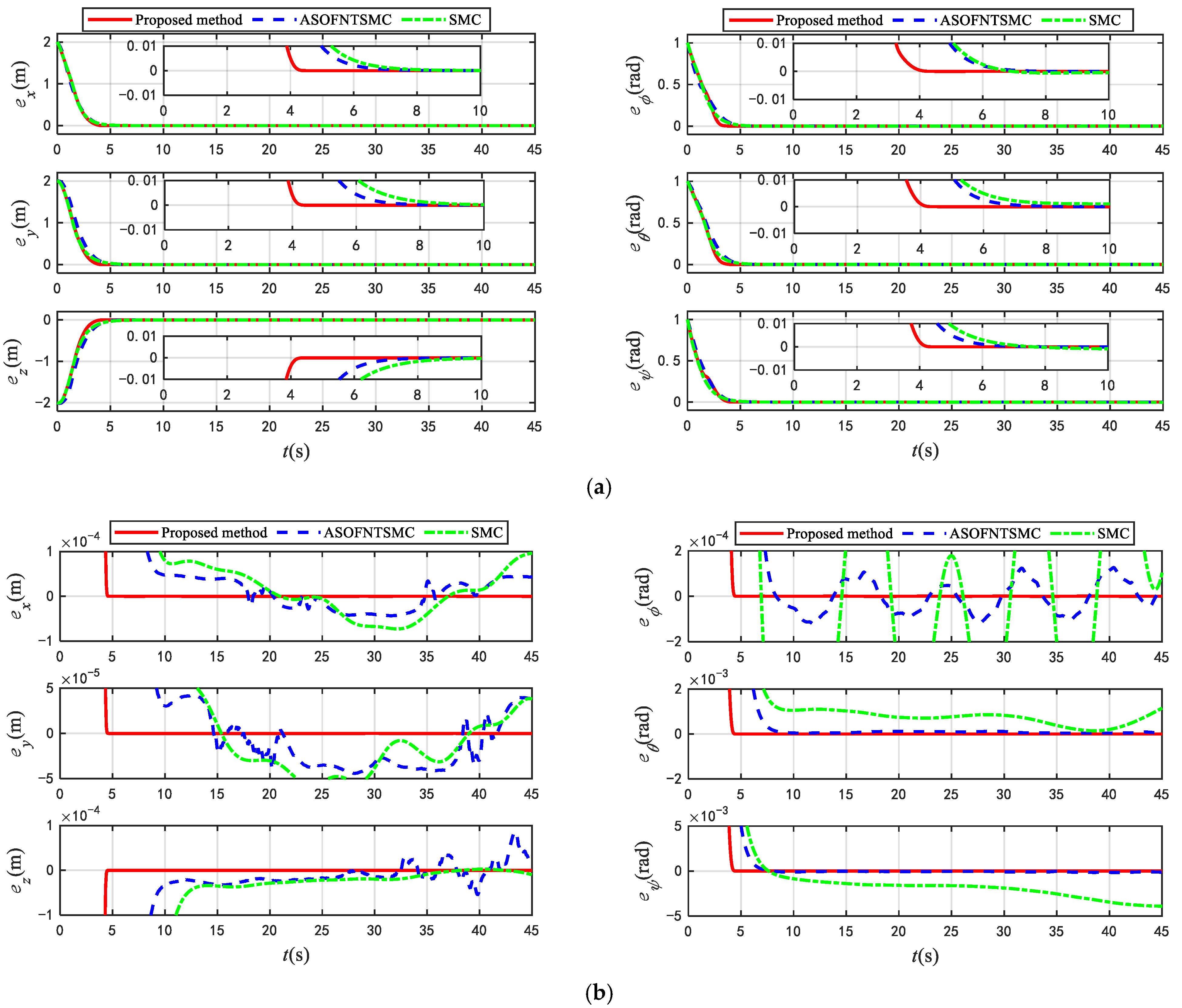
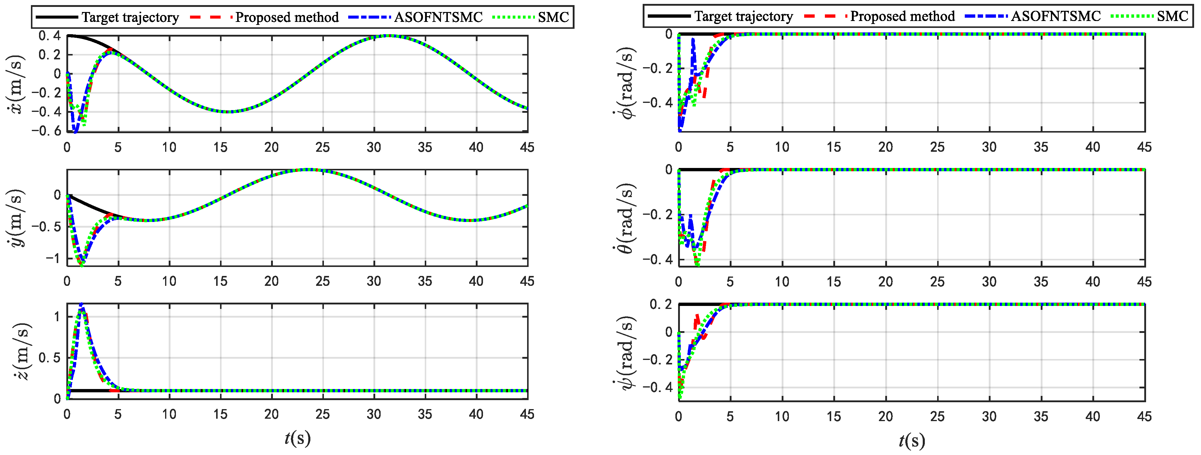
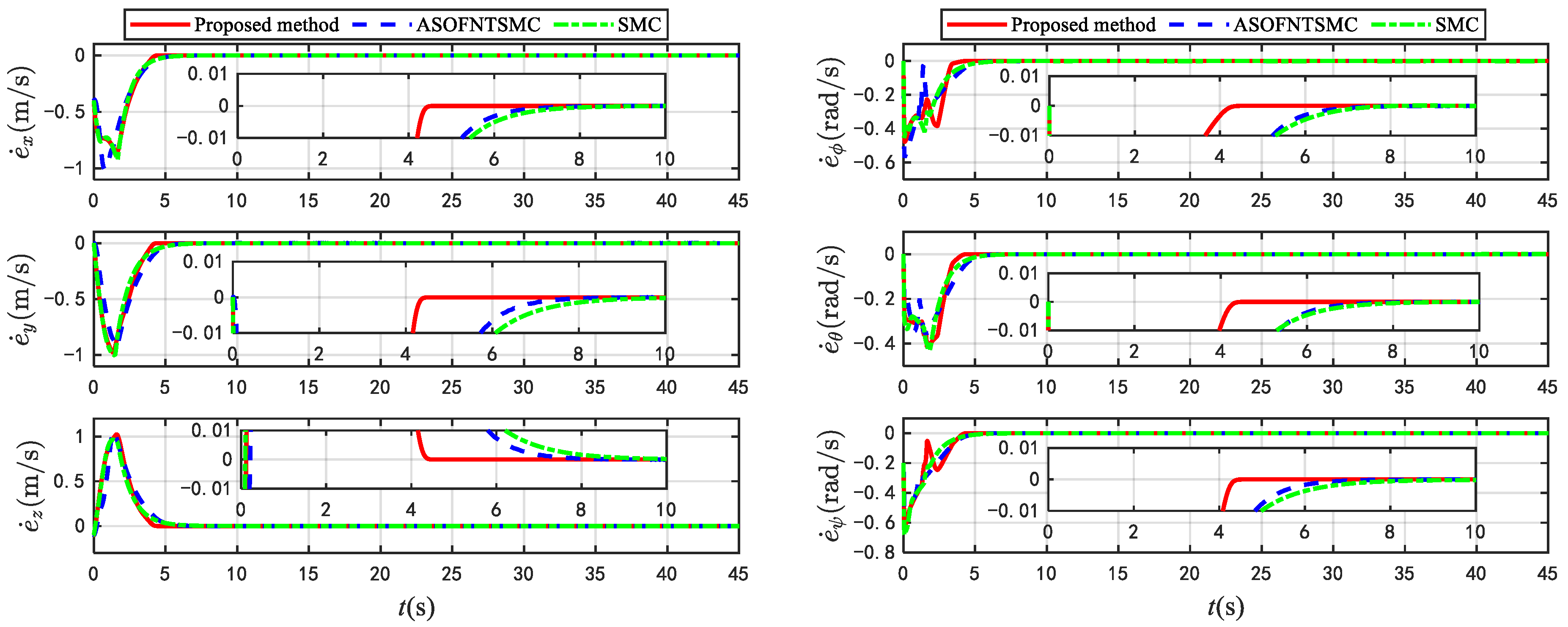
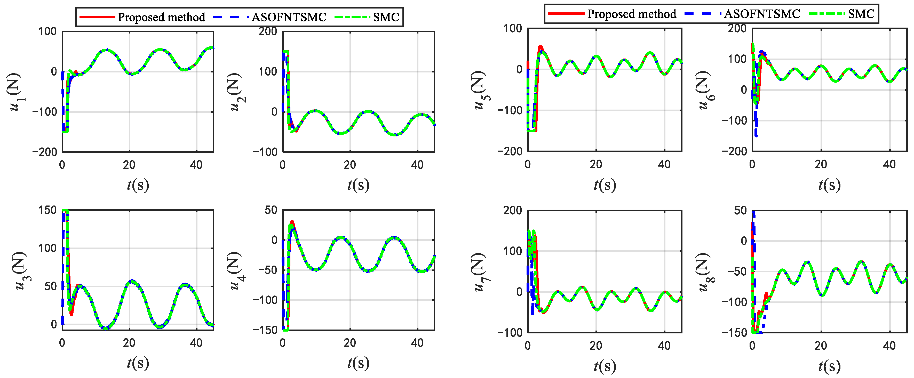
4. Simulation Verification

For the purpose of validating numerical tests of the controller, we conducted 3D trajectory tracking numerical simulations on an autonomous underwater vehicle model designed by the University of Hawaii. In addition, the introduced controller was contrasted with ordinary SMC [8] and ASOFNTSMC [41] for the objective evaluation of its tracking performance.

The simulation experiments were performed in MATLAB 2024b on a PC equipped with a 12th Gen Intel(R) Core(TM) i9-12900H (2.90 GHz) CPU. A fixed step-size of 0.01 s was used for all compared methods to ensure a consistent and fair comparison.

Noting that the employed spherical AUV is equipped with four thrusters both horizontally and vertically, based on the thruster distribution matrix $B_{\xi }$, the relationship between the nominal thrust vector ${\tau }_{\xi }={[{\tau }_u,{\tau }_v,{\tau }_w,{\tau }_p,{\tau }_q,{\tau }_r]}^T$ and the actuator input vector $u_{\xi }={[u_1,u_2,u_3,u_4,u_5,u_6,u_7,u_8]}^T$ can be given as [65]

$$u_{\xi }=B_{\xi }^T{(B_{\xi }{B}_{\xi }^T)}^{-1}{\tau }_{\xi }$$

(67)

where ${\tau }_{\xi }=J_A^T{\tau }_{\eta }$ is the command input vector and $B_{\xi }^T{(B_{\xi }{B}_{\xi }^T)}^{-1}$ denotes the pseudo-inverse matrix of $B_{\xi }$, with

$$B_{\xi }=\left[\begin{array}{llllllll}\overline{\varsigma }\hfill & -\overline{\varsigma }\hfill & -\overline{\varsigma }\hfill & \overline{\varsigma }\hfill & 0\hfill & 0\hfill & 0\hfill & 0\hfill \\ \overline{\varsigma }\hfill & \overline{\varsigma }\hfill & -\overline{\varsigma }\hfill & -\overline{\varsigma }\hfill & 0\hfill & 0\hfill & 0\hfill & 0\hfill \\ 0\hfill & 0\hfill & 0\hfill & 0\hfill & -1\hfill & -1\hfill & -1\hfill & -1\hfill \\ 0\hfill & 0\hfill & 0\hfill & 0\hfill & \overline{\varsigma }{R}_{\xi }\hfill & \overline{\varsigma }{R}_{\xi }\hfill & -\overline{\varsigma }{R}_{\xi }\hfill & -\overline{\varsigma }{R}_{\xi }\hfill \\ 0\hfill & 0\hfill & 0\hfill & 0\hfill & \overline{\varsigma }{R}_{\xi }\hfill & -\overline{\varsigma }{R}_{\xi }\hfill & -\overline{\varsigma }{R}_{\xi }\hfill & \overline{\varsigma }{R}_{\xi }\hfill \\ R_h\hfill & -R_h\hfill & R_h\hfill & -R_h\hfill & 0\hfill & 0\hfill & 0\hfill & 0\hfill \end{array}\right]$$

(68)

where $\overline{\varsigma }=\sin (0.25\pi )$, $R_{\xi }=0.381$ m, and $R_h=0.508$ m are constants associated with the model.

For the simulation experiments, the following model parameters are borrowed from [41], and the parametric uncertainties are modeled as 20% deviations from their nominal values. In terms of dynamics, the motion trajectory of AUV exhibits time-varying properties and is representable as a summation of parameter-varying sinusoidal signals. Thus, the reference targets are assumed to be

$$\left\{\begin{array}{l}{x}_d(t)=2\sin (t/5)m\hfill \\ y_d(t)=2\cos (t/5)m\hfill \\ z_d(t)=0.1t+3m\hfill \\ {\alpha }_d(t)=0rad\hfill \\ {\beta }_d(t)=-0.4rad\hfill \\ {\gamma }_d(t)=0.2trad\hfill \end{array}\right.$$

(69)

The marine environment is slow-time-varying and can be equated to the form of a superposition of a set of sinusoidal signals with diverse parameters [66]. Therefore, the external perturbations are chosen as

$$\left\{\begin{array}{l}{\tau }_{d\xi 1}=2\sin \left({\displaystyle \frac{t}{5}}+1\right)+4\cos \left({\displaystyle \frac{3t}{10}}+2\right)+5\sin \left({\displaystyle \frac{t}{10}}+3\right)N\hfill \\ {\tau }_{d\xi 2}=4\sin \left({\displaystyle \frac{t}{10}}+3\right)+5\cos \left({\displaystyle \frac{3t}{10}}+3\right)+3\sin \left({\displaystyle \frac{t}{5}}+4\right)N\hfill \\ {\tau }_{d\xi 3}=2\sin \left({\displaystyle \frac{t}{5}}+4\right)+3\cos \left({\displaystyle \frac{t}{10}}+5\right)+2\sin \left({\displaystyle \frac{t}{5}}+3\right)N\hfill \\ {\tau }_{d\xi 4}=5\sin \left({\displaystyle \frac{t}{10}}+2\right)+2\cos \left({\displaystyle \frac{2t}{5}}+3\right)+3\sin \left({\displaystyle \frac{t}{5}}+2\right)N\cdot m\hfill \\ {\tau }_{d\xi 5}=2\sin \left({\displaystyle \frac{3t}{10}}+2\right)+3\cos \left({\displaystyle \frac{t}{5}}+6\right)+\sin \left({\displaystyle \frac{3t}{10}}+3\right)N\cdot m\hfill \\ {\tau }_{d\xi 6}=3\sin \left({\displaystyle \frac{t}{5}}+5\right)+5\cos \left({\displaystyle \frac{t}{10}}+3\right)+4\sin \left({\displaystyle \frac{t}{10}}+3\right)N\cdot m\hfill \end{array}\right.$$

(70)

During experimental comparisons, the initial states are assigned as $\eta (0)=[2,4,1,$$1,0.6,1{]}^T$ and $\xi (0)={[0,0,0,0,0,0]}^T$. It should be emphasized that to maintain fairness during performance comparison, the parameters are selected on the principle of ensuring that the different control methods consume almost the same amount of energy $(E_u=‖{\displaystyle {\int }_0^{45}\left|u_{\xi }\right|dt}‖)$. As shown in Figure 4, the suggested control strategy requires slightly less actuation energy than the remaining two methods, so it can be ensured that the simulation experiment represents an impartial comparison of different approaches’ performance in the context of the same energy consumption.

Table 2. Controller design parameters for the three control schemes.

Control Scheme	Parameter
SMC	$\begin{array}{l}{K}_{v1}=diag(1.2,1,1),K_{v2}=[1,0,0;0,1.1,0;0,0,1]\\ K=diag(2,2,2,2,2,2)\\ \beta =diag(20,20,20,20,20,20)\end{array}$
ASOFNTSMC	$\begin{array}{l}b=3,b=3,g=11,h=3,{\phi }_i=0.1\\ K_1=diag(1.5,1.5,1.5,1.5,1.5,1.5)\\ K_2=diag(1,1,1,1,1,1)\\ K_3=diag(1.5,1.5,1.5,2.5,2,2)\end{array}$
Proposed method	$\begin{array}{l}\iota =1,{\lambda }_2=1,{\lambda }_3=2,{\varpi }_0=0.5,{\rho }_0=0.01,l_0={10}^4,l_1=0.9,l_2=0.1,\epsilon =0.01\\ k_1=0.5,f(0)=\varpi (0)=\overline{\varphi }(0)=\widehat{\delta }(0)=0\\ \widehat{\Theta }(0)=0\in {ℝ}^{6\times 1},T_{ai}=T_{bi}=T_{ci}=5.5,{\vartheta }_{ax}=0.8,{\vartheta }_{ay}={\vartheta }_{az}=1\\ {\vartheta }_{a\alpha }={\vartheta }_{a\beta }={\vartheta }_{a\gamma }=0.5,{\vartheta }_{bx}=3,{\vartheta }_{by}={\vartheta }_{bz}={\vartheta }_{b\alpha }={\vartheta }_{b\beta }={\vartheta }_{b\gamma }=2.5\\ {\sigma }_{ai}=0.01,{\sigma }_{bi}=0.2(i=x,y,z,\alpha ,\beta ,\gamma ),K_1=diag=(1,1,1,1,1,1)\\ K_2=diag(0.1,0.1,0.1,0.1,0.1,0.1),K_3=diag(0.1,0.1,0.1,0.1,0.1,0.1)\end{array}$

presents the design parameters.

Figure 5 demonstrates that the closed-loop AUV system successfully tracks the spiral trajectory under all three control schemes, but based on the local zoomed view, it demonstrates that the proposed method h achieves a shorter settling time to approximate the target trajectory. From Figure 6, we can see the estimated lumped disturbance converges rapidly to its actual value in a short period of time.

In this section, the steady-state maximum allowable errors for position tracking error $(e_x,e_y,e_z)$ and attitude tracking error $(e_{\alpha },e_{\beta },e_{\gamma })$ are 0.01 m and 0.01 rad, respectively. From Figure 7, we can see the tracking effect of position and attitude is high-precision.

From Figure 8a, the SMC control strategy exhibited higher exponential convergence rate when the error was large; however, when the tracking error approached the steady state, the convergence rate of the SMC was greatly reduced. The ASOFNTSMC control method improved the convergence speed as the error approached the equilibrium point, but the settling time achieved by the suggested algorithm was significantly one second less than it. Figure 8b shows that the introduced method exhibited superior tracking accuracy compared to ASOFNTSMC and SMC; theoretical analysis confirms that it ensures a predefined bounded region $(\left|e_i\right|<{10}^{-6}m\mathrm{for}\mathrm{t}>3.9\mathrm{s})$ is where the tracking error converges, whereas the errors generated by the comparative methods remain within a larger interval $B_1=\{\left|e_i\right|<1\times {10}^{–4},t>5.5s\}$ for ASOFNTSMC and $B_2=\{\left|e_i\right|<5\times {10}^{–3},$ $t>6.2s\}$ for SMC. Combining Figure 9 and Figure 10 demonstrates that the derivative of the tracking error also has accelerated convergence with superior steady-state accuracy. Similarly, Figure 8 and Figure 10 show that the proposed strategy effectively increases the closed-loop system exponential convergence without causing overshoot. According to Figure 11, the actual actuator inputs of the proposed method do not produce significant chattering.

According to the experimental findings and analysis presented, we can infer that the designed control strategy outperformed the SMC and ASOFNTSMC methods with respect to response speed and transient accuracy, while consuming the same amount of energy.

5. Conclusions

5.1. The Main Work

In this study, a prescribed-performance sliding-mode control scheme was developed for AUV trajectory tracking under model uncertainty and oceanic disturbances, which ensures that the trajectory tracking errors and their rates of change are suppressed within the preset ranges after the specified time. The designed AFTSMDO is independent of the upper bound of the perturbations. And the designed control strategy has the following advantages based on the simulation results:

(1)

Parameters are not constrained by the initial conditions;

(2)

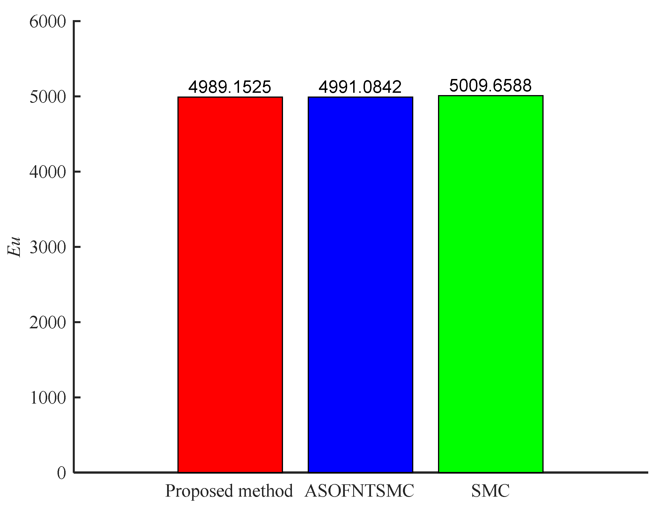
The developed control approach effectively improves the convergence rate and tracking accuracy of the system without sacrificing a significant amount of energy.

5.2. Future Work

The developed control strategy failed to account for the cases where the system may have deviated from the prescribed performance due to factors such as actuator failures or sudden external perturbations.

Future research will focus on algorithmic optimization and the integration of a safety margin into the prescribed performance function, validated via physical AUV prototyping.

References

1. Hu, X.; Wei, X.; Kao, Y.; Han, J. Robust Synchronization for Under-Actuated Vessels Based on Disturbance Observer. IEEE Trans. Intell. Transp. Syst. 2022, 23, 5470–5479. [Google Scholar] [CrossRef]
2. Hu, X.; Zhu, G.; Ma, Y.; Li, Z.; Malekian, R.; Sotelo, M.A. Dynamic Event-Triggered Adaptive Formation with Disturbance Rejection for Marine Vehicles Under Unknown Model Dynamics. IEEE Trans. Veh. Technol. 2023, 72, 5664–5676. [Google Scholar] [CrossRef]
3. Peng, Z.; Wang, J.; Wang, J. Constrained Control of Autonomous Underwater Vehicles Based on Command Optimization and Disturbance Estimation. IEEE Trans. Ind. Electron. 2019, 66, 3627–3635. [Google Scholar] [CrossRef]
4. Liang, X.; Li, Y.; Peng, Z.; Zhang, J. Nonlinear dynamics modeling and performance prediction for underactuated AUV with fins. Nonlinear Dyn. 2016, 84, 237–249. [Google Scholar] [CrossRef]
5. Yan, Z.; Yu, H.; Hou, S. Diving control of underactuated unmanned undersea vehicle using integral-fast terminal sliding mode control. J. Cent. South Univ. 2016, 23, 1085–1094. [Google Scholar] [CrossRef]
6. Elhaki, O.; Shojaei, K. A robust neural network approximation-based prescribed performance output-feedback controller for autonomous underwater vehicles with actuators saturation. Engineering Applications of Artificial Intelligence 2020, 88. [Google Scholar] [CrossRef]
7. Utkin, V.I. Sliding Modes in Control and Optimization; Springer: Berlin/Heidelberg, Germany, 1992. [Google Scholar]
8. Yang, Y.C.; Yang, K.S.; Chen, C.Y.; Mu, L.J.; Yang, W.C. Robust trajectory control for an autonomous underwater vehicle. In Proceedings of the 2013 MTS/IEEE OCEANS, Bergen, Norway, 10–14 June 2013; IEEE: Piscataway, NJ, USA, 2013. [Google Scholar]
9. Jiang, Y.; Guo, C.; Yu, H. Robust trajectory tracking control for an underactuated autonomous underwater vehicle based on bioinspired neurodynamics. International Journal of Advanced Robotic Systems 2018, 15. [Google Scholar] [CrossRef]
10. Karkoub, M.; Wu, H.M.; Hwang, C.L. Nonlinear trajectory-tracking control of an autonomous underwater vehicle. Ocean Eng. 2017, 145, 188–198. [Google Scholar] [CrossRef]
11. Yan, Z.; Wang, M.; Xu, J. Robust adaptive sliding mode control of underactuated autonomous underwater vehicles with uncertain dynamics. Ocean Eng. 2019, 173, 802–809. [Google Scholar] [CrossRef]
12. Cristi, R.; Papoulias, F.A. Adaptive Sliding Mode Control of Autonomous Underwater Vehicles in the Dive Plane. IEEE J. Ocean. Eng. 1990, 15, 152–160. [Google Scholar] [CrossRef]
13. Lee, D.; Kim, H.J.; Sastry, S. Feedback linearization vs. adaptive sliding mode control for a quadrotor helicopter. Int. J. Control Autom. Syst. 2009, 7, 419–428. [Google Scholar] [CrossRef]
14. Elmokadem, T.; Zribi, M.; Youcef-Toumi, K. Terminal sliding mode control for the trajectory tracking of underactuated Autonomous Underwater Vehicles. Ocean Eng. 2017, 129, 613–625. [Google Scholar] [CrossRef]
15. Zhihong, M.; Yu, X.H. Terminal sliding mode control of MIMO linear systems. IEEE Trans. Circuits Syst. I Fundam. Theory Appl. 2002, 44, 1065–1070. [Google Scholar] [CrossRef]
16. Yu, X.; Feng, Y.; Man, Z. Terminal sliding mode control—An overview. IEEE Open J. Ind. Electron. Soc. 2020, 2, 36–52. [Google Scholar] [CrossRef]
17. Tang, Y. Terminal sliding mode control for rigid robots. Automatica 1998, 34, 51–56. [Google Scholar] [CrossRef]
18. Mobayen, S. An adaptive fast terminal sliding mode control combined with global sliding mode scheme for tracking control of uncertain nonlinear third-order systems. Nonlinear Dyn. 2015, 82, 599–610. [Google Scholar] [CrossRef]
19. Feng, Y.; Yu, X.; Man, Z. Non-singular terminal sliding mode control of rigid manipulators. Automatica 2002, 38, 2159–2167. [Google Scholar] [CrossRef]
20. Rangel, M.A.G.; Manzanilla, A.; Suarez, A.E.Z.; Muoz, F.; Lozano, R. Adaptive Non-singular Terminal Sliding Mode Control for an Unmanned Underwater Vehicle: Real-time Experiments. Int. J. Control Autom. Syst. 2020, 18, 615–628. [Google Scholar] [CrossRef]
21. Komurcugil, H. Non-singular terminal sliding-mode control of DC–DC buck converters. Control Eng. Pract. 2013, 21, 321–332. [Google Scholar] [CrossRef]
22. Truong, T.N.; Vo, A.T.; Kang, H.-J. A backstepping global fast terminal sliding mode control for trajectory tracking control of industrial robotic manipulators. IEEE Access 2021, 9, 31921–31931. [Google Scholar] [CrossRef]
23. Yu, X.; Zhihong, M. Fast terminal sliding-mode control design for nonlinear dynamical systems. IEEE Trans. Circuits Syst. I Fundam. Theory Appl. 2009, 49, 261–264. [Google Scholar]
24. Boukattaya, M.; Mezghani, N.; Damak, T. Adaptive nonsingular fast terminal sliding-mode control for the tracking problem of uncertain dynamical systems. ISA Trans. 2018, 77, 1–19. [Google Scholar] [CrossRef] [PubMed]
25. Yang, L.; Yang, J. Nonsingular fast terminal sliding-mode control for nonlinear dynamical systems. Int. J. Robust Nonlinear Control 2011, 21, 1865–1879. [Google Scholar] [CrossRef]
26. Wang, Y.; Zhu, K.; Chen, B.; Jin, M. Model-free continuous nonsingular fast terminal sliding mode control for cable-driven manipulators. ISA Trans. 2020, 98, 483–495. [Google Scholar] [CrossRef]
27. Xu, B.; Zhang, L.; Ji, W. Improved non-singular fast terminal sliding mode control with disturbance observer for PMSM drives. IEEE Trans. Transp. Electrif. 2021, 7, 2753–2762. [Google Scholar] [CrossRef]
28. Song, Z.; Sun, K. Prescribed performance tracking control for a class of nonlinear system considering input and state constraints. ISA Trans. 2022, 119, 81–92. [Google Scholar] [CrossRef]
29. Song, Z.; Liu, J.; Sun, K. Performance-guaranteed fault tolerant control for Euler-Lagrange systems with actuator faults and uncertain disturbance. Proc. Inst. Mech. Eng. Part I-J. Syst. Control. Eng. 09596518251322239. [CrossRef]
30. Song, Z.; Sun, K. Adaptive fault tolerant control for a small coaxial rotor unmanned aerial vehicles with partial loss of actuator effectiveness. Aerospace Science and Technology 2019, 88, 362–379. [Google Scholar] [CrossRef]
31. Li, J.; Du, J.; Sun, Y.; Lewis, F.L. Robust adaptive trajectory tracking control of underactuated autonomous underwater vehicles with prescribed performance. Int. J. Robust Nonlinear Control. 2019, 29, 4629–4643. [Google Scholar] [CrossRef]
32. Sun, H.; Zong, G.; Cui, J.; Shi, K. Fixed-time sliding mode output feedback tracking control for autonomous underwater vehicle with prescribed performance constraint. Ocean Eng. 2022, 247, 110673. [Google Scholar] [CrossRef]
33. Rong, S.; Wang, H.; Li, H.; Sun, W.; Gu, Q.; Lei, J. Performance-guaranteed fractional-order sliding mode control for underactuated autonomous underwater vehicle trajectory tracking with a disturbance observer. Ocean Eng. 2022, 263, 112330. [Google Scholar] [CrossRef]
34. Wang, H.; Bai, W.; Zhao, X.; Liu, P.X. Finite-time-prescribed performance-based adaptive fuzzy control for strict-feedback nonlinear systems with dynamic uncertainty and actuator faults. IEEE Trans. Cybern. 2021, 52, 6959–6971. [Google Scholar] [CrossRef] [PubMed]
35. Li, J.; Du, J.; Chen, C.P. Command-filtered robust adaptive NN control with the prescribed performance for the 3-D trajectory tracking of underactuated AUVs. IEEE Trans. Neural Netw. Learn. Syst. 2021, 33, 6545–6557. [Google Scholar] [CrossRef] [PubMed]
36. Wang, C.; Zhu, S.; Yu, W.; Song, L.; Guan, X. Adaptive prescribed performance control of nonlinear asymmetric input saturated systems with application to AUVs. J. Frankl. Inst. 2021, 358, 8330–8355. [Google Scholar] [CrossRef]
37. Zhou, S.; Song, Y.; Luo, X. Fault-tolerant tracking control with guaranteed performance for nonlinearly parameterized systems under uncertain initial conditions. J. Frankl. Inst. 2020, 357, 6805–6823. [Google Scholar] [CrossRef]
38. Fossen, T.I. Handbook of Marine Craft Hydrodynamics and Motion Control; John Wiley & Sons: Hoboken, NJ, USA, 2011. [Google Scholar]
39. Liu, H.; Qi, Z.; Yuan, J.; Tian, X. Robust fixed-time H∞ tracking control of UUVs with partial and full state constraints and prescribed performance under input saturation. Ocean Eng. 2023, 283, 115023. [Google Scholar] [CrossRef]
40. Zhang, M.; Liu, X.; Yin, B.; Liu, W. Adaptive terminal sliding mode based thruster fault tolerant control for underwater vehicle in time-varying ocean currents. J. Frankl. Inst. 2015, 352, 4935–4961. [Google Scholar] [CrossRef]
41. Qiao, L.; Zhang, W. Adaptive second-order fast nonsingular terminal sliding mode tracking control for fully actuated autonomous underwater vehicles. IEEE J. Ocean. Eng. 2018, 44, 363–385. [Google Scholar] [CrossRef]
42. Wan, L.; Cao, Y.; Sun, Y.; Qin, H. Fault-tolerant trajectory tracking control for unmanned surface vehicle with actuator faults based on a fast fixed-time system. ISA Trans. 2022, 130, 79–91. [Google Scholar] [CrossRef]
43. An, S.; Wang, L.; He, Y. Robust fixed-time tracking control for underactuated AUVs based on fixed-time disturbance observer. Ocean Eng. 2022, 266, 112567. [Google Scholar] [CrossRef]
44. Bhat, S.P.; Bernstein, D.S. Finite-time stability of continuous autonomous systems. SIAM J. Control Optim. 2000, 38, 751–766. [Google Scholar] [CrossRef]
45. Hu, Q.; Li, B.; Qi, J. Disturbance observer based finite-time attitude control for rigid spacecraft under input saturation. Aerosp. Sci. Technol. 2014, 39, 13–21. [Google Scholar] [CrossRef]
46. Zhou, S.; Wang, X.; Song, Y. Prescribed performance tracking control under uncertain initial conditions: A neuroadaptive output feedback approach. IEEE Trans. Cybern. 2022, 53, 7213–7223. [Google Scholar] [CrossRef]
47. Song, Z.; Sun, K. Prescribed performance adaptive control for an uncertain robotic manipulator with input compensation updating law. J. Frankl. Inst. 2021, 358, 8396–8418. [Google Scholar] [CrossRef]
48. Zhu, Y.; Qiao, J.; Guo, L. Adaptive sliding mode disturbance observer-based composite control with prescribed performance of space manipulators for target capturing. IEEE Trans. Ind. Electron. 2018, 66, 1973–1983. [Google Scholar] [CrossRef]
49. Li, J.; Du, J. Adaptive disturbance cancellation for a class of MIMO nonlinear Euler–Lagrange systems under input saturation. ISA Trans. 2020, 96, 14–23. [Google Scholar] [CrossRef]
50. Sun, T.; Cheng, L.; Wang, W.; Pan, Y. Semiglobal exponential control of Euler-Lagrange systems using a sliding-mode disturbance observer. Automatica 2020, 112, 108677. [Google Scholar] [CrossRef]
51. Shao, K.; Zheng, J.; Wang, H.; Xu, F.; Wang, X.; Liang, B. Recursive sliding mode control with adaptive disturbance observer for a linear motor positioner. Mech. Syst. Signal Process. 2021, 146, 107014. [Google Scholar] [CrossRef]
52. Edwards, C.; Shtessel, Y.B. Adaptive continuous higher order sliding mode control. Automatica 2016, 65, 183–190. [Google Scholar] [CrossRef]
53. Chen, W.H.; Ballance, D.J. A nonlinear disturbance observer for robotic manipulators. IEEE Trans. Ind. Electron. 2000, 47, 932–938. [Google Scholar] [CrossRef]
54. Nguyen, Q.D.; Huang, S.-C.; Giap, V.N. Lyapunov-based fractional order of disturbance observer and sliding mode control for a secure communication of chaos-based system. Int. J. Control Autom. Syst. 2023, 21, 3595–3606. [Google Scholar] [CrossRef]
55. Giap, V.N.; Nguyen, Q.D.; Trung, N.K.; Huang, S.-C. Time-varying disturbance observer based on sliding-mode observer and double phases fixed-time sliding mode control for a TS fuzzy micro-electro-mechanical system gyroscope. J. Vib. Control 2023, 29, 1927–1942. [Google Scholar] [CrossRef]
56. Hwang, S.; Kim, H.S. Extended Disturbance Observer-Based Integral Sliding Mode Control for Nonlinear System via T-S Fuzzy Model. IEEE Access 2020, 8, 116090–116105. [Google Scholar] [CrossRef]
57. Kumar, T.R.D.; Mija, S.J. Boundary Logic-Based Hybrid PID-SMC Scheme for a Class of Underactuated Nonlinear Systems-Design and Real-Time Testing. IEEE Trans. Ind. Electron. 2025, 72, 5257–5267. [Google Scholar] [CrossRef]
58. Pal, P.; Behera, R.K.; Muduli, U.R. Eliminating Current Sensor Dependencies in DAB Converters Using a Luenberger Observer-Based Hybrid Approach. IEEE Trans. Ind. Appl. 2024, 60, 6380–6392. [Google Scholar] [CrossRef]
59. Zhang, X.; Lu, Z.; Yuan, X.; Wang, Y.; Shen, X. L2-Gain Adaptive Robust Control for Hybrid Energy Storage System in Electric Vehicles. IEEE Trans. Power Electron. 2021, 36, 7319–7332. [Google Scholar] [CrossRef]
60. Karahan, O.; Karci, H. Design of robust fractional order fuzzy PID sliding mode controller based on hybrid swarm intelligence algorithm for a 6-DOF robotic manipulator. Robotica 2025, 43, 1110–1139. [Google Scholar] [CrossRef]
61. Ma, Y.; He, L.; Song, T.; Wang, D. Adaptive path-tracking control with passivity-based observer by port-Hamiltonian model for autonomous vehicles. IEEE Trans. Intell. Veh. 2023, 8, 4120–4130. [Google Scholar] [CrossRef]
62. Chabukswar, A.; Wandhare, R. Modified Back-Stepping Sliding Mode Controller with Robust Observer-Less Disturbance Rejection for DC Microgrid Applications. IEEE Trans. Power Electron. 2025, 40, 451–466. [Google Scholar] [CrossRef]
63. Fu, B.; Che, W.; Wang, Q.; Liu, Y.; Yu, H. Improved sliding-mode control for a class of disturbed systems based on a disturbance observer. J. Frankl. Inst. 2024, 361, 106699. [Google Scholar] [CrossRef]
64. Zhang, L.; Liu, X.; Zong, G.; Wang, W. Kalman filter-based SMC for systems with noise and disturbances: Applications to magnetic levitation system. Int. J. Syst. Sci. 2025. [Google Scholar] [CrossRef]
65. Qiao, L.; Zhang, W. Adaptive non-singular integral terminal sliding mode tracking control for autonomous underwater vehicles. IET Control Theory Appl. 2017, 11, 1293–1306. [Google Scholar] [CrossRef]
66. Li, J.; Du, J.; Hu, X. Robust adaptive prescribed performance control for dynamic positioning of ships under unknown disturbances and input constraints. Ocean Eng. 2020, 206, 107254. [Google Scholar] [CrossRef]
Figure 1. The integrated architecture of the proposed strategy.
Jmse 13 01252 g001
Figure 2. Visualization of Ω R 1 and Ω R 2 .
Jmse 13 01252 g002
Figure 3. Tracking error and its derivative curves independent of initial conditions.
Jmse 13 01252 g003
Figure 4. Histogram of the energy consumption for the three methods.
Jmse 13 01252 g004
Figure 5. Trajectory tracking performance curves (a) in 3D space; and (b) in the x–y plane.
Jmse 13 01252 g005
Figure 6. Comprehensive disturbance estimation performance of the designed AFTSMDO.
Jmse 13 01252 g006
Figure 7. Position and attitude tracking curves.
Jmse 13 01252 g007
Figure 8. (a) Position tracking errors and attitude tracking error curves. (b) Localized magnification of tracking errors.
Jmse 13 01252 g008
Figure 9. Linear and angular velocity tracking curves.
Jmse 13 01252 g009
Figure 10. The derivative curves of the tracking errors.
Jmse 13 01252 g010
Figure 11. Thrust curves of the thrusters.
Jmse 13 01252 g011