Dispersion Mechanism and Sensitivity Analysis of Coral Sand

Abstract

A lime–sand island–reef formation has a dual structure consisting of an overlying loose or weakly consolidated coral sand (CS) layer and an underlying reef limestone layer. The coral sand layer is the sole carrier of the underground freshwater lens in the lime–sand island–reef, and it differs in terms of its hydraulic properties from common terrigenous quartz sand (QS). This study investigated the mechanism of freshwater lens formation, dominated by solute dispersion, combining multi-scale experiments and numerical simulations (GMS) to reveal the control mechanisms behind the dispersion properties of coral sand and their role in freshwater lens formation. Firstly, the dispersion test and microscopic characterization revealed the key differences in coral sand in terms of its roundness, roughness, particle charge, and surface hydrophilicity. Accordingly, a hierarchical conversion model for the coral sand–quartz sand coefficient of dispersion (COD) was established (R² > 0.99). Further, combining this with numerical simulation in GMS revealed that the response pattern of the coefficient of dispersion to key parameters of freshwater lens development is as follows: freshwater appearance time > steady-state freshwater body thickness > steady-state freshwater reserve > lens stabilization time. These results clarify the development mechanism and formation process behind freshwater lenses on island reefs, from the micro to the macro scale, and provide a scientific basis for optimizing the protection of freshwater resources in coral islands and guiding the construction of artificial islands.

1. Introduction

A large number of natural and artificially created gray sand islands are distributed throughout the South China Sea [1], and they play a crucial role in the development of China’s marine resources [1]. Unlike reclamation projects along the mainland coast, the gray sand islands in the South China Sea have a typical binary geological structure, with Holocene unconsolidated or weakly consolidated coral clasts on the surface and Pleistocene rock-forming reef tuffs in the lower layer [2,3]. Since most of these islands are far from the mainland and lack surface water resources, underground freshwater is essential for supporting islanders’ lives and maintaining ecological nourishment [4,5]. The freshwater on gray sand islands is rainfall that infiltrates the coral sand (CS) aquifer. Due to density differences, freshwater is suspended in seawater in the middle and at the sides, forming what is known as a “freshwater lens” [6,7]. In the South China Sea, coral sand is the only carrier of the freshwater lens [4,8], and its hydrological properties significantly impact the formation and storage of the freshwater lens.

Coral sand is a special soil of marine origin [8,9] with special particle morphology and structural characteristics. These features are due to its material sources (e.g., corals, shells, algae, and other remains of marine organisms) and action processes (e.g., oceanic erosion, transport, and accumulation) [10,11]. Studies have shown that coral sand contains more than 90% calcium carbonate [12], has a porous and irregular morphology [13], and breaks easily [14]. These properties differ significantly from those of quartz sand of terrestrial origin. Therefore, studying the hydrophysical properties of coral sand and its role in the formation and evolution of freshwater lenses is crucial to maintaining the stability of our national and international islands and safeguarding the freshwater supply to island residents. The formation and evolution of freshwater lenses often take decades, which makes them difficult to replicate through conventional physical experiments. Thus, numerical simulation has become a common means of studying these freshwater lenses [15,16,17,18,19]. In numerical simulations, accurately setting the stratigraphic information, boundary conditions, and initial conditions is crucial to accurately representing the real situation. Stratigraphic information includes stratigraphic stratification and hydrogeological parameters [7]. The former can be obtained through hydrological boreholes or physical exploration. However, determining the latter is more difficult. Currently, the most common methods for obtaining hydrogeological parameters are the on-site pumping test [18] and the tidal water level inversion method [19]. The pumping test is usually not recommended for use on islands and reefs because extracting a large amount of groundwater will damage the underground freshwater lens of the reef. The tidal inversion method requires extensive tidal observation data and a longer test period, making it more costly. For this reason, indoor experimental techniques have been widely used to obtain the key hydrogeological parameters (e.g., permeability and dispersion coefficients) for coral sand strata and apply them to numerical simulations to study the formation and evolution mechanisms for freshwater lenses on coral islands [15,16,17,20].

In gray sand islands, the formation of freshwater lenses involves the convection and dispersion of groundwater to reach a steady state. Therefore, studying the characteristics of solute dispersion within coral sand is essential for revealing the formation and evolution mechanisms in freshwater lenses. Many previous researchers have studied this topic [21,22,23,24,25,26,27,28,29]. In the earliest instance, Taylor [28] proposed a method for calculating the longitudinal coefficient of dispersion (COD) in porous media that considered only convection. He also provided a formula that related the longitudinal COD to the molecular COD. Zhang et al. [27] gave specific formulas and test methods for calculating the CODs for four different water flows and initial salt concentrations. They derived a method for calculating the hydrodynamic COD based on the principle of mass conservation. Sahimi [25,26] studied the hydrodynamic dispersion problem in two types of heterogeneous porous media: one type in which some pores did not allow material transport and another type with a fractal distribution of permeability in each region of the pore space. Shi et al. [29] proposed the intercept method, an approximate method for estimating the convective dispersion formula (CDE) parameters, and verified it using experiments. This method can be widely used to calculate the parameters of the dispersion formulas for soil solute transport. Zhang et al. [24] established the relationship between the longitudinal COD and the variance in and scale of randomly distributed permeability coefficients. They analyzed this relationship in comparison to the results obtained using Gelhar’s theoretical calculations [30]. Jensen et al. [23] utilized the nonlinear least-squares optimization program developed by Parker and Vangenuchten [22] for curve fitting to obtain the parameter values for various convection–dispersion formulas. Cui et al. [21] divided dispersions into five types based on the relative weights of molecular diffusion and mechanical diffusion at various flow rates and provided the corresponding flow rate thresholds. Mahmoodlu et al. [31] investigated how the dispersion coefficient (COD) varied in saturated sand samples of four different grain sizes. Their experimental results showed that the COD mainly depends on particle size. Guo et al. [32] investigated the variation rule for the COD in unsaturated porous media. They developed a six-parameter empirical model to predict the effects of saturation and the Peclet number (the ratio of advective transport to diffusive transport) on the COD of unsaturated porous media. The above studies on dispersion have primarily focused on the methods for calculating the COD and parameter fitting, laying a foundation for theoretical research on dispersion.

Currently, domestic and international research on the solute diffusivity of porous media primarily focuses on terrestrial sand. There have been limited microscopic analyses of the diffusivity characteristics of coral sand (CS). This study uses quartz sand (QS) as a control group to systematically investigate the dispersion characteristics of coral sand. This analysis reveals the microscopic mechanisms underlying the differences in dispersion between CS and QS and proposes a conversion formula for their dispersion coefficients. Using the GMS (version 10.4) groundwater numerical simulation system, a sensitivity analysis was conducted on the response of the freshwater lens in coral reefs as the COD of coral sand was varied within a reasonable range. The analysis thoroughly explored the impact of changes in the diffusion characteristics on the formation and stability of the freshwater lens. This study enriches the theoretical framework for solute transport in CS, providing a scientific basis for the rational development and management of freshwater resources on islands and reefs. It also has potential applications in the construction of artificial islands and the sustainable utilization of freshwater resources.

2. The Study Area and Sample Characteristics

2.1. The Study Area

The study area is located on an island in the Xisha Islands of the South China Sea (Figure 1a) at a latitude of 16°59′ and a longitude of 112°16′. The island is a typical artificial island formed through land reclamation based on natural reefs. Based on stratigraphic information revealed through field drilling, the study area exhibits a typical two-layer hydrogeological structure. The upper layer consists of coral sand (CS), and the lower layer comprises reef limestone (Figure 1b). The interface between the CS layer and the underlying reef limestone layer is located 19–20 m below ground level and is known as the “Thurber Discontinuity” [33]. Given these stratigraphic structural characteristics, subsequent numerical simulations in this paper adopt the aforementioned two-layer aquifer structural model.

The coral sand (CS) layer primarily consists of gravelly sand with localized minor amounts of silt, medium sand, coarse sand, and angular gravel. The laboratory particle analysis of undisturbed coral sediment cores (Figure 1c) shows that the coefficient of uniformity ($C_{\mathrm{u}}$) is 25, and the coefficient of curvature ($C_{\mathrm{c}}$) is 0.36, according to the “Code for investigation of geotechnical engineering” (GB50021-2009) [34]. These values indicate that the sand layer has poor gradation. The results from in situ dynamic cone penetration tests (hammer energy: 63.5 kg) indicate that the CS layer is loose to slightly dense.

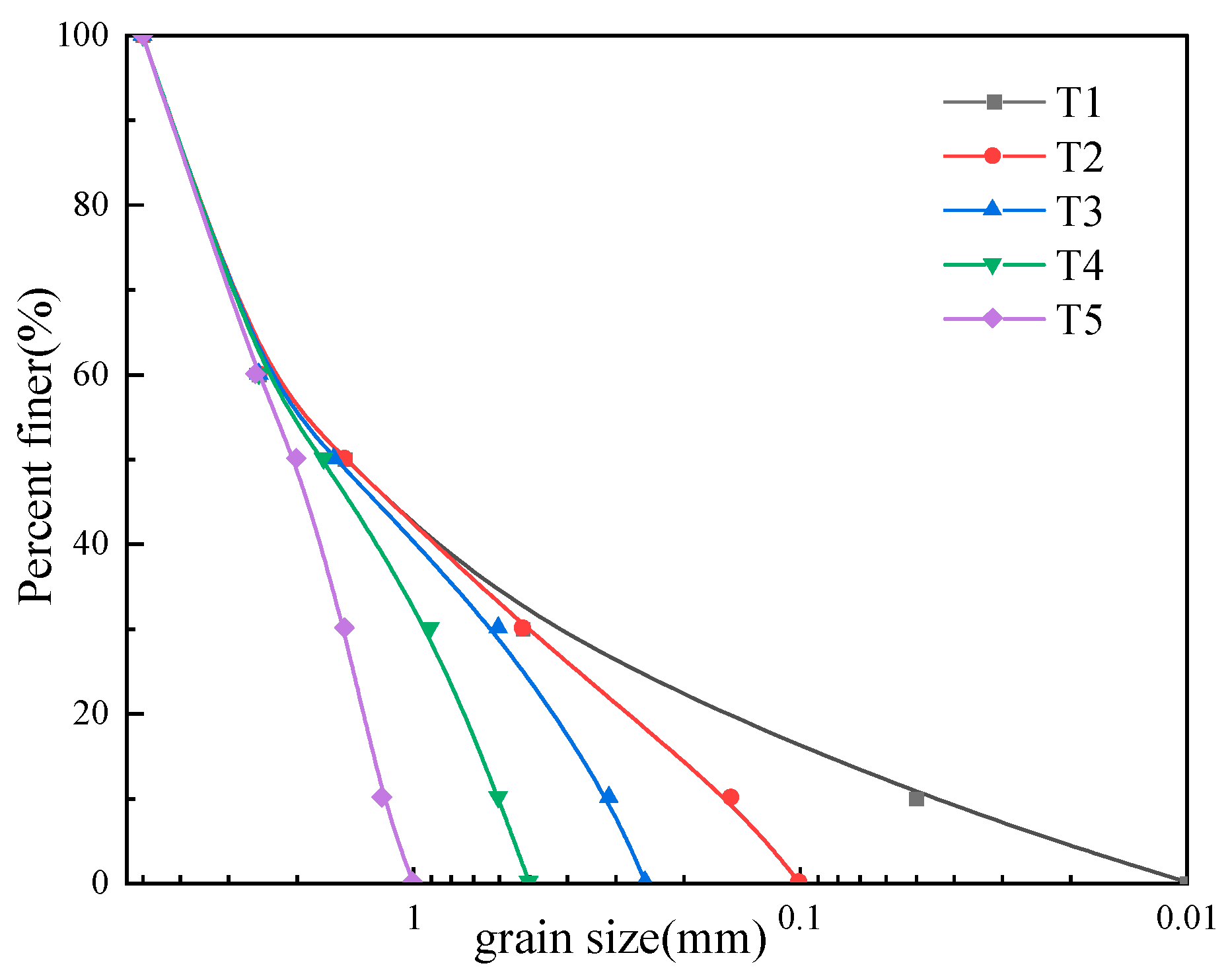
2.2. Sample Characteristics

The coral sand (CS) samples used in this experiment were collected from the reefs mentioned above. In contrast, the quartz sand (QS) samples used as the control group were obtained from a section of the upper reaches of the Yangtze River in China. The sand samples were dried and then subjected to vibrating sieve testing in accordance with the “Code for investigation of geotechnical engineering” (GB50021-2019) [34]. After sieving, six groups of coral and quartz sand samples with different particle sizes were obtained. Their distributions are shown in Figure 2. Figure 3 shows scanning electron microscope (SEM) images of the samples for each particle size group with the following magnification levels: 2000× for samples with particle sizes <0.1 mm, 800× for samples with particle sizes of 0.1–0.25 mm, 100× for samples with particle sizes of 0.25–2 mm, and 30× for samples with particle sizes of 2–5 mm. Based on the SEM images, we observed and analyzed the overall shape and surface characteristics of the CS and QS particles. The results indicate the following:

When the particle size is less than 0.25 mm, CS particles have a more regular overall shape and smoother surface than QS particles. When the particle size is between 0.25 and 1 mm, the overall shape of the CS particles is more regular than that of the QS particles, but their surfaces are rougher. When the particle size ranges from 1 to 5 mm, the CS particles are more irregular in shape and have rougher surfaces than the QS particles. Sand particles serve as the constituent units of the porous medium framework, and their shape and surface characteristics directly influence pore size, morphology, and connectivity. This determines the medium’s overall permeability. However, qualitative observations based on SEM images are insufficient to quantify the morphological differences between CS and QS particles. Therefore, building on the aforementioned qualitative findings, this study conducted three-dimensional particle morphology scanning experiments on samples of CS and QS to characterize their microscopic morphological features more precisely.

2.3. Sample Preparation

The sand samples used in this study are divided into two categories: six groups of single-grain sand and five groups of graded sand. Figure 2 shows the grain size distribution of the six groups of single-grain-size sand samples. The grading curves for the five graded sand sample groups (Figure 4) were designed based on the grading curves for the original sand samples from the reefs in the study area. This was conducted to systematically investigate the influence of the fine-grain content on the samples’ dispersion characteristics. For the comparative analysis, each CS test was accompanied by a QS control test with the same particle size or gradation.

Sample preparation used the layered compaction method, strictly controlling the dry density of the samples (${\rho }_d$ = 1.3 g/cm³). The specific steps are as follows:

(1)

Pre-wetting: Before filling the sample, add 5% of the dry sand’s mass to freshwater and mix it with the dry sand. Mix thoroughly to achieve a slightly moist state. This reduces the particle segregation during filling.

(2)

Layered filling: Divide the required sand volume into five equal layers based on the height of the sample cylinder. Pour the first layer of moist sand evenly into the sample cylinder.

(3)

Compaction within layers: Gently tap the side walls of the sample cylinder with a rubber hammer until the top surface of the sand layer reaches the predefined layer height mark. The tapping force must be consistent to avoid disturbing the already compacted layers.

(4)

Interlayer treatment: Before adding the next layer of sand, use a scraper to roughen the surface of the compacted sand layer, enhancing the interlayer bonding.

(5)

Repeat filling: Repeat steps 2 to 4 to sequentially fill and compact the remaining sand layers until the target sample height is reached.

The entire sample filling process must ensure that the final dry density of the sample is controlled within the range of 1.3 ± 0.02 g/cm³ (verified by calculating the mass and volume of the sample).

3. The Experimental Methodology

3.1. The One-Dimensional Dispersion Test

The coefficient of dispersion (COD) is an indicator that characterizes the dispersion of soluble substances through porous media, and it is related to the medium’s structure, the uniformity of the permeation pathway, the average permeation rate, and the physical and chemical properties of the fluid. Hydrodynamic dispersion comprises two mechanisms: mechanical dispersion and molecular diffusion [35]. Mechanical dispersion is a mechanical mixing process for fluid in porous media through a pore space, and it is related to the flow of water in porous media (mainly in terms of the flow rate distribution and average flow rate) and the characteristics of the pore structure. Molecular diffusion is the transport of matter in space caused by the thermal motion of molecules and atoms, driven by concentration differences or other forces, and it is related to the magnitude of the driving force and the temperature. The diffusion of molecules in soil media is hindered by pores [21].

This study involved a one-dimensional dispersion test of coral and quartz sands of various grain sizes. The specimens consisted of two types: six grain groups of coral sand (CS) and five groups of graded CS. Each CS test was accompanied by a QS control test. The specific test program is presented in

Table 1. One-dimensional dispersion test program.

Sand Type	Gradation	Dry Density (g/cm3)	C(NaCl) g/L
1	0–0.1 mm	1.3	20
2	0.1–0.25 mm
3	0.25–0.5 mm
4	0.5–1 mm
5	1–2 mm
6	2–5 mm
7	T1 (d60 = 2.50, d30 = 0.52, d10 = 0.05)
8	T2 (d60 = 2.50, d30 = 0.52, d10 = 0.15)
9	T3 (d60 = 2.50, d30 = 0.60, d10 = 0.31)
10	T4 (d60 = 2.50, d30 = 0.90, d10 = 0.60)
11	T5 (d60 = 2.55, d30 = 1.5, d10 = 1.2)

. The tests were performed using a one-dimensional dispersion test setup designed and fabricated independently, which is shown schematically in Figure 5. This setup allowed for three parallel tests to be performed for each set of tests. Thus, the CODs presented in this study are the averages of three parallel tests. The test device consisted of four parts, namely a dispersion bucket, a freshwater tank, a tracer tank, and a data acquisition system. The dispersion bucket was made of Plexiglas. It had an inner diameter of 8 cm and a height of 50 cm, serving as the main component of the dispersion test. A 5 cm glass bead buffer layer was placed at the top and bottom of the sample. The glass beads had diameters of 1 cm, which did not hinder permeation but did cause the cross-section of the soil sample to be uniformly permeated by the liquid. The data acquisition system consisted of a CS655 three-parameter sensor [36] and a CSI CR1000 data acquisition instrument [37], which simultaneously measured and recorded volumetric water content, temperature, and conductivity data. A 20 g/L NaCL solution was used as the tracer. The method of continuously injecting the tracer and collecting the test data at fixed positions was adopted in the test.

To initiate the test, the sample in the dispersion bucket was saturated with freshwater. Afterward, the freshwater supply valve was closed, the tracer supply valve was opened, and data acquisition began simultaneously. The relative NaCL concentration was calculated according to C = (C_cj − C₀)/(C_max − C₀), where C_cj is the NaCL concentration at time j, C₀ is the NaCL concentration at the initial time, and C_max is the maximum concentration in the test (the final steady-state concentration). The COD was calculated using the following formula [21]:

$$D_L={\displaystyle \frac{1}{8}}{\left[{\displaystyle \frac{x-u{t}_{0.1587}}{\sqrt{t_{0.1587}}}}-{\displaystyle \frac{x-u{t}_{0.8413}}{\sqrt{t_{0.8413}}}}\right]}^2$$

(1)

where D_L is the longitudinal COD, in cm²/s; x is the distance from the multi-parameter sensor to the tracer injection port, in cm; u is the average flow rate of the pore solution in the soil column, in cm/s; t_0.1587 is the time corresponding to (C_cj − C₀)/(C_max − C₀) = 0.1587, in s; and t_0.8413 is the time corresponding to (C_cj − C₀)/(C_max − C₀) = 0.841, in s.

3.2. The Molecular Diffusion Test

Molecular diffusion is a phenomenon in which solute molecules undergo random thermal motion due to a concentration difference or other driving forces, and it is influenced by the magnitude of the driving force and temperature. In porous media, the dispersion was molecular diffusion when the average pore flow rate was 0. The choice of tracer and sensor was the same as that in the one-dimensional dispersion test. Figure 6 shows the independently designed and manufactured molecular diffusion device. The device consisted of two parts (the left side and right side), each measuring 10 cm × 10 cm × 10 cm. The sample for the left part was saturated with NaCl solution, and the sample for the right part was saturated with freshwater. A control partition was placed in the middle. After the partition was lifted, molecular diffusion occurred between the pore solutions on the left and right sides under the concentration gradient. The timing and the data reading started at the same time as the partition was lifted, where E_N−t and E_W−t were the measured conductivities on the left and right sides at time t, and E_M−t = (E_N−t + E_W−t)/2 was the median value of the conductivity measured at time t. The molecular diffusion tests consisted of six grain groups of specimens made of either CS or QS. All specimens had a dry density of 1.3 g/cm³. The specific test protocols are shown in

Table 2. Experimental scheme of molecular diffusion.

Sand Type	Gradation	Dry Density (g/cm3)	C(NaCl) g/L
1	0–0.1 mm	1.3	20
2	0.1–0.25 mm
3	0.25–0.5 mm
4	0.5–1 mm
5	1–2 mm

.

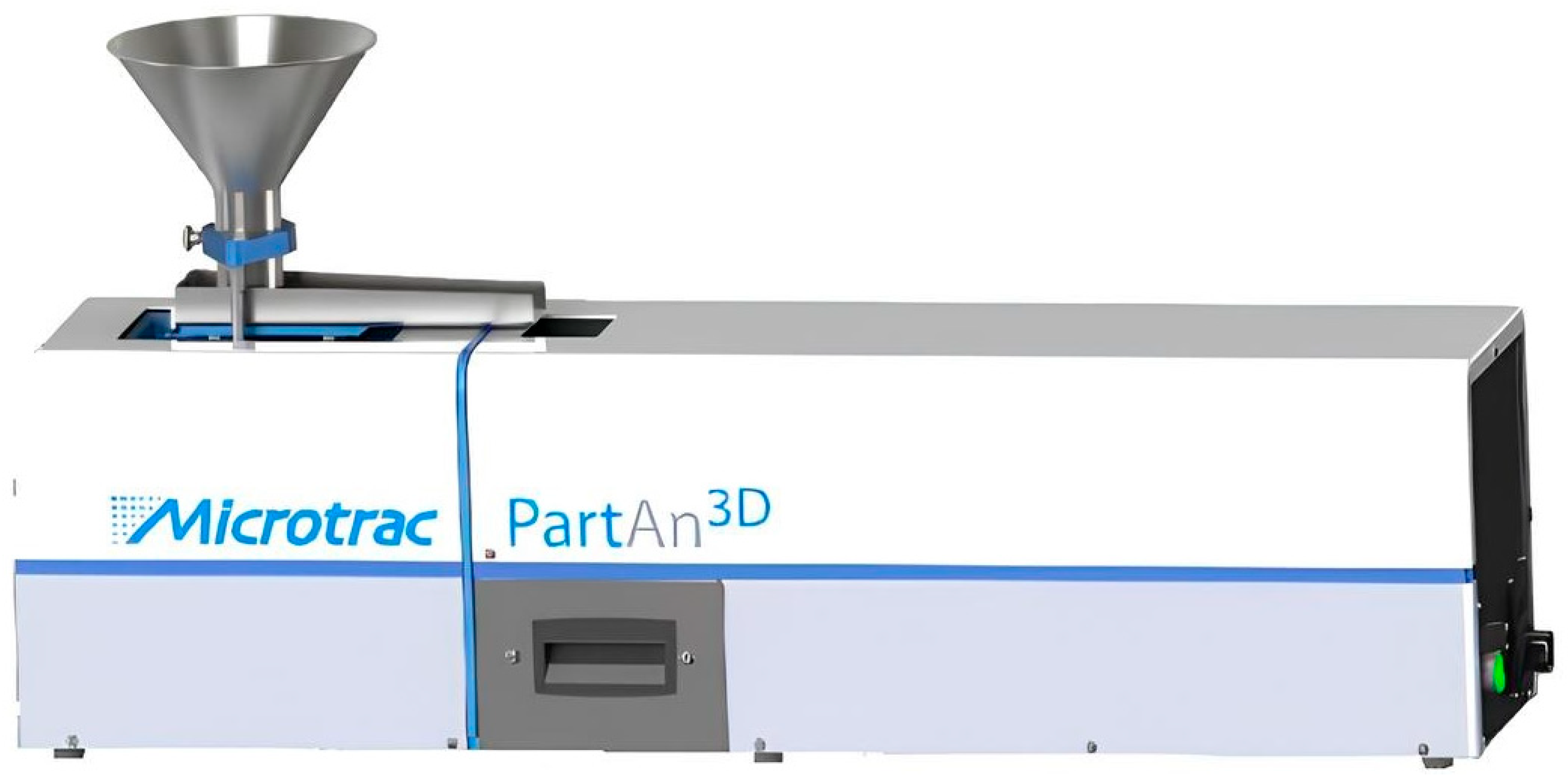
3.3. The Particle Morphology Analysis Test

The samples’ particle morphology was quantified using the PartAn^3D dynamic particle image analysis system produced by Microtrac, Inc., in Largo, FL, USA (Figure 7). This system is equipped with a high-resolution camera capable of capturing images at a maximum rate of 100 frames per second (fps) and has a resolution of 2056 × 2048 pixels. The system can measure particle sizes ranging from 22 to 35,000 μm.

During testing, sand particles are fed into a free-fall channel via an internal vibrating feeder. As the particles fall freely, the system captures two-dimensional images of the particles from multiple angles. The accompanying PartDP (v10.06) image processing software uses these images to create three-dimensional models of the particles. It automatically calculates over 30 particle sizes and morphological parameters (e.g., the Feret diameter, convexity, and aspect ratio).

To obtain statistically significant particle morphology characteristics, this study analyzed the morphology of all sand sample types before testing. Each analysis used a representative sample mass of 2000 g to ensure that the number of analyzed particles exceeded 30,000. For each morphological parameter, the median value of its cumulative distribution was used as the representative value for subsequent analyses.

4. Characterization of Granular Properties

4.1. The Particle Contact Surface Properties

The zeta potential characterizes the surface charge properties of particles and determines the strength of the electrostatic repulsion between them. This parameter affects the stability of particle systems and consequently the dispersion characteristics of sand samples. Zeta potential results are classified as positive or negative, with the sign indicating the type of charge on the particles and the absolute value representing the magnitude of the force. The smaller the absolute value is, the more likely the particles are to aggregate. Figure 8 shows the results of the zeta potential test. The curve in the figure is the zeta potential distribution curve for the test material, with the peak of the curve being the zeta potential (mV) of the test material. As shown in Figure 8, the zeta potential of the CS was −11.4 mV, indicating that the particles were negatively charged, while the zeta potential of the QS was 3.34 mV, indicating that the particles were positively charged. The absolute value of the zeta potential of QS is smaller than that of CS, which indicates that the electrostatic repulsive force between QS particles is weaker. Therefore, QS particles are more likely to overcome the weaker repulsive force and aggregate. Aggregation reduces the adequate pore size and increases pore tortuosity, decreasing the permeability of the porous medium. The zeta potential results from this study clearly show that due to their stronger electrostatic repulsive forces, CS particles are more likely to remain dispersed. This microscopic mechanism explains their superior dispersion properties compared to those of QS in terms of their charge properties.

4.2. Particle Contact Angle Characterization

The contact angle (θ) [38] is the angle formed by the tangent lines of the liquid and particle surfaces at the air–particle–liquid three-phase contact point, as shown in Figure 9. It is a key parameter for characterizing the wettability of solid particle surfaces: a smaller contact angle (θ < 90°) indicates stronger hydrophilicity, where the liquid spreads across the solid surface, while a larger contact angle (θ ≥ 90°) indicates stronger hydrophobicity, where the liquid forms droplets. The magnitude of the contact angle directly influences the flow behavior and microscopic driving forces of the liquid within pore channels, thereby significantly affecting the macroscopic dispersion characteristics of porous media. The test results show that the contact angle of CS (27.4–27.5°) is larger than that of QS (18.7–19.9°). Therefore, CS particles are less hydrophilic than QS particles. The hydrophilicity of the particles’ surface affects the resistance to the flow of liquid through the surface, resulting in different permeabilities in porous media.

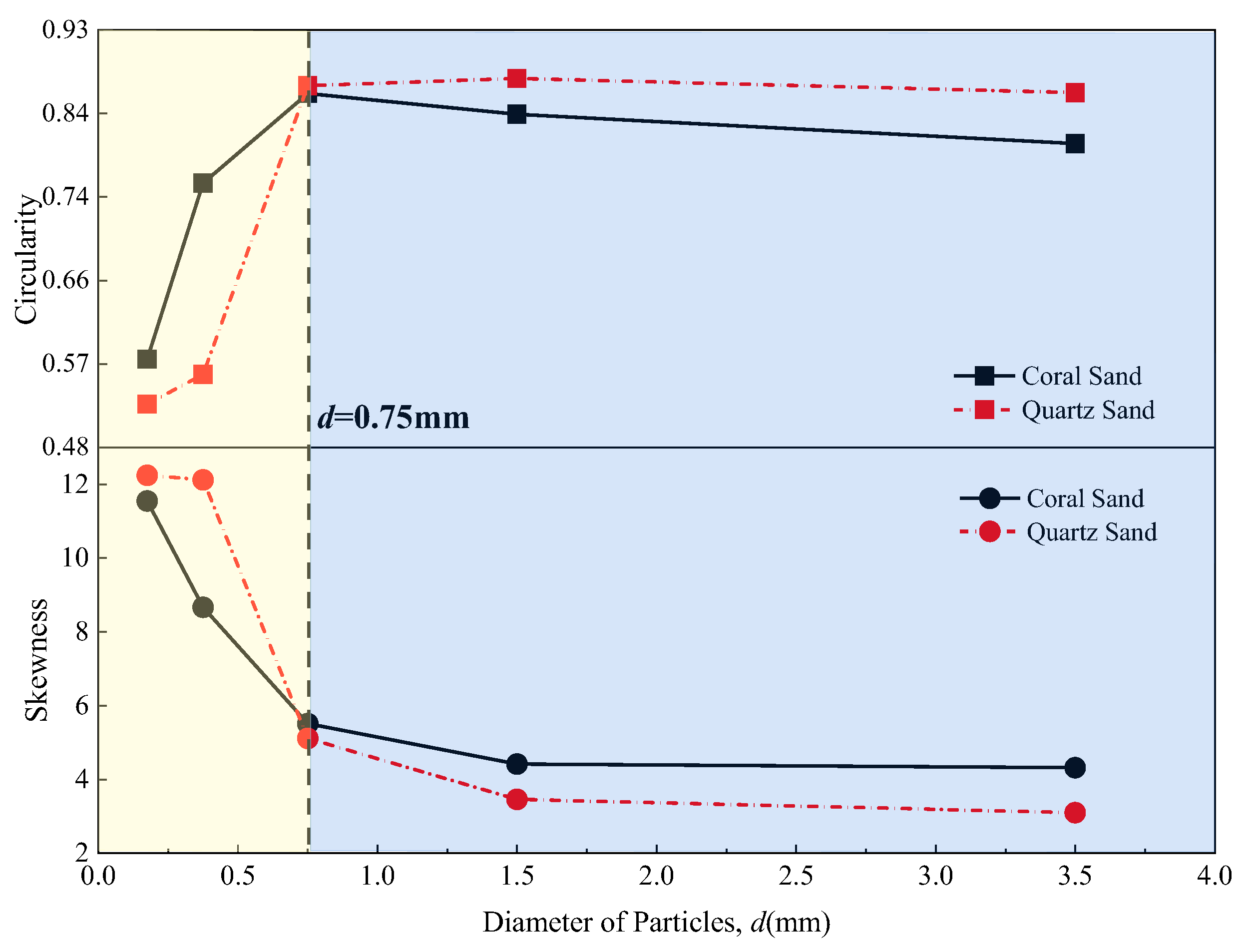
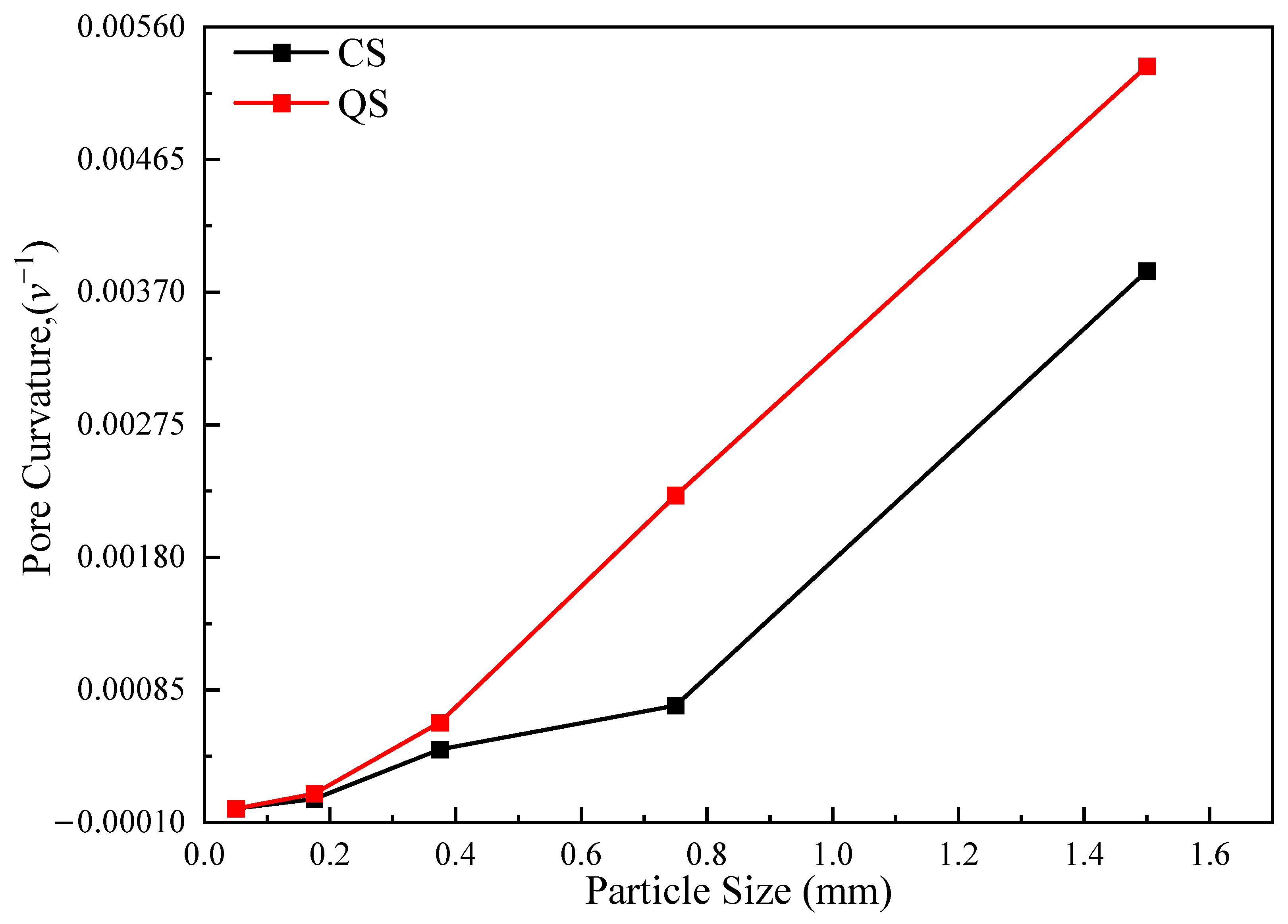
4.3. Particle Morphology Characteristics

The parameters obtained through the PartAn^3D test include both direct and indirect parameters. Direct parameters are obtained directly through image processing.

Table 3. Directly observed morphology parameters.

Parameter	Symbol (Unit)	Description	Illustration
Area	A (mm2)	Average particle image area
Perimeter	P (mm)	Average particle image perimeter
Feret length (FLength)	FL (mm)	The maximum length of the parallel tangent to the outer boundary of the particle
Feret width (FWidth)	FW (mm)	The maximum width of the parallel tangent to the outer boundary of the particle
Feret thickness (FThickness)	FT (mm)	The minimum width of the parallel tangent to the outer boundary of the particle
Convex hull area (CHull Area)	CA (mm2)	The area of the smallest convex boundary around the particle
Convex hull perimeter (CHull Perimeter)	CP (mm)	The perimeter of the smallest convex boundary around the particle

shows some commonly used direct parameters.

The indirect parameters were those calculated from the direct parameters. According to the test results, four indirect parameters (circularity, skewness, concavity, and convexity) were selected in this study to analyze the morphological differences between the CS and the QS. The circularity and the skewness characterized the difference between the overall shape of the particle and the standard sphere, and they were collectively referred to as the roundness (Φ). The larger the Φ value was, the more irregular the shape of a particle was. The concavity and the convexity characterized the undulation of the surface of a particle, and they were collectively referred to as the roughness (Ψ). The larger the Ψ value was, the rougher the particle surface was. The four indirect parameters were calculated using the following formulas:

$$\left\{\begin{array}{c}Cir={\displaystyle \frac{4\mathsf{\pi }\mathrm{A}}{P^2}}\\ Ske={\displaystyle \frac{{FL}^2}{\mathrm{F}\mathrm{W}\times \mathrm{F}\mathrm{T}}}\\ C_{\mathrm{c}}={\displaystyle \frac{\mathrm{C}\mathrm{A}-\mathrm{A}}{\mathrm{C}\mathrm{A}}}\\ C_{\mathrm{v}}={\displaystyle \frac{\mathrm{C}\mathrm{P}}{\mathrm{P}}}\end{array}\right.$$

(2)

where Cir is the circularity, which ranges from 0 to 1, with 1 representing a standard sphere; Ske is the skewness, which is ≥1, with 1 representing a standard sphere; C_c is the concavity, which ranges from 0 to 1, with 0 indicating that the particle surface is absolutely smooth; and C_v is the convexity, which ranges from 0 to 1, with 1 indicating that the particle surface is absolutely smooth. The meanings of the other parameters are shown in Table 3.

The scanned objects were CS and QS particles of five sizes: 0.1 mm to 0.25 mm, 0.25 mm to 0.5 mm, 0.5 mm to 1 mm, 1 mm to 2 mm, and 2 mm to 5 mm. In total, more than 30,000 particles were scanned at each particle size level. The direct parameters for each particle were substituted into Formula (2) to calculate the indirect parameters, and the arithmetic average of each indirect parameter was calculated to represent the comprehensive morphological parameters for a particle size. Figure 10 and Figure 11 show the morphology scanning results for the CS and QS particles.

As shown in Figure 10, when the particle size was less than 0.75 mm, the overall shape of the CS was more regular than that of the QS. When the particle size was greater than 0.75 mm, the overall shape of the CS was more irregular than that of the QS. As shown in Figure 11, when the particle size was less than 0.25 mm, the surface of the CS particles was smoother than that of the QS. When the particle size was greater than 0.25 mm, the surface of the CS particles was rougher than that of the QS particles. According to the observations in Figure 10 and Figure 11, the overall morphological patterns for the CS and QS particles were as follows. When the particle size was less than 0.25 mm, the CS had more regular particle shapes and smoother particle surfaces than those of the QS. When the particle size was in the range of 0.25 mm to 0.75 mm, the CS had more regular particle shapes but rougher particle surfaces than those of the QS. When the particle size was larger than 0.75 mm, the CS had more irregular particle shapes and rougher particle surfaces than those of the QS. In summary, within different particle size ranges, CS and QS exhibit different permeability advantages due to their differing shapes.

5. Analysis of the Dispersion Characteristics

5.1. Analysis of the Coefficient of Dispersion (COD)

Figure 12a shows the variation curve for the CODs of the coral sand (CS) and the quartz sand (QS) with particle size. As can be seen, the overall trend in the two curves was that the CODs of the CS and QS initially increased and then stabilized with an increase in particle size. This was because the solute dispersion in the porous media was mainly constrained by pores in the rising phase of the curve. As the particle size increased, the pores increased, and the dispersion was enhanced. When the particle size increased to a certain extent, the constraint of solute dispersion by the pores weakened, and the COD tended to stabilize. As shown in Figure 12a, the COD for CS is greater than that for QS when the particle size is less than 0.25 mm. Conversely, when the particle size is greater than 0.25 mm, the COD for CS is smaller than that for QS. These results are consistent with the PartAn^3D particle morphology scanning results in Section 4.3. CS has more regular particle shapes and smoother surfaces than those in QS when the particle size is less than 0.25 mm. Furthermore, CS has hydrophobic surfaces and is less likely to aggregate. As a result, its COD is higher when the particle size is less than 0.25 mm. When the particle size exceeds 0.25 mm, CS retains a porous skeleton, resulting in significantly increased surface roughness. While it still has a hydrophobic advantage, the rough surface significantly inhibits fluid migration, resulting in a lower COD than that for QS.

Figure 12b illustrates the disparity in the CODs between coral and quartz sands. It was found that the COD for the CS was vastly different from that for the QS in the range of intermediate particle sizes. As the particle size increased, the difference between the CODs of the two gradually decreased. This was because the difference in pore shape caused by the difference in particle shape was the dominant factor affecting the COD in the range of intermediate particle sizes. As the particle size increased gradually, the particle shape remained the dominant factor, but its influence on dispersivity decreased, and the difference between the CODs of the two decreased accordingly.

In summary, when the particle diameter was less than 0.25 mm, the roundness, the roughness, and the particle surface charge and hydrophilicity were all the main factors affecting the dispersion characteristics of the porous media. When the particle size was larger than 0.25 mm, the difference in roughness was the main factor affecting the dispersion characteristics. The roundness and the particle surface chargeability and hydrophilicity were the secondary factors affecting the dispersivity of the CS.

Figure 13 shows the COD curves for coral sand (CS) and quartz sand (QS) with different gradations. As shown in the figure, the COD for QS was larger than that for CS. However, as the fine-grain content gradually increased, the relative magnitudes of the CODs of the two tended to be opposite. In addition, as the gradation became coarser, the difference between the CODs of the two gradually decreased, following the same mechanism as stated above.

5.2. Molecular Diffusion

Figure 14 shows the molecular diffusion curves for coral sand (CS) and quartz sand (QS). Overall, after the final steady state was reached, the pore solution concentrations in the soil on the left and right sides had not completely reached equilibrium. Additionally, as the particle size decreased, the difference in concentrations between the left and right sides in the final steady state increased. This was because the solution needed to overcome the “resistance” of the porous media when the solution was dispersed in the porous media under the “driving force” of the concentration gradient. This hindering effect was enhanced as the particle size of the porous media decreased. When the driving force was less than the resistance, the dispersion was not able to change the concentration any further. This also explains the existence of a brackish water transition zone between freshwater lenses and the seawater beneath reefs. In practical applications, particle size has a significant impact on molecular diffusion. Smaller particles correspond to denser, more tortuous pore structures. These structures result in longer diffusion paths and greater resistance for solute molecules. This manifests as reduced pore tortuosity and slower diffusion rates. This phenomenon has been verified under laboratory conditions and holds significant implications for the formation of freshwater lenses in coral reefs. For instance, fine-grained sediments typically have lower permeability and slower solute migration rates, influencing the diffusion rate of brackish water and the size of the freshwater lenses in coral reefs. Therefore, understanding the relationship between particle size and molecular diffusion can help optimize the management of groundwater resources and protect the ecology of coral reefs.

To quantitatively characterize the hindering effect of the porous media on molecular diffusion, the concept of pore curvature (θ) is introduced here. Pore curvature is the ratio of the length of a medium to the length of the actual motion path of fluid particles [39], which is calculated as follows:

$$\theta ={\displaystyle \frac{S}{V\ast t}}$$

(3)

where S is the length of the porous medium (cm), V is the velocity of the fluid particles (cm/s) (here, the velocity is a scalar and its direction is not considered), and t is the time of the fluid particles’ motion(s). The above formula shows that the larger the actual distance traveled by the solute molecules, the smaller the pore curvature (θ).

The time (t) for each group of molecular diffusion tests to reach the final steady state was obtained from the data in Figure 15. The time was taken as infinity when the particle size was less than 0.1 mm. The distance from the sensor to the center partition is 4.9 cm, which is also the length of the porous medium. The curve for the pore curvature–granule size relationship can be obtained through substitution into Equation (3), as shown in Figure 15. The distribution range for the pore curvature in this study is 0–0.0055, consistent with existing studies that show that pore curvature takes a value in the range of 0–0.5 [40]. As defined above, the smaller the pore curvature, the greater the “resistance” of the porous medium to solute dispersion. In Figure 15, the QS curve is above the CS curve, indicating that the pore curvature of CS is smaller than that of QS for the same grain size. Thus, the “resistance” of CS to solute dispersion is greater than that of QS. This is consistent with the law of the COD described in Section 4.1. At the same time, the results of the analysis in this study show that pore curvature, particle size, and shape are closely related. Drawing on results from existing research, the pore curvature value for clay is 0.1, and that of sand is 0.7 [41]. However, these values should be adjusted based on the type of sand sample and particle size.

5.3. COD Conversion

According to the research results described in Section 4.2, the primary and secondary factors in the piecewise patterns of the dispersion characteristics of CS and QS are shown in

Table 4. The factors controlling the difference in the hydrological parameters of CS and QS.

Parameter	Particle Size Range	Primary Factor	Secondary Factor
COD	<0.25 mm	Roundness Φ, roughness Ψ, particle surface charge, hydrophilicity	-
	>0.25 mm	Roughness Ψ	Roundness Φ, particle surface charge, hydrophilicity

.

The morphological data on the main and secondary factors corresponding to the particle size ranges in Table 4 were extracted in order to calculate the parameter conversion factor using the following formula:

$$\left\{\begin{array}{c}{P}_i={\displaystyle \frac{\left(M_{c,i}-M_{Q,i}\right)}{M_{Q,i}}}\\ \overline{P}={\displaystyle \frac{{\sum }_i{P}_i}{n}}\end{array}\right.$$

(4)

where P_i is the conversion factor for CS and QS in the particle size range i provided by the parameter M; Q represents QS; C represents CS; i is the particle size; n is the number of particle sizes involved in the calculation of the conversion factor; M_c,i is the microscopic parameter of the CS for particle size i (e.g., roundness, roughness, particle surface charge, hydrophilicity sphericality); M_Q,i is the microscopic parameter of the QS for particle size i (e.g., roundness, roughness, particle surface charge, hydrophilicity sphericality); and $\overline{P}$ is the conversion factor for the CS and QS within n particle size ranges provided by the parameter M. 

Table 5. The conversion factors for the COD of the CS and QS.

Particle Size Range	Major Factor	Conversion Factors	Minor Factor	Conversion Factor
<0.25 mm	Roundness	0.2020	-	-
	Roughness	0.2890
	Zeta potential	2.4132
	Contact angle	0.4223
≥0.25 mm	Roughness	0.4159	Roundness	0.1444
			Zeta potential	2.4132
			Contact angle	0.4223

Note: All of the data in the table was calculated using Formula (4).

shows the conversion factors for the CODs of the CS and QS.

The piecewise conversion functions for the CODs of the CS and QS, taking into account the conversion factors in Table 5, are presented below.

$$D_C=\left\{\begin{array}{c}\theta \times {\mathrm{l}\mathrm{n}(D}_Q)+\alpha ,L<0.25\mathrm{mm}\\ \beta \times D_Q+\mu ,L\ge 0.25\mathrm{mm}\end{array}\right.$$

(5)

where D_c is the COD of the CS, in cm/s; D_Q is the COD of the QS, in cm/s; L is the particle size, in mm; and θ, β, μ, and α are the conversion coefficients calculated using the conversion factors in Table 5, where $\theta =B^Z\times \mathrm{l}\mathrm{n}\left(Z\right)$, $\mathsf{\alpha }={\displaystyle \frac{A+C}{2}}$, $\beta =A+{\displaystyle \frac{A+Z+C}{3}}$, $\mu =B-{\displaystyle \frac{A+C+Z}{3}}$. A is the roundness conversion factor, B is the roughness conversion factor, C is the contact angle conversion factor, and Z is the zeta potential conversion factor.

By substituting the values of A, B, C, and Z into Formula (4), the CS and QS COD segmentation conversion function was obtained as in Formula (5):

$$D_C=\left\{\begin{array}{c}0.4406\times {\mathrm{l}\mathrm{n}(D}_Q)+0.3121,L<0.25\mathrm{mm}\\ 1.1377\times D_Q-0.5774,L\ge 0.25\mathrm{mm}\end{array}\right.$$

(6)

The conversion curve is plotted in Figure 16. Figure 16a shows the conversion curves for the CODs of the CS and the QS with particle sizes of less than 0.25 mm, and Figure 16b shows the conversion curves for the CODs of the CS and the QS with particle sizes larger than 0.25 mm. In coastal engineering projects [42], freshwater resource development on islands and reefs [43,44], and coral reef reclamation projects [45], the diffusion coefficient for CS can quickly be determined using the relationship between the diffusion coefficients for CS and QS shown in Figure 16. Thus, the accuracy and reliability of numerical simulations and engineering design are enhanced. Additionally, the conversion factors discussed in this study reveal how the morphology of CS particles influences the diffusion coefficient. This facilitates a deeper understanding of the solute migration processes in porous media. These findings have significant implications for assessing the impact of underground structures on freshwater lenses in reefs [46], coral reef pollutant leakage [47,48], and freshwater resource management.

6. Modeling and Sensitivity Analysis

6.1. Basic Information on the Model

A two-dimensional section model was established in this study, and the numerical simulation contained eight CODs, as shown in

Table 6. GMS numerical simulation scheme.

Variable	Values
Dispersivity (m)	1.5, 3, 3.5, 4, 4.5, 5, 5.5, 6

, for the specific scheme. A schematic diagram of the conceptual model is shown in Figure 17. The simulated elevation of the model ranged from the coral island–reef surface (5 m) to the interior of the reef limestone layer (−40 m) [3,13]. The complete model simulated the dual stratigraphic structure of the coral island–reef, with the elevation of the CS layer ranging from 5 m to 20 m and the elevation of the reef limestone layer ranging from −20 m to 40 m. The yellow line in Figure 17 is the boundary of the dual structure. The horizontal simulation range of the model was 1000 m. The trapezoidal part in the middle simulated a coral island–reef, and the low-lying parts on both sides simulated submarine reef flat facies. The values of the model’s hydrologic parameters are shown in

Table 7. Values assigned to the hydrogeological parameters of the model.

Parameter	Value
Permeability coefficient (m/d)	100 for CS, 1500 for reef limestone
Specific yield	0.25
Dispersivity (m)	5
Porosity	0.3
Elastic storativity	0.00001

Note: The parameters in the table are basic model parameters. Only dispersion varies in the parameter sensitivity analysis.

.

The boundary conditions were as follows. The top surface of the island–reef was set as a variable recharge boundary. The rainfall and evaporation data referred to the meteorological observation data (on a monthly scale from January to December 2018) from an island–reef in Xisha, China, with an effective infiltration coefficient of 0.6. The effective recharge was equal to the rainfall–evaporation multiplied by the effective infiltration coefficient, as shown in Figure 17. The effective infiltration coefficient was determined based on data from the existing literature [49,50]. The red line in Figure 17 was defined as the constant-concentration and variable-head boundary. The concentration was set to the chloride ion concentration of 19 g/L in seawater. The head value was taken from water level observation data (on a monthly scale from January to December 2018) for an island–reef in Xisha, China, as shown in Figure 18 [3]. The bottom boundary of the model, depicted as a brown line in Figure 17, was set at a depth of 40 m below the ground surface. Because the bottom boundary was hydraulically connected to the surrounding sea area and did not affect the formation and evolution of the lens, it was set to a zero-flow boundary.

The initial conditions were as follows. According to meteorological observation data (collected from January to December 2018) from an island–reef in Xisha, China, the annual average water level (1.2 m) was calculated as the initial water level value for the model. Below sea level, the initial concentration was set to 19 g/L of chloride ions. Above sea level, the initial concentration of the exposed part of the island–reef was set to a chloride ion concentration of 0 g/L.

The time was discretized as follows: 30 days were designated as a stress period, and there were 360 stress periods in total, resulting in a total simulation time of 10,800 days. The initial step size was set to 1 day, and the model was set to output calculation results every 30 days. In terms of meshing, the entire model was divided into 90 horizontal layers and 100 vertical layers, resulting in 9000 valid grid cells for the calculation.

In terms of the calculations, the SEAWAT module in GMS (version 10.4), which can solve the finite difference model for an unsteady flow with a variable density in porous media, was adopted. The primary method involved synchronizing the calculation steps for MODFLOW and MT3DMS to achieve a coupled solution for the water flow and solute transport equations. Therefore, the model employed two formulas to control the calculation.

(1)

The variable-density water flow formula was based on mass conservation and Darcy’s law:

$$K\left({\displaystyle \frac{{\partial }^{2}H}{\partial x^2}}+{\displaystyle \frac{{\partial }^{2}H}{\partial y^2}}+{\displaystyle \frac{{\partial }^{2}H}{\partial z^2}}\right)+K\eta {\displaystyle \frac{\partial c}{\partial z}}=S_s{\displaystyle \frac{\partial H}{\partial t}}+n\eta {\displaystyle \frac{\partial c}{\partial t}}-{\displaystyle \frac{\rho }{{\rho }_0}}{q}_s$$

(7)

where K is the permeability coefficient, in m/d; η is the density coupling coefficient, in kg/m³; H is the head, in m; S_s is the storativity; t is the time, in d; ρ is the density of the mixed fluid, in kg/m³; q_s is the source or sink intensity per unit volume of the porous medium, in d⁻¹; x, y, z represents the coordinates; and c is the concentration of the mixed fluid, in kg/m³;

(2)

The solute transport formula is as follows:

$${\displaystyle \frac{\partial c}{\partial t}}+u_i\left({\displaystyle \frac{\partial c}{\partial x_i}}\right)={\displaystyle \frac{\partial }{\partial x_i}}\left(D_{ii}{\displaystyle \frac{\partial c}{\partial x_i}}\right)+{\displaystyle \frac{c^{*}-c}{n}}{q}_s$$

(8)

where x, y, z represents the coordinates; t is the time, in d; n is the porosity of the porous medium; c is the concentration of the mixed fluid, in kg/m³; q_s is the source or sink intensity per unit volume of the porous medium, in d⁻¹; u_i is the permeation rate, in m/d; D_ii is the COD, in m²/d; and $c^{*}$ is the concentration of fluid produced by the source or the sink, in kg/m³.

6.2. Parameter Sensitivity Analysis Method

A sensitivity analysis refers to a qualitative or quantitative analysis of the response of simulation results caused by parameter variations. The analysis methods usually include local sensitivity analyses and global sensitivity analyses [51,52]. The regional analysis method involves varying the value of only one parameter in a model and using the degree of the response of the model results caused by the variation to represent the sensitivity of that parameter. For this reason, local sensitivity analysis is also known as the single-variation method [53]. The regional sensitivity analysis method was used in this study.

According to the study of a freshwater lens in an island–reef by Zhou et al. [54], a chloride ion concentration of 0.6 g/L was chosen as the maximum concentration in freshwater. Therefore, the freshwater body in this study refers to a groundwater body with a chloride ion concentration of 0.6 g/L or less. The freshwater lens refers to the groundwater body diluted by rainfall. The values of four parameters, namely the freshwater appearance time (d), the lens stabilization time (d), the steady-state freshwater reserve (m³), and the thickness of the steady-state freshwater body (m), were selected from the freshwater lens response results for the qualitative sensitivity analysis of the COD. Due to the significant differences in the order of magnitude among these four lens body response indicators mentioned above, a direct comparison is not feasible. Therefore, they are normalized. This eliminates dimensional differences and enables a direct comparison of cross-dimensional metrics, such as the freshwater emergence time (d), the lens stability time (d), the steady-state freshwater storage volume (m³), and the steady-state freshwater lens thickness (m). This avoids misinterpreting the parameter sensitivity rankings due to absolute changes in values. The dimensionless normalization formula is given by Formula (9).

$${\mathrm{S}}_{DG}={\displaystyle \frac{[{(G}_{i+1}-G_i)/G_i]}{\left[\frac{D_{i+1}-D_i}{D_i}\right]}}$$

(9)

In the formula, D is the COD; G is the lens response index (the freshwater appearance time (d), the lens stabilization time (d), the steady-state freshwater reserve (m³), or the steady-state freshwater body thickness (m)); i refers to the simulation of the COD from small to large within a reasonable range, so $N_{i+1}>N_i$; and S_DG is the influence of the COD on the index G. Because they were affected by the rainfall and the tide, the steady-state freshwater body thickness and the steady-state freshwater reserve were variable, their arithmetic average values were substituted into Formula (9) for calculation. The following formula was used to calculate the percentage of the maximum variation in the lens response index caused by the COD.

$$M_{DG}={\displaystyle \frac{\left[\max \left(G_D\right)-\min \left(G_D\right)\right]}{\min \left(G_D\right)}}$$

(10)

where the definition of D and G is the same as that in Formula (9); $\max \left(G_D\right) \mathrm{a}\mathrm{n}\mathrm{d} \mathrm{m}\mathrm{i}\mathrm{n}\left(G_D\right)$ are the maximum and minimum values, respectively, of the lens index G; and $M_{DG}$ is the percentage of the maximum variation in the lens index G.

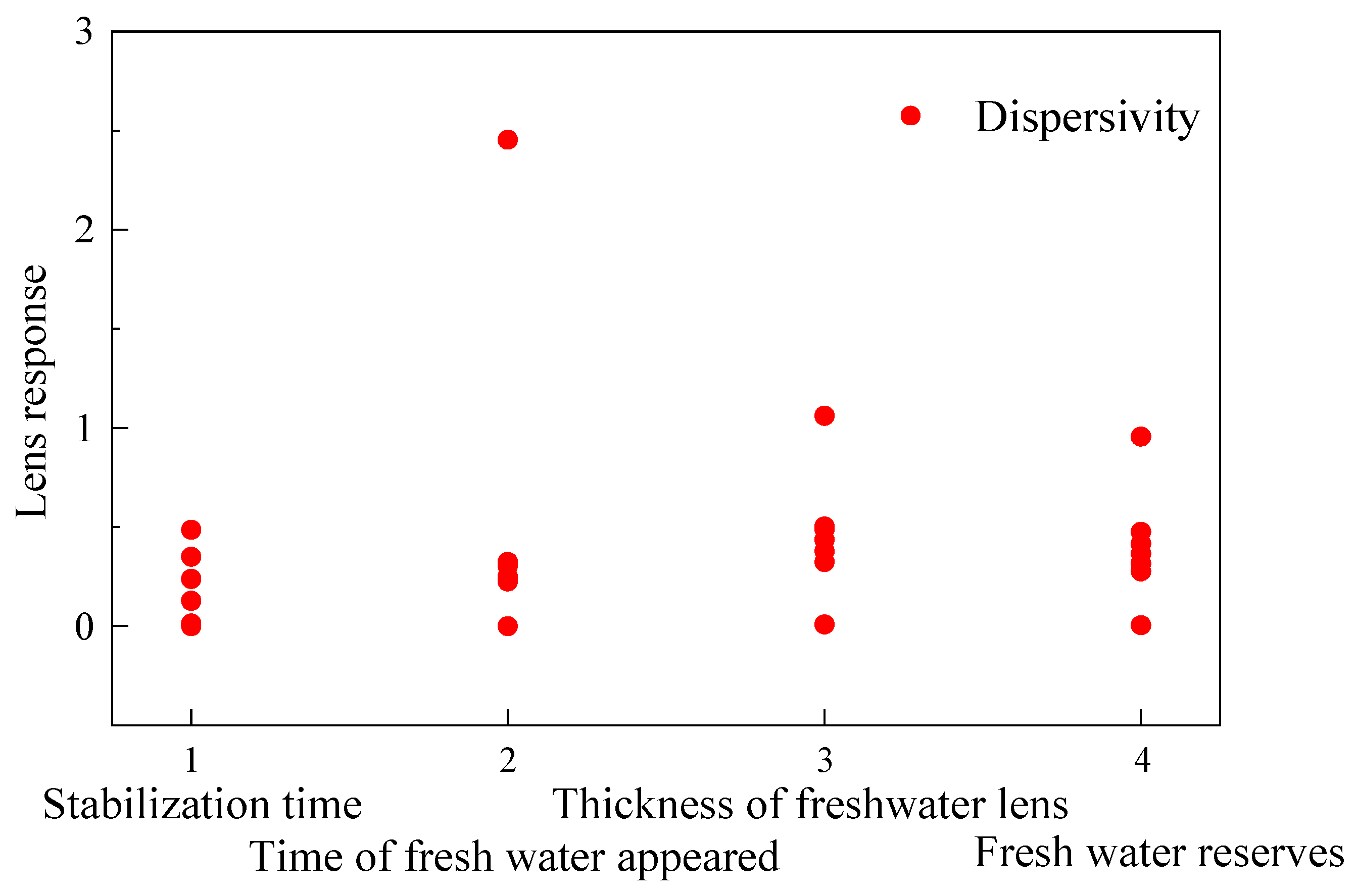
6.3. Sensitivity Analysis

6.3.1. The Freshwater Lens Response Patterns

The COD sensitivity analysis of the first layer (coral soil layer) in the conceptual model schematic diagram, as shown in Figure 17, was conducted using the local sensitivity analysis method. The values of four freshwater lens response indexes, i.e., freshwater appearance time, lens stabilization time, steady-state freshwater body thickness, and steady-state freshwater reserve, were selected in this study. Figure 19 shows the results of the basic model. For the basic model, the dispersivity was set to 5 m, the permeability coefficient was set to 100 m/d, and the specific yield was set to 0.25. The blue region in the figure is the final steady-state freshwater body. The observation well was positioned at the maximum thickness of the body, and seven observation points were established within the observation area. Because the factors of tidal variation and uneven rainfall were considered in the simulation process, it was defined that a steady state was reached when the variation in the concentration became cyclic and stable. When the concentration at each observation point was stable, it was determined that the freshwater lens had reached the final steady state.

Figure 20 illustrates the response pattern for each of the four freshwater lens indexes to dispersivity. As can be seen from the figure, as the dispersivity increased, the lens reaching a steady state was delayed, the appearance of freshwater was delayed, the lens thickness was reduced, and the freshwater reserve decreased. As long as the dispersivity was varied within a reasonable range, the phenomenon of the lens occurring intermittently and failing to form did not occur. This study quantitatively reveals how changes in the CODs impact the formation of freshwater lenses, a phenomenon closely associated with high-permeability CS aquifers. Sheng et al. [55] confirmed that high permeability accelerates the mixing of freshwater and saltwater in coral reefs, resulting in thinner lenses. Studies by Thissen [56] of coral reefs in the North Sea and by Bailey [57] of freshwater lenses in a CS atoll indicate that an increase in parameters such as the hydraulic conductivity is detrimental to the formation of freshwater lenses on islands. However, the underlying mechanisms are difficult to quantify. This study quantifies the role of CODs in freshwater lens formation on coral reefs, elucidates the diffusion mechanisms in the formation process, and provides a theoretical basis for developing groundwater resources on coral reefs.

6.3.2. Parameter Sensitivity Analysis Results

The data in Figure 20 were normalized using dimensionless normalization, as described by Formula (9). Figure 21 shows a scatter plot of the diffusion coefficient’s sensitivity after the lens body response index was dimensionlessly normalized. After dimensionless normalization using Formula (9), it can be seen that the four variables eliminate dimensional differences, making the sensitivity of parameters of different magnitudes more intuitive. This provides a basis for future studies on the diffusion characteristics of different coral reefs. The four points on the abscissa represent the (1) lens stabilization time, (2) freshwater appearance time, (3) steady-state freshwater body thickness, and (4) steady-state freshwater reserve. The ordinate represents the percentage response of the lens index with the unit percentage of variation in the hydrological parameters. The black dot denotes the lens response resulting from the variation in dispersivity. The larger the ordinate value was, the greater the influence of the variation in dispersivity on the lens was. It could be concluded from the figure that the sensitivity of the COD to the four indexes of the lens was ranked from high to low in the order of the freshwater appearance time > steady-state freshwater body thickness > steady-state freshwater reserve > lens stabilization time. This pattern aligns with Eeman’s conclusion [58] that dispersive properties are time-dependent in the formation of freshwater lenses.

According to Formula (10), the COD falls within a reasonable range.

Table 8. Maximum response of the lens during the variation of the hydrological parameters.

Lens Index	Minimum	Maximum	Range	Percentage (%)
Lens stabilization time (d)	3650	4350	700	19.17
Freshwater appearance time (d)	660	1050	390	59.09
Freshwater body thickness (d)	7.25	11.3	4.05	55.86
Freshwater reserve (m3)	197,304.48	28,9301.78	91,997.30	46.63

shows the maximum relative rates of change in the response indicators for each freshwater lens. As shown in Table 8, the sensitivity of each response indicator to the COD, ranked from highest to lowest, is as follows: freshwater appearance time > freshwater body thickness > freshwater reserve > lens stabilization time. These results indicate that the COD has a significant influence on the formation dynamics of freshwater lenses, regulating solute diffusion and transport processes. The results of this sensitivity analysis provide an essential basis for optimizing the parameters in subsequent hydrogeological models of islands.

7. Conclusions

This study systematically elucidated the formation mechanism behind the solute dispersion characteristics in coral sand (CS) media, as well as the control laws governing the evolution of freshwater lenses, through a combination of multi-scale experiments and numerical simulations. The main conclusions are as follows:

(1)

Based on comprehensive morphological characterization using PartAn^3D, the zeta potential, the particle contact angle, and other microscopic experiments, the main reasons for the difference in dispersion between coral sand and quartz sand (QS) were first revealed to be the difference in the roughness (Ψ), roundness (Φ), surface hydrophilicity (C), and particle charge (Z) of the particles. Additionally, it was found that the action of these four factors on the dispersive properties varies with particle size.

(2)

A transformation model for the coefficient of dispersion (COD) of coral sand and quartz sand was developed from a microscopic perspective, achieving a high degree of accuracy (R² > 0.99). This model overcomes the limitations of the traditional empirical formulas and can be directly integrated into numerical simulations of island reef engineering, thereby reducing the errors in freshwater lens reservoir assessments and enabling more precise predictions for resource development.

(3)

The results of the GMS numerical simulation quantitatively reveal the spatial and temporal control effects of the COD on the formation and evolution of freshwater lenses in the subsurface of coral reefs. The factors affecting the freshwater lens response, ranked by sensitivity, are as follows: freshwater appearance time, freshwater body thickness, freshwater reserve, and lens stabilization time. This sensitivity ranking provides a basis for prioritizing the management of freshwater development impacts on coral reefs.

This research achievement integrates the solute transport in coral sand at multiple scales, from microscopic characteristics to macroscopic responses. This deepens our theoretical understanding of solute transport in coral sand. These findings can inform the selection and grading of the fill materials for land reclamation and island construction projects. They can also provide scientific support for precisely predicting freshwater lenses in reefs and for the rational development and dynamic regulation of freshwater resources in reefs. Future work can focus on the impact of heterogeneity in the particle sizes of coral sand on freshwater lens bodies in islands and reefs. Additionally, future work could develop methods to optimize the dispersion characteristics of coral sand through surface modification. This would contribute to the secure management of water resources in island and reef engineering projects.

References

1. Sheng, C.; Jiao, J.J.; Xu, H.; Liu, Y.; Luo, X. Influence of Land Reclamation on Fresh Groundwater Lenses in Oceanic Islands: Laboratory and Numerical Validation. Water Resour. Res. 2021, 57, e2021WR030238. [Google Scholar] [CrossRef]
2. Tang, Y.; Yan, M.; Wang, X.; Lu, C.; Luo, J. Analytical Solutions for Fresh Groundwater Lenses in Small Strip Islands with Spatially Variable Recharge. Water Resour. Res. 2021, 57, e2020WR029497. [Google Scholar] [CrossRef]
3. Cui, X.; Qu, R.; Hu, M. Response of Freshwater Lenses to Precipitation and Tides. J. Mar. Sci. Eng. 2025, 13, 738. [Google Scholar] [CrossRef]
4. Tang, Y.; Lu, C.; Luo, J. Optimizing Groundwater Pumping in Small Island Groundwater Lenses: An Analytical Approach. J. Hydrol. 2024, 629, 130579. [Google Scholar] [CrossRef]
5. Ju, Y.; Hu, M.; Liu, Y.; Zhu, X.; Qin, K. Formation Process of Underground Freshwater Based on Zoning and Stratification of Coral Reef Island. Rock Soil Mech. 2022, 43, 1226–1236. [Google Scholar] [CrossRef]
6. Babu, R.; Park, N.; Nam, B. Regional and Well-Scale Indicators for Assessing the Sustainability of Small Island Fresh Groundwater Lenses under Future Climate Conditions. Environ. Earth Sci. 2020, 79, 47. [Google Scholar] [CrossRef]
7. Werner, A.D.; Sharp, H.K.; Galvis, S.C.; Post, V.E.A.; Sinclair, P. Hydrogeology and Management of Freshwater Lenses on Atoll Islands: Review of Current Knowledge and Research Needs. J. Hydrol. 2017, 551, 819–844. [Google Scholar] [CrossRef]
8. Wang, X.; Weng, Y.; Wei, H.; Meng, Q.; Hu, M. Particle Obstruction and Crushing of Dredged Calcareous Soil in the Nansha Islands, South China Sea. Eng. Geol. 2019, 261, 105274. [Google Scholar] [CrossRef]
9. Wang, X.; Ding, H.; Wen, D.; Wang, X. Vibroflotation Method to Improve Silt Interlayers of Dredged Coral Sand Ground–a Case Study. Bull. Eng. Geol. Environ. 2022, 81, 472. [Google Scholar] [CrossRef]
10. Qu, R.; Ma, C.; Liu, H.; Zhu, C.; Hu, T. Triaxial Test on Load-Bear Capacity of the Vibro-Compaction Coral Sand Foundation in the South China Sea. Appl. Ocean Res. 2024, 153, 104321. [Google Scholar] [CrossRef]
11. Chen, X.; Shen, J.; Wang, X.; Yao, T.; Xu, D. Effect of Saturation on Shear Behavior and Particle Breakage of Coral Sand. J. Mar. Sci. Eng. 2022, 10, 1280. [Google Scholar] [CrossRef]
12. Wang, Y.; Ren, Y.; Yang, Q. Experimental Study on the Hydraulic Conductivity of Calcareous Sand in South China Sea. Mar. Geores. Geotechnol. 2017, 35, 1037–1047. [Google Scholar] [CrossRef]
13. Zhu, C.; Liu, H.; Zhou, B. Micro-Structures and the Basic Engineering Properties of Beach Calcarenites in South China Sea. Ocean Eng. 2016, 114, 224–235. [Google Scholar] [CrossRef]
14. Cheng, Z.; Wang, J. An Investigation of the Breakage Behaviour of a Pre-Crushed Carbonate Sand under Shear Using X-Ray Micro-Tomography. Eng. Geol. 2021, 293, 106286. [Google Scholar] [CrossRef]
15. Cui, X.; Zhu, C.; Hu, M.; Wang, R.; Liu, H. Permeability of Porous Media in Coral Reefs. Bull. Eng. Geol. Environ. 2021, 80, 5111–5126. [Google Scholar] [CrossRef]
16. Gao, C.; Zheng, T.; Chang, Q.; Zhang, J.; Hao, Y.; Cao, M.; Zheng, X.; Luo, J. Fresh Groundwater Lens Evolution in Artificial Islands Accompanied with Silt Uplift. Phys. Fluids 2025, 37, 016611. [Google Scholar] [CrossRef]
17. Zhao, Y.; Zhang, Z.; Rong, R.; Dong, X.; Wang, J. A New Calculation Method for Hydrogeological Parameters from Unsteady-Flow Pumping Tests with a Circular Constant Water-Head Boundary of Finite Scale. Q. J. Eng. Geol. Hydrogeol. 2022, 55, qjegh2021-112. [Google Scholar] [CrossRef]
18. Lin, H.-T.; Tan, Y.-C.; Chen, C.-H.; Yu, H.-L.; Wu, S.-C.; Ke, K.-Y. Estimation of Effective Hydrogeological Parameters in Heterogeneous and Anisotropic Aquifers. J. Hydrol. 2010, 389, 57–68. [Google Scholar] [CrossRef]
19. Egbert, G.D. Tidal Data Inversion: Interpolation and Inference. Prog. Oceanogr. 1997, 40, 53–80. [Google Scholar] [CrossRef]
20. Sheng, C.; Han, D.; Xu, H.; Li, F.; Zhang, Y.; Shen, Y. Evaluating Dynamic Mechanisms and Formation Process of Freshwater Lenses on Reclaimed Atoll Islands in the South China Sea. J. Hydrol. 2020, 584, 124641. [Google Scholar] [CrossRef]
21. Cui, X.; Zhu, C.; Hu, M.; Wang, X.; Liu, H. The Hydrodynamic Dispersion Characteristics of Coral Sands. J. Mar. Sci. Eng. 2019, 7, 291. [Google Scholar] [CrossRef]
22. Parker, J.; Vangenuchten, M. Determining Transport Parameters from Laboratory and Field Tracer Experiments; Bulletin 84-3; Virginia Agricultural Experiment Station: Glade Spring, GA, USA, 1984; pp. 1–96. [Google Scholar]
23. Jensen, K.H.; Destouni, G.; Sassner, M. Advection-Dispersion Analysis of Solute Transport in Undisturbed Soil Monoliths. Ground Water 1996, 34, 1090–1097. [Google Scholar] [CrossRef]
24. Zhang, J.; Wang, M. Investigation of the relation between longitudinal dispersion and heterogeneity using the numerical simulation approach. Earth Sci. Front. 2010, 17, 152–158. [Google Scholar]
25. Sahimi, M. Fractal and Superdiffusive Transport and Hydrodynamic Dispersion in Heterogeneous Porous-Media. Transp. Porous Media 1993, 13, 3–40. [Google Scholar] [CrossRef]
26. Sahimi, M. Comment on Fractal and Superdiffusive Transport and Hydrodynamic Dispersion in Heterogeneous Porous-Media—Reply. Transp. Porous Media 1995, 21, 189–194. [Google Scholar] [CrossRef]
27. Zhang, H.; Jia, D. Calculation of hydrodynamic dispersion coefficients under one-dimensional unsaturated conditions. Irrig. Drain. 1987, 1987, 8–15. (In Chinese). Available online: https://kns.cnki.net/kcms2/article/abstract?v=qvsDeM7pbdnSHDyyDaSHyHaP97CC7rEmSG2rsqruHssKZTuavtozoomoCZaZfneeKtcE3iMB5tXLQUL4oXHo2QrR0O7JsfU0nl_R-oHO_jYac_71Q6nAKnyaSanmClMdxPKmITBy14Q0JRnHv2LlUJAnRd93DHbgvNEdMTcBisW5MUoJ-hWbNQ==&uniplatform=NZKPT&language=CHS (accessed on 18 June 2025).
28. Taylor, G. Dispersion of Soluble Matter in Solvent Flowing Slowly Through a Tube. Proc. R. Soc. Lond. Ser. A Math. Phys. Sci. 1953, 219, 186–203. [Google Scholar] [CrossRef]
29. Shi, H.; Zheng, J.; Shao, M. A new method for parameter estimation of soil solute transport CDE model—The intercept method. Soil J. 2003, 2003, 123–139. [Google Scholar]
30. Gelhar, L.; Welty, C.; Rehfeldt, K. A Critical-Review of Data on Field-Scale Dispersion in Aquifers-Reply. Water Resour. Res. 1993, 29, 1867–1869. [Google Scholar] [CrossRef]
31. Mahmoodlu, M.G.; Raoof, A.; van Genuchten, M.T. Effect of Soil Textural Characteristics on Longitudinal Dispersion in Saturated Porous Media. J. Hydrol. Hydromech. 2021, 69, 161–170. [Google Scholar] [CrossRef]
32. Guo, R.; Zeng, L.; Zhao, Q.; Chen, C. Pore-Scale Study on Solute Dispersion in the Aqueous Phase within Unsaturated Porous Media. Adv. Water Resour. 2025, 199, 104957. [Google Scholar] [CrossRef]
33. Vacher, H.L.; Quinn, T.M. (Eds.) Geology and Hydrogeology of Carbonate Islands; Elsevier: Amsterdam, The Netherlands, 1997; Volume 54, ISBN 9780444516442. [Google Scholar]
34. GB 50021-2001; Code for Investigation of Geotechnical Engineering. China Architecture & Building Press: Beijing, China, 2009.
35. Mao, R.; Luo, X.; Jiao, J.J.; Li, H. Molecular Diffusion and Pore-Scale Mechanical Dispersion Controls on Time-Variant Travel Time Distribution in Hillslope Aquifers. J. Hydrol. 2023, 616, 128798. [Google Scholar] [CrossRef]
36. CS655-Time Domain Reflectometry Soil Moisture Sensor. Available online: https://www.campbellsci.com.cn/cs655 (accessed on 18 June 2025).
37. CSI CR1000 Data Logger (Discontinued)-Meteorology-Ground-Based Remote Sensing “Beijing Tiannuo Jiye Technology Co., Ltd.”. Available online: http://technosolutions.cn/product/dataacquisition/CSI/2016/0621/105.html (accessed on 18 June 2025).
38. Yuan, Y.; Lee, T.R. Contact angle and wetting properties. In Surface Science Techniques; Springer: Berlin/Heidelberg, Germany, 2013; pp. 3–34. ISBN 978-3-642-34242-4. [Google Scholar]
39. Bear, J. Dynamics of Fluids in Porous Media; Trade Paperback Edition; Dover Publications: New York, NY, USA, 1988; ISBN 978-0-486-65675-5. [Google Scholar]
40. Freeze, R.A.; Cherry, J.A. Groundwater; Prentice Hall: Englewood Cliffs, NJ, USA, 1979; ISBN 978-0-13-365312-0. [Google Scholar]
41. Konikow, L.F.; Bredehoeft, J.D. Ground-Water Models Cannot Be Validated. Adv. Water Resour. 1992, 15, 75–83. [Google Scholar] [CrossRef]
42. Carruthers, L.; East, H.; Ersek, V.; Suggitt, A.; Campbell, M.; Lee, K.; Naylor, V.; Scurrah, D.; Taylor, L. Coral Reef Island Shoreline Change and the Dynamic Response of the Freshwater Lens, Huvadhoo Atoll, Maldives. Front. Mar. Sci. 2023, 10, 1070217. [Google Scholar] [CrossRef]
43. Tschaikowski, J.M.P.; Putra, D.P.E.; Pracoyo, A.; Moosdorf, N. Tourism-Related Pressure on the Freshwater Lens of the Small Coral Island Gili Air, Indonesia. Water 2024, 16, 237. [Google Scholar] [CrossRef]
44. Wang, R.; Shu, L.; Zhang, R.; Ling, Z. Determination of Exploitable Coefficient of Coral Island Freshwater Lens Considering the Integrated Effects of Lens Growth and Contraction. Water 2023, 15, 890. [Google Scholar] [CrossRef]
45. Wang, X.; Ding, H.; Meng, Q.; Wei, H.; Wu, Y.; Zhang, Y. Engineering Characteristics of Coral Reef and Site Assessment of Hydraulic Reclamation in the South China Sea. Constr. Build. Mater. 2021, 300, 124263. [Google Scholar] [CrossRef]
46. Zhang, Z.; Wang, H.; Guo, X. Evaluating the Effect of Subsurface Structures on Freshwater Lenses in Coral Reefs. J. Ocean Univ. 2024, 23, 1551–1560. [Google Scholar] [CrossRef]
47. Oberle, F.K.J.; Cheriton, O.M.; Swarzenski, P.W.; Brown, E.K.; Storlazzi, C.D. Physicochemical Coastal Groundwater Dynamics between Kauhako? Crater Lake and Kalaupapa Settlement, Moloka’i, Hawai’i. Mar. Pollut. Bull. 2023, 187, 114509. [Google Scholar] [CrossRef]
48. Yang, G.; Guo, X.; Lu, J.; Cai, Y. Migration Patterns of Oil Leakage from Underground Oil Depots on Coral Islands and Reefs. Hydrogeol. Eng. Geol. 2025, 52, 225–237. [Google Scholar] [CrossRef]
49. Jocson, J.M.U.; Jenson, J.W.; Contractor, D.N. Recharge and Aquifer Response: Northern Guam Lens Aquifer, Guam, Mariana Islands. J. Hydrol. 2002, 260, 231–254. [Google Scholar] [CrossRef]
50. Singh, V.S. Evaluation of Groundwater Resources on the Coral Islands of Lakshadweep, India; SpringerBriefs in Water Science and Technology; Springer International Publishing: Cham, Switzerland, 2017; ISBN 978-3-319-50072-0. [Google Scholar]
51. Crosetto, M.; Tarantola, S. Uncertainty and Sensitivity Analysis: Tools for GIS-Based Model Implementation. Int. J. Geogr. Inf. Sci. 2001, 15, 415–437. [Google Scholar] [CrossRef]
52. Saltelli, A.; Andres, T.; Homma, T. Sensitivity Analysis of Model Output—An Investigation of New Techniques. Comput. Stat. Data Anal. 1993, 15, 211–238. [Google Scholar] [CrossRef]
53. Shu, L.; Wang, M.; Liu, R. Sensitivity analysis of parameters in numerical simulation of groundwater. J. Hohai Univ. (Nat. Sci. Ed.) 2007, 2007, 491–495. (In Chinese). Available online: https://jour.hhu.edu.cn/hhdxxbzr/article/abstract/xb20070501 (accessed on 18 June 2025).
54. Zhou, C.; Fang, Z.; Wei, Y.; Feng, X. Exploitation of Freshwater Lens Bodies on Coral Island Reefs, 1st ed.; Chongqing University Press: Chongqing, China, 2017; ISBN 978-7-5689-0783-5. [Google Scholar]
55. Sheng, C.; Xu, H.; Zhang, Y.; Zhang, W.; Ren, Z. Hydrological Properties of Calcareous Sands and Its Influence on Formation of Underground Freshwater Lenson Islands-All Databases. J. Jilin Univ. Earth Sci. Ed. 2020, 50, 1127–1138. [Google Scholar] [CrossRef]
56. Thissen, L.; Greskowiak, J.; Gaslikova, L.; Massmann, G. Climate Change Impact on Barrier Island Freshwater Lenses and Their Transition Zones: A Multi-Parameter Study. Hydrogeol. J. 2024, 32, 1347–1362. [Google Scholar] [CrossRef]
57. Bailey, R.; Jenson, J.; Olsen, A. Numerical Modeling of Atoll Island Hydrogeology. Groundwater 2009, 47, 184–196. [Google Scholar] [CrossRef]
58. Eeman, S.; Leijnse, A.; Raats, P.A.C.; van der Zee, S.E.A.T.M. Analysis of the Thickness of a Fresh Water Lens and of the Transition Zone between This Lens and Upwelling Saline Water. Adv. Water Resour. 2011, 34, 291–302. [Google Scholar] [CrossRef]
Figure 1. CS sampling locations and grading curves: (a) the locations of the sampling points; (b) geological information on the island; (c) grading curves for in situ sand samples.
Jmse 13 01249 g001
Figure 2. Six groups of quartz sand (QS) and coral sand (CS) samples: (a) QS; (b) CS.
Jmse 13 01249 g002
Figure 3. SEM images of coral sand (CS) and quartz sand (QS) of different particle sizes: (a) CS; (b) QS.
Jmse 13 01249 g003
Figure 4. Five sets of sample gradation curves.
Jmse 13 01249 g004
Figure 5. A schematic diagram of the one-dimensional (1D) dispersion device: (a) a dispersion bucket; (b) a freshwater tank; (c) a tracer tank; and (d) a data acquisition system.
Jmse 13 01249 g005
Figure 6. Molecular diffusion test device.
Jmse 13 01249 g006
Figure 7. PartAn3D particle shape scanner.
Jmse 13 01249 g007
Figure 8. Zeta potential distribution curve for CS and QS.
Jmse 13 01249 g008
Figure 9. Schematic diagram of contact angle.
Jmse 13 01249 g009
Figure 10. Roundness–grain size curves for CS and QS.
Jmse 13 01249 g010
Figure 11. Roughness–grain size curves for CS and QS.
Jmse 13 01249 g011
Figure 12. (a) COD–particle size curve for CS and QS; (b) COD difference–particle size curve for CS and QS. Note: CS stands for coral sand, and QS stands for quartz sand in the figure.
Jmse 13 01249 g012
Figure 13. (a) COD–fine-grain content curve for CS and QS; (b) COD difference–fine-grain content curve for CS and QS.
Jmse 13 01249 g013
Figure 14. The curves for the molecular diffusion process for CS and QS: (a) CS; (b) QS.
Jmse 13 01249 g014
Figure 15. Characteristic curves of the pore curvature of CS and QS.
Jmse 13 01249 g015
Figure 16. The conversion curves for the COD of CS and QS: (a) the conversion curve for a particle size less than 0.25 mm; (b) the conversion curve for a particle size greater than 0.25 mm.
Jmse 13 01249 g016
Figure 17. A schematic diagram of the freshwater lens model.
Jmse 13 01249 g017
Figure 18. Effective recharge rate and tidal water level.
Jmse 13 01249 g018
Figure 19. A schematic of a numerically modeled freshwater lens.
Jmse 13 01249 g019
Figure 20. The pattern of influence of the dispersivity on the lens: (a) the lens stabilization time vs. dispersivity curve; (b) the freshwater appearance time vs. dispersivity curve; (c) the freshwater body thickness vs. dispersivity curve; and (d) the freshwater reserve vs. dispersivity curve.
Jmse 13 01249 g020
Figure 21. A scatter plot of the COD sensitivity.
Jmse 13 01249 g021