Storm-Induced Evolution on an Artificial Pocket Gravel Beach: A Numerical Study with XBeach-Gravel

Abstract

Coarse-grained beaches consisting of gravel, pebbles, and cobbles play a crucial role in coastal protection. On the Croatian Adriatic coast, there are artificial gravel pocket beaches created for recreational and protective purposes. However, these beaches are subject to constant morphological changes due to natural forces and human intervention. 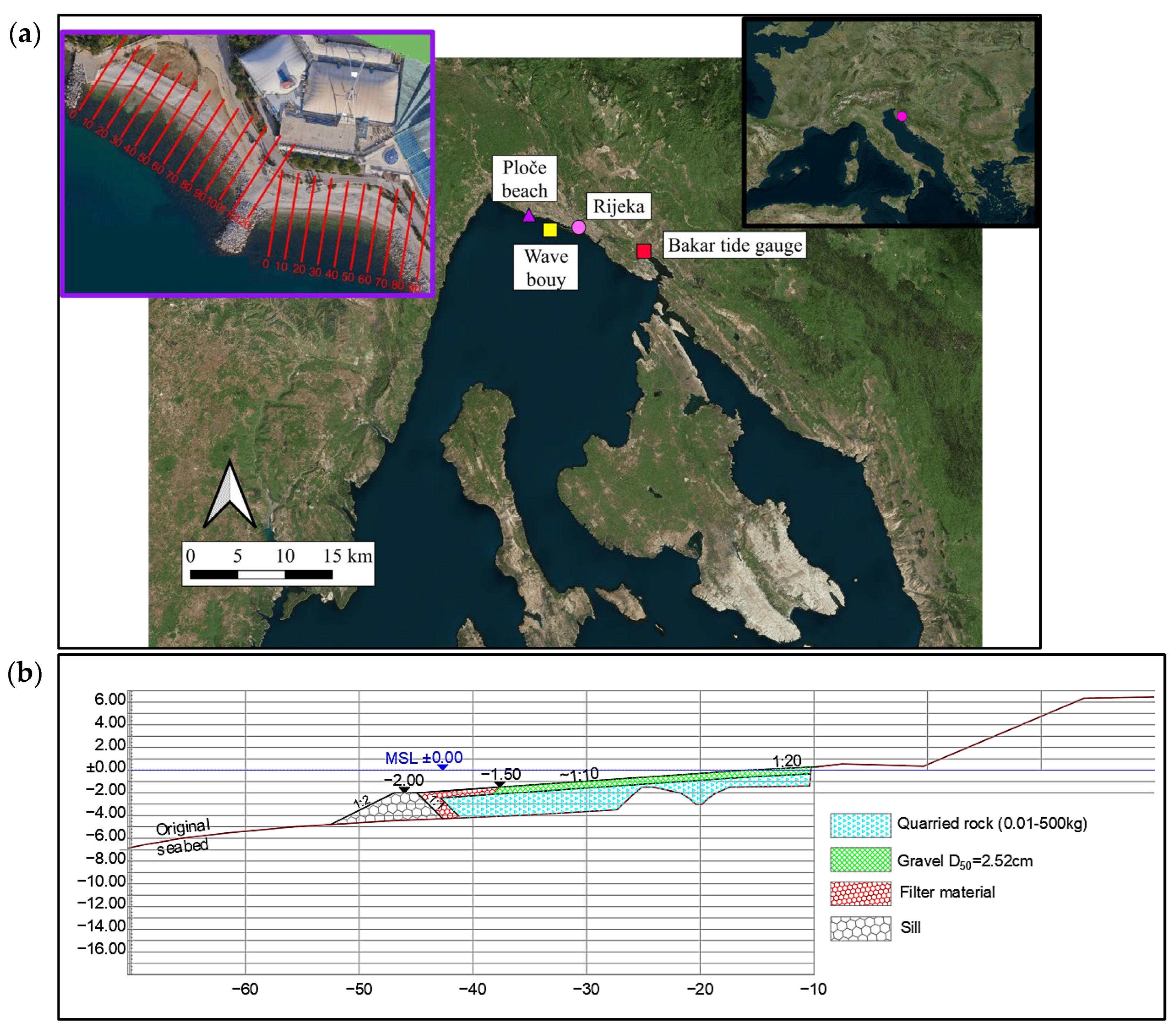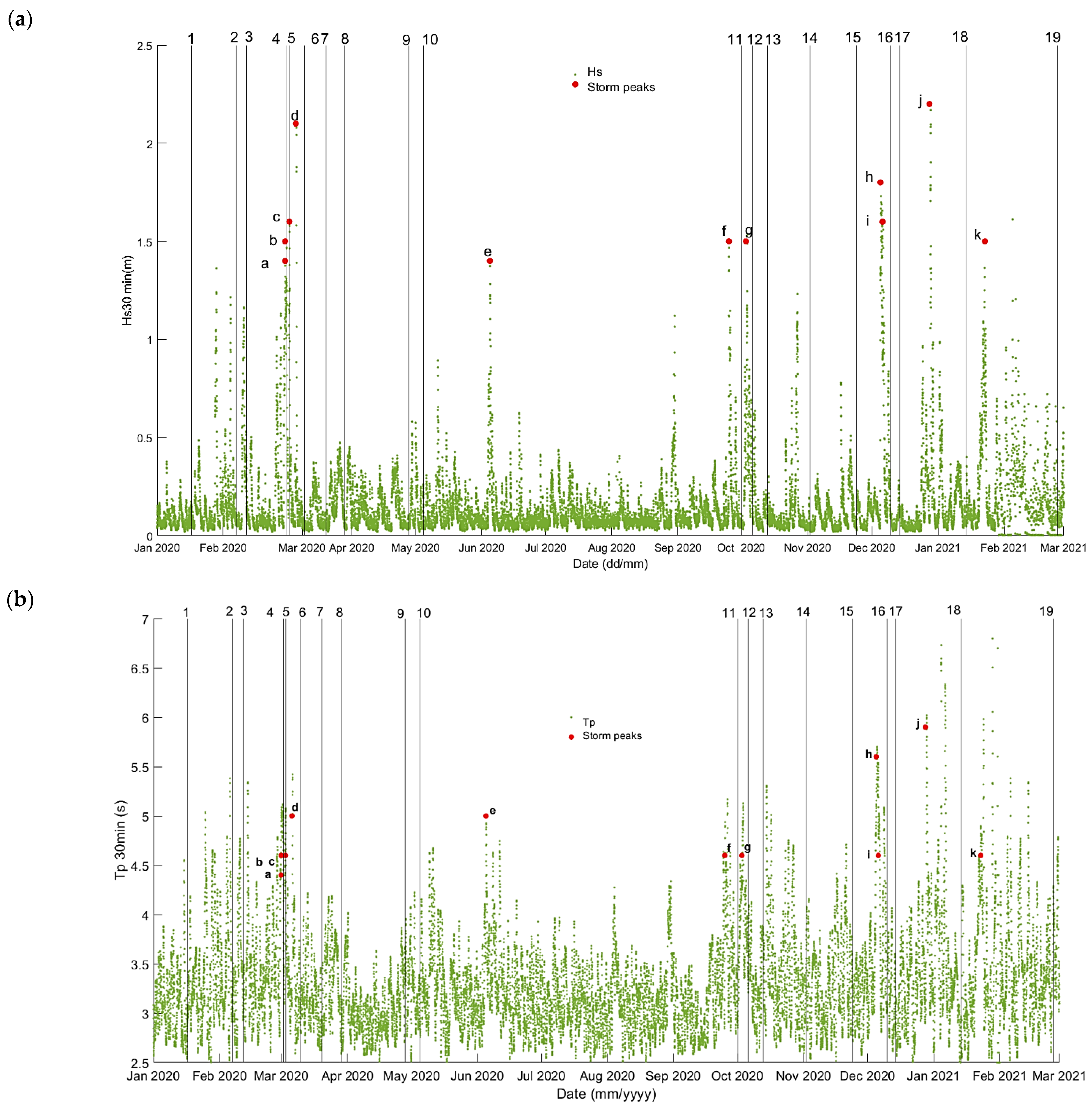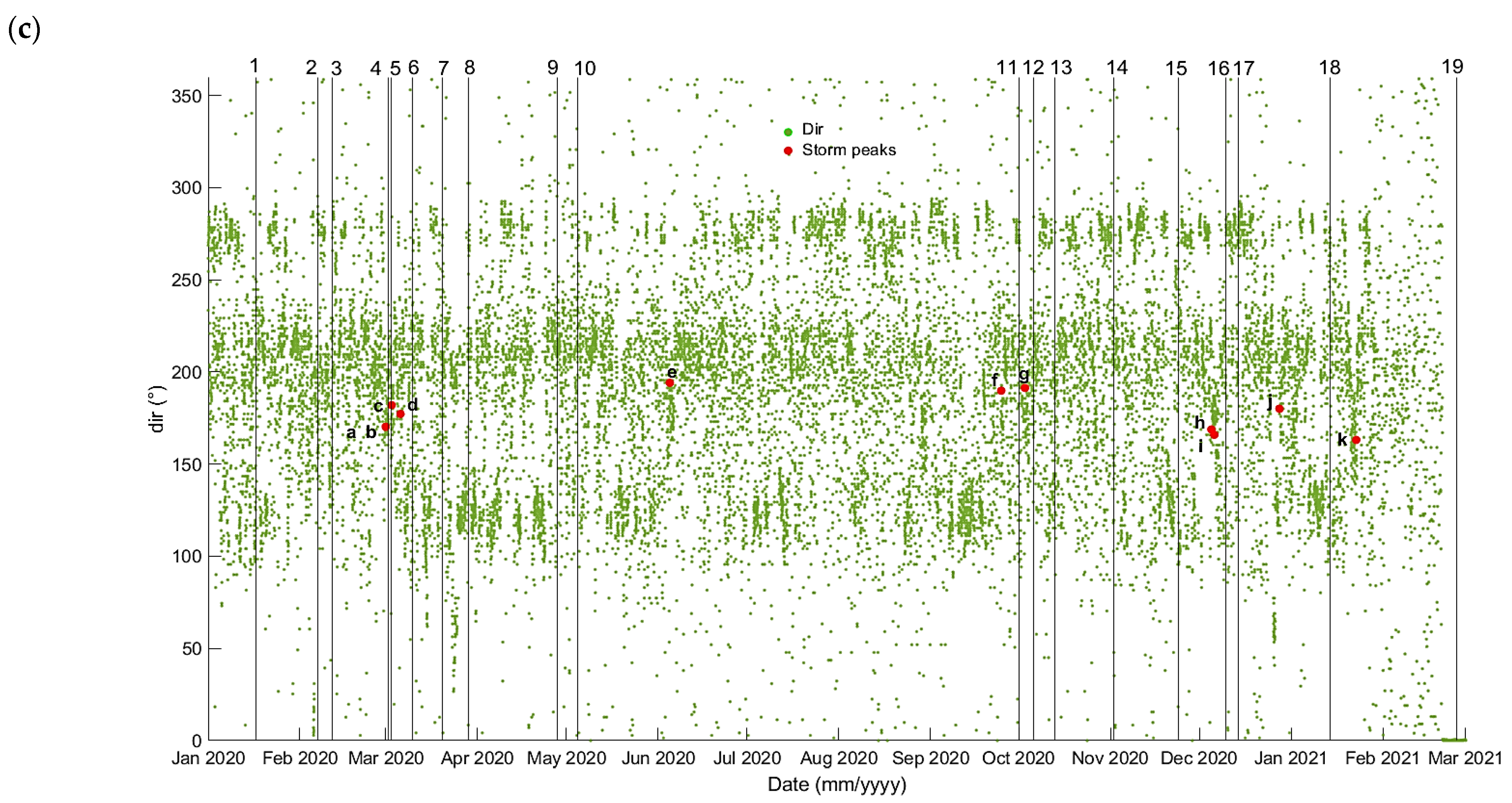This study investigates the morphodynamics of artificial gravel pocket beaches, focusing on berm formation and crest build-up processes characteristic for low to moderate wave conditions. Despite mimicking natural formations, artificial beaches require regular maintenance due to sediment shifts dominantly caused by wave action and storm surges. Structure-from-Motion (SfM) photogrammetry and UAV-based surveys were used to monitor morphological changes on the artificial gravel pocket beach Ploče (City of Rijeka). The XBeach-Gravel model, originally adapted to simulate the effects of high-energy waves, was calibrated and validated to analyze low to moderate wave dynamics on gravel pocket beaches. The calibration includes adjustments to the inertia coefficient (ci), which influences sediment transport by shear stress at the bottom; the angle of repose (ϕ), which controls avalanching and influences sediment transport on sloping beds; and the bedload transport calibration coefficient (γ), which scales the transport rates linearly. By calibrating XBeach-G for low to moderate wave conditions, this research improves the accuracy of the model for the cases of morphological responses “berm formation” and “crest build-up”.

1. Introduction

Coarse-grained beaches are coastal environments dominated by larger sediments such as gravel, pebbles, and cobbles. These beaches play a vital role in protecting coastal areas from wave run-up and storm surges [1]. Their morphodynamic evolution, referring to the changes in shape and structure over time, is influenced by natural processes such as waves, tides, and sediment transport. The Croatian Adriatic coast is known for its small gravel pocket beaches, typically located in bays surrounded by cliffs or rock formations. These pocket beaches either form naturally through wave and river erosion or are artificially constructed for recreational or protective purposes, like Ploče Beach was [2,3]. Artificial beaches are vulnerable to higher levels of sediment transport and consequently require frequent maintenance in the form of nourishment and material redistribution. This makes the artificial beach in Ploče an ideal research site, as sediment movement can be monitored almost annually. In the characteristic wave climate of the eastern Adriatic, low- to moderate-energy waves dominate, primarily leading to the formation of berms—raised ridges of sediment along the high tide line [4].

Monitoring these changes is essential for effective beach management. Structure-from-Motion (SfM) photogrammetry, using unmanned aerial vehicles (UAVs), has become an important tool in coastal monitoring [5]. This technology creates high-resolution 3D point clouds and digital elevation models (DEMs), offering precise measurements of beach morphology [6,7].

Numerical models have been developed to simulate the morphodynamics of gravel beaches. Process-based numerical models offer a more accurate approach by incorporating fundamental physical principles, providing better predictions of storm impacts and coastal changes [4,8,9,10,11]. Despite their potential, there is a significant gap in the development of these models specifically for gravel beaches due to a lack of measured data related to morphological changes. Van Gent’s [12,13] and Pedrozo-Acuña et al.’s [14] models have provided useful insights, but challenges remain in capturing all the complexities of gravel beach dynamics. Process-based models such as XBeach have been widely applied to sandy beaches. For example, Roelvink and Costas [15] coupled hydrodynamic and aeolian processes to simulate coastal dune interactions, Marino et al. [16] evaluated the effectiveness of nature-based solutions (NbSs) in mitigating storm impacts under climate change scenarios, while De Beer et al. [17] highlighted the limitations of wave-averaged modes on intermediate–reflective sandy beaches and promoted the use of wave-resolving approaches. These studies, however, were all focused on sandy beaches.

Utilizing the open-source model for sandy beaches, XBeach, Williams, J.J. [18] and Jamal, M.H. [19] extended the model to include equations for gravel transport and water infiltration and showed good agreement of these extended models with a limited number of measured results on gravel beaches and under laboratory conditions. Building on these results, McCall, R.T. [20,21] further developed a specific process-based model derived from XBeach to describe the morphodynamics of gravel beaches during storm events. The modifications and extensions of the XBeach model presented in the papers resulted in a new numerical model, XBeach-Gravel. The authors recommend calibration and validation of XBeach-G for each specific site, which is essential to ensure that model predictions match real observations. The recommended free model parameters related to sediment transport are the coefficient of inertia (ci), which influences sediment transport through shear stress at the bottom; the angle of repose (ϕ), which controls avalanching and influences sediment transport on sloping beds; the bedload transport calibration coefficient (γ), which linearly scales transport rates; and hydraulic conductivity (kx), which reflects how easily water can pass through the sediment, affecting how waves and water movement influence sediment transport and deposition [20]. To assess the predictive ability of the numerical model, McCall, R.T. [20] recommended sediment transport parameters (ci = 1.0; ϕ = 35°; γ = 0.5) for all natural gravel sites the author studied and kx estimated according to beach granulometry. However, for the BARDEX laboratory results, a higher transport coefficient γ of 1 was proposed by McCall, R.T. et al. [20]. This adjustment was justified by the fact that the river sediment used in the experiment, due to its rounded shape, exhibited greater mobility compared to marine-origin sediment typically expected on beaches [20]. Since the XBeach-G model was validated for simulating the effects of storm events on the morphodynamical response of natural beaches at significant wave heights of approximately Hs = 5 m and higher, relatively few model validations have been performed for closed seas with smaller fetches, where wave heights are lower. These issues were addressed in a study by Bogovac, T. [3], where the model calibration was performed for an artificial gravel beach, Ploče in Croatia, by varying calibration parameters in the range (γ = 0.25–1.5 and kx = 0.05–0.5) and constant parameters (ci = 1.0; ϕ = 35°). The authors modeled each storm event by utilizing a variable boundary condition (significant wave height—Hs, peak period—Tp, and tidal oscillations) and concluded that the best results according to BSS factors were obtained for kx = 0.3 m/s and γ = 0.25. The study highlighted the challenges of using variable boundary conditions in the case of pocket beaches and the 1D numerical model (XBeach-G), primarily due to difficulties in accurately simulating wave setup. In the same study, a calibration process was performed for the beach profile response of the wave flume experiments performed in [22]. The authors used constant boundary conditions (Hs, Tp) and found that the best BSS factors were acquired for parameters kx = 0.4 m/s and γ = 3, which proves the conclusions from [20] regarding larger material mobility in the wave flume.

The present study employs fixed boundary conditions (Hs, Tp, and tide) to improve the prediction accuracy of the XBeach-G model developed by Bogovac, T. [3]. The primary objective is to determine the optimal combination of calibration coefficients (ci, ϕ, and γ) for accurately describing berm formation and crest build-up, a common morphological response on Croatian beaches. Geodetic survey data from Ploče beach were analyzed to identify storms during which cross-shore sediment transport was dominant. This approach provided a solid foundation for the calibration process by establishing reliable beach profiles before and after the selected storms.

The paper first presents the monitoring approach and beach conditions in Section 2, followed by the numerical modeling setup and calibration process. The results and model performance are discussed in Section 3, while Section 4 concludes with key findings and recommendations for future work.

2. Materials and Methods

2.1. Conditions on the Artificial Beach Ploče

Ploče beach is an artificial gravel beach constructed as a part of the Kantrida swimming pool complex, built between 2008 and 2011 and located approximately 5 km west from the city of Rijeka. As a part of the complex, three rock groins were built, creating two beach cells. The new beach (Figure 1) stretches over 360 m of shoreline. An integral part of the beach is a submerged sill that retains the sediment on the beach itself and prevents its loss in depth. Both cells are filled with a quarried rock on which the surface layer of river gravel is placed. The granulometric analysis of a sample of 1087 grains collected in February 2022 on 8 different profiles perpendicular to the two beach cells gave an average grain diameter of 2.52 cm. The average grain diameters for the different profiles ranged from 2.03 cm to 3.22 cm [3].

The eastern cell of the beach is oriented to the south, and the western cell to the southwest. This orientation exposes the beach to the waves that occur in the Bay of Rijeka, with the effective wind fetch limited to about 20 km.

The incoming wave parameters were measured on a wave buoy (Datawell Waverider MkIII) moored 2.5 km southeast of the beach. Wave parameters were integrated over a 30 min period (Figure 2), giving the significant wave height, Hs; the peak period, Tp; and the direction of occurrence of the waves, DIR. A total of 11 storm events were identified based on the 99.5th percentile threshold of significant wave height data recorded at the wave buoy, corresponding to Hs = 1.26 m [5]. These events are represented by red dots in Figure 2 [5]. The directions of the associated storms fall within the range of 160–200° and cause longshore and cross-shore material transport. The data on tidal oscillations were taken from the tidal station in Bakar. The highest tide level in the observation period was 0.9 m and occurred on 8 December 2020. With a low tide of −0.34 m compared to mean sea level, the range of the tidal oscillations during this period was 1.24 m.

The morphological changes were monitored through 19 geodetic surveys conducted between 17 January 2020 and 26 February 2021. The methodology and results of these measurements are thoroughly detailed in the paper by Tadić, A. [5]. While the original study focused solely on the western cell, this paper also includes the eastern cell. Each survey involved the development of a 3D beach model following significant storms, as illustrated in Figure 2, which is numbered from 1 to 19. Figure 3 and Figure 4 depict beach elevation changes exceeding 0.05 m for the western and eastern cells, respectively. Eroded areas are represented in shades of blue and green, while sediment accumulation is indicated in shades of orange and red. The presentation omits images of UAV6&7 through UAV9&10, UAV13&14, and UAV16&17, as no storm conditions were recorded during these timeframes and these surveys are not relevant for the analyses. The beach is regularly nourished each year with new gravel, and the material is redistributed using machinery to flatten the beach surface. This process is consistently repeated each spring in preparation for the upcoming tourist season.

For this research, the same procedure was carried out on 31 January 2020, between UAVs 1 and 2, where 150 m³ of a new gravel was brought on the western cell, as shown in Figure 3. The elevation changes in this cell indicate that material was moved from the higher areas towards the toe of the beach. On the right-hand side, additional material was added, resulting in positive changes, as depicted in red. No interventions were made in the eastern cell on that date. UAV10&11 indicate another artificial intervention on both beach cells. During this intervention in May 2020, existing material was redistributed in the lower sections of the cells. Moreover, on the UAV17&18, intervention is visible on the eastern cell where the beach area was flattened in January 2021.

Western cell. After the artificial nourishment (between UAV1 and UAV2), the first few storm events (a, b, c, and d in Figure 2) transported the gravel material along the coast toward the left part of the cell, and all the eroded gravel accumulated on the left part (Figure 3), forming an equilibrium position. The right part remained bare, exposing the immobile quarried rock embankment beneath the gravel layer. In UAV5&6, most of the changes occurred in the left and central parts of the western cell due to cross-shore sediment transport only, without pronounced longshore transport. The cross-shore pattern is visible in Figure 3 after stronger storms (UAV5&6, UAV15&16, UAV17&18) where the eroded zone (green) is distributed beneath the accreted zone (red) uniformly along the beach. The rainfall that occurred on 1 and 2 March 2020, is visible on the UAV3&4 image, depicted with blue color where strong water currents eroded three deep channels in the beach body.

Eastern cell. Due to technical difficulties with the drone during the UAV15 survey, the results for UAV14&15 and UAV15&16 in the eastern cell are unavailable. However, based on the remaining data, several conclusions can be drawn. Similar to the western cell, the gravel material in the eastern cell is influenced by wave action, leading to an equilibrium position of the beach. Most of the gravel is transported toward the northeastern part of the cell, creating a stable beach form that persists under various wave and tide conditions. This stable beach form is evident in the cross-shore transport patterns observed in UAV5&6, where eroded (green) and accreted (red) zones are aligned parallel to the beach, mirroring the patterns seen in the western cell. A comparable pattern is also noted during some weaker storms, as seen in UAV3&4 and UAV18&19. It is important to highlight that beach morphology is significantly affected by the concrete wall at +1.65 m.a.s., which acts as a barrier between the gravel and the adjacent walkway.

One of the objectives of this study is to identify beach zones characterized by stable cross-shore processes, which will be utilized for calibrating the numerical 1D model (XBeach-Gravel). Stable cross-shore beach zones are defined as areas with minimal long-shore transport between two consecutive geodetic surveys. To achieve this, longshore analyses are performed using erosion-accretion diagrams, as illustrated in Figure 5. Each green column in the graph indicates the specific volume (m³/m′) of material eroded between two surveys in the profile, determined by the cross-shore distance (Figure 1a). The volume of material that has accreted is represented by the red columns on the same profile. The height of each column reflects the intensity of the change, allowing for direct visual comparison across the profile. When the red and green columns are approximately equal for a characteristic profile or zone, it suggests that dominant cross-shore transport is observed between the two successive surveys, and there is no significant net gain or loss of material in the longshore direction. These zones are indicative of morphodynamic equilibrium and are thus suitable for 1D cross-shore numerical modeling. Conversely, when there is a clear imbalance, such as a predominance of either red or green columns, this indicates the dominance of longshore transport, often triggered by structural interventions or specific wave conditions. For example, this can be observed in UAV3&4 for profiles 60–100, where evident longshore redistribution of the material is present. Profiles within dominant cross-shore transport zones are deemed suitable for 1D numerical modeling, as discussed in the subsequent Section 2.2.

Figure 5 highlights only the stable cross-shore zones identified in Figure 3 and Figure 4, while zones affected by longshore transport, mainly due to the influence of the rubble mound groins and the concrete wall of the walkway, are shaded in gray. These shaded areas represent locations where lateral movement of sediment is prominent and thus unsuitable for simplified 1D modeling. In certain areas, a clear inequality between accretion and erosion is evident. For instance, in the case of UAV4&5 for the western cell (Figure 5), additional accretion is observed in profiles from the 20th to the 50th meter, attributed to the filling of channels created by rainfall on 1 and 2 March 2020. Similarly, in the cases of UAV15&16 for the western cell and UAV17&18 for the eastern cell, longshore transport is noticeable toward the left and right sides, respectively. However, the longshore transport observed in eastern cell for UAV17&18 was carried out by machinery in the scope of the regular beach maintenance. Given that all data collected for this study were obtained under “natural conditions,” some deviations are acceptable. Profiles suitable for 1D numerical modeling were selected with the aim of avoiding processes that do not meet the assumptions of dominant cross-shore material transport. The erosion-accretion diagrams, therefore, serve not only as a tool for quantifying volumetric changes but also for interpreting spatial sediment transport patterns. Their integration into the profile selection process ensures that the numerical simulations are grounded in morphologically consistent and physically meaningful inputs.

Table 1. Surveys and profiles selected for the calibration and validation of the XBG model along with relevant storm input parameters for XBG (bold values).

Survey	Storm Event	Start of Storm	End of Storm	Hs,max [m]	Tp [s]	Dir [°]	Tide max [m]	Rc/Hmo	Morphodynamic Response	Selected Profiles for XBG Calibration in Western Cell [m]	Selected Profiles for XBG Validation in Eastern Cell [m]	Estimated Wave Setup in Western and Eastern Cell Wsadded [m]
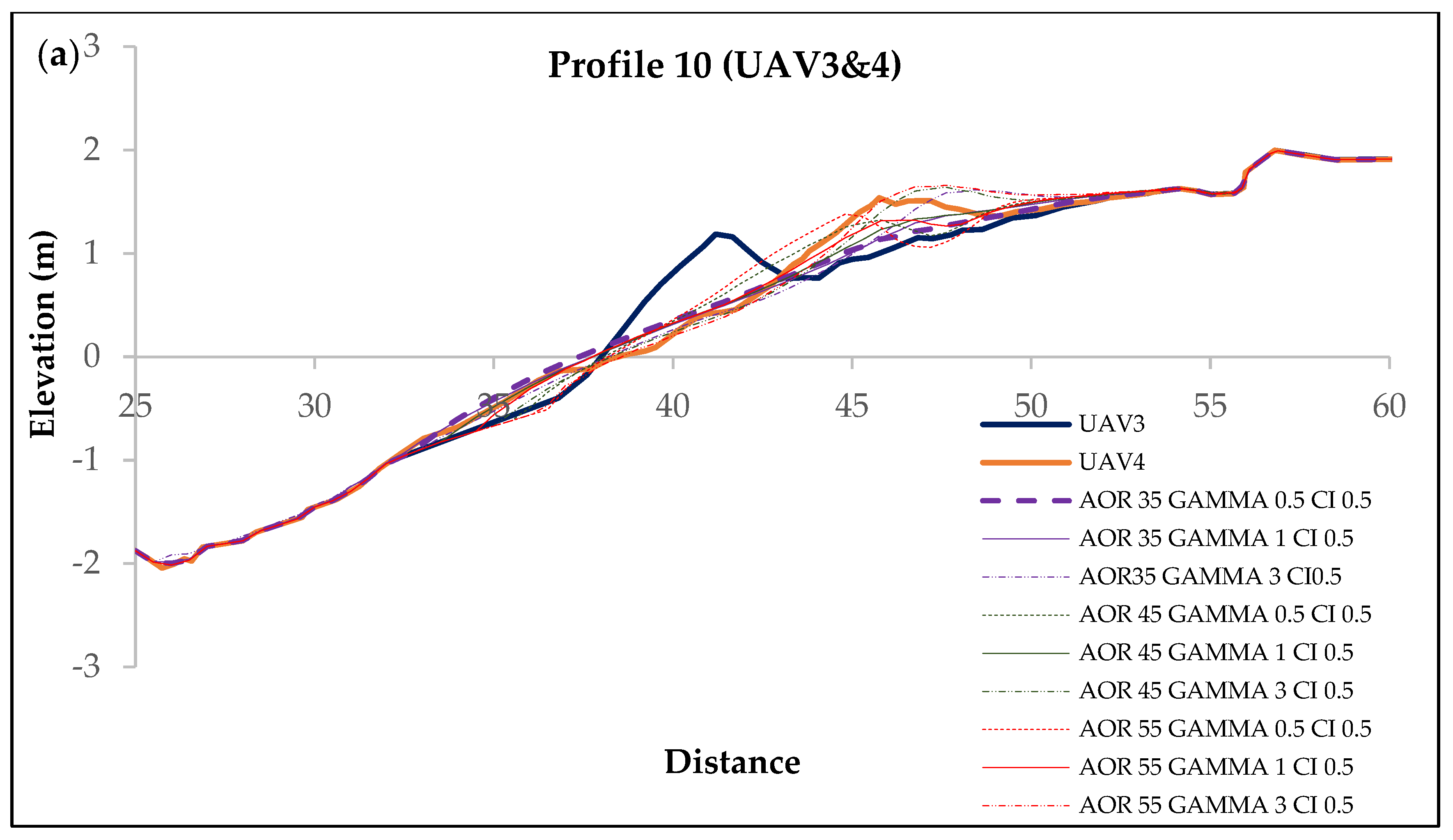
UAV3&4	a & b	1 March 2020 00:34	1 March 2020 04:09	1.4	4.4	170.2	0.40	1.18	Berm formation	10	70	0.44
		1 March 2020 14:29	1 March 2020 20:32	1.5	4.6	170.2	0.32	1.10
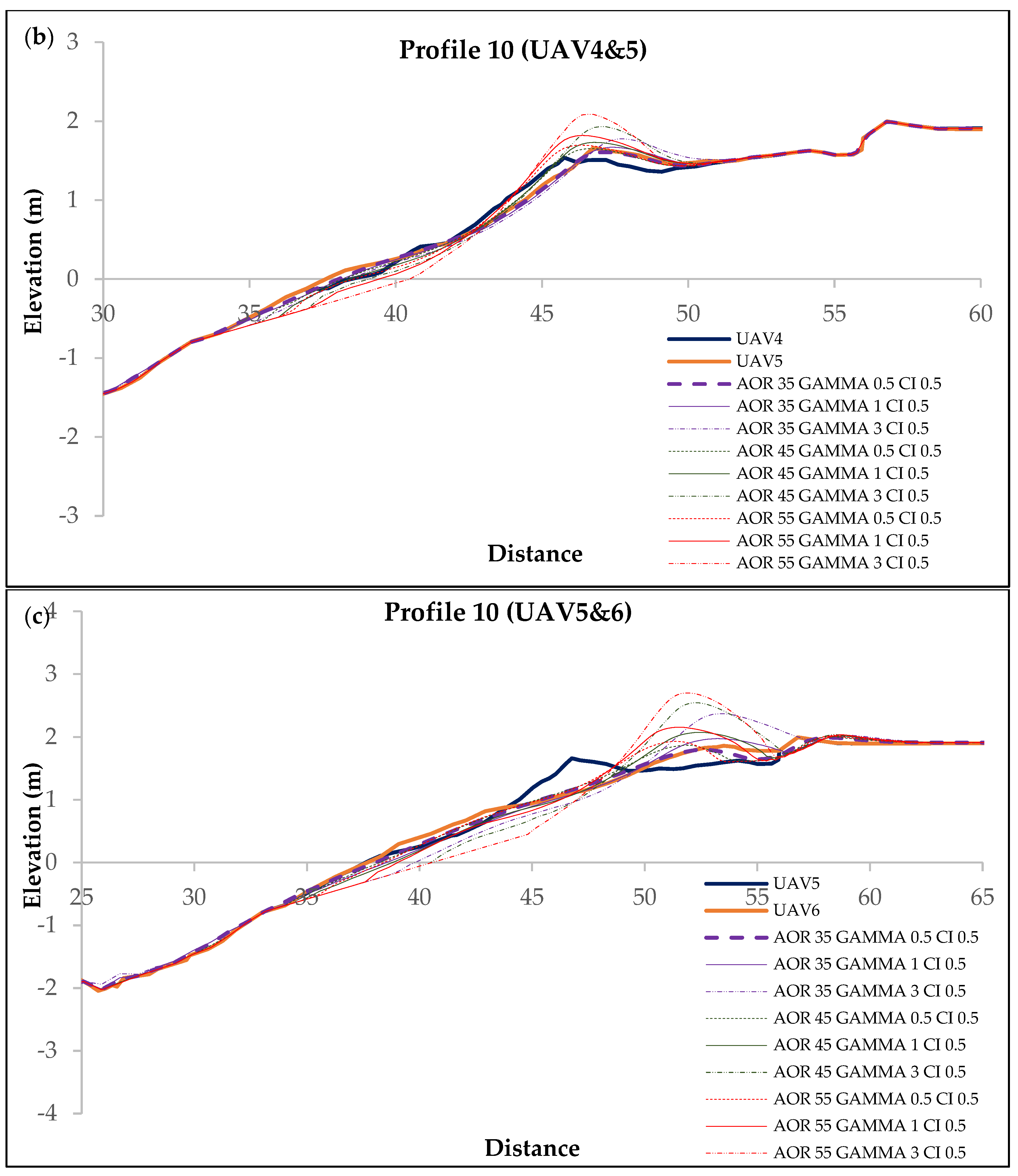
UAV4&5	c	3 March 2020 00:15	3 March 2020 02:28	1.6	4.6	182.8	0.57	1.03	Berm formation	10	70	0.16
UAV5&6	d	6 March 2020 05:46	6 March 2020 08:41	2.1	5	177.2	0.57	0.79	Crest build-up	10	70	0.53
UAV10&11	e & f	5 June 2020 00:21	5 June 2020 01:53	1.4	5	194.1	0.00	1.18	/	No profile selection due to intervention on the beach		/
		25 September 2020 01:18	25 September 2020 03:41	1.5	4.6	189.8	0.29	1.10	/			/
UAV11&12	g	3 October 2020 15:01	3 October 2020 16:18	1.5	4.6	191.3	0.46	1.10	/	No profile selection due to large tidal variations		/
UAV12&13	/	below storm conditions		0.64	3.52	203.9	0.49	2.58	Berm formation	20	70	0.1
UAV14&15	/	below storm conditions		0.8	3.68	183.4	0.071	2.06	Berm formation	10	missing UAV15	0.1
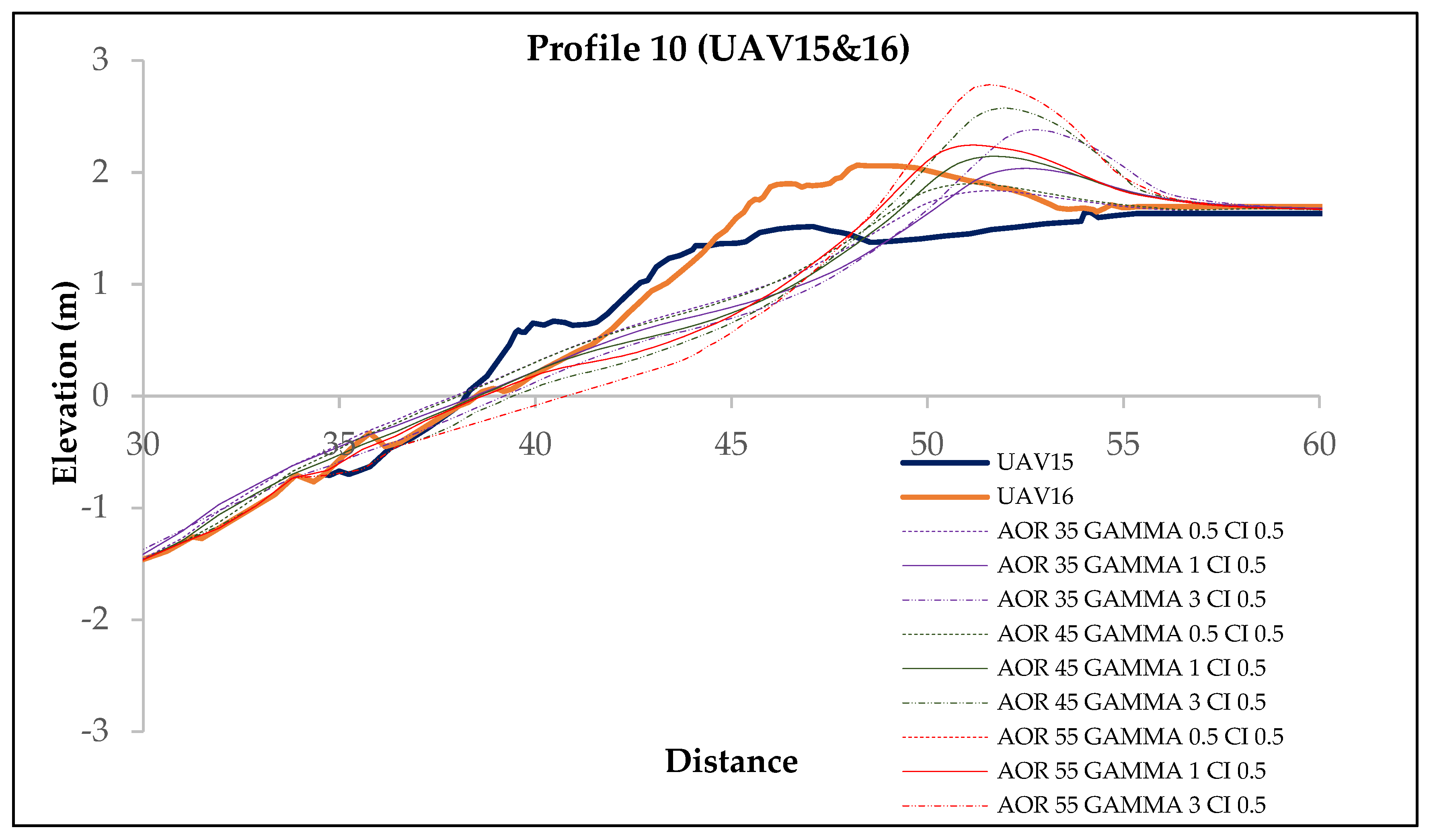
UAV15&16	h & i	5 December 2020 00:53	5 December 2020 22:58	1.8	5.6	168.8	0.61	0.92	Crest build-up	10	missing UAV15	0.45
		6 December 2020 08:31	6 December 2020 09:43	1.6	4.6	165.9	0.71	1.03				/
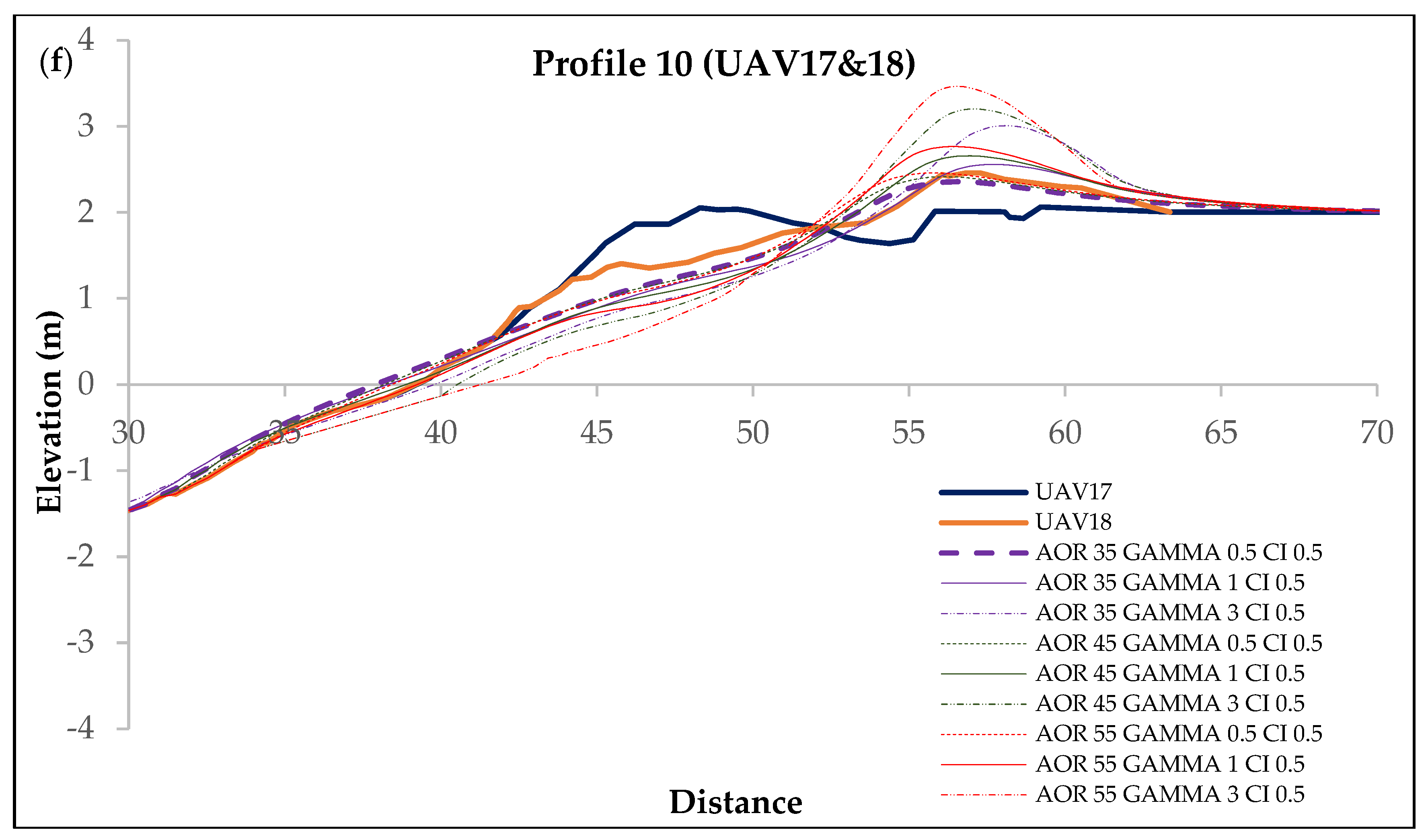
UAV17&18	j	28 December 2020 10:43	28 December 2020 20:08	2.2	5.9	180	0.69	0.75	Crest build-up	10	intervention on the beach	0.81
UAV18&19	k	23 January 2021 00:03	23 January 2021 01:35	1.5	4.6	163.1	0.53	1.10	/	No profile selection due to the measurement error		/

outlines the profiles selected for 1D numerical modeling (XBG), along with corresponding storm data and tide information. The surveys UAV10&11, UAV11&12, UAV14&15, UAV15&16, UAV17&18, and UAV18&19 have limited applicability and are not utilized at all due to the constraints highlighted in Table 1. Consequently, seven surveys are selected for XBG calibration, which will be conducted in profiles at 10 m and 20 m in the western cell. For the model validation, four profiles are selected at 70 m in the eastern cell, as these profiles exhibit the lowest levels of longshore transport (Figure 5).

2.2. Numerical Model XBeach-Gravel and Model Setup

Details on the extended capabilities of an existing open-source, process-based hydrodynamic model for gravel coasts (XBeach-G) can be found in the studies by McCall, R.T. [20,21].

The findings in the study Powell, K.A. [23] indicated that 3000 waves were sufficient to establish a state of dynamic equilibrium, after which no further changes in the beach profile were expected. To optimize computational efficiency, the simulation duration was determined using Equation (1).

$$t={\displaystyle \frac{Tp}{1.1}}\times n$$

(1)

where Tp (s) is the peak period of incoming waves, t (s) is the duration of each simulation, and n corresponds to the number of waves required to reach equilibrium, which is 3000. The mean wave period in the previous equation is estimated as Tm = Tp/1.1 according to Goda, Y. [24]. The significant wave heights used in numerical simulations were selected as the maximum values recorded between two field measurements (UAVs), while the Tp value corresponded to the peak period associated with the maximum significant wave height (red dots in Figure 2). Since most beach changes occur between −1 and 2 m in elevation along the profile, the numerical model boundary was set at a depth of −5 m (corresponding to the position of the submerged sill’s toe) to ensure accurate simulation of incoming wave heights. The position of the non-erodible layer on the beach was also incorporated into the simulation, as presented in Figure 6. This layer marks the transition where quarried rock begins, preventing further material erosion due to its compact composition. The model simulates only the movement of gravel within the uppermost layer of the beach structure, while the quarried rock layer, sill, and seabed remain motionless. To calibrate the model, free model parameters related to sediment transport were varied: the coefficient of inertia (ci), the calibration coefficient for bedload transport (γ), and the angle of repose (ϕ). The aim was to determine the combination of these two parameters that leads to a Brier skill score (BSS) of 1. Inertia coefficients (ci) of 0.5, 1, and 2, along with bed load transport coefficients of (γ) 0.5, 1, and 3 were utilized in the calibration process, while the angle of repose was varied at 35°, 45°, and 55°.

In addition to the previously mentioned model parameters and the wave parameters listed in Table 1, fixed values for the hydraulic conductivity (kx) of 0.4 m/s and the mean grain size (D50) of 2.52 cm were used in all simulations, as recommended in the earlier study by Bogovac, T. [3] on Ploče beach. In addition, the profile parameters were set with a minimum grid size of 0.1 m, a maximum grid size of 0.5 m, and a minimum of 40 points per wavelength. The wave parameters were set with a unimodal JONSWAP spectrum for all waves, while the tidal parameters included a variable back-boundary water level. Van Rijn, L.C.’s [25] formula was used for the sediment transport calculations.

In the case of pocket beaches, larger values of wave setup (WS_added) are expected and compared to straight beaches due to their enclosed shape which disables water introduced by waves to be removed out [25]. XBeach-Gravel, as a 1D model, computes wave transformation perpendicular to a straight coastline and does not account for the curvature of pocket beach shorelines and consequently increased wave setup, as noted by Bogovac, T. [3]. To address this limitation in the simulations, the tidal level in the model was adjusted by adding the predicted wave setup (WS_added), resulting in (Tide_numeric = Tide_max + WS_added). The values of estimated WS_added are presented in Table 1.

2.3. Brier Skill Score

The Brier skill score (BSS) is used to quantify the ability of a model to predict actual measured changes in the beach profile. This metric is commonly used in numerical coastal modeling [20,26]. It is calculated based on the absolute difference between the modeled and measured profile changes at each point, with the instrumental error subtracted from this value. If the resulting value is negative, i.e., if the difference between the model and the measurements is smaller than the instrumental error, it is set to 0. The resulting value is called the absolute prediction error, denoted by |ϵΔξ|, and is calculated using Equation (1) for each profile point. In this study, an instrumental error of 0.1 m was assumed, based on the precision of the instrument used for the topographic survey on Ploče beach.

$$\left|{ϵ}_{\mathsf{\Delta }\xi }\right|=\max \left(\left|\mathsf{\Delta }{\xi }_{modelled}-\mathsf{\Delta }{\xi }_{measured}\right|-{ϵ}_0,0\right)$$

(2)

It is important to emphasize that the profile change is determined as the difference between the initial and final profile after a storm event both in the model and on the actual beach. It follows from Equation (3) that the BSS value can be less than or equal to 1. The initial profile is the same for both the model and the beach, as it was measured before the storm event. The final profile is measured onsite and compared with the profile generated by the model. The aim of the calibration is to find model parameters that lead to a modeled beach profile after a storm that is close to the measured profile, considering the measurement error.

$$BSS=1-{\displaystyle \frac{\frac{1}{n}{\sum }_{i=1}^n{\left|{ϵ}_{\mathsf{\Delta }\xi }\right|}_i^2}{\frac{1}{N}{\sum }_{i=1}^n{\left({\mathsf{\Delta }\xi }_{i,measured}\right)}_i^2}}$$

(3)

After determining the prediction error of the model (|ϵΔξ|) using Equation (2), the Brier skill score can be calculated using Equation (3), where the summation applies to all profile points. If BSS equals 1, this means that |ϵΔξ| is 0 at each point, indicating excellent agreement between the model and the measurements within instrumental accuracy. If BSS is 0, this means that the model predicts no changes between the initial and final profiles. A BSS value between 0 and 1 reflects improved model performance in approximating the measured changes, with the different values in this range classified according to

Table 2. Classification of Brier skill score by Van Rijn, L.C. [26].

Brier Skill Score	Interpretation
0.8–1	Excellent
0.6–0.8	Good
0.3–0.6	Fair
0–0.3	Poor
<0	Bad

. A negative BSS value indicates that the model performs worse than the base case where no profile changes are predicted.

3. Results and Discussion

A total of 189 simulations were performed for seven selected storm events (Table 1), varying the three parameters mentioned above. The optimal parameter combination was selected based on the highest average BSS value for all storm events. The resulting BSS values in relation to the inertia coefficient, bed load transport coefficient, and angle of repose are shown in

Table 3. (a) Brier skill score values for calibration of 7 storm events for different angles of repose (ϕ), bed load transport coefficients (γ), and coefficient of inertia (ci) of 0.5. (b) Brier skill score values for calibration of 7 storm events for different angles of repose (ϕ), bed load transport coefficients (γ), and coefficient of inertia (ci) of 1. (c) Brier skill score values for calibration of 7 storm events for different angles of repose (ϕ), bed load transport coefficients (γ), and coefficient of inertia (ci) of 2. Storm events selected for BSS calculation are highlighted as shaded rows.

(a)
BSS	ϕ 35°, γ 0.5	ϕ 35°, γ 1	ϕ 35°, γ 3	ϕ 45°, γ 0.5	ϕ 45°, γ 1	ϕ 45°, γ 3	ϕ 55°, γ 0.5	ϕ 55°, γ 1	ϕ 55°, γ 3
UAV3&4	0.86	0.89	0.87	0.91	0.93	0.95	0.81	0.95	0.94
UAV4&5	0.84	0.83	0.51	0.66	0.42	−0.77	−0.06	−1.34	−4.68
UAV5&6	0.92	0.83	−0.83	0.80	0.58	−2.32	0.60	−0.02	−4.60
UAV12&13	0.93	0.96	0.95	0.85	0.73	0.32	0.63	0.20	−0.58
UAV14&15	0.61	0.65	0.65	0.87	0.92	0.79	0.96	0.88	0.60
UAV15&16	−0.64	−1.32	−2.01	−0.54	−1.18	−1.97	−1.70	−1.04	−2.60
UAV17&18	0.76	0.54	−0.39	0.75	0.45	−1.47	0.70	0.15	−3.67
Average BSS	0.82	0.76	0.29	0.81	0.67	−0.42	0.61	0.14	−2.00
(b)
BSS	ϕ 35°, γ 0.5	ϕ 35°, γ 1	ϕ 35°, γ 3	ϕ 45°, γ 0.5	ϕ 45°, γ 1	ϕ 45°, γ 3	ϕ 55°, γ 0.5	ϕ 55°, γ	ϕ 55°, γ 3
UAV3&4	0.95	0.95	0.89	0.96	0.93	0.81	0.93	0.86	0.62
UAV4&5	0.60	0.51	0.16	−0.13	−0.45	−1.49	−1.26	−1.96	−4.75
UAV5&6	0.38	−0.08	−1.48	−0.20	−0.95	−2.93	−0.72	−2.03	−5.13
UAV12&13	0.91	0.85	0.82	0.74	0.48	0.28	0.36	−0.08	−0.58
UAV14&15	0.79	0.78	0.73	0.91	0.90	0.85	0.95	0.88	0.73
UAV15&16	−0.14	−0.60	−1.21	0.00	−0.62	−1.56	0.05	−0.68	−2.55
UAV17&18	0.63	0.28	−1.03	0.54	−0.26	−2.61	0.28	−1.21	−4.60
Average BSS	0.77	0.67	0.32	0.60	0.32	−0.43	0.25	−0.30	−1.72
(c)
BSS	ϕ 35°, γ 0.5	ϕ 35°, γ 1	ϕ 35°, γ 3	ϕ 45°, γ 0.5	ϕ 45°, γ 1	ϕ 45°, γ 3	ϕ 55°, γ 0.5	ϕ 55°, γ 1	ϕ 55°, γ 3
UAV3&4	0.95	0.94	0.90	0.90	0.91	0.85	0.79	0.83	0.73
UAV4&5	−0.25	−0.28	−0.47	0.66	−1.11	−1.90	−2.05	−2.77	−4.14
UAV5&6	−0.52	−1.01	−1.56	−1.42	−2.02	−3.10	−2.05	−2.90	−4.56
UAV12&13	0.78	0.78	0.88	0.34	0.34	0.34	−0.08	−0.15	−0.35
UAV14&15	0.85	0.86	0.78	0.92	0.92	0.90	0.93	0.92	0.78
UAV15&16	0.17	−0.34	−0.38	0.01	−0.55	−1.05	−0.17	−0.94	−0.60
UAV17&18	0.02	−0.90	−1.37	−0.93	−0.93	−1.79	−1.63	−2.67	−3.86
Average BSS	0.31	0.07	−0.14	0.08	−0.32	−0.78	−0.68	−1.12	−1.90

a–c. When calculating the average BSS values for the twenty-seven different parameter combinations (ϕ 35°/45°/55°, γ 0.5/1/3, and ci 0.5/1/2), storm event UAV15&16 (Figure A2, Appendix A) was excluded from the analysis due to the longshore sediment transport effect, as described in Section 2.

For the combination (ϕ 35°, γ 0.5, and ci 0.5) which resulted in the highest average BSS value of 0.82, all storm events had BSS values ranging from “good” to “excellent” (0.6–1.0, Table 3a shaded rows). An increase in the bed load transport coefficient γ to 1 and 3 led to a deterioration in model performance, with the average BSS values dropping to 0.76 and 0.29, respectively. Similarly, for the parameter combination ϕ 45° γ 0.5, the performance of the model remained “excellent” with a BSS value of 0.81. However, for ϕ 45° γ 1 and ϕ 45° γ 3, the model performance further deteriorated compared to that of ϕ 35°, with average BSS values declining to 0.67 and −0.42, respectively. A significant decrease was observed for ϕ 55° over all bed load transport coefficients (γ 0.5, γ 1, and γ 3), with the average BSS values falling to 0.61, 0.14, and −2.00, respectively. Using the same procedure for inertia coefficients ci of 1 and 2, a decrease in the average BSS values was observed (Table 3b,c). With an angle of repose of ϕ 35° and bed load transport coefficients of γ 0.5 and γ 1, the average BSS values remained in the “good” range according to the Van Rijn classification (0.77 and 0.67 “row Average BSS” in Table 3b). However, all other parameter combinations had BSS values ranging from “bad” to “poor” and are therefore not considered.

XBeach-G calibration results can be found in the Appendix (Figure A1a–f). The highest average BSS value of 0.82 implies that the parameter combination ϕ 35°, γ 0.5, and ci 0.5 allows the model to give the best description of changes in the profile of the artificial pocket beach in Ploče. However, a satisfactory model performance was also achieved by other parameter combinations, such as (ϕ 45°, γ 0.5, ci 0.5) and (ϕ 35°, γ 0.5, ci 1), with average BSS values of 0.81 and 0.77 in Table 3a,b. Further combinations result in additional reductions in the average BSS.

With a higher ϕ, a steeper slope could be achieved, while a higher γ results in a higher berm elevation. By combining these two parameters, almost any shape of the berm could be reached, as can be seen in Figure A1a–f.

To validate the calibrated model, four storm events were simulated in the eastern part of Ploče beach (Figure 1a). The validation was performed for the storm events UAV3&4, UAV4&5, UAV5&6, and UAV12&13. Storm events UAV10&11, UAV11&12, UAV14&15, UAV15&16, UAV17&18, and UAV18&19 were excluded due to the reasons noted in Table 1. Profile 70 was chosen as the reference profile on the eastern part of the coast, as it exhibits the lowest level of longshore transport. For the simulation of the above events, the parameters determined as the best ones during calibration were used: (ϕ 35°, γ 0.5 and ci 0.5), (ϕ 45°, γ 0.5, ci 0.5), and (ϕ 35°, γ 0.5, ci 1). Other parameters, hydraulic conductivity kx and median grain size Dn50, were taken from a previous calibration process. The model results are shown in Figure 7 with the corresponding BSS values in

Table 4. Brier skill score values for validation of 3 storm events for different angles of repose (ϕ), bed load transport coefficients (γ), and coefficients of inertia (ci).

BSS	ϕ 35° γ 0.5 ci 0.5	ϕ 35° γ 0.5 ci 1	ϕ 45° γ 0.5 ci 0.5
UAV3&4	0.69	0.89	0.87
UAV4&5	−0.33	0.63	−0.08
UAV5&6	0.93	0.79	0.85
UAV12&13	0.93	0.48	0.86
Average	0.56	0.70	0.63

. The model generally provides an accurate representation of the berm position and height, as well as the lower beach profile, based on visual assessment for all validation cases.

Regarding the BSS values, there is an obvious drop in performance for UAV4&5 (ϕ 35° γ 0.5 ci 0.5) and (ϕ 45° γ 0.5 ci 0.5) with scores −0.33 and −0.08, both classified as “bad” performance. The model has poor prediction in the lower part of the profile which naturally occurred during the lower tidal levels of the storm (UAV5) and were not incorporated in the numerical model. This case highlights the challenges of using geodetic data from real conditions (e.g., Ploče beach) to calibrate a 1D numerical model with assumed constant boundary conditions (wave parameters and tidal oscillations).

Despite these limitations, the numerical model can reproduce morphological changes within the profile “fairly” to “excellently,” accurately capturing the height and position of the berm. However, it has reduced accuracy in describing the lower part of the profile. The presented model setup is suitable for theoretical investigations of pocket beach morphological response but cannot account for variable boundary conditions and longshore transport. These processes can only be captured using a full 2D process-based numerical model, which would provide a more comprehensive simulation by also incorporating the wave setup effects.

4. Conclusions

This study confirms the suitability of the numerical model XBeach-Gravel for the simulation of the morphodynamic behavior of artificial pocket gravel beaches under moderate to low wave conditions, as they are characteristic for the eastern Adriatic Sea. Using detailed geodetic data collected at Ploče beach, including 19 UAV-based surveys, the research focused on identifying stable cross-shore transport zones to calibrate the 1D model and better understand the processes of berm formation and crest build-up.

The calibration of the model was performed on profiles of the western beach cell using seven selected storm events with significant wave heights (Hs) between 0.64 and 2.2 m and peak wave periods (Tp) between 3.5 and 5.9 s. The most accurate results were obtained with an inertia coefficient (ci) of 0.5, bed load transport coefficient (γ) of 0.5, and an angle of repose (ϕ) of 35°, resulting in an average Brier skill score (BSS) of 0.82, which was rated as “excellent” according to Van Rijn’s assessment framework. With these parameters, the model was able to reliably reproduce the main morphological changes, including the erosion of the lower beach profile and the development of berms in the upper sections after storm events. As mentioned earlier, similar challenges were addressed in the study by Bogovac, T. [3], where the calibration of the XBeach-G model for Ploče Beach was performed by adjusting selected calibration parameters within certain ranges (γ = 0.25–1.5 and kx = 0.05–0.5), while others were held constant (ci = 1.0; ϕ = 35°). In that study [3], individual storm events were simulated with time-varying boundary conditions, including significant wave height (Hs), peak wave period (Tp), and tidal variations, with model calibration based on two storm events. The highest Brier skill score (BSS) values were obtained with kx = 0.3 m/s and γ = 0.25, highlighting the inherent difficulties in applying variable boundary conditions in one-dimensional numerical modeling of pocket beaches, particularly due to the challenges associated with accurately reproducing the wave setup. In the present study, the calibration approach was extended to seven rather than two storm events, allowing for a more comprehensive validation of model performance over a wider range of hydrodynamic conditions. In addition, the angle of repose (ϕ) was introduced as a free calibration parameter to improve model accuracy by better capturing the natural slope stability properties of coarse-grained sediments. Furthermore, the sensitivity of the XBeach-G model to variations in the inertia coefficient (ci) was also evaluated. In contrast to the approach in [3], where variable boundary conditions were used, constant boundary conditions (Hs, Tp) were used in this study for several reasons. First, the use of constant conditions simplifies the system and allows for a clearer interpretation of the morphodynamic response of the beach under specific, controlled wave and tidal forcing. Secondly, constant boundary conditions reduce computational effort, leading to faster and more numerically stable simulations by avoiding the complexities associated with rapidly fluctuating input parameters. Furthermore, to evaluate the influence of different wave heights and periods on beach erosion, constant boundary conditions facilitate clearer comparative analyzes by minimizing the overlapping effects of multiple changing variables.

Validation of the model on the eastern part of the beach was performed using four additional storm events, supporting the model’s ability to simulate real beach responses in less energetic wave climates. However, the results also revealed certain limitations, particularly in simulating the lower beach profile, which in nature is influenced by waves at lower tidal levels, the effects of longshore transport, and the accurate representation of wave setup in pocket beach environments.

Overall, the study shows that although XBeach-Gravel was originally developed for gravel beaches exposed to high-energy wave conditions, it can be successfully applied to artificial pocket beaches exposed to moderate to low wave conditions. Its ability to simulate sediment transport and profile development with satisfactory accuracy makes it a valuable tool for improving the research and management of artificial gravel beaches. This includes optimizing remediation strategies, optimizing design of the new beaches, predicting cross-shore sediment redistribution, and improving the long-term resilience of coastal infrastructures.

References

- Bujak, D.; Ilic, S.; Miličević, H.; Carević, D. Wave Runup Prediction and Alongshore Variability on a Pocket Gravel Beach under Fetch-Limited Wave Conditions. J. Mar. Sci. Eng. 2023, 11, 614. [Google Scholar] [CrossRef]
- Anthony, E.J.; Marriner, N.; Morhange, C. Human Influence and the Changing Geomorphology of Mediterranean Deltas and Coasts over the Last 6000 Years: From Progradation to Destruction Phase? Earth Sci. Rev. 2014, 139, 336–361. [Google Scholar] [CrossRef]
- Bogovac, T.; Carević, D.; Bujak, D.; Miličević, H. Application of the XBeach-Gravel Model for the Case of East Adriatic Sea-Wave Conditions. J. Mar. Sci. Eng. 2023, 11, 680. [Google Scholar] [CrossRef]
- Van Rijn, L.C. Prediction of Dune Erosion Due to Storms. Coast. Eng. 2009, 56, 441–457. [Google Scholar] [CrossRef]
- Tadić, A.; Ružić, I.; Krvavica, N.; Ilić, S. Post-Nourishment Changes of an Artificial Gravel Pocket Beach 2 Using UAV Imagery. J. Mar. Sci. Eng. 2021, 10, 358. [Google Scholar] [CrossRef]
- James, M.R.; Robson, S. Straightforward Reconstruction of 3D Surfaces and Topography with a Camera: Accuracy and Geoscience Application. J. Geophys. Res. Earth Surf. 2012, 117, F03017. [Google Scholar] [CrossRef]
- Westoby, M.J.; Brasington, J.; Glasser, N.F.; Hambrey, M.J.; Reynolds, J.M. “Structure-from-Motion” Photogrammetry: A Low-Cost, Effective Tool for Geoscience Applications. Geomorphology 2012, 179, 300–314. [Google Scholar] [CrossRef]
- Tuan, T.Q.; Verhagen, H.J.; Visser, P.; Stive, M. Numerical Modeling of Wave Overwash on Low-Crested Sand Barriers; World Scientific Pub Co Pte Ltd.: Singapore, 2007; pp. 2831–2843. [Google Scholar]
- Roelvink, D.; Reniers, A.; van Dongeren, A.; van Thiel de Vries, J.; McCall, R.; Lescinski, J. Modelling Storm Impacts on Beaches, Dunes and Barrier Islands. Coast. Eng. 2009, 56, 1133–1152. [Google Scholar] [CrossRef]
- Van Thiel de Vries, J.S.M. Dune Erosion During Storm Surges; Delft University of Technology: Delft, The Netherlands, 2009. [Google Scholar]
- Johnson, B.; Grzegorzewski, A. Modeling Nearshore Morphologic Evolution of Ship Island During Hurricane Katrina. In Proceedings of the Coastal Sediments; World Scientific: Singapore, 2011; pp. 1797–1810. [Google Scholar]
- Van Gent, M.R.A. Wave Interaction with Berm Breakwaters. J. Waterw. Port. Coast. Ocean. Eng. 1995, 121, 229–238. [Google Scholar] [CrossRef]
- Van Gent, M.R.A. Numerical Modelling of Wave Interaction with Dynamically Stable Structures. In Coastal Engineering 1996; ASCE Library: Reston, VA, USA, 2015. [Google Scholar]
- Roelvink, D.; Costas, S. Coupling nearshore and aeolian processes: XBeach and Duna process-based models. Environ. Model. Softw. 2019, 115, 98–112. [Google Scholar] [CrossRef]
- De Beer, A.F.; McCall, R.T.; Long, J.W.; Tissier, M.F.S.; Reniers, A.J.H.M. Simulating wave runup on an intermediate–reflective beach using a wave-resolving and a wave-averaged version of XBeach. Coast. Eng. 2021, 163, 103788. [Google Scholar] [CrossRef]
- Marino, M.; Nasca, S.; Alkharoubi, A.I.; Cavallaro, L.; Foti, E.; Musumeci, R.E. Efficacy of Nature-based Solutions for coastal protection under a changing climate: A modelling approach. Coast. Eng. 2025, 198, 104700. [Google Scholar] [CrossRef]
- Pedrozo-Acuña, A.; Simmonds, D.J.; Otta, A.K.; Chadwick, A.J. On the Cross-Shore Profile Change of Gravel Beaches. Coast. Eng. 2006, 53, 335–347. [Google Scholar] [CrossRef]
- Williams, J.J.; Buscombe, D.; Masselink, G.; Turner, I.L.; Swinkels, C. Barrier Dynamics Experiment (BARDEX): Aims, Design and Procedures. Coast. Eng. 2012, 63, 3–12. [Google Scholar] [CrossRef]
- Jamal, M.H.; Simmonds, D.J.; Magar, V. Modelling Gravel Beach Dynamics with XBeach. Coast. Eng. 2014, 89, 20–29. [Google Scholar] [CrossRef]
- McCall, R.T.; Masselink, G.; Poate, T.G.; Roelvink, J.A.; Almeida, L.P. Modelling the Morphodynamics of Gravel Beaches during Storms with XBeach-G. Coast. Eng. 2015, 103, 52–66. [Google Scholar] [CrossRef]
- McCall, R.T.; Masselink, G.; Poate, T.G.; Roelvink, J.A.; Almeida, L.P.; Davidson, M.; Russell, P.E. Modelling Storm Hydrodynamics on Gravel Beaches with XBeach-G. Coast. Eng. 2014, 91, 231–250. [Google Scholar] [CrossRef]
- López de San Román-Blanco, B.; Coates, T.T.; Holmes, P.; Chadwick, A.J.; Bradbury, A.; Baldock, T.E.; Pedrozo-Acuña, A.; Lawrence, J.; Grüne, J. Large Scale Experiments on Gravel and Mixed Beaches: Experimental Procedure, Data Documentation and Initial Results. Coast. Eng. 2006, 53, 349–362. [Google Scholar] [CrossRef]
- Powell, K.A. Predicting Short Term Profile Response for Shingle Beaches; Hydraulics Research Wallingford: Oxfordshire, UK, 1990. [Google Scholar]
- Goda, Y. Random Seas and Design of Maritime Structures; Advanced Series on Ocean Engineering 15; World Scientific: Singapore, 2000. [Google Scholar]
- Poulos, S.E.; Plomaritis, T.A.; Ghionis, G.; Collins, M.B.; Angelopoulos, C. The Role of Coastal Morphology in Influencing Sea Level Variations Induced by Meteorological Forcing in Microtidal Waters: Examples from the Island of Crete (Aegean Sea, Greece). J. Coast. Res. 2013, 29, 272–282. [Google Scholar] [CrossRef]
- Van Rijn, L.C.; Walstra, D.J.R.; Grasmeijer, B.; Sutherland, J.; Pan, S.; Sierra, J.P. The Predictability of Cross-Shore Bed Evolution of Sandy Beaches at the Time Scale of Storms and Seasons Using Process-Based Profile Models. Coast. Eng. 2003, 47, 295–327. [Google Scholar] [CrossRef]