Research on Reservoir Identification of Gas Hydrates with Well Logging Data Based on Machine Learning in Marine Areas: A Case Study from IODP Expedition 311

Abstract

Natural gas hydrates, with their efficient and clean energy characteristics, are deemed a significant pillar within the future energy sector, and their resource quantification and development have a profound impact on the transformation of global energy structure. However, how to accurately identify gas hydrate reservoirs (GHRs) is currently a hot research topic. This study explores the logging identification method of marine GHRs based on machine learning (ML) according to the logging data of the International Ocean Drilling Program (IODP) Expedition 311. This article selects six ML methods, including Gaussian process classification (GPC), support vector machine (SVM), multilayer perceptron (MLP), random forest (RF), extreme gradient boosting (XGBoost), and logistic regression (LR). The internal relationship between logging data and hydrate reservoir is analyzed through six ML algorithms. The results show that the constructed ML model performs well in gas hydrate reservoir identification. Among them, RF has the highest accuracy, precision, recall, and harmonic mean of precision and recall (F1 score), all of which are above 0.90. With an area under curve (AUC) of nearly 1 for RF, it is confirmed that ML technology is effective in this area. Research has shown that ML provides an alternative method for quickly and efficiently identifying GHRs based on well logging data and also offers a scientific foundation and technical backup for the future prospecting and mining of natural gas hydrates.

1. Introduction

Natural gas hydrate is a kind of crystalline object formed by the combination of water molecules and gas molecules under low temperature and high pressure. It has an appearance reminiscent of ice and is predominantly found within the sedimentary deposits of permafrost-bearing regions and along the continental margins [1,2,3]. It is a new type of energy resource with astonishing reserves and widespread distribution. Owing to its singular physical and chemical attributes, it has emerged as a central point of interest in the international energy community and the field of geosciences in recent years [4,5,6,7,8,9,10]. The precise identification of gas hydrate reservoirs (GHRs) holds significant importance as it serves as a crucial prerequisite for both the assessment and exploitation of hydrate reserves. The interplay among natural gas hydrates, the surrounding sediments, and fluids is an intricate occurrence. As a consequence, it often makes the process of identifying GHRs more challenging [11,12,13]. In order to develop natural gas hydrate resources in a reasonable and feasible manner in the future, it is necessary to find methods that can effectively identify GHRs.

Over the past few decades, many experts have proposed a variety of natural gas hydrate identification methods through the comprehensive use of geology, geochemistry, geophysics, and other multidisciplinary knowledge and technical means. In the early days, scientists mainly obtained core samples through drilling and judged the existence of hydrate through naked-eye observation or low-temperature anomaly obtained by an infrared thermal imager [14]. As technology advances steadily, the research findings indicated a decline in the chlorine concentration or salinity of pore water within natural gas hydrate deposits. Therefore, it is viable to identify natural gas hydrate by analyzing the chloride ion anomaly present in pore water [15]. Although these identification methods are very accurate, drilling and coring are inefficient and costly [16,17]. In addition, due to the easy decomposition of hydrate, it is difficult to collect complete hydrate samples. Geophysical methods have relatively high cost-effectiveness and are suitable for preliminary large-scale exploration. Among many geophysical methods, seismic and logging are considered to be the two most effective methods to identify gas hydrates. Within seismic exploration, bottom-simulating reflectors (BSRs) are regarded as a crucial geophysical indicator for confirming the presence of marine gas hydrates. But natural gas hydrate and BSRs are not in one-to-one correspondence [18]. Geophysical logging techniques present the advantage of directly, continuously, and economically assessing the attributes of GHRs at the actual site. This holds substantial importance for the qualitative characterization of GHRs as well as the quantitative computation of reservoir porosity and hydrate saturation parameters. Tian and Liu [19] put forward an innovative attribute that integrates velocity and density to identify hydrates, which has achieved notable success in the Dongsha area of the South China Sea and the Hydrate Ridge along the Oregon continental margin. Wu et al. [20] proposed a gas hydrate reservoir identification method based on a petrophysical model and sensitive elastic parameters. The method was applied to the Mallik permafrost region in Canada and the Shenhu sea area in the South China Sea, and the effectiveness of the method in GHR recognition was verified. These methods are usually based on a rock physical volume model. The presence of multiple micro-existence modes of natural gas hydrate gives rise to numerous challenges in the micro-response mechanism of natural GHR logging. This, in turn, results in the fact that many theories and methods of conventional reservoir logging evaluation cannot be fully applied in hydrate exploration. Therefore, these model-driven hydrate reservoir identification methods have the problems of difficult identification, low accuracy, and low processing efficiency. At the same time, they are also vulnerable to human factors and a complex geological environment.

With the continuous progress of technology, artificial intelligence has penetrated into various fields and has had a very positive and far-reaching impact. As a segment in artificial intelligence, machine learning (ML) is widely used in oil and gas reservoir identification [21,22,23,24], fluid identification [25,26], lithology identification [27,28,29,30,31,32], and other fields and has yielded favorable outcomes. This approach can be used in the area of natural gas hydrates as well. Lee et al. [33] proposed the K-means clustering method, which used a variety of attributes to identify the distribution of potential GHRs. Zhu et al. [34] proposed an effective classification of GHRs based on K-means clustering and the AdaBoost method. Tian et al. [35] used seven ML algorithms to identify hydrates in the Oregon Hydrate Ridge by P-wave and S-wave velocities. In summary, there are relatively few studies on hydrate reservoir identification using multiple conventional logging curves based on the ML method, and the identification methods still have shortcomings. It is evident that further research is required in order to develop high-precision hydrate reservoir identification methods.

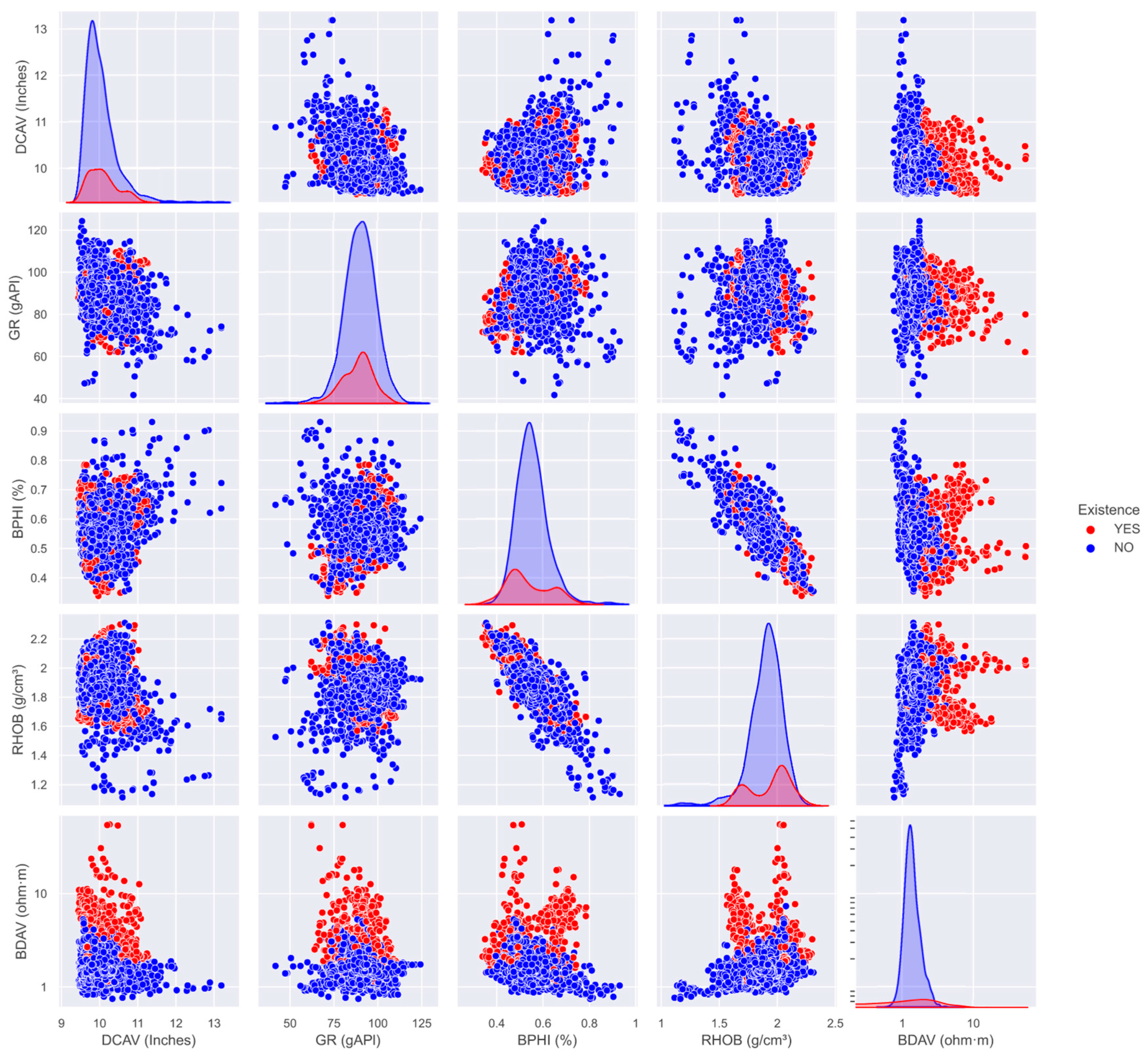
In this study, well logging data from four boreholes located within the accretionary prism of the Cascadia subduction zone will be utilized to select well logging curves that exhibit heightened sensitivity to gas hydrates. Subsequently, six ML algorithms, namely support vector machine (SVM), Gaussian process classification (GPC), multilayer perceptron (MLP), random forest (RF), extreme gradient boosting (XGBoost), and logistic regression (LR), will be employed to identify GHRs within the study area.

2. Geological Setting

The specific objective of Expedition 311 of the International Ocean Drilling Program (IODP) is to study the enrichment and formation mechanism of natural gas hydrates in aggradation complexes [36]. The study area is located in the accretionary prism of the Cascadia subduction zone. Its tectonic setting is on the accretionary wedge formed by the subduction of the Juan de Fuca plate to the North American plate, and the Juan de Fuca plate subducts downward at a speed of ~45mm/y [37,38]. Tectonic plate subduction conveys considerable sediment volumes from deep-sea basins to the outermost edge of the subduction–accretion prism, where the sediment gradually builds up. Favorable temperature and pressure conditions, coupled with an abundant supply of hydrocarbons, enable this region to host natural gas hydrates, making it a quintessential example of an active continental margin hydrate research area.

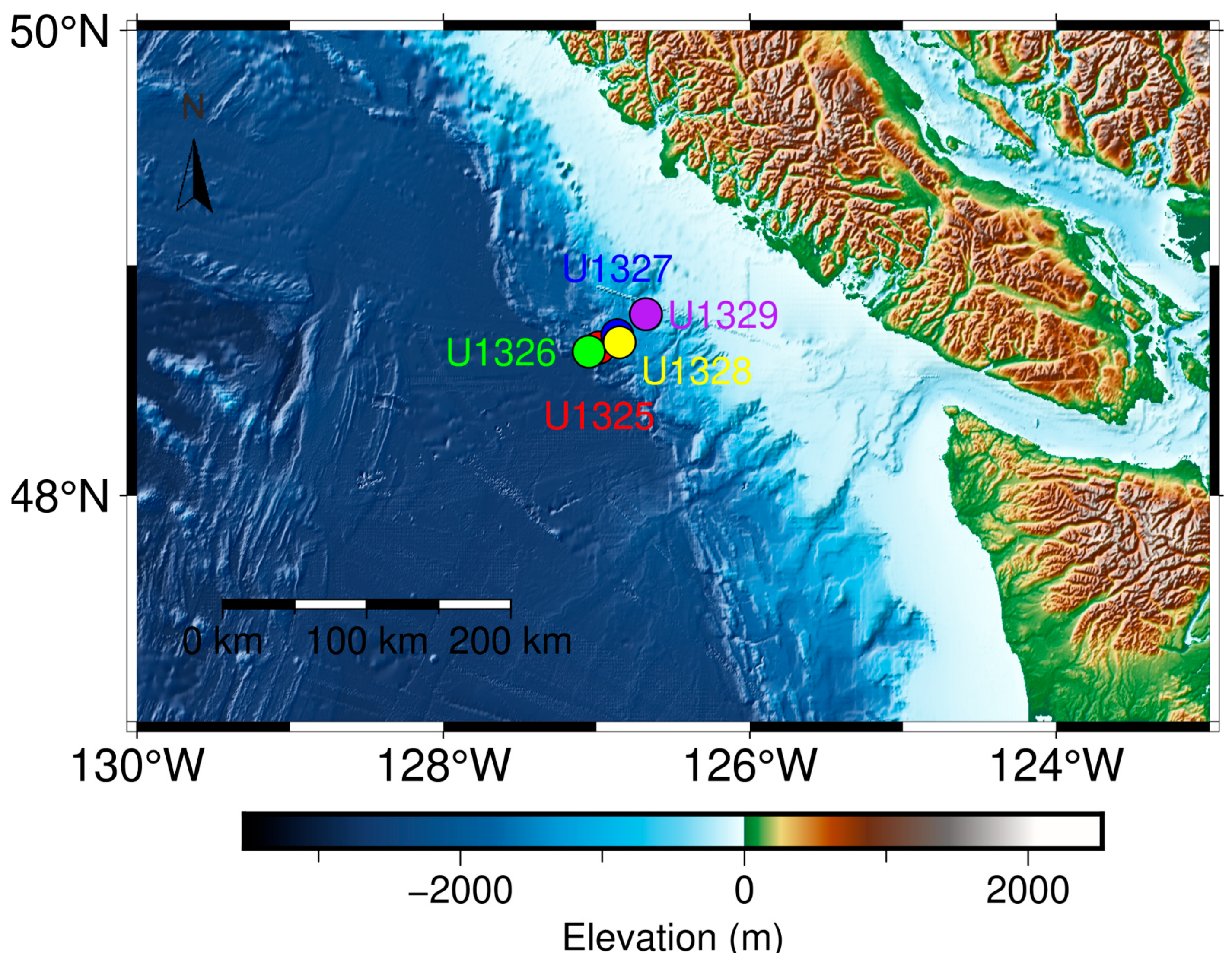
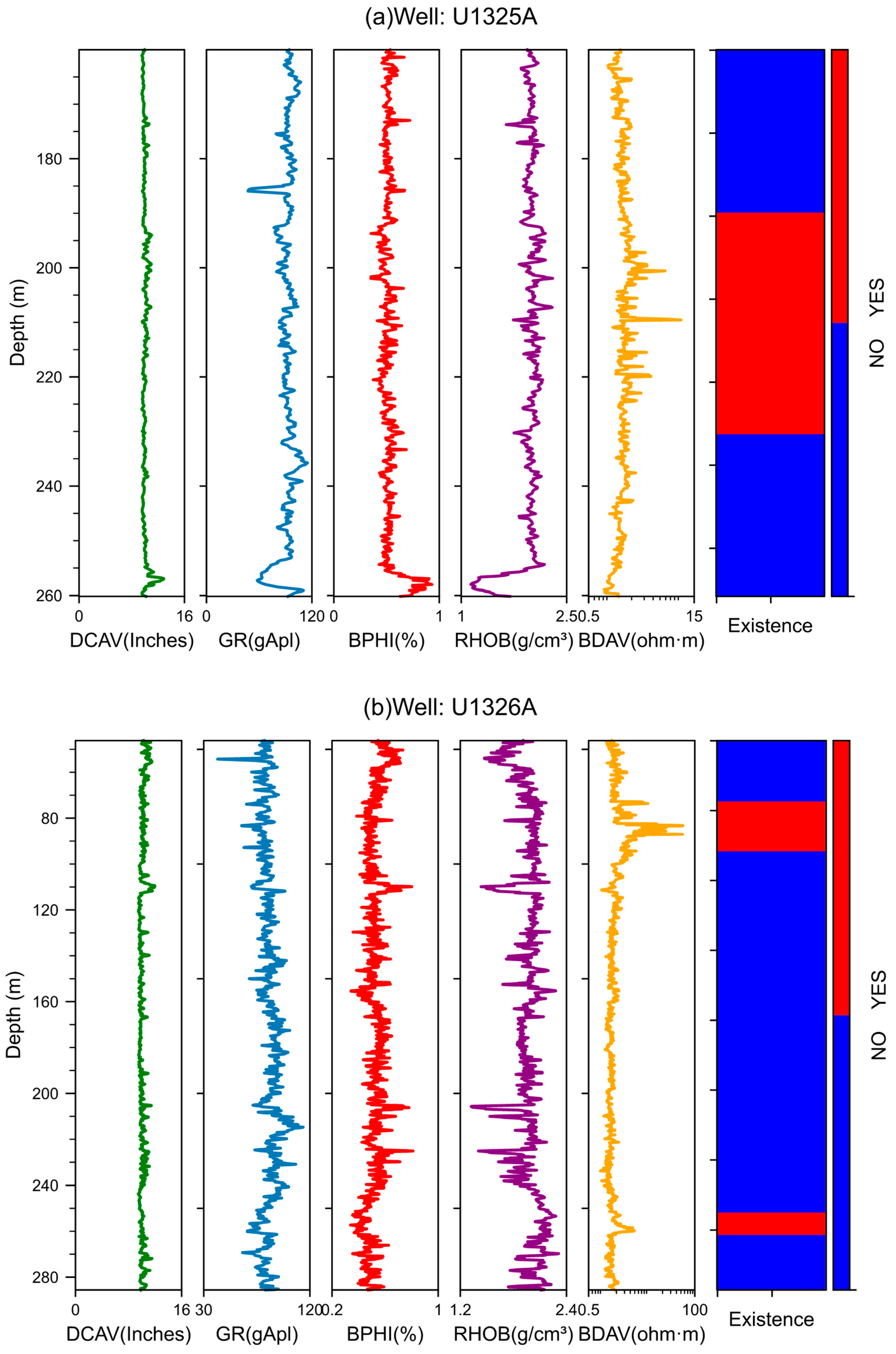
The IODP Expedition 311 was conducted from September to October 2005. Throughout the entire voyage, five stations were established at the edge of the Cascadia subduction zone, namely sites U1325, U1326, U1327, U1328, and U1329. As depicted in Figure 1, the five stations are placed in the front, middle, and back parts of the accretionary wedge, representing the different stages of gas hydrate evolution in the context of active continental margins [39]. The location information (longitude and latitude) of each borehole is shown in

Table 1. Information on the drilling locations of boreholes U1325A, U1326A, U1327A, U1328A, and U1329A during the IODP Expedition 311 [39].

Hole	Latitude	Longitude	Total Penetration
U1325A	48°38.691′ N	126°58.991′ W	350 mbsf
U1326A	48°37.635′ N	127°3.029′ W	300 mbsf
U1327A	48°41.887′ N	126°51.921′ W	300 mbsf
U1328A	48°40.072′ N	126°51.022′ W	300 mbsf
U1329A	48°47.369′ N	126°40.713′ W	220 mbsf

. Among them, the depths of U1326A, U1327A, and U1328A are 300 m below the seafloor (mbsf), while the depths of U1325A and U1329A are 350 mbsf and 220 mbsf, respectively [39].

3. Methodology

In this study, six algorithms are proposed to be used: GPC, SVM, MLP, RF, XGBoost, and LR. For model training and testing, we used logging data from boreholes in the study area and the identification of reservoir segments for gas hydrates. The underlying theoretical principles and corresponding model evaluation metrics of these algorithms are concisely summarized below.

3.1. Algorithm Introduction

3.1.1. Gaussian Classification Process

As an ML paradigm grounded in the Gaussian process, GPC is specifically formulated to tackle classification problems. The Gaussian process is a random process in which each point x corresponds to a random variable f. The joint distribution of these variables exhibits a Gaussian nature, defined via the mean and covariance functions [40]. In GPC, since the target value y of the classification problem is discrete, it is no longer assumed that y|x obeys the Gaussian distribution, but other suitable distributions, such as the Bernoulli distribution, are selected. In order to solve this problem, a latent function f (implicit variable) is introduced, and its normal prior is given. Then, the observed data (x, y) is used to calculate the potential function f and its output after passing through the response function (such as the sigmoid or probit function). These outputs are projected onto the [0, 1] range to derive the classification probability [41]. The implementation of GPC includes selecting appropriate kernel functions (such as RBF kernel, etc.) to define the covariance function of the Gaussian process, using training datasets (x, y) to train the model and obtain the posterior distribution of potential function f, and to finally predict the new input x* to obtain the classification label.

GPC performs well in dealing with nonlinear classification problems and has a strong generalization ability. However, due to its high computational complexity, approximation methods (such as Laplace approximation, expected propagation, etc.) are often used to reduce the computational complexity [42].

3.1.2. Support Vector Machine

SVM stands as a potent instrument within the domain of supervised learning, showcasing remarkable proficiency in handling both classification and regression analysis assignments [43]. The core principle involves identifying the most suitable hyperplane that maximizes the margin separating distinct categories of sample points, thereby enabling precise classification. For linear separable data, SVM constructs a decision boundary; for linear non-separable data, it is solved by mapping kernel function to high-dimensional space [44]. In addition, SVM also introduces the concept of a soft interval to allow for certain classification errors to deal with noise and outliers, and the penalty coefficient C controls the penalty intensity. SVM demonstrates robust performance in handling high-dimensional and noisy datasets, making them highly adaptable to diverse classification tasks. Additionally, SVM enables nonlinear classification via kernel-induced feature mapping, thereby extending its applicability to complex decision boundaries. Its training process involves solving convex quadratic programming problems, and its performance is highly dependent on parameter selection. It is often optimized by grid search, cross-validation, and other methods.

With regard to nonlinear functions, the SVM algorithm unfolds its general operational procedure as detailed below:

(I) First select the kernel function: K(x_i, x_j).

(II) In the feature space, we construct the following optimization problem to find the optimal separation hyperplane:

$${\min }_{\alpha }{\displaystyle \frac{1}{2}}{\displaystyle \sum _{i=1}^N{\displaystyle \sum _{j=1}^N{\alpha }_i}}{\alpha }_j{y}_i{y}_{j}K\left(x_i,x_j\right)-{\displaystyle \sum _{i=1}^N{\alpha }_i}.$$

(1)

(III) Constraints:

$$\left\{\begin{array}{c}{\displaystyle \sum _{i=1}^N}{\alpha }_i{y}_i=0\\ 0\le {\alpha }_i\le C,\hspace{1em}\forall i=1,2,\dots ,N\end{array}\right. ,$$

(2)

where α_i is the Lagrange multiplier, C is the regularization parameter, which is used to control the punishment for classification errors, and y_i is the label of the data point x_i (value ± 1).

(IV) For the purpose of resolving the above-described constrained optimization problem, the sequential minimal optimization (SMO) method, along with other convex optimization algorithms, is typically employed. After solving, we obtain the optimal Lagrange multiplier vector:

$${\alpha }^{\ast }={({\alpha }_1^{\ast },{\alpha }_2^{\ast },\dots ,{\alpha }_N^{\ast })}^T.$$

(3)

(V) Calculate the support vector in the decision function:

$$\sum _{i=1}^N{\alpha }_i^{\ast }{y}_{i}K(x,x_i).$$

(4)

(VI) Calculate the bias term and solve this equation. We can obtain a possible value of the bias term b*, which is usually calculated by using the average value of all support vectors:

$$y_s\left(\sum _{i=1}^N{\alpha }_i^{\ast }{y}_{i}K(x_s,x_i)+b^{\ast }\right)=1.$$

(5)

(VII) Finally, we build a decision function to classify the following:

$$f(x)=sign\left(\sum _{i=1}^N{a}_i^{\ast }{y}_{i}K(x,x_i)+b^{\ast }\right).$$

(6)

3.1.3. Multilayer Perceptron

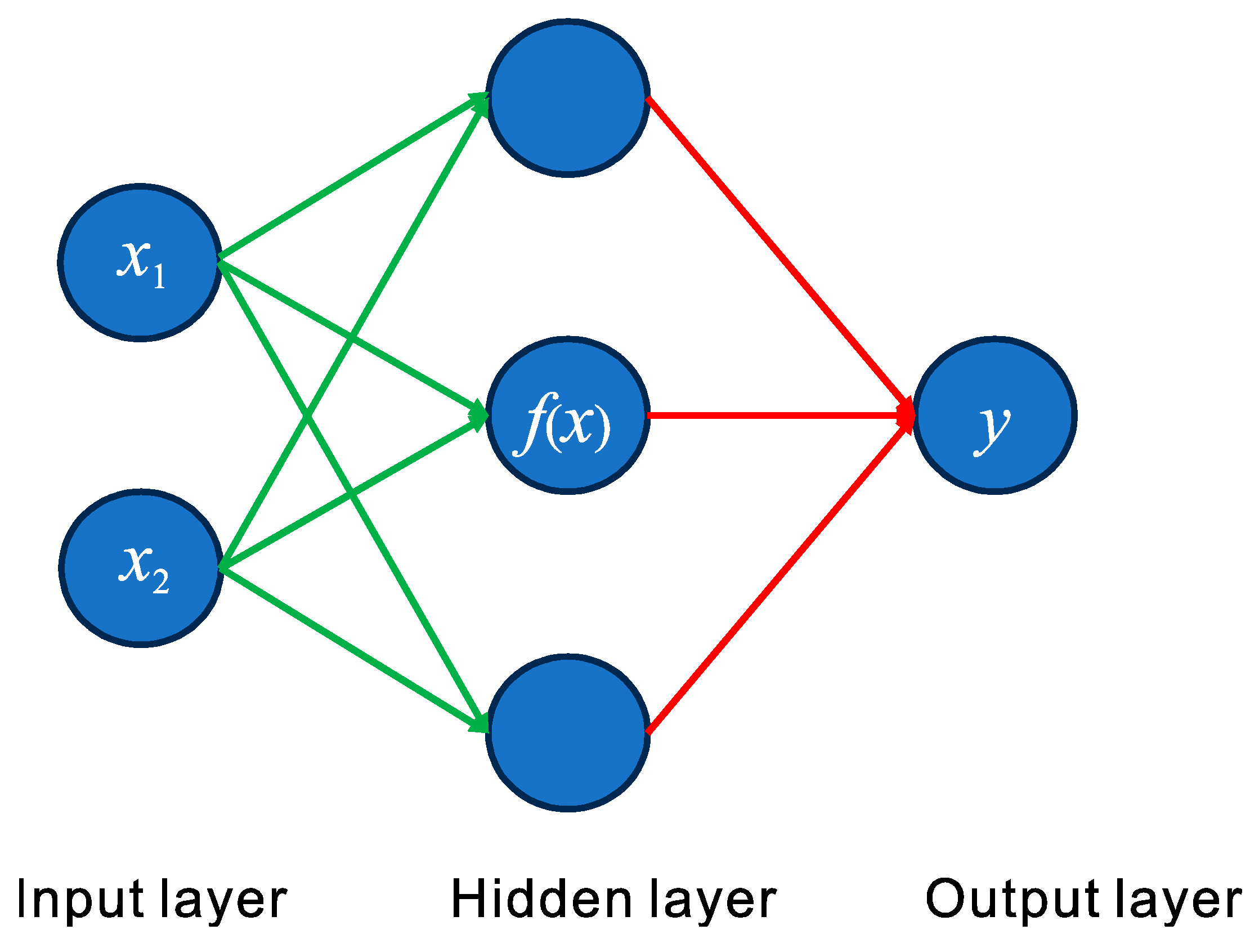
MLP serves as the foundational architecture within the realm of deep learning, encompassing an input layer, one or more hidden layers, and an output layer. The input layer assumes the responsibility of capturing raw data information. The hidden layer is dedicated to conducting feature extraction and applying nonlinear mapping to the data, and the output layer is employed to yield the final prediction results [45]. The operations of linear transformation and activation function processing are performed on the data during forward propagation. Operations are performed step-by-step through the layers, leading to the data being conveyed to the output layer [46]. The loss function is employed to gauge the discrepancy between the anticipated outcomes and the true values in the dataset. Consequently, the choice of the loss function holds significant importance. Following this, the gradient is calculated through the backpropagation mechanism, and subsequently, the model’s parameters are adjusted utilizing the gradient descent approach to attain model optimization. MLP possesses a powerful ability to represent complex relationships, making it appropriate for nonlinear issues and high-dimensional datasets. Nevertheless, it entails a substantial training time and has high requirements for data preprocessing.

Figure 2 shows the MLP with only one hidden layer, where f(x) represents the activation function, which is a nonlinear function. We determine whether neurons should be activated by calculating the weighted sum and adding bias, mainly including Sigmoid, Tanh, and ReLu.

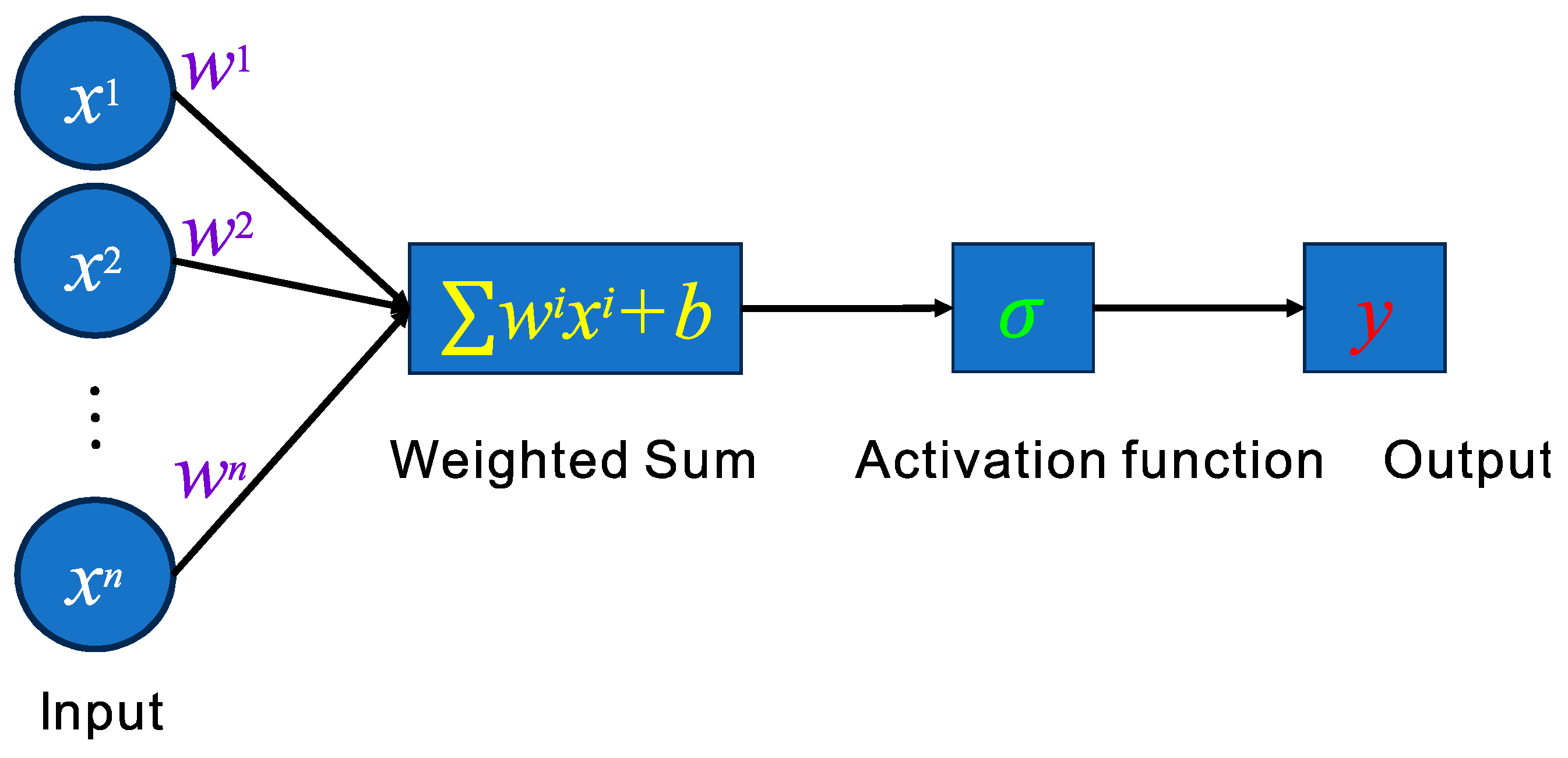
In a multilayer perceptron, every neural network layer comprises numerous neurons. The architectural details of an individual neuron are presented in Figure 3, which encompasses four components:

(I) Input: The neuron receives multiple input signals from the previous layer or external sources. These input signals are usually weighted values; that is, each input value is multiplied by a corresponding weight, and its vector expression is as follows:

$$X={[x^1,x^2,x^3,\dots ,x^n]}^T.$$

(7)

(II) Weighted summation: w₁, w₂, …, w_n is the weight of neurons, and its vector expression is as follows:

$$W=[w^1,w^2,w^3,\dots ,w^n].$$

(8)

The neuron multiplies all input signals by their corresponding weights and adds these products to obtain a weighted sum. However, in some cases, especially in neural networks, the formula of weighted summation may be extended to include a constant term b; that is, the bias term. The relevant formula is as follows:

$$z=\sum _{i=1}^n{w}^i{x}^i+b.$$

(9)

(III) Activation Function: A nonlinear activation function is employed to transform the weighted sum, thereby resulting in the output of the neuron.

(IV) Output: The outcomes derived from the processing of values by the nonlinear activation mechanism constitute the outputs produced by neurons, and its value is as follows:

$$y=\sigma (z)=\sigma (WX+b).$$

(10)

3.1.4. Logistic Regression

In the statistical learning methodology system, LR plays a crucial role and has been widely applied in various classification tasks, especially in the field of binary classification, demonstrating excellent applicability [47]. Grounded in linear models, LR employs the Sigmoid function to project input features onto a probability scale spanning from 0 to 1. This allows for a quantitative assessment of the probability that samples fall into positive classes. In particular, the Sigmoid function is employed to map the output generated by a linear model onto a probabilistic scale, and the decision function sets a threshold (such as 0.5) based on this probability value to achieve sample classification judgment. In LR, the log-likelihood loss serves to assess the deviation between the forecasted outcomes and the actual labels, thereby enabling the evaluation of prediction accuracy. When it comes to the pursuit of optimal parameters for LR, gradient descent stands as a broadly utilized optimization algorithm. It computes the gradient of the loss function relative to the parameters and iteratively modifies the parameters in the direction opposite to the gradient, thus progressively attaining the minimization of the loss function.

LR is constructed upon a linear modeling framework. Within this framework, the model’s predictions of the output are achieved through a linear combination of input features. To be more specific, linear models can be characterized by the following formula:

$$z={\beta }_0+{\beta }_1{x}_1+{\beta }_2{x}_2+\cdots +{\beta }_n{x}_n,$$

(11)

where β₀ is the intercept term, β₁, β₂, …, β_n represents the coefficient associated with the feature, and x₁, x₂, …, x_n is the input feature.

The Sigmoid function converts the output z of the linear model into the probability value p, and the formula is as follows:

$$p={\displaystyle \frac{1}{1+e^{-z}}},$$

(12)

where the probability value p represents the possibility that the sample belongs to a positive class. LR uses a decision function to convert the probability value p into a classification result. Generally, when p ≥ 0.5, the samples are classified as positive classes; when p < 0.5, the sample are classified as negative. This threshold (0.5) can be adjusted according to the actual demand.

In the LR model system, logarithmic likelihood loss is used to accurately measure the degree of difference between predicted probabilities and true labels. For the common and important application scenario of binary classification, logarithmic likelihood loss has a specific mathematical expression, and its formula is presented as follows:

$$L=-{\displaystyle \frac{1}{m}}\sum _{i=1}^m\left[y_i\log (p_i)+(1-y_i)\log (1-p_i)\right],$$

(13)

where m denotes the quantity of samples, y_i represents the actual label (either 0 or 1) of the i-th sample, and p_i signifies the predicted probability for the i-th sample.

3.1.5. Random Forest

RF is composed of multiple decision trees, which is an integrated learning method. The calculation process is a complex and delicate process, which combines the prediction results of multiple decision trees to improve the accuracy and stability of the model.

RF uses the self-help sampling method to randomly extract multiple sample book subsets D₁, D₂, …, D_n from the original training dataset D by means of put-back sampling, where n is the number of decision trees. Each sample subset D_i (i = 1, 2, …, n) contains the same number of samples as the original dataset, but the samples in D_i may be duplicated due to the put-back sampling. Each sample subset D_i is used to train a decision tree T_i independently. In the process of constructing each decision tree T_i, the RF algorithm will not use all features to split nodes. Let all available features be set to F, and the RF algorithm will randomly select a subset of features F_i ⊆ F from F. Then select the best feature to split nodes. This random feature selection method further increases the diversity of the model, which helps to reduce overfitting and improves the generalization ability of the model. When the new sample x is predicted, each decision tree T_i gives the prediction result y_i.

For the classification problem, the majority voting method is used to determine the final category y. If C is the set of category labels, the final category y can be determined by the following formula:

$$y=\arg \underset{\mathrm{c} \in C}{\max }\sum _{i=1}^{n}I\left(y_i=c\right),$$

(14)

where I (·) is the indicating function, which is 1 when y_i = c; otherwise, it is 0.

The RF algorithm has high accuracy and robustness and reduces error by integrating the prediction results of multiple decision trees. It has a strong anti-overfitting ability and uses self-help sampling method and random feature selection to increase the diversity of the models. It can process high-dimensional data and automatically select important features.

3.1.6. Extreme Gradient Boosting

XGBoost is an efficient ensemble learning algorithm that is based on the gradient lifting decision tree framework and gradually optimizes the prediction results by iteratively training multiple decision trees. Each new tree will focus on correcting the prediction error of the previous tree and finally the weighted sum of the prediction results of all trees to obtain a more accurate final prediction. In order to prevent the model from overfitting, XGBoost introduces regularization technology to control the complexity of the model. At the same time, it also supports parallel computing, which can significantly accelerate the training process. In addition, XGBoost can automatically process the missing values in the data without the need for cumbersome manual preprocessing. Because of its excellent performance and ease of use, XGBoost has been widely used in ML tasks such as classification and regression, especially for processing structured data and high-dimensional sparse data.

3.2. Performance Evaluation of Machine Learning Model

For this research endeavor, in order to obtain a comprehensive and accurate evaluation of the classification model’s performance, we adopted multiple evaluation indicators, including accuracy, precision, recall, the harmonic mean of precision and recall (F1 score), the receiver operating characteristic (ROC) curve, and the confusion matrix. These evaluation indexes play an important role in quantifying model accuracy, evaluating model robustness, and identifying model problems.

Accuracy, serving as a pivotal metric for assessing the overall efficacy of a model, holds significant importance in classification tasks. It offers a straightforward reflection of the model’s precision in forecasting sample categories, namely the proportion of samples correctly predicted by the model (including samples correctly identified as hydrate and non-hydrate) in the total samples:

$$\mathrm{Accuracy}={\displaystyle \frac{\mathrm{TP}+\mathrm{TN}}{\mathrm{TP}+\mathrm{TN}+\mathrm{FP}+\mathrm{FN}}}.$$

(15)

In the realm of model evaluation, precision signifies the fraction of samples genuinely belonging to the positive category within the set of model-predicted positive samples; that is, the proportion of samples predicted to be hydrates that are actually hydrates. Its essential significance resides in its capacity to significantly mitigate the risk of false positives in the model, subsequently enhancing the reliability of the prediction outcomes:

$$\mathrm{Precision}={\displaystyle \frac{\mathrm{TP}}{\mathrm{TP}+\mathrm{FP}}}.$$

(16)

Recall rate measures the coverage rate of positive samples; that is, the proportion correctly predicted by the model in the samples that are actually hydrate to identify more positive instances:

$$\mathrm{Recall}={\displaystyle \frac{\mathrm{TP}}{\mathrm{TP}+\mathrm{FN}}}.$$

(17)

As a holistic evaluation indicator, the F1 score ingeniously amalgamates the performance of precision and recall. It is not a simple arithmetic mean but a harmonic average calculation that takes these two factors into account. When the F1 score is high, it indicates that the model has a well-balanced and excellent performance regarding both accuracy and recall, showcasing its ability to accurately discern and fully cover classification tasks:

$$\mathrm{F}1=2\times {\displaystyle \frac{\frac{\mathrm{TP}}{\mathrm{TP}+\mathrm{FP}}\times \frac{\mathrm{TP}}{\mathrm{TP}+\mathrm{FN}}}{\frac{\mathrm{TP}}{\mathrm{TP}+\mathrm{FP}}+\frac{\mathrm{TP}}{\mathrm{TP}+\mathrm{FN}}}}={\displaystyle \frac{2\times \mathrm{TP}}{2\times \mathrm{TP}+\mathrm{FP}+\mathrm{FN}}}.$$

(18)

The true positive rate (TPR), which is also referred to as sensitivity or recall within the realm of model evaluation, is employed to ascertain the ratio of samples that a model accurately predicts as positive out of all the samples that are truly positive. It serves as a significant metric for gauging the model’s capability to recognize positive samples:

$$\mathrm{TPR}={\displaystyle \frac{\mathrm{TP}}{\mathrm{TP}+\mathrm{FN}}}=\mathrm{Recall}.$$

(19)

The false positive rate is the percentage of samples that are really negative but are wrongly predicted as positive by the model:

$$\mathrm{FPR}={\displaystyle \frac{\mathrm{FP}}{\mathrm{FP}+\mathrm{TN}}}.$$

(20)

In the field of binary classification model evaluation, the ROC curve and the area under curve (AUC) are indispensable tools. They offer an intuitive way to reflect the model’s classification performance under different threshold conditions, which is of great practical significance for optimizing model performance and making informed decisions. The ROC curve is a crucial analytical tool. This curve takes the true case rate as the vertical axis and the false positive case rate as the horizontal axis. By depicting the dynamic relationship between the two under different classification thresholds, it intuitively presents the changing trend of model performance with the adjustment of classification thresholds. This feature provides a solid theoretical foundation and analytical basis for comprehensively evaluating model performance, effectively screening key features, and reasonably evaluating model performance on imbalanced datasets. AUC, as the core quantitative indicator for measuring the classification performance of the model represented by the ROC curve, is defined as the area enclosed by the ROC curve and the coordinate axis. The range of AUC values is strictly defined between 0 and 1. When the AUC value approaches 1, it indicates that the model has a stronger ability to distinguish positive and negative samples; that is, the classification performance of the model is better. On the contrary, if the AUC value is closer to 0, it means that the classification performance of the model is worse. They are often used together to comprehensively evaluate the performance of classifiers.

The AUC, in mathematical terms, is defined as the area encompassed beneath the ROC curve. The corresponding calculation formula is as follows:

$$\mathrm{AUC}={\displaystyle {\int }_0^1(1-\mathrm{FPR}(t\left)\right)\mathrm{d}t}.$$

(21)

The confusion matrix serves as an analytical tool within the ML sphere for gauging the performance of classification models and visually representing the classification outcomes. A differentiation exists between the rows and columns within the confusion matrix. Typically, the columns of the confusion matrix correspond to predicted instances, whereas the rows denote real instances. Data points where the number of rows and columns are equal signify the count of correct predictions, while those with unequal row and column counts indicate the number of incorrect predictions. In the confusion matrix, we can not only see the overall accuracy of the prediction but also obtain the specific error point of the prediction error.

4. Results

4.1. Data

The data of this study are mainly from the logging while drilling (LWD) data of IODP Expedition 311 during the inspection using Schlumberger measurement tools. LWD tools provide conventional logging curves and special logging data. Among them, conventional logging includes Density Caliper, Average (DCAV), Gamma Ray (GR), Bulk Density (RHOB), Best Thermal Neutron Porosity, Average (BPHI), Deep Resistivity Average (BDAV), Medium resistivity, shallow resistivity, and P-wave velocity (Vp), and the sampling interval of these logging curves is 0.1524 m. Special logging includes LWD image log-Resistivity At Bit (RAB) images, and the sampling interval is 0.0305 m. As the hydrate reservoir in borehole U1329A is not clearly defined, in order not to affect the research results, the data of U1329A are not used in this study. The logging data of the other four wells and the hydrate reservoir location are shown in

Table 2. Logging data information and hydrate reservoir depth range [39,50,52,53,54].

Well ID	Logging Curves	Sampling Interval (m)	Gas Hydrate Depth Range (mbsf)
U1325A	DCAV, GR, RHOB, BPHI, BDAV, Vp	0.1524	195–230
	RAB	0.0305
U1326A	DCAV, GR, RHOB, BPHI, BDAV, Vp	0.1524	73–94, 252–261
	RAB	0.0305
U1327A	DCAV, GR, RHOB, BPHI, BDAV, Vp	0.1524	120–138
	RAB	0.0305
U1328A	DCAV, GR, RHOB, BPHI, BDAV, Vp	0.1524	20–35, 215–222
	RAB	0.0305

. According to statistics, in borehole U1325A, the interval where natural gas hydrate exists is within the depth range of 195–230 mbsf [48,49,50,51]. For borehole U1326A, scientific analysis reveals the existence of gas hydrate within the depth intervals spanning from 73 to 94 mbsf and from 252 to 261 mbsf [49,52]. In borehole U1327A, the interval containing gas hydrate is in the depth range of 120–138 mbsf [39,49,53]. In borehole U1328A, gas hydrate is distributed in the depth intervals of 20–35 mbsf and 215–222 mbsf [39,48,51,54]. We do not use sonic velocity logging data because sonic velocity logging curves are missing at some depths. Pursuant to the correlation analysis delineated in Figure 4, among the conventional logging data in the study area, five types of logging parameters, namely DCAV, GR, BPHI, RHOB, and BDAV, are chosen due to their strong correlation and high sensitivity to gas hydrate. Therefore, in this study, these five logging curves from four boreholes (U1325A, U1326A, U1327A, and U1328A) are selected as the input characteristic parameters, as shown in Figure 5.

Analysis of Log Curve Cross Plot

We selected five logging data corresponding to hydrate-bearing and hydrate-free intervals in the four boreholes and drew the transaction diagram. The results are shown in Figure 6. Among them, the blue dot represents no hydrate, and the red dot represents hydrate. It can be seen from Figure 6 that the cross plot is composed of four curves of well diameter, density, natural gamma, and porosity. The two types of data points are mixed, and the points containing hydrate and those without hydrate can hardly be distinguished. However, when the resistivity curves interact with the other four kinds of logging curves, most hydrate-bearing intervals and hydrate-free intervals are well distinguished. Nevertheless, some of the two types of data points are mixed together, which makes it difficult to distinguish quickly and accurately. To accurately differentiate between intervals containing gas hydrates and those without, this research employs a series of ML algorithms geared toward the identification of GHRs.

4.2. Data Preprocessing, Model Training, and Optimization

The data need to be preprocessed before model training. We extracted the logging data of the interval needed in this study and labeled the extracted data. Among these intervals, the one with natural gas is assigned a value of 1, while the one without is given a value of 0. Finally, a total of 3753 data were selected from the data of four wells, including 743 data containing gas hydrate and 3010 data without gas hydrate, as illustrated in Figure 7. In order to improve the fairness of the model, we use the synthetic minority oversampling technique (SMOTE) to increase the number of small samples. In the XGBoost model, we increase the minority sample to the same level as the majority sample. In the other five models, we increase the minority sample to 0.3 times the majority sample for experiments. With the aim of optimizing the model’s training efficiency and overall performance, scaling the data to a standardized range and carrying out standardization are indispensable procedures.

The standardized formula, commonly referred to as the Z-score standardization formula, serves to transform the original data into a standard normal distribution, where the mean equals 0 and the standard deviation is 1. The formula is presented below:

$$Z={\displaystyle \frac{X-\mu }{\sigma }},$$

(22)

where Z is the standardized value, and it indicates the degree to which data points deviate from the mean, X corresponds to the raw value of each individual data point, μ is the arithmetic mean of the entire dataset, and σ is the measure of dispersion, representing how much the data points deviate from the mean within the dataset.

Upon finishing data preprocessing, the dataset samples are arbitrarily split into a training set and a test set in a 3:1 ratio. We utilize the training set to support model learning, enabling the model to identify the characteristics and hidden rules within the data. In contrast, the test set is used to assess how well the trained model functions, testing its generalization capability and its accuracy. The categorization of dataset samples could potentially result in bias during model performance assessment, and cross-validation is thus adopted as a more reliable evaluation approach. This approach trains and assesses the model through the process of splitting the dataset into several subsets. Each subset is used in rotation as a validation set, while the others are employed as training sets. By adopting this approach, every subset has a chance to act as a validation set, enabling a more all-encompassing assessment of the model’s capabilities across various data subsets. In the pursuit of model performance optimization, hyperparameter optimization is an indispensable link [55]. Grid search functions as a method for optimizing hyperparameters. It can systematically traverse the combination of multiple parameters and determine the best effect parameters through cross-validation. Its general principle is to first specify a value range for each hyperparameter. Then, the grid search algorithm will traverse all the combinations in the grid and use cross-validation for each group of parameters to evaluate the effect. Finally, the grid search will output the best combination of parameters based on the results of cross-validation; that is, those parameters that perform best in all cross-validation rounds. For this investigation, the grid search strategy is employed to optimize the hyperparameters of the four classifiers, and the 5-fold cross-validation approach is adopted to assess the model’s performance across every parameter configuration. This strategy not only enhances the efficiency while elevating the accuracy of model optimization but also offers us a more comprehensive and robust model evaluation framework, laying a solid foundation for subsequent research and application.

4.3. Identification Results

In this study, we use six different models to identify marine GHRs. The results of each model are obtained from the fine-tuning optimal model using the grid search method. The best parameter selection is shown in

Table 3. Optimal hyperparameter selection of six models.

Model	Hyperparameter (Symbol)	Parameter Value
GPC	Default setting	Default setting
SVM	Kernel	RBF
	Penalty coefficient (c)	10
	Gamma	1
MLP	Regularization parameters (alpha)	0.0001
	Maximum number of iterations (max iter)	100
	Initialization learning rate (learning rate init)	0.01
	Optimization algorithms (solver)	Adam
	Batch size (batch size)	100
	Hidden layer configuration (hidden layer sizes)	100
RF	Random selection of features (max features)	3
	Minimum sample size for node splitting (min samples split)	6
	The maximum depth of a tree (max depth)	15
	The number of trees (n estimators)	30
XGBoost	Learning rate	0.1
	The number of trees (n estimators)	200
	The maximum depth of a tree (max depth)	7
	Minimum sample size for node splitting (min child weight)	1
	Gamma	0.1
	Subsample	0.6
	Colsample bytree	0.8
LR	Default setting	Default setting

.

Table 4. Accuracy, precision, recall, and F1 score of six models.

Model Type	Accuracy	Precision	Recall	F1 Score
SVM	0.9105	0.9062	0.9105	0.9070
GPC	0.8988	0.8925	0.8988	0.8926
MLP	0.9095	0.9052	0.9095	0.9060
RF	0.9191	0.9154	0.9191	0.9153
XGBoost	0.8860	0.6340	0.7736	0.6969
LR	0.8871	0.8791	0.8871	0.8746

presents the numerical values of the determined evaluation indicators. Figure 8 displays the ROC curves along with the corresponding AUC values for the six models.

4.3.1. GPC Identification Results

We use logging data as input characteristics to construct a Gaussian process to simulate the potential distribution of data based on the GPC algorithm and then classify and predict GHRs. During the construction of the GPC and recognition model, the kernel sets the initial values of a set of hyperparameters to start the first optimization process. In the subsequent iterative optimization, the value of the hyperparameter will be randomly selected from the preset reasonable value range. As shown in Table 3, the default parameter values of the Gaussian classification algorithm in scikit learn are used in this study.

Within the test set, the GPC recognition accuracy stands at 0.8988, fully attesting to its effectiveness in recognizing natural gas hydrates. The excellent performance of GPC with respect to this index indicates its capability to precisely detect the presence of natural gas hydrate based on logging data. In terms of precision, GPC also performed well, reaching 0.8925. In the task of natural gas hydrate identification, positive samples usually refer to the logging data containing natural gas hydrate. The high performance of GPC in terms of precision shows that it can effectively identify these positive samples, thus reducing the possibility of misjudgment. At the same time, its recall rate is as high as 0.8988, which means that the algorithm can identify the vast majority of actual positive samples in the test set. This result further verifies the stability and reliability of the GPC algorithm in the natural gas hydrate recognition task. The F1 score of the algorithm is 0.8926, which is between the accuracy and recall metrics. This shows that the algorithm can balance these two indicators well. In addition, the AUC value (0.9022), a key metric for evaluating the model’s classification capability, also underscores the GPC model’s excellent performance in differentiating gas hydrate and non-hydrate samples. Therefore, it can be inferred that the algorithm performs well in the task of natural gas hydrate recognition.

4.3.2. SVM Identification Results

SVM separates different types of samples by constructing the optimal hyperplane. SVM achieves high-precision classification prediction on logging data. During the construction of an SVM model, the choice of parameters substantially influences the model’s performance. To precisely ascertain the optimal parameters, this research employed the grid search approach integrated with 5-fold cross-validation. Finally, the parameter value that shows the best classification accuracy on the test set is determined as c = 10, γ = 1, and the kernel function is RBF type.

Following the optimization of model parameters and their deployment on the testing dataset, a set of crucial evaluation metrics is acquired. In the evaluation, the model yields an accuracy of 0.9105, a precision of 0.9062, a recall rate of 0.9105, and an F1 score of 0.9070. Concurrently, the area under the ROC curve of the model registers at 0.8973, with the ROC curve depicted in Figure 8. In light of the preceding metrics, we ascertain that the SVM model demonstrates robust performance in discerning natural gas hydrate, boasting high accuracy, precision, recall rate, and F1 score. At the same time, the AUC value additionally indicates that the model exhibits competent classification capabilities. This implies that the model exhibits high reliability and practicability in practical application, thereby offering robust assistance in the detection and identification of natural gas hydrate.

4.3.3. MLP Identification Results

MLP learns the nonlinear characteristics of data by constructing multiple hidden layers, and the MLP model achieves high-precision classification and prediction on logging data. In this model, we optimize the regularization parameters, maximum number of iterations, initialization learning rate, optimization algorithm, batch size, and hidden layer size. As indicated in Table 3, via the grid search approach, the regularization parameter is configured at 0.0001, while the model’s maximum iteration count is 100 and the initial learning rate is set to 0.01. Opt for the ‘Adam’ optimization algorithm, with each training iteration utilizing 100 samples, and set the number of neurons in the hidden layer to 100. Upon deploying the meticulously tuned model on the test dataset, a comprehensive set of evaluation metrics pertaining to the model’s performance is derived. The accuracy, precision, recall rate, and F1 score are 0.9095, 0.9052, 0.9095, and 0.9060, respectively. The AUC value of this model reaches 0.9180, and the ROC curve is shown in Figure 8. According to the comprehensive analysis of the above evaluation indexes, the MLP model shows excellent classification performance in the identification of natural gas hydrate. It has high-precision prediction ability, stable evaluation index, strong feature learning ability, and performs well in dealing with complex nonlinear relationships and data feature extraction.

4.3.4. LR Identification Results

As a classical linear classification algorithm, LR has also been applied to the task of gas hydrate recognition. Although its performance may not be as good as that of nonlinear models (such as GPC, SVM, and MLP), the LR model can still play a certain role in some specific cases. Following the implementation of grid search coupled with cross-validation, the parameters adopted by LR are determined to be the default parameters in the scikit learn library. After being applied to the test data, the evaluation index of the model is obtained. The model achieved an accuracy of 0.8871, a precision of 0.8791, a recall rate of 0.8871, and an F1 score of 0.8746. Additionally, the AUC metric for the model was recorded as 0.8723, with the corresponding ROC curve depicted in Figure 8.

Among the six models, the reason for the poor performance of LR may be that the algorithm has some limitations in dealing with nonlinear features, which may affect its performance in the task of natural gas hydrate recognition. It also indicates that the model exhibits relatively poor performance in differentiating between gas hydrate specimens and their non-hydrate counterparts. In summary, the LR model shows good performance in the task of gas hydrate recognition. In some specific cases, such as linear separable data, the LR model is still a choice worth considering.

4.3.5. RF Identification Results

RF builds a strong classification model by integrating multiple decision trees and using a bagging strategy. The RF model shows excellent classification performance in the task of gas hydrate recognition. In order to determine the optimal parameters, the grid search method and 5-fold cross-validation are used to find the optimal parameter combination in the process of establishing the RF model. As shown in Table 3, we set the random selection of features to 3, the minimum sample size for node splitting to 6, the maximum depth of the tree to 15, and the number of trees to 30. Finally, we apply the set parameters to the model and obtain a series of evaluation indexes of the model. The accuracy, precision, recall rate, and F1 score were 0.9191, 0.9154, 0.9191, and 0.9153, respectively, and the AUC value of the model reached 0.9314. The ROC curve is shown in Figure 7. Based on the above indicators, it can be clearly concluded that among the six comparison models, the indicators of the RF model rank first, especially in the identification of natural gas hydrate. The RF model has high accuracy, precision, recall rate, F1 score, and AUC value. This means that the RF model, with its excellent classification performance and generalization ability, shows significant application value in the actual detection scenario of natural gas hydrate and provides strong technical support for the efficient identification of potential reservoirs and optimization of exploration decisions.

4.3.6. XGBoost Identification Results

XGBoost, as an integrated learning algorithm based on a gradient lifting decision tree, shows certain feature learning ability in natural gas hydrate recognition task by iteratively optimizing residuals and introducing regularization items to prevent overfitting. Parameter settings are shown in Figure 3. However, according to the evaluation results of the current model, its comprehensive performance does not meet the expected application standards. In the test set, the accuracy, precision, recall rate, F1 score, and AUC value are 0.8860, 0.6340, 0.7736, 0.6969, and 0.9243, respectively.

Although the AUC value (0.9243) indicates that the model has a certain classification ability, the following key indicators reveal its limitations: (1) The accuracy is insufficient. The precision (0.6340) is significantly lower than that of similar models (such as 0.9108 of SVM), indicating that the actual positive samples accounted for only 63.4% of the samples predicted as “natural gas hydrate” by the model, and the risk of false positives is high, which may increase the exploration cost. (2) The F1 score is low. The F1 value (0.6969) comprehensively reflects the balance between accuracy and recall. The index below 0.7 indicates that the model has obvious shortcomings in distinguishing positive and negative samples, which cannot meet the needs of high-precision detection.

Comprehensive evaluation conclusion: The current XGBoost model performs poorly in the task of natural gas hydrate recognition, and its lack of precision, low F1 score, and low feature overlap may lead to a high misjudgment rate in practical application. Combined with the excellent performance of SVM and other comparative models, we recommend carefully evaluating the applicability of XGBoost in this scenario and giving priority to other algorithms or further optimizing the performance through feature engineering.

4.4. SHapley Additive exPlanations Value Analysis of Six Models

SHapley Additive exPlanations (SHAP) analysis reveals differences in feature contribution patterns and model behavior of different ML models in natural gas hydrate recognition tasks. The SHAP summary diagram of the six models of SVM, RF, LR, GPC, MLP, and XGBoost is shown in Figure 9.

As shown in Figure 9, RHOB and BDAV are key features for identifying natural gas hydrates in the SVM model, which have significant impacts on the model output and have diverse directions of influence. The RF model shows that BDAV and RHOB are much more important than other features, and these two features may have a positive or negative impact on the model output in different situations. In the LR model, BDAV dominates and mainly exhibits a positive impact, while GR mainly exhibits a negative impact, reflecting the linear regression model’s ability to capture the linear relationship between features and target variables. In the GPC model, BDAV and RHOB are equally important, and all features have diverse directions of influence, demonstrating the flexibility of GPC models in handling complex nonlinear relationships. In the MLP model, the importance of BDAV and RHOB is prominent, and their influence directions are diverse, which reflects the strong capturing ability of the multilayer perceptron model as a neural network model for nonlinear relationships. Finally, in the XGBoost model, BDAV is a key predictive factor, mainly manifested as a positive impact, indicating that the XGBoost model highly relies on BDAV features when identifying natural gas hydrates.

In summary, through a simple analysis of the SHAP summary graphs of six models, we have revealed the key features, feature influence directions, and differences between models in the task of identifying natural gas hydrates for each model. These pieces of information provide an important basis for understanding model behavior, optimizing model performance, and selecting more suitable models for natural gas hydrate identification.

5. Discussion

In this study, six ML algorithms are applied to train the logging data from four wells of the IODP Expedition 311. Through data preprocessing and hyperparameter optimization of the model, the samples with and without gas hydrate layers are identified. A range of evaluation metrics, encompassing accuracy, precision, recall, the F1 score, the AUC value, and the ROC curve, are leveraged to assess the efficacy of distinct ML models in hydrate recognition tasks. Next, model performance, parameter optimization, model comparison, and research limitations will be discussed in depth based on the experimental results.

5.1. Comparison of Six Machine Learning Methods

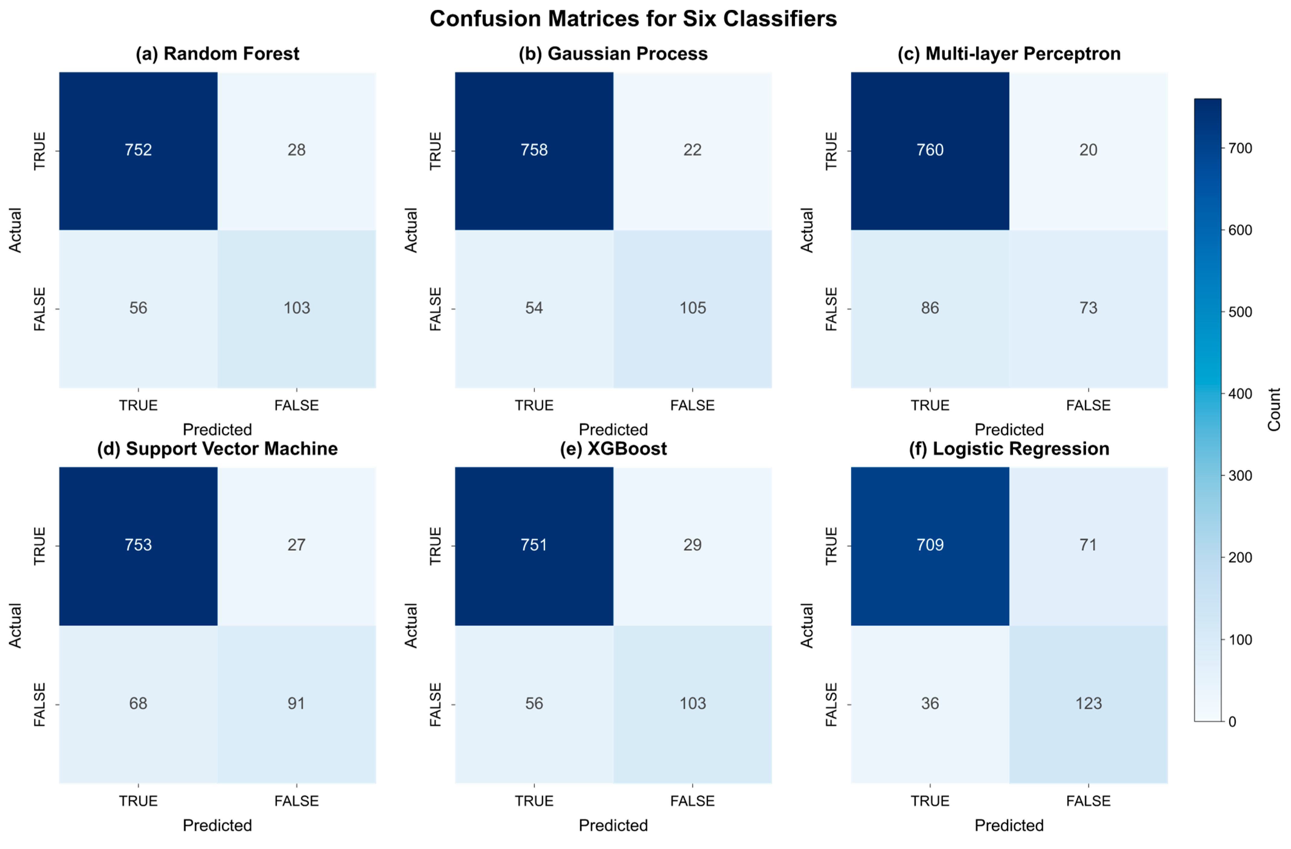
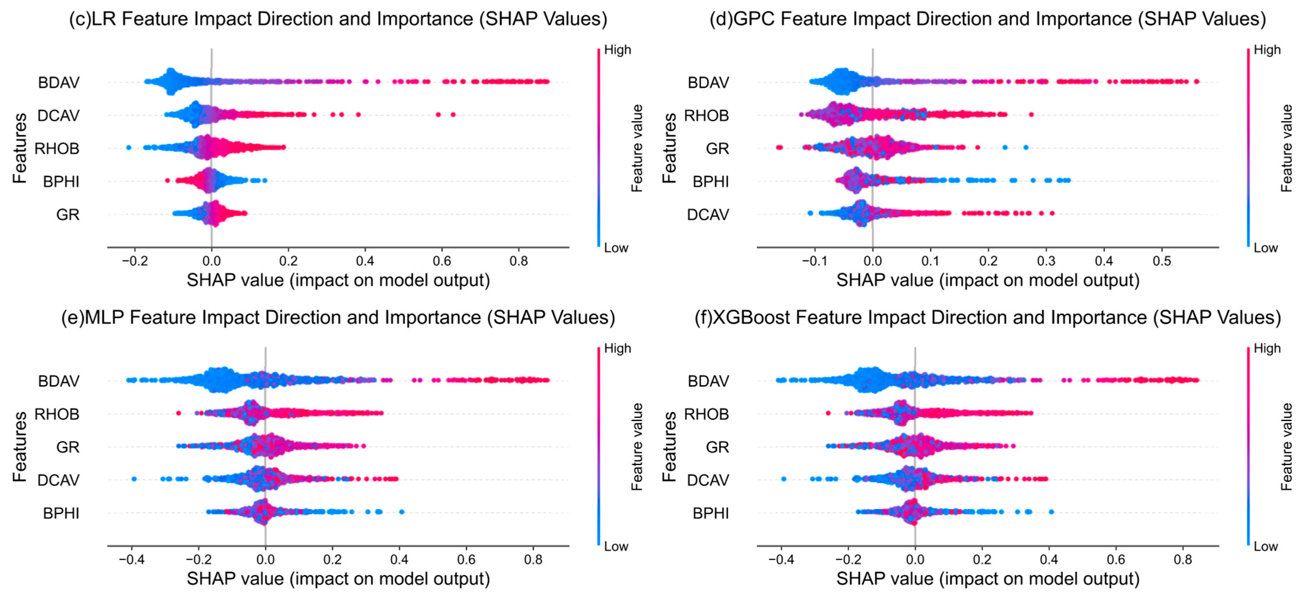
This study demonstrates the various evaluation metrics (Table 4), ROC curves and AUC values (Figure 8), and the prediction confusion matrices (Figure 10) of each model for hydrate identification by the six ML methods. From the synthesis of these indicators, the six ML models have shown certain accuracy in the task of GHR identification. Among them, the indicators of SVM, MLP, and RF have reached more than 0.90, and the RF indicators are the highest, which is the best performance of the six models. This shows that for this binary classification problem, the RF model constructs a strong classification model by integrating multiple decision trees and using the Bagging strategy and realizes the optimal distinction between GHRs and non-reservoirs. Its accuracy, precision, recall rate, F1 score, and AUC value rank first among the six comparison models, thus achieving the effect of accurately and efficiently identifying GHRs. For the high score indicators presented by MLP and SVM, it also shows that the MLP model, as a kind of deep learning, can learn the complex mapping relationship between logging data and hydrate reservoir characteristics through the training of a multilayer neural network and can also play a good role in recognition. The SVM model can effectively distinguish GHRs from non-reservoirs by finding the optimal hyperplane, so as to achieve the effect of accurately identifying GHRs. For GPC and LR models, the evaluation indexes are close to 0.90, although they are not reached, and the overall recognition effect is good. The reason why the GPC effect is slightly inferior to the first two may be related to parameter settings or data characteristics. The reason why the LR effect is slightly inferior may be that the LR model, as a linear classifier, is relatively weak in nonlinear problems, which has a certain impact on its ability to identify GHRs under complex geological conditions. For XGBoost, its overall performance is relatively weak compared with the other five models, which may be due to the model’s insufficient ability to capture complex nonlinear relationships in logging data or its limited ability to distinguish GHR boundary characteristics.

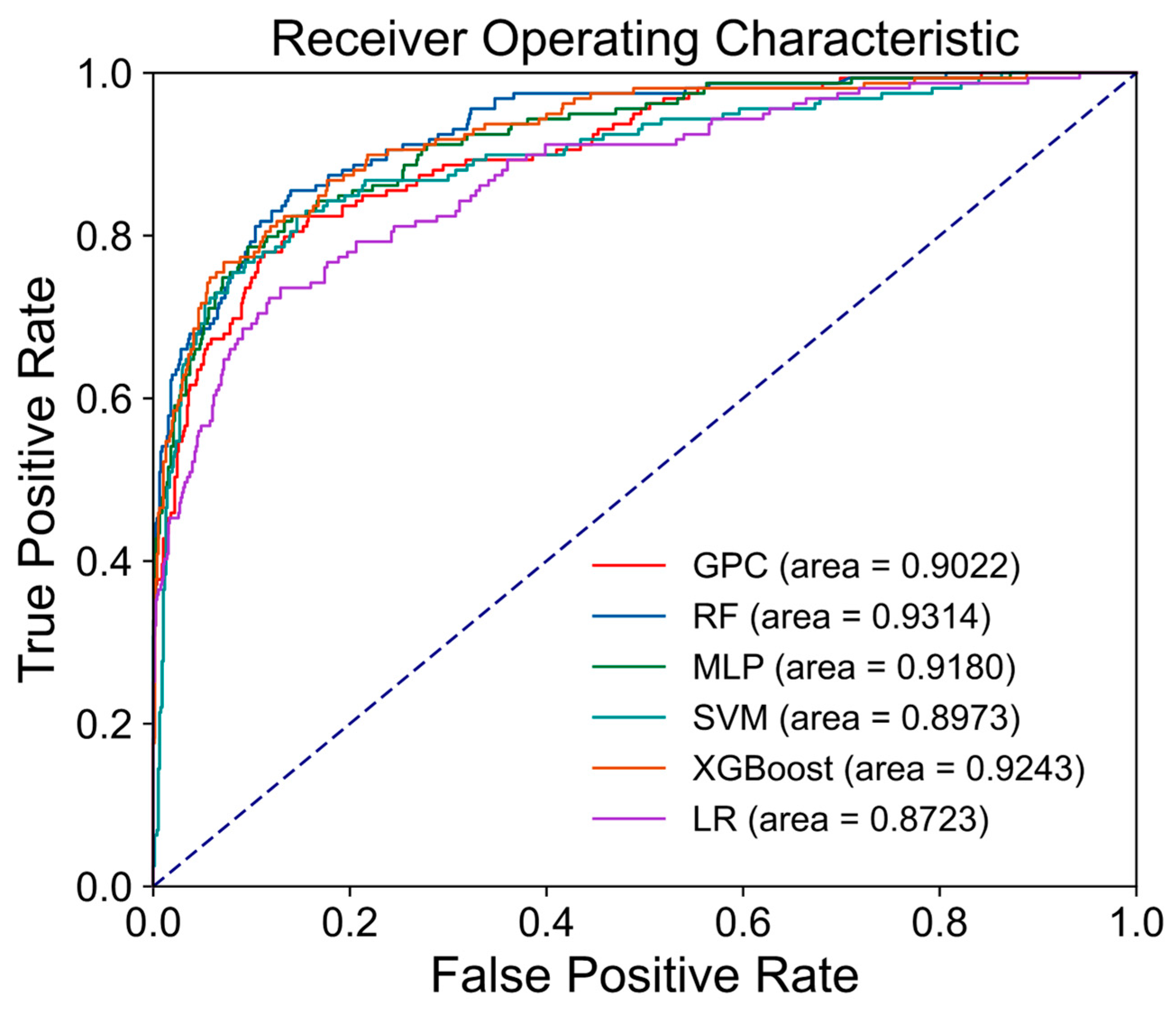
The AUC value is a key indicator for evaluating classifier performance. As presented in Figure 8, the AUC values of the six models are ordered as follows: RF > XGBoost > MLP > GPC > SVM > LR. Among them, the AUC value of RF is the highest, reaching 0.9314, and GPC is slightly lower than MLP, which is 0.9022. Although the AUC value of MLP is slightly higher than that of GPC, considering that the calculation of the AUC value has certain randomness and volatility, the difference between them is not significant. It can be considered that the performance of MLP and GPC models is equivalent. The AUC value of SVM is 0.8973, which is not as high as the first two, but still at a high level, which indicates that the model has a certain application value in the task of GHR identification. The AUC value of LR is 0.8723, which has reached an acceptable level, but there is still a certain gap compared with other models. Although other indicators of XGBoost are low, its AUC value is 0.9243. The high AUC of XGBoost indicates that it has the overall classification potential to be developed.

According to the analysis of various indicators, although the XGBoost model performs well in terms of its AUC value, its accuracy and F1 score are significantly lower than other models. Through further analysis of model characteristics and data characteristics, we found that the reason may be the mismatch between model complexity and data support. Although the class distribution is balanced through smote, the limited amount of data (especially labeled samples) is still not enough to support XGBoost to fully learn complex nonlinear patterns. Unlike the linear constraint of the LR model, the main challenge of XGBoost is to avoid overfitting and optimize the interactive expression of features.

5.2. Advantages and Limitations of Machine Learning Methods

The traditional method of identifying GHRs using logging data is usually based on an empirical formula and the intersection diagram method. However, the recognition effect of these methods usually depends on the experience of logging interpretation personnel, and the recognition efficiency is low. It commonly poses a challenge to precisely define the nonlinear relationship between logging data and GHRs. This study is based on a data-driven method, using different ML algorithms to train the relationship between the input parameters (logging data) and the output results (whether there is a hydrate layer or not). Except for XGBboost, which needs to be used with caution, the accuracy of the other five models is higher than 0.88. The recognition effect is good, and the discrimination classification model constructed by them is not interfered with by logging interpretation personnel, with high efficiency.

This study leverages an extensive collection of well logging data along with labeled hydrate reservoir data to form the training samples. Given the paucity of samples, the model’s training performance could be profoundly impacted, thereby leading to a reduction in its generalization capacity and prediction accuracy. Furthermore, due to the fact that the number of hydrate-bearing reservoirs is less than that of non-hydrate-bearing reservoirs in actual boreholes, the number of samples in these two categories is unbalanced, which may have a certain impact on the accuracy of ML.

5.3. Model Limitations and Transferability Across Geological Settings

The study area of this paper is located in the accretionary prism area of the Cascadia subduction zone. The geological conditions of the region (such as marine sedimentary environment and specific tectonic background) may limit the universality of the model. The limitations of the model are as follows: (1) The correlation between the response characteristics of logging curves and geological parameters may vary due to differences in sedimentary facies or lithological combinations. For example, in areas with active tectonic activity or permafrost on land, there are significant differences in the occurrence state of hydrates compared to the marine environment, leading to a decrease in the predictive ability of model input parameters. (2) Although ML models can capture nonlinear relationships, they may overlook the physical mechanisms of geological processes, leading to prediction biases in extreme geological conditions. (3) The weight or feature combination of logging curves may be optimal in the IODP Expedition 311 region, but the key parameters in other regions may be different. Consequently, the algorithm of the model developed in this research is predominantly suitable for regions with similar formation lithology as the study area. When dealing with regions that have considerable lithological differences relative to the study area, retraining the model and adjusting its parameters become necessary.

5.4. Ideas for Further Investigations

This study relies on the available logging data, whose quality and volume might impose constraints. As a recommendation for future studies, the multi-source data of geology, geophysics, geochemistry, and other disciplines can be combined to conduct a more comprehensive study on the reservoir identification method of natural gas hydrate. Moreover, the ML approach utilized in this research can be integrated with other cutting-edge techniques, including, but not limited to, deep learning and ensemble learning, to enhance the model’s recognition precision and generalization capacity.

6. Conclusions

In this study, the logging information from four boreholes related to natural gas hydrates within the research zone is integrated into the training samples as feature inputs, and whether the formation contains gas hydrates is used as a label. Six ML algorithms are used to identify GHRs. The evaluation of the classification model’s performance is carried out by a range of performance indicators, encompassing accuracy, precision, recall, the F1 score, the ROC, and the AUC. The following conclusions can be drawn:

(1) Except for the XGBoost model, the accuracy of the other five models is higher than 0.89, which shows that these models can effectively identify GHRs. The evaluation scores of these models are RF, SVM, MLP, GPC, LR, and XGBoost in descending order.

(2) Compared with the traditional intersection diagram method to identify GHRs, the ML method can independently establish a model to characterize the nonlinear relationship between logging data and GHRs through a data-driven method. The discriminant classification model constructed by the ML method can effectively reduce the impact of human intervention in the process of logging interpretation and significantly improve the efficiency of interpretation. Consequently, it introduces an innovative concept and approach for the identification of GHRs, which establishes a basis for the subsequent prospecting and exploitation of natural gas hydrate resources.