Abstract
Power output and economic cost are two critical factors influencing the layout of tidal stream turbine arrays. To identify the optimal configuration, this study establishes a two-objective optimization framework that simultaneously considers these factors. Both the spatial location and yaw angle of each turbine are optimized to enhance overall power output, while the total length of submarine cables, which is used to transmit electricity from the turbines to the onshore power station, is adopted as the metric for economic cost. The Huludao water area is selected as the study domain. A 12-turbine array is examined under varying weight coefficients to investigate the trade-off between maximizing power output and minimizing economic cost. The optimization results show that submarine cable length decreases linearly as its economic weight coefficient increases, while the array’s power output exhibits a stepwise decline. This indicates that, with carefully chosen weight coefficients, economic costs can be significantly reduced without a proportional sacrifice in power output. Furthermore, increasing the number of turbines connected by a single cable not only enhances power output but also reduces total cable length, thereby improving the overall profitability of the optimized array layout.
1. Introduction
The increasingly pressing environmental challenges and the growing human demand for energy highlight the urgent need to develop clean, renewable energy sources [1]. In particular, the extensive reliance on fossil fuel, which currently dominates energy consumption, leads to many environmental problems like global warming and rising sea levels [2]. Therefore, the development of renewable energy sources is essential for the sustainable growth of human society. As one of the clean and renewable ocean energy resources, tidal stream energy utilization has been widely studied.
Tidal stream turbines serve as the primary devices to convert tidal energy into electrical power. Efforts have been devoted to improving the energy efficiency of these devices. For example, Li et al. [3] optimized the shape of turbine blades using genetic algorithms and artificial neural networks, resulting in an 8.5% improvement in the maximum power coefficient. Zhu [4] adjusted the pitch angle and chord length of the blades using neural networks, achieving a 2% increase in the power coefficient and also expanding the optimal tip speed ratio range. Despite these advancements, the power output of a single turbine remains constrained. The commercialization of tidal stream energy technology will likely hinge on the deployment of large-scale arrays, which might comprise dozens or even hundreds of turbines.
However, the total power output of a tidal stream turbine array may be compromised by an increasing number of turbines if the turbine interactions are neglected [5]. The wake effect from upstream turbines reduces the power output of the downstream turbines due to reduced flow velocity [6]. To maximize the energy extracted by turbine arrays, turbines within the array should be carefully placed. In fact, optimizing the array layout can leverage the blocking effect and minimize the negative interactions caused by turbine wakes, thereby enhancing the overall performance [7]. Numerous optimization methods have been developed for the location optimization of turbines within the array. Among them, OpenTidalFarm, an open-source solver based on PDE-constrained gradient optimization, has been proved a promising tool to optimize the layout of tidal turbines [8]. Gauvin-Tremblay et al. [7] simulated an idealized shallow water channel with stable unidirectional flow using OpenTidalFarm, introducing the concept of a globally quasi-optimal solution to optimize turbine layouts, resulting in an increase in power output up to 50%.
Additionally, the yaw angle is a critical factor that significantly influences the performance of the tidal array. The tidal stream turbine is subjected to the yawed condition when the turbine axis does not align with the flow direction. The yaw angle leads to the wake deflection of the turbine, which possibly improves the power performance of the downstream turbines [9,10]. In the wind energy industry, tuning yaw angles of turbines has been found effective in improving the overall performance of the wind turbine array. For example, Lin et al. [11] and Dou et al. [12] successfully employed an active yaw control strategy to improve the maximum power output of wind turbine arrays. Since the tidal stream turbines share similarities with wind turbines [13], adjusting the yaw angle of each tidal stream turbine within the array could also be of great significance to enhance the array’s overall performance. However, the active yaw control has not been directly considered in the design of the tidal stream turbine array layout.
Regarding tidal stream energy projects, economic cost is another essential factor that should be considered. Lower construction costs can translate into shorter payback periods and increased investment appeal for stakeholders [14]. Similar to power output, construction costs are influenced by the micro-layout of the tidal stream turbine array [15]. For example, a significant cost factor influenced by the specific arrangement of the turbines is the length of submarine cables, which connect all turbines to the onshore power station to ensure electricity transmission [16,17,18]. Segura et al. [19] considered submarine cable length as an important cost in the development of tidal stream energy projects. As highlighted in the research by Vazquez and Iglesias [20], approximately 13% of the total investment expenditures are related to the cost of submarine cables.
Currently, some studies have incorporated economic costs into the optimization of turbine arrays [15,21]. However, these studies typically focus only on optimizing the spatial locations of turbines to improve array power output, while neglecting yaw effects, even though yawed flow conditions are common in real-world marine environments. Additionally, although the cost of submarine cables constitutes a substantial portion of the total expenditure for tidal stream turbine arrays, this factor has received limited attention in existing research. Few studies have considered variations in cable capacity, defined as the maximum number of turbines that can be connected by a single cable, or examined how this constraint influences turbine grouping, connection order, and the overall array layout.
Therefore, this study proposes an optimization framework that considers both the power output and economic cost of the turbine array. Specifically, the location and yaw angle of each turbine are treated as adjustable factors in the optimization process. The submarine cable length is used as an indicator of economic cost, and the variation in cable capacity is considered. The waterway between Putuoshan Island and Hulu Island is selected as the study area to demonstrate the progressiveness of this optimization framework. The characteristics of optimal results with varying weight coefficient values for the two optimization objectives are compared. Furthermore, the impact of cable capacity, which determines the maximum number of turbines that can be connected by a single cable, on the optimization results is also examined.
2. Materials and Methods
2.1. Hydrodynamic Model
The mathematical model employed in this study is based on Thetis [19], an open-source ocean numerical modeling framework. Given that the length and width scales of the simulated sea area are usually significantly larger than the water depth, the two-dimensional hydrodynamic model of Thetis is employed, which allows for an efficient simulation of tidal stream dynamics within the simulation domain.
where represents the free surface elevation, is time, is the average water depth, is the depth-averaged velocity vector, is the kinematic viscosity coefficient, and ∇ is the gradient operator ; is the Coriolis force frequency, where , , ω is the angular frequency of the Earth’s rotation, is the latitude of the simulation area, usually selected as the average latitude of the simulation area, is the latitudinal coordinate; can be obtained by rotating the two-dimensional velocity vector counterclockwise by 90°; is the bottom shear force of the simulated area, which can be calculated using the following formula [22]:
where is the acceleration due to gravity, is the Manning coefficient, mainly determined by the particle size of seabed sediment. is the dimensionless thrust coefficient of the turbine.
2.2. Presentation of Yawed Tidal Stream Turbines
In this study, we take the horizontal-axis tidal stream turbines into consideration. Defining the thrust coefficient of the turbine as , the thrust force of a yawed turbine can be expressed as:
where is the inflow velocity, is the area of the turbine’s rotation plane, is the yaw angle.
However, in the numerical model, it is more important to obtain the flow velocity through the turbine resistance distribution area, , when calculating the thrust force. For instance, in Thetis, the thrust force of the turbine is expressed as:
where is the turbine resistance distribution area, is the dimensionless thrust coefficient of the turbine.
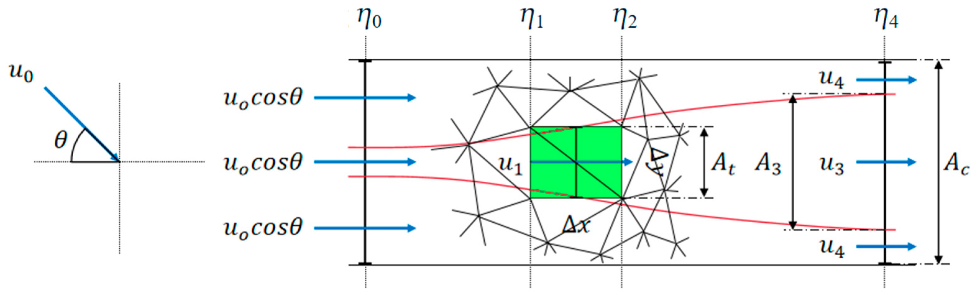
To clarify the relationship between and , the Linear Momentum Actuator disk Theory is adopted. As illustrated in Figure 1, we define a channel with cross-sectional area. The cross-sectional area where a turbine is located is denoted as . In the far downstream region, the velocity in the wake is represented by , corresponding to a cross-sectional area , while the bypass velocity is defined as . It is assumed that a uniform water surface elevation exists at the points where and are defined. The upstream water level is defined as . The water levels just upstream and downstream of the turbine located area are determined by and , which is associated with the turbine, caused a pressure drop. Following the derivation in [23,24], by combining the conservation of mass equations, momentum equations, and Bernoulli equations, the relationship between and is obtained as follows:
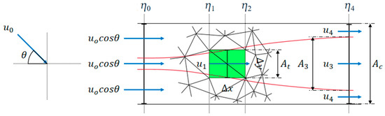
Figure 1.
Schematic diagram of wake velocity analysis for yawed turbines based on actuator disk theory. The green rectangular region in the figure is the grid where the turbine is placed, with bed roughness enhanced to simulate the turbine.
However, in the two-dimensional nonlinear shallow water model of Thetis, turbines are parameterized as regions of enhanced bottom friction. As noted by Kramer and Piggott [23], in a depth-averaged model, the turbine thrust force is actually distributed among a larger region, , than the turbine’s rotation area, . The difference between and is shown in Figure 2. By defining the thrust coefficient of a two-dimensional turbine as , the relationship between and can be expressed as:
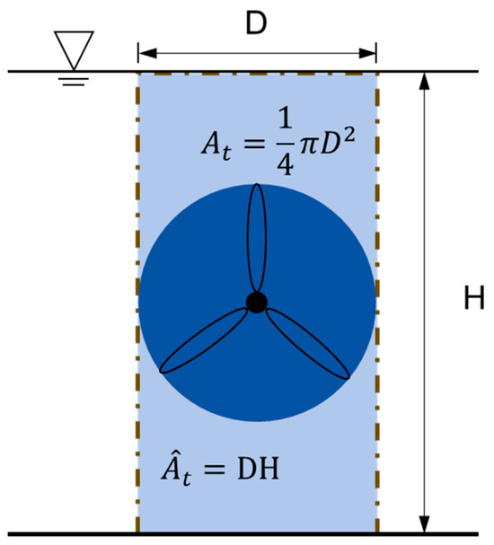
Figure 2.
Schematic diagram of and . The light blue area framed by the dotted line is , and the blue circular area is the swept area of the turbine blades .
Thus, when shallow water equations are the governing equations, Equation (5) should be revised as follows:
Substituting Equations (6) and (7) into Equation (3), the turbine thrust force as a function of and can be expressed as follows:
Equating Equation (8) with Equation (4), the relationship between the dimensionless friction coefficient, and the thrust coefficient, , can be formed as follows:
The power output of a single turbine can be expressed as follows:
The total power output of the array is obtained by summing up the output energy of each turbine:
Although the power output and force of the tidal stream turbine have been simulated, the deflection of the turbine wake is not captured in the two-dimensional model due to the vertical averaging of flow velocity. In order to obtain the wake deflection phenomena, an additional force perpendicular to the incoming flow is added at the turbine location following the method introduced by Zhang et al. [24]. In doing so, the wake deflection can be captured numerically while the turbine power output has not been disturbed. The additional force can be defined as follows:
where is set to 30, the specific derivation of the above formula can be found in [24].
2.3. Economic Evaluation Model
In the construction of a tidal stream turbine array, economic costs are closely linked to the turbine layout, particularly the submarine cables used to transmit electricity generated by turbines to the onshore power station. According to Vazquez et al. [21], submarine cable costs account for more than 10% of the total economic expenditure. Therefore, optimizing the connection sequence is crucial to minimizing the submarine cable length. Moreover, since the capacity of cables for electricity transmission is limited, it is equally important to determine an optimal turbine grouping strategy to ensure that a single cable can efficiently transmit the electricity generated by all the turbines it connects.
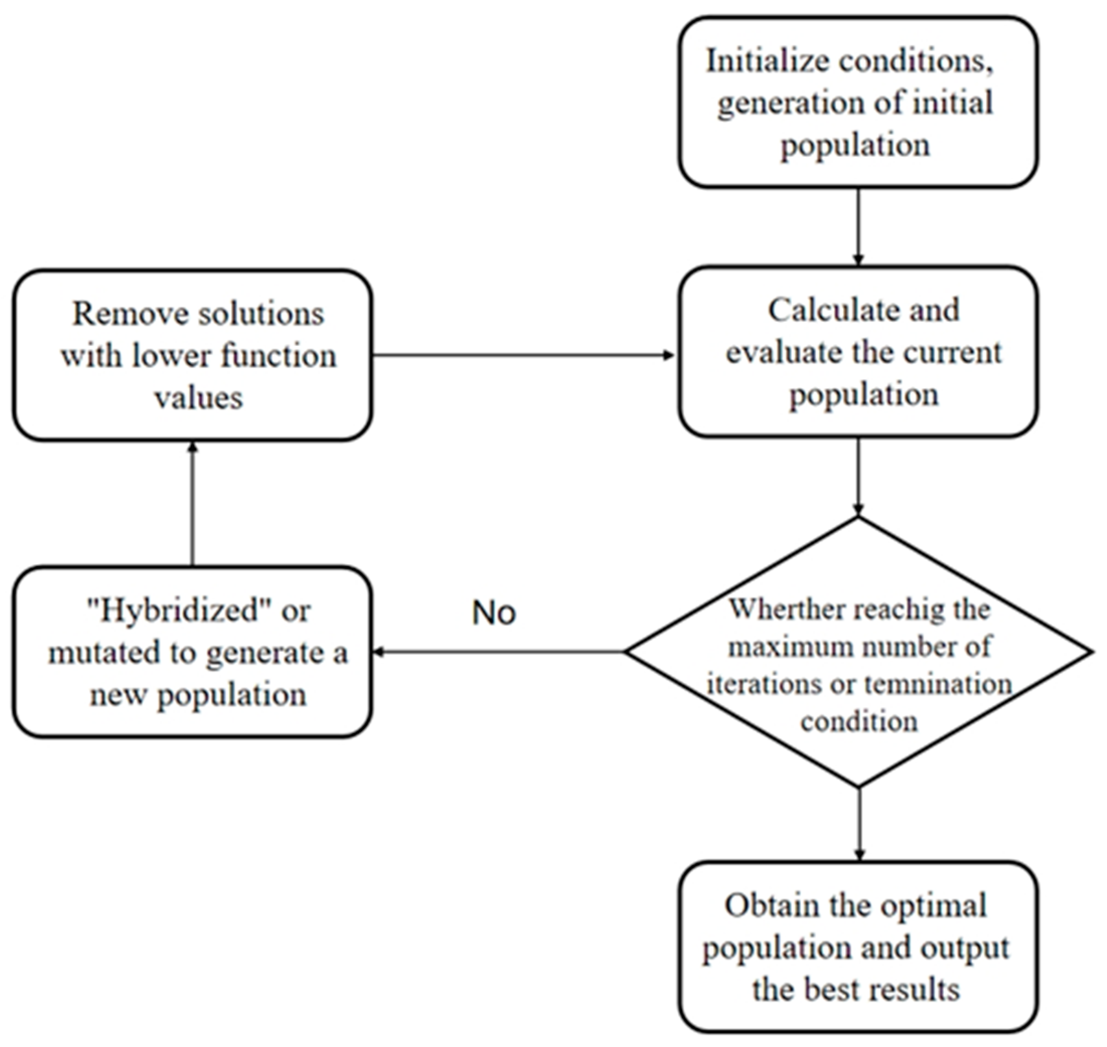
In this paper, the length of submarine cables is considered as the economic indicator. A genetic algorithm (GA) employing a two-stage chromosome structure is used to simultaneously optimize turbine grouping and connection sequence. The effectiveness of this GA method has been demonstrated by Culley et al. [16]. The overall procedure can be summarized as in Figure 3.
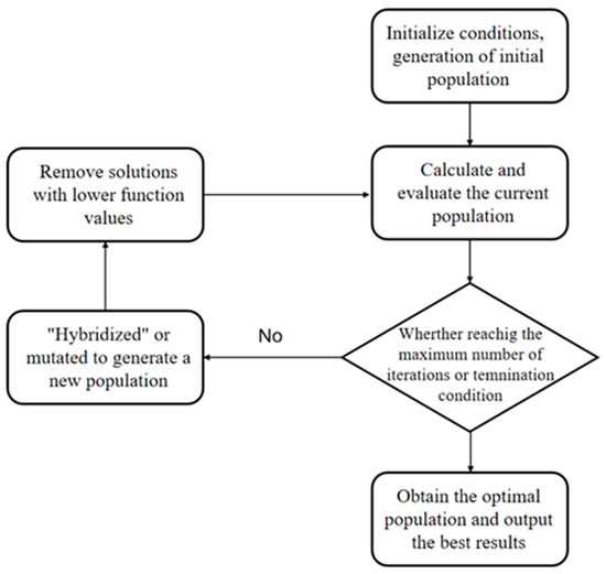
Figure 3.
Sketch map of genetic algorithm process.
Once the grouping of the turbines and the connection sequence are determined, the submarine cable length can be calculated using the following equation:
where mean coordinates of the th tidal stream turbine in the th group, is the number of turbines in the th group, is the number of groups.
2.4. Two-Objective Optimization Function
In this paper, the two-objective optimization, designed to simultaneously maximize array power output and minimize economic cost, is formulated as:
where is the objective function, is a vector containing the coordinates for each turbine, and represent the lower and upper limits of the coordinates, denotes the limitation of the minimum spacing between two tidal stream turbines.
A gradient-based optimization algorithm is adopted in this study, as it takes fewer iterations to reach the optimal result compared with a meta-heuristic algorithm. Since the two-dimensional shallow water equations must be solved in each iteration, fewer iterations can significantly reduce the computational cost. However, a gradient-based optimization algorithm is inherently limited to single-objective optimization. Therefore, to ensure the application of the gradient-based optimization algorithm, array power output and the submarine cable length are linearly combined using two weight coefficients to form a new optimization objective as follows:
where is the objective function; and are the weight coefficients of two objectives, and their sum is 1; is the array power output; is the submarine cable length, is defined as the power output when and , while is defined as the submarine cable length when and .
3. Case Setting
3.1. Computational Domain
The waterway between Putuoshan Island and Huludao Island in Zhoushan City, Zhejiang Province, commonly known as Huludao Water Area (HWA), is selected as the study area to demonstrate the developed optimization framework. The waterway is also the site of the first tidal stream energy demonstration project of China. Therefore, extensive field-measured data, including coastline geometry, bathymetric profiles, and tidal observations, are available and have been utilized for the development and validation of the hydrodynamic model.
The computational domain is shown in Figure 4. The longitude range of the computational domain is 122.26° E to 122.53° E, and the latitude range is 29.89° N to 30.15° N. As shown in Figure 4a, the red rectangular area within the purple enlarged frame is the proposed area where the tidal stream turbines will be deployed. In order to fully capture the impact of the turbine on the tidal stream, the minimum grid cell size at the proposed area is set to 5 m, which is supposed to be less than 1/4 of the turbine diameter. Similar settings can also be found in previous studies [25,26]. The grid size on the land boundary of Putuoshan and Hulu Island is 50 m, and the grid size on other land boundaries is 200 m. The computational domain contains 20,648 grid nodes and 40,492 grid cells. The QMesh software package [27] is used to generate a Gmsh-compatible mesh file for subsequent simulations in Thetis [28].
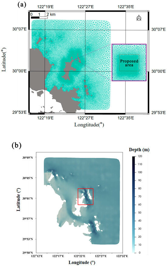
Figure 4.
The computational domain covering the HWA. (a) the mesh, (b) the water depth distribution.
Based on the field-measured data from the first tidal stream energy demonstration project in Zhoushan, the water depth within the computational domain is interpolated, as shown in Figure 4b. The water depth of HWA, as marked by the red rectangle, varies from 20 m to 60 m.
3.2. Boundary Conditions
Adopting the eight primary tidal constituents (Q1, P1, O1, K1, M2, S2, N2, K2) from open-source TPXO9-atlas database [29] to form the tidal forcing on the open sea boundary is a common approach for simulating hydrodynamics around the Zhoushan Islands. However, the spatial resolution of the TPXO9-atlas database is limited to 1/30°, which results in fewer than 20 spatial data points available along the open boundary of the computational domain used in this study. Consequently, the TPXO9-atlas database alone is insufficient for establishing accurate boundary conditions in this case.
To address this limitation, tidal elevation and tidal stream velocity data calculated using a much larger computational domain from [30], in which the use of TPXO9-atlas data is appropriate, are adopted to define the boundary conditions. The simulation case presented in [30] is referred to as Case L, while the simulation case used in this study is referred to as Case S. A comparison of the simulation results from these two cases is provided in Section 4.2.
3.3. Initial Conditions
For the hydrodynamic model, the initial conditions differ between the validation cases and the subsequent study cases. In the validation cases, the initial tidal elevation and tidal stream velocity are uniformly set to zero across the entire computational domain. For the study cases following validation, the initial conditions are derived from the results of the validation simulations by specifying a particular simulation start time.
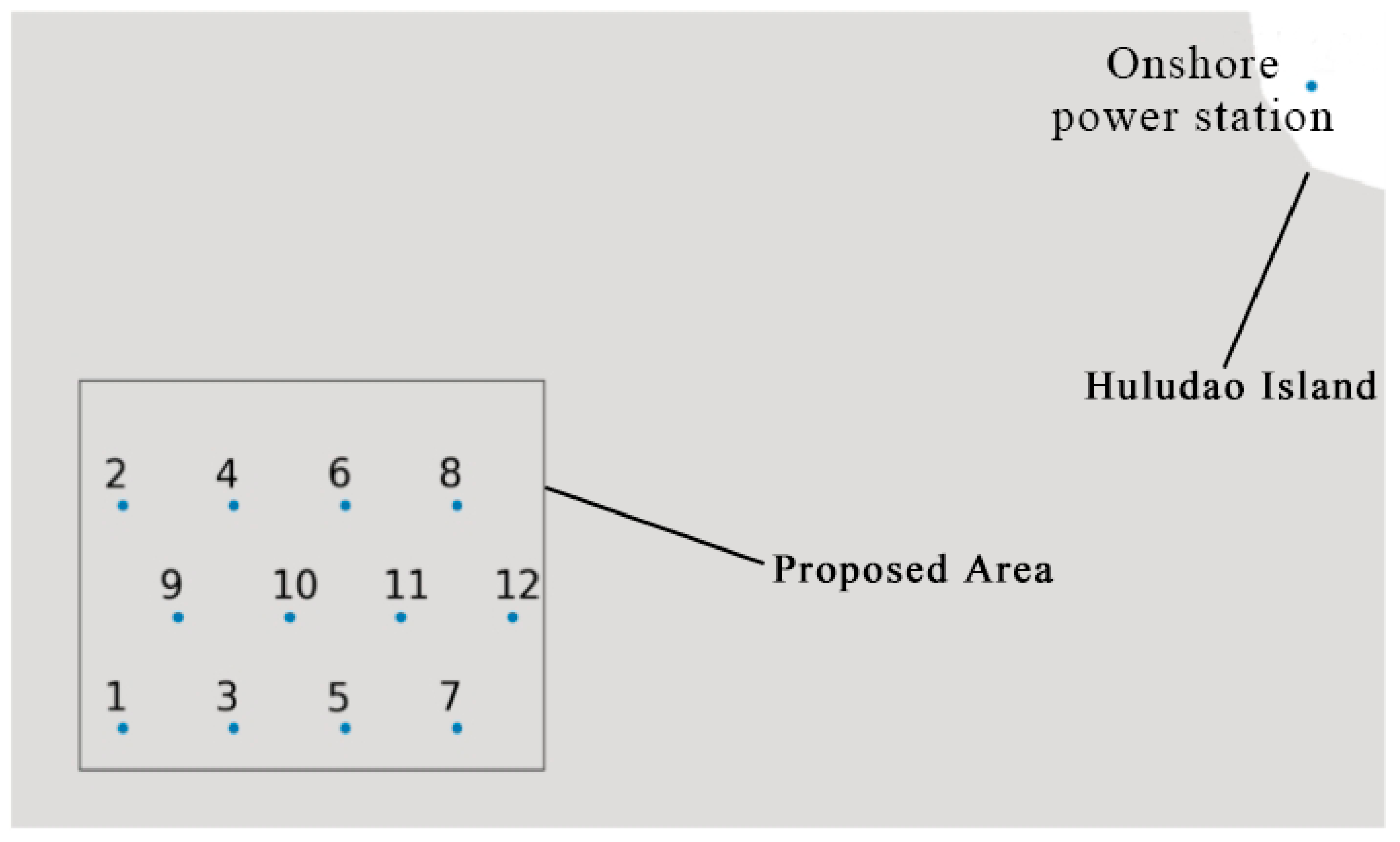
Regarding the turbines, the yaw angles for each turbine are initialized as 0° during the flood tide and 180° during the ebb tide. The initial turbine layout adopts a staggered configuration, as shown in Figure 5.
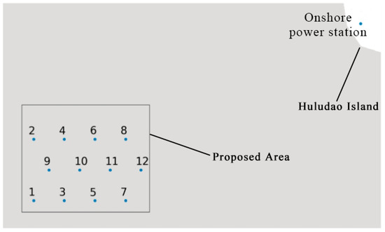
Figure 5.
The location of the onshore power station and the layout of 12 turbines in the array. The numbered blue dots indicate the locations of the turbines.
3.4. Solver Setting
In this study, the shallow water equations are solved using the finite element discontinuous Galerkin method. For the spatial discretization, piecewise-linear discontinuous basis functions (P1DG) are chosen for both the tidal elevation and tidal stream velocity field. For temporal discretization, the backward Euler method is employed with a time step of 5 min. The total simulation time spans 13 h, which starts from 19 August 2013 14:00 and ends at 20 August 2013 03:00, covering a complete semi-diurnal tidal period.
To prevent spurious reflections at the open boundary, a sponge layer with enhanced viscosity and bottom friction is implemented along the boundary. The width of the sponge layer is set to 800 m. Within the sponge layer, the viscosity coefficient ν decreases linearly from 1000 m2/s to 1 m2/s, and remains constant at 1 m2/s throughout the rest of the computational domain.
For all turbines, the rotor diameter is uniformly set to 20 m. The thrust coefficient is assumed to remain constant at 0.6.
3.5. Studying Cases Set Up
In this study, the trade-off between power output and economic cost of a tidal stream turbine array with 12 turbines is investigated. Submarine cables are used to transmit the electricity generated by the turbines to the onshore power station. The total length of the submarine cables is regarded as the economic cost.
Since the electricity transmission capacity of a single cable is limited, the number of turbines connected to one cable is also constrained. This study examines two scenarios regarding the cable capacity. In Scenario 1, each cable supports up to three turbines, while in Scenario 2, this capacity is increased to four turbines.
In both Scenarios, the positions and yaw angles of all turbines are optimized to maximize the power output, while ensuring the shortest submarine cable length by improving the turbine grouping and connection sequences. To investigate the optimal layout differences with varying weight coefficients α and β, six cases are set up for both scenarios:
- (1)
- Case 1:
- (2)
- Case 2:
- (3)
- Case 3:
- (4)
- Case 4:
- (5)
- Case 5:
- (6)
- Case 6:
Among all the cases, 12 tidal stream turbines are initially deployed in the “4-4-4” staggered layout within the proposed area, as shown in Figure 5.
4. Model Validation
4.1. Validation Metrics
Two validation metrics, RMSE (Root Mean Square Error) and the coefficient of determination , are adopted to assess the accuracy of the hydrodynamic model [31,32]. RMSE quantifies the average magnitude of error between model predictions and observed data, with lower values indicating higher accuracy. evaluates the goodness-of-fit between the model outputs and actual observations. The optimal value is 1.0, indicating perfect agreement, while negative values suggest that the model-observation agreement is significantly poor.
The expression of RMSE is as follows:
where and are the th measured data and the th numerical data, respectively; is the total number of measured data.
is expressed as follows:
where is the mean value of the measured results, .
4.2. Hydrodynamic Model Validation
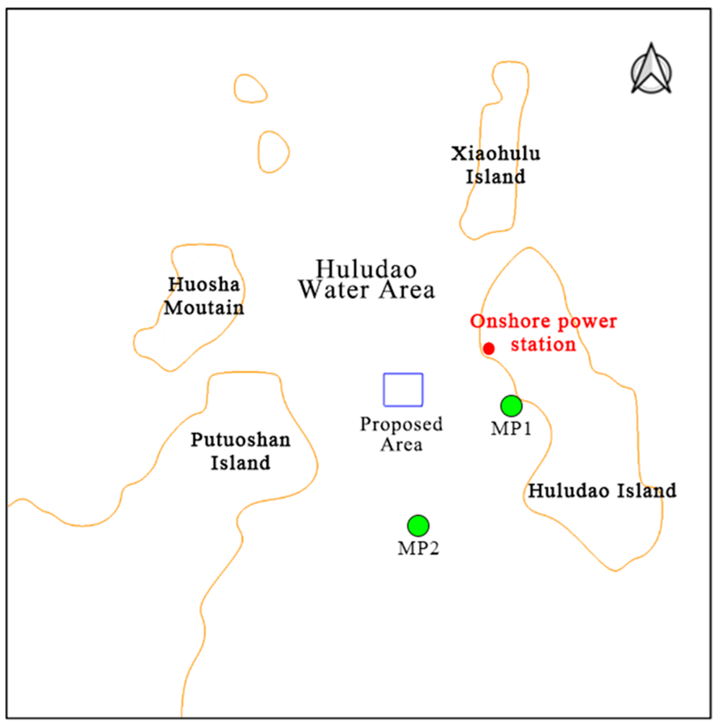
To verify the accuracy of the hydrodynamic model, field measured data from an elevation measuring point MP1 and a velocity measuring point MP2 is collected. The location of two measuring points is shown in Figure 6.
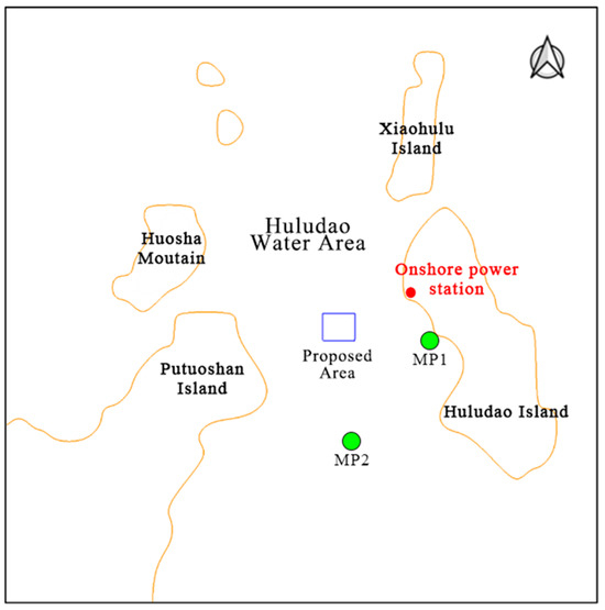
Figure 6.
The location of the measuring points, MP1 and MP2, and the onshore power station within Huludao Water Area.
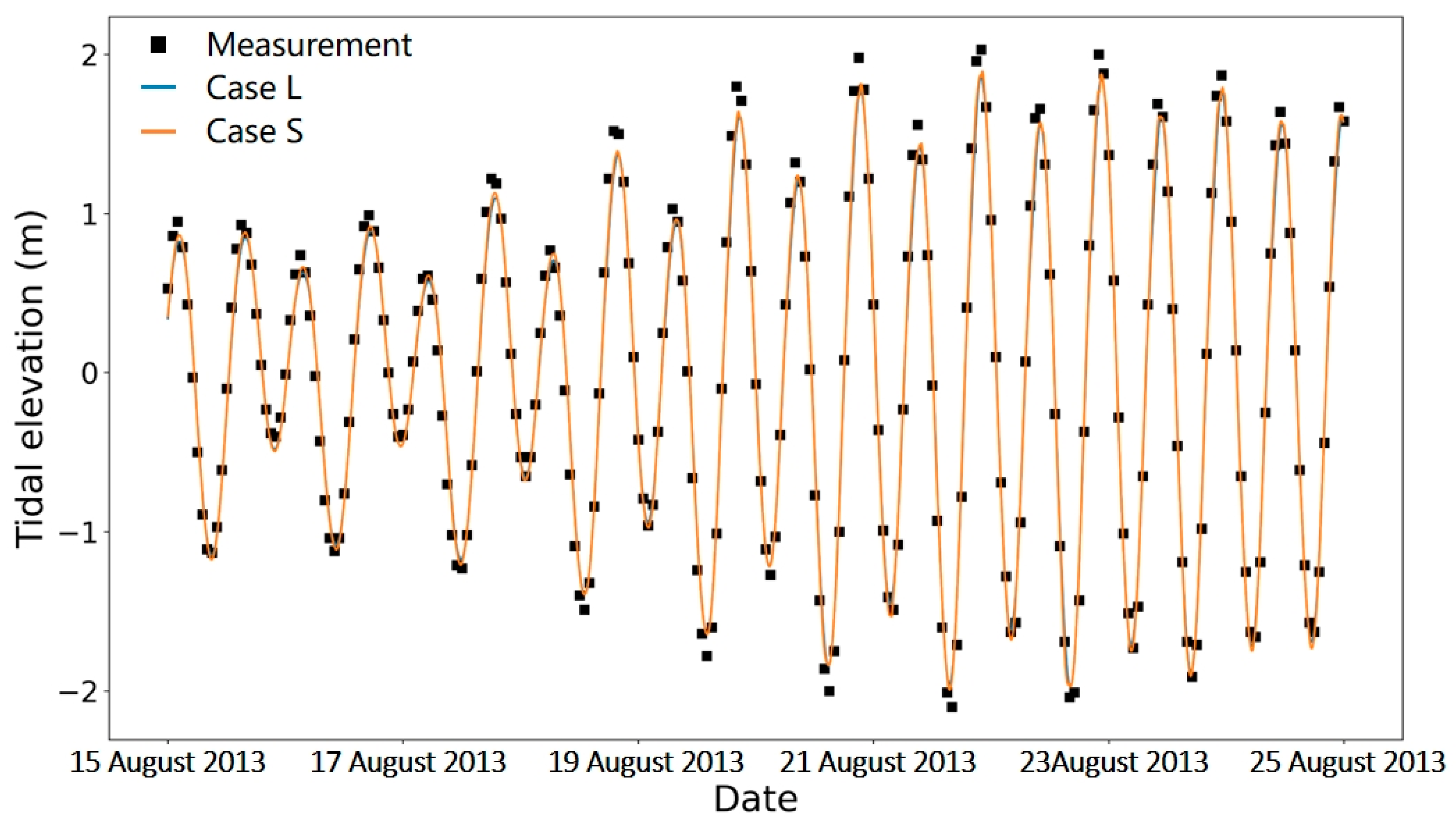
Figure 7 presents a comparison between the simulated tidal process and the measured tidal process. It can be seen that the simulated results from both Case L and Case S exhibit strong agreement with tidal elevation measurement, with negligible deviations at the tidal peak moments. Table 1 presents errors between the simulated and measured values of tidal elevation. As can be seen, the RMSE values of tidal elevation for both cases are extremely low throughout the entire period, at around 0.15 m. The values of are both higher than 0.97, approaching the ideal value of 1.0. These validation metrics confirm the high accuracy and reliability of the simulated tidal elevation results for both cases.
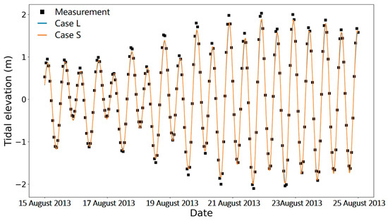
Figure 7.
Comparison between measured and simulated tidal elevation at the measurement point MP1.

Table 1.
Statistical metrics between the simulated results using the computational domain and observed data at stations MP1/MP2.
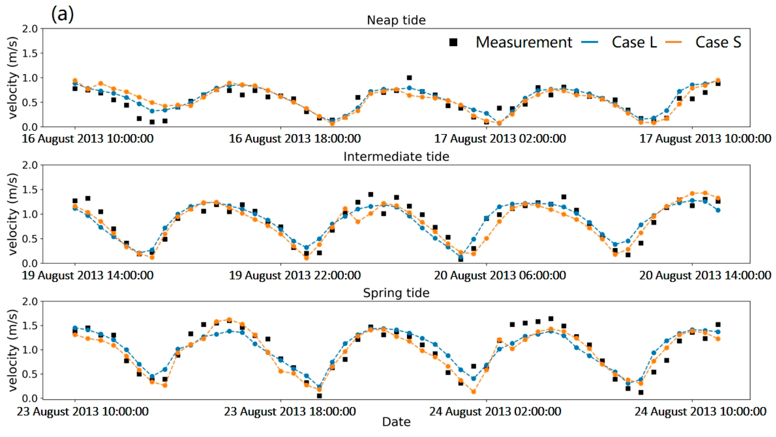
Figure 8a,b compare the simulated and measured tidal flow velocity and flow direction. The results confirm that both Case L and Case S exhibit comparable accuracy in simulating tidal flow velocity, with good agreement observed relative to the field measurements. As shown in Table 1, Case L achieves the lowest RMSE for tidal flow velocity during the neap tide, at 0.126 m/s; however, it also exhibits the highest error in flow direction, reaching 44.3°. In contrast, during the intermediate tide, the RMSE for tidal flow velocity increases slightly to 0.149 m/s, while the error in flow direction decreases significantly. For Case S, the RMSE values for flow velocity during both neap and intermediate tides are nearly identical, at approximately 0.156 m/s. Similarly, the error in flow direction during the intermediate tide is significantly lower than during the neap tide. The largest RMSE in simulated tidal flow velocity for both cases occurs during the spring tide.
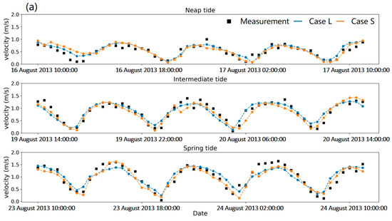
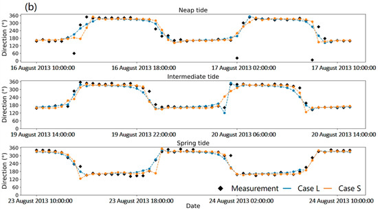
Figure 8.
Comparison between measured and simulated tidal stream velocity at the measurement point MP2: (a) tidal stream velocity magnitude, (b) tidal stream velocity direction.
For the value of , it is computed only for the flow velocity, as averaging flow direction lacks physical meaning. Notably, the for neap tide are the lowest for both Case L and Case S, falling below 0.720. In contrast, during the intermediate and spring tides, the exceed 0.800, indicating a stronger correlation between simulated and observed flow velocities.
In summary, by using tidal elevation and velocity outputs from a large-domain simulation in [30] (Case L) to form the boundary conditions, the smaller computational domain adopted in this study (Case S) achieves simulation accuracy nearly identical to that of the large-domain results reported in [30]. This indicates that the hydrodynamic results obtained in this study are reliable. Among the three tidal periods considered, the simulation of intermediate tide provides the most balanced performance in accurately simulating both tidal elevation and velocity. Therefore, the intermediate tide is selected for subsequent simulations in this study.
It should be noted that although the RMSE for flow direction during the intermediate tide reaches 20.7°, these errors primarily occur during periods when the tidal current reverses direction, during which the flow velocity approaches zero, as shown in Figure 8a,b. Since the primary focus of this study is on predicting turbine power output, which is proportional to the square of the flow velocity, the impact of errors in flow direction during these low-velocity periods is negligible. Thus, the accuracy of the simulated flow direction is deemed acceptable.
The remaining discrepancies in tidal elevation and flow velocity may be attributed to several factors: (1) In Thetis, a uniform Manning coefficient is applied across the entire computational domain, whereas in reality, this coefficient exhibits complex spatiotemporal variations and is neither uniform nor constant. (2) The resolution of the bathymetric data is not high enough to fully capture the steep seabed topography. (3) Wind and other meteorological factors are not considered in the model, despite their potential influence on tidal flow simulation.
4.3. Turbine Model Validation
To validate the accuracy of the yawed turbine model, numerical results are compared with experimental measurements of velocity distribution, as well as with analytically predicted power output and thrust force.
The physical experiment was conducted in the circulating flow flume at Hohai University. The flume is 50 m long, 5 m wide, and 0.7 m deep, as shown in Figure 9. A downward-facing Nortek Vectrino Profiler, mounted on a custom-built rail system for precise movement, is used to collect velocity data within the turbine wake.
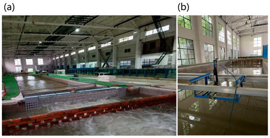
Figure 9.
(a) The circulating flow flume at Hohai University. (b) The downward-facing Nortek Vectrino Profiler.
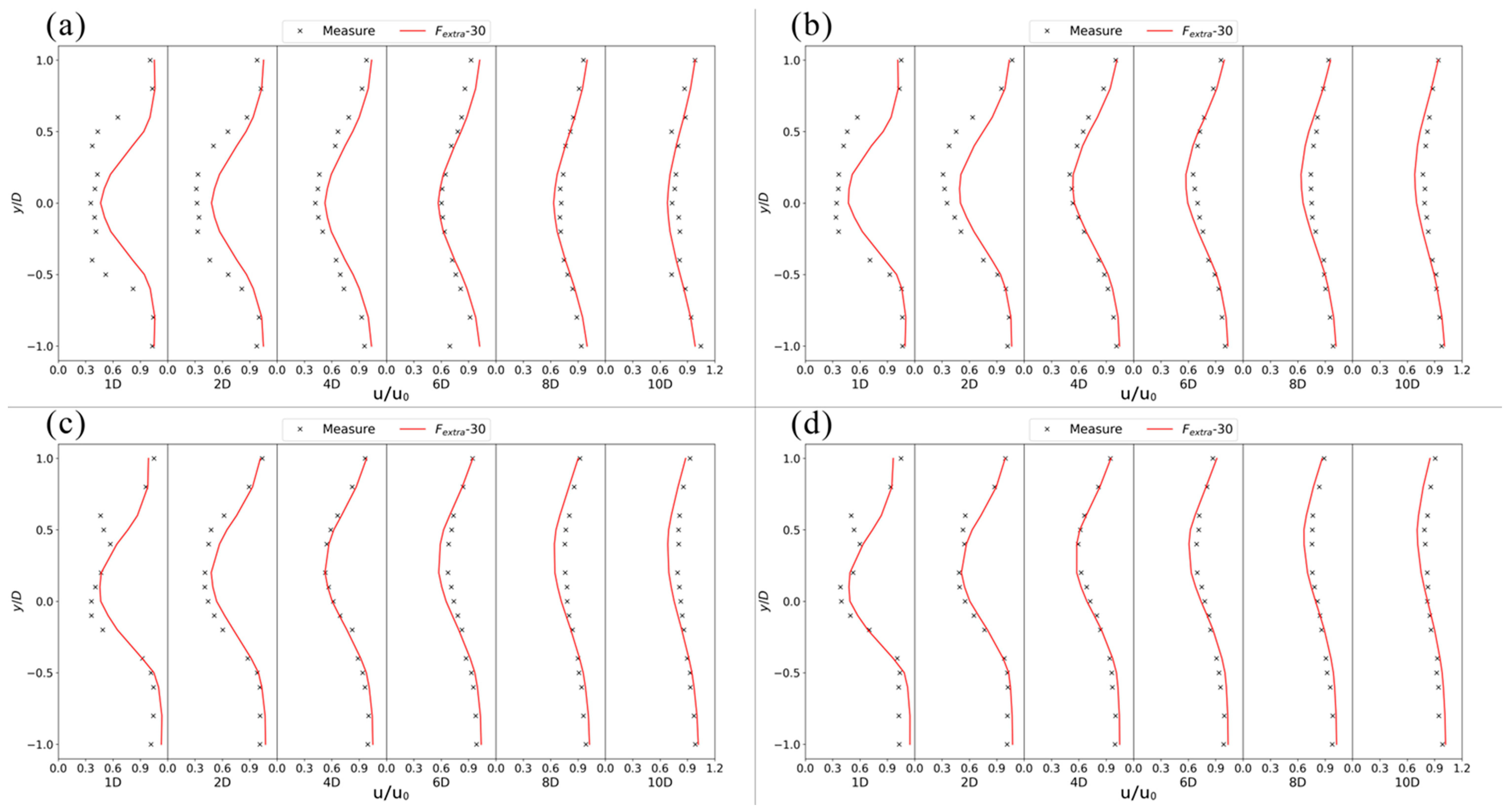
During the experiment, the water depth is set to 0.5 m, the incoming flow velocity to 0.33 m/s, and the turbine diameter to 0.3 m, resulting in an approximate tip speed ratio of 6. The yaw angle of the turbine varies from 0° to 30° in 10° increments. The velocity distribution in the wake is measured at six downstream cross-sections located at distances of 1D, 2D, 3D, 4D, 6D, and 8D from the turbine. At each cross-section, 15 spanwise sampling points are recorded, ranging from y = −1D to y = 1D, with the center of the turbine rotor plane defined as y = 0.
More details about the experiments can be found in [10].
Accordingly, this study establishes a numerical computational domain matching the physical flume dimensions, as shown in Figure 10. This setup enables the numerical simulation of velocity distributions within the turbine wake region under four different yaw angles. The simulated results are then compared with experimental measurements to validate the accuracy of the wake field predicted by the numerical turbine model.
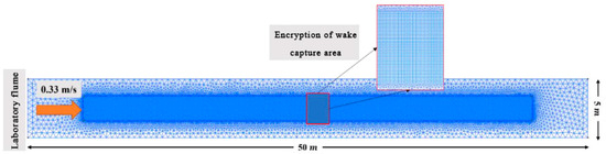
Figure 10.
The computational mesh of the numerical flume, designed with the same dimensions as the circulating flow flume.
Furthermore, the thrust force and the power output of the yawed turbine are validated by comparing the numerical results with the analytical results. The analytical equations of the thrust force and the power output as functions of the inflow velocity are obtained by submitting Equation (7) into Equations (8) and (10), respectively:
where is the area of the turbine’s rotation plane, with the diameter at 20 m. is a rectangular area, the size of which can be calculated as , where is the water depth at 40 m. is the turbine thrust coefficient constant at 0.6. is the incoming velocity constant at 2 m/s, is the yaw angle, which varies from 0° to 90° with a step of 10°.
4.3.1. Validation of Turbine Wake
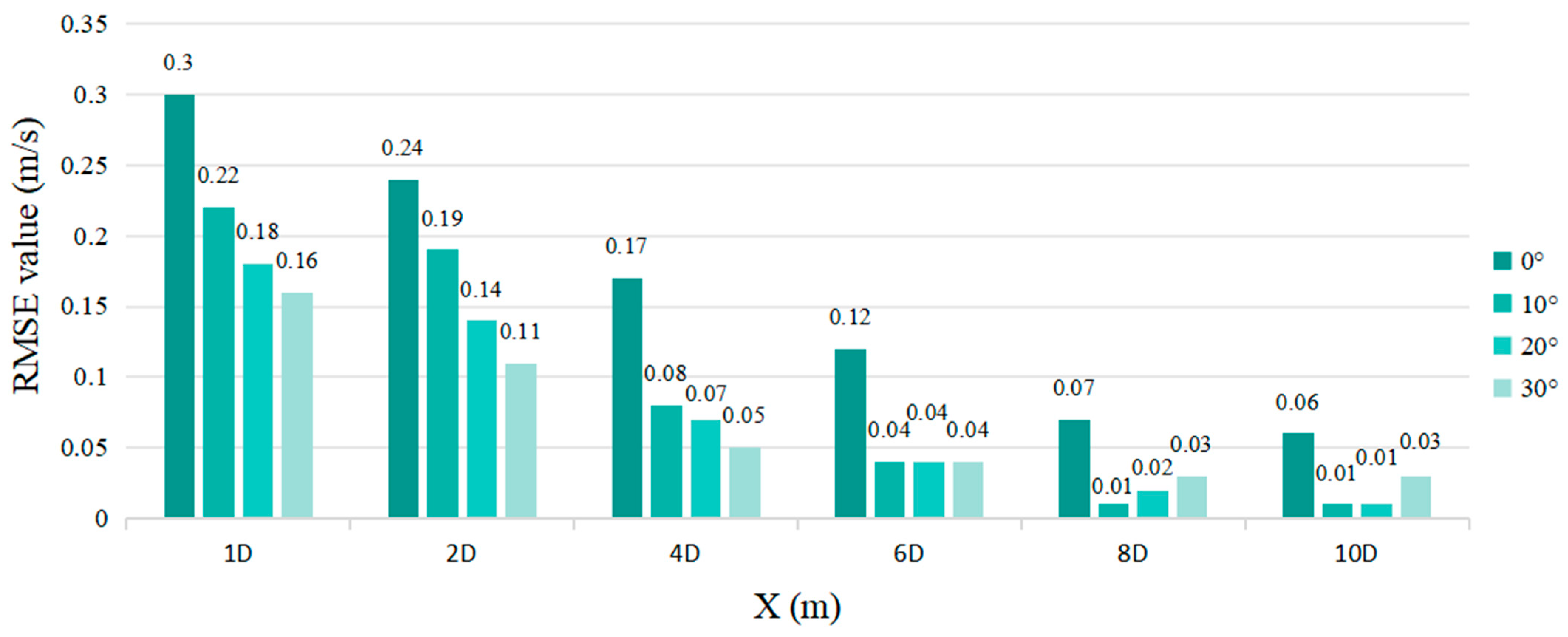
Figure 11 presents the flow velocity validation results for four different yaw angles introduced in Section 3.1. It is evident that in the near-wake region (X/D < 4, where X represents the distance from the measuring point to the tidal stream turbine), numerically predicted flow velocities are slightly higher than the measured values. In the far-wake region (X/D ≥ 4), the numerical simulation results closely align with the experimental measurements. Figure 12 further shows that the RMSE values for all four yaw angles generally remain below 0.10 m/s in the far-wake region. Only when the yaw angle is 0°, does the RMSE exceed 0.10 m/s at both 4D and 6D, which is primarily due to the omission of support structures in the numerical model.
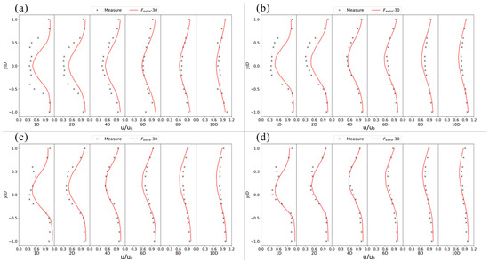
Figure 11.
Verification diagram of flow velocity distribution in each section of the wake field of a single tidal stream turbine at different yaw angles: (a) 0° yaw angle; (b) 10° yaw angle; (c) 20° yaw angle (d) 30° yaw angle.
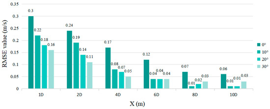
Figure 12.
The RMSE values between the simulated and measured velocity values at each sampling section under different yaw angles.
Despite the discrepancies in near-wake region, the validation results indicate that the turbine model can reproduce the wake field of a yawed turbine effectively. In this study, the minimum spacing between turbines is set to 2D to ensure safe operation, which means the simulation discrepancies in the near-wake region can be neglected in this study, since we only focus on the interaction between turbines with more than 2D distance.
4.3.2. Validation of Turbine Power Output and Thrust Force
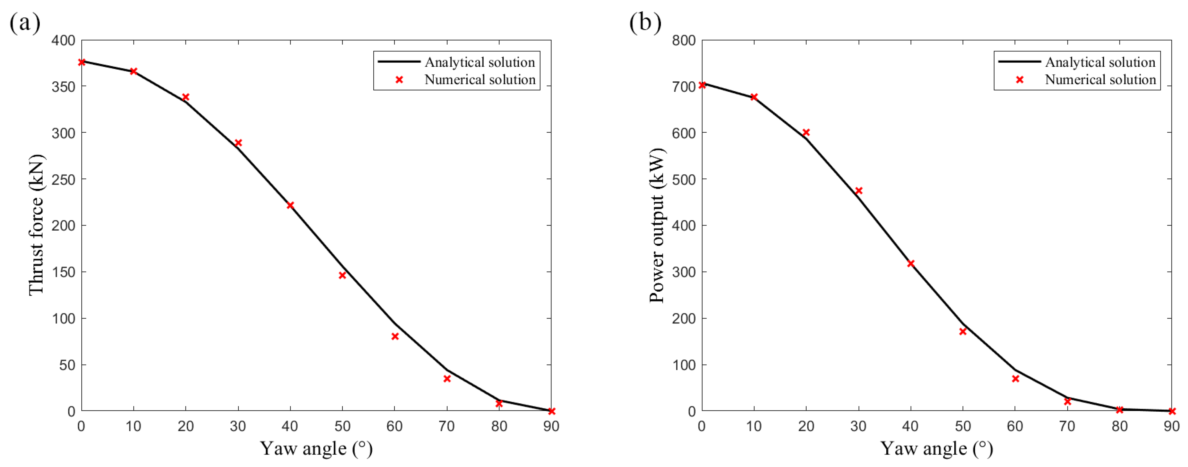
The accuracy of the yawed turbine model is validated by comparing the numerical values of the power output and thrust force against analytical results, which are derived using Equations (18) and (19). The validation results are shown in Figure 13a,b. It is apparent that the simulation results of the yawed turbine model developed in this study exhibit a strong agreement with the analytical results. The RMSE values for thrust force and power output are 6.69 kN and 10.85 kW, respectively. The values are both at 0.998. The values of validation metrics confirm that the accuracy of the simulated turbine power output and thrust force are acceptable.
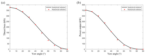
Figure 13.
Comparison of the numerical and analytical results. (a) turbine thrust force, (b) turbine power output.
4.4. Optimization Model Validation Results
4.4.1. Validation of the Gradient-Based Model
In order to ensure the reliability of gradient-based algorithms, this paper verifies the accuracy of the gradient value of the objective function, using the remainder term of the second-order Taylor expansion. The second-order Taylor expansion of is expressed as follows:
where is the disturbance in any direction, and in this model, it is the gradient direction. is the disturbance ratio coefficient that controls the magnitude of disturbance, and in this model represents the step size in the gradient direction.
During program execution, the function value and its derivative are computed through the adjoint method [25,33]. By assuming an arbitrary fixed value of , the second-order residual can be determined according to Equation (20). Based on the prior experience, the residual value decay rate is generally required to exceed 1.95 [8]. In all subsequent calculations, this criterion is ensured.
4.4.2. Validation of the Genetic Algorithm
The genetic algorithm is a gradient-free optimization algorithm method, requiring only that it consistently converges to the same optimal solution within the specified number of iterations.
The population size and the number of generations are two of the key parameters of genetic algorithms. The increase in these two parameters prolongs calculation time but enhances solution accuracy. Therefore, in order to balance the calculation cost and the accuracy of the calculation results, appropriate genetic algorithm parameters should be chosen. To determine the optimal values of the genetic algorithm parameters, this section takes the 12 turbines in the initial condition as an example. The locations of each turbine and the onshore power station are shown in Figure 5.
As shown in Table 2, regardless of the cable capacity, varying the maximum number of iterations does not affect the optimal results and has a negligible impact on the computation time. This suggests that the genetic algorithm converges before reaching the maximum number of iterations in each group, as evidenced by the consistency of the final 20 optimization results. However, when the initial population size increases, a noticeable rise in computation time is observed. For every additional 2000 individuals in the initial population, the computation time increases by approximately 4 s.
Table 2.
The optimization results and computation time for different initial population sizes and different maximum iteration numbers.
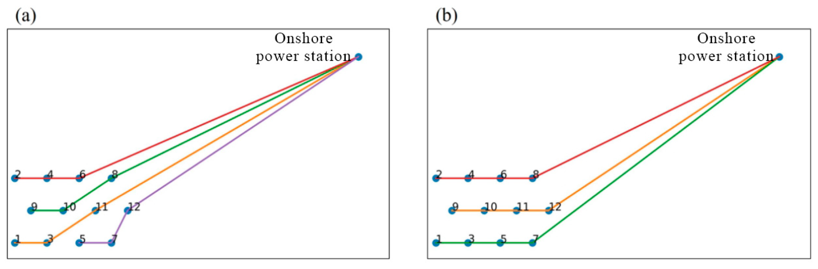
In terms of calculation accuracy, when the initial population size is set to 1000, the genetic algorithm yields local optimal solutions. When the initial population size is larger than 1000, the global optimal solution is successfully identified by the genetic algorithm. The shortest submarine cable lengths reach 2745.71 m and 2144.55 m for the two different cable capacities, respectively, as shown in Figure 14.
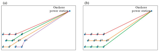
Figure 14.
The optimal linking between inland electrical station and turbines: (a) maximum linking number per cable is 3, (b) maximum linking number per cable is 4. The numbered blue solid dots represent the turbines. The red, green, yellow, and purple lines represent four submarine cables.
In summary, when the array consists of 12 tidal stream turbines, the size of the initial population significantly influences the final outcomes and computation time of the genetic algorithm, whereas the maximum number of iterations has negligible impact. Consequently, to ensure computational accuracy and save computational cost, the subsequent chapters will set the initial population size to 5000 individuals and the maximum number of iterations to 1000.
5. Results and Discussion
5.1. Results of Scenario 1
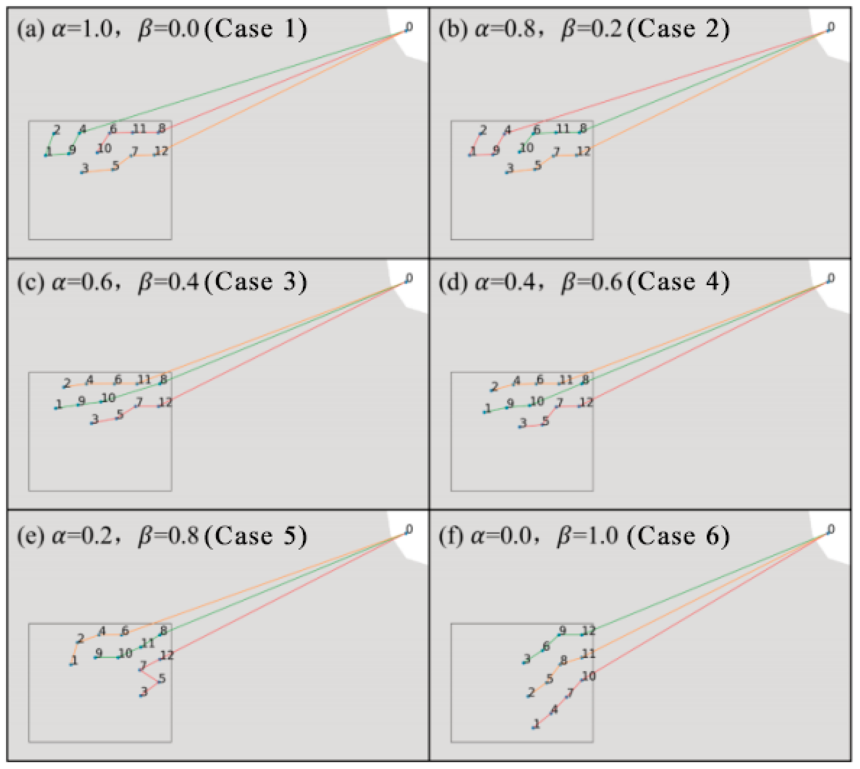
Figure 15 displays the optimal layout of the turbine array and the corresponding optimal cable connection sequence for the six cases of Scenario 1, when the cable capacity is 3 turbines. As can be seen in Figure 15, when the optimization prioritizes maximizing array power output without accounting for submarine cable length, the spacing in east–west direction between the turbines reaches its maximum. This substantial lateral spacing is advantageous as it enables the front row of turbines to effectively extract tidal energy while enabling the staggered arrangement of the back row of turbines to face undisturbed incoming flow, thereby enhancing overall capacity efficiency.
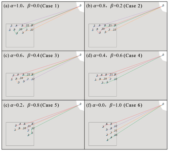
Figure 15.
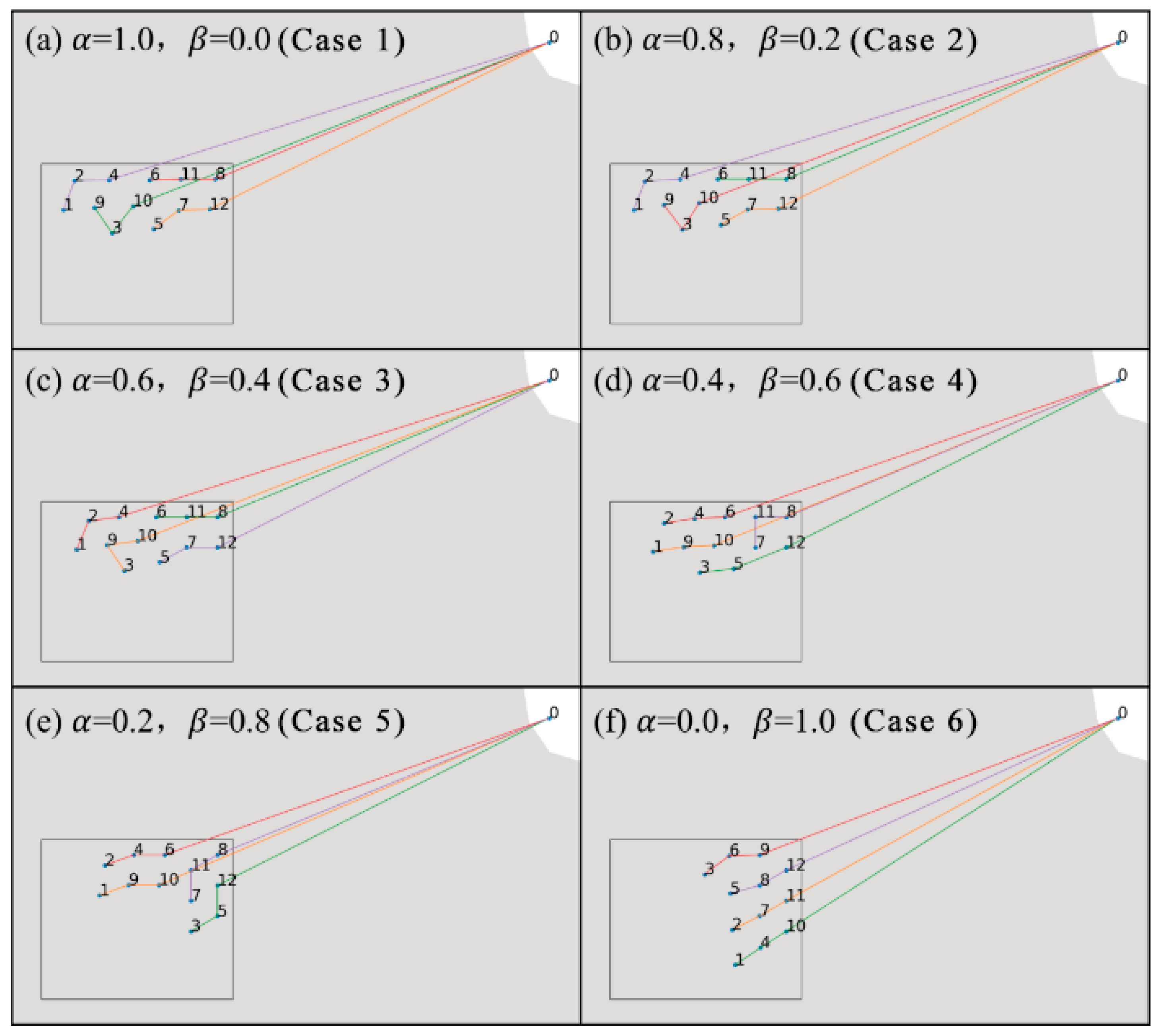
The schematic diagram of the optimal turbine array layout and the optimal connection sequence of submarine cables with varying weight coefficients and when one submarine cable is capable of linking 3 turbines. The blue dot numbered 0 represents the onshore power station, while the dots numbered 1 to 12 represent the turbines. The red, green, yellow, and purple lines represent four submarine cables.
As the value of decreases and increases, the objective of reducing economic cost exerts a greater influence on the array layout. As depicted in Figure 15b–d, it can be observed that to minimize submarine cable length, the entire array shifts eastward, moving closer to the onshore power station. However, to maximize the total power output, the array layout remains almost unchanged.
In Figure 15e, when reaches 0.8, the entire array contracts toward the northeast corner of the proposed area, leading to a substantial reduction in lateral spacing between the turbines. The turbines connected by the green and purple lines become tightly clustered, significantly affecting the efficiency of each turbine. In contrast, the turbines connected by the red and yellow lines maintain a relatively dispersed layout, maintaining the array’s total power output.
Finally, in Figure 15f, when α is reduced to 0.0, the dual-objective optimization function simplifies to a single-objective optimization function that prioritizes minimizing the length of the submarine cables. In this case, the four turbines directly connected to the onshore power station are positioned near the northeast corner of the proposed area, with a minimum spacing of 40 m between them. Similarly, for turbines connected by the same submarine cable, the spacing between adjacent turbines is also 40 m.
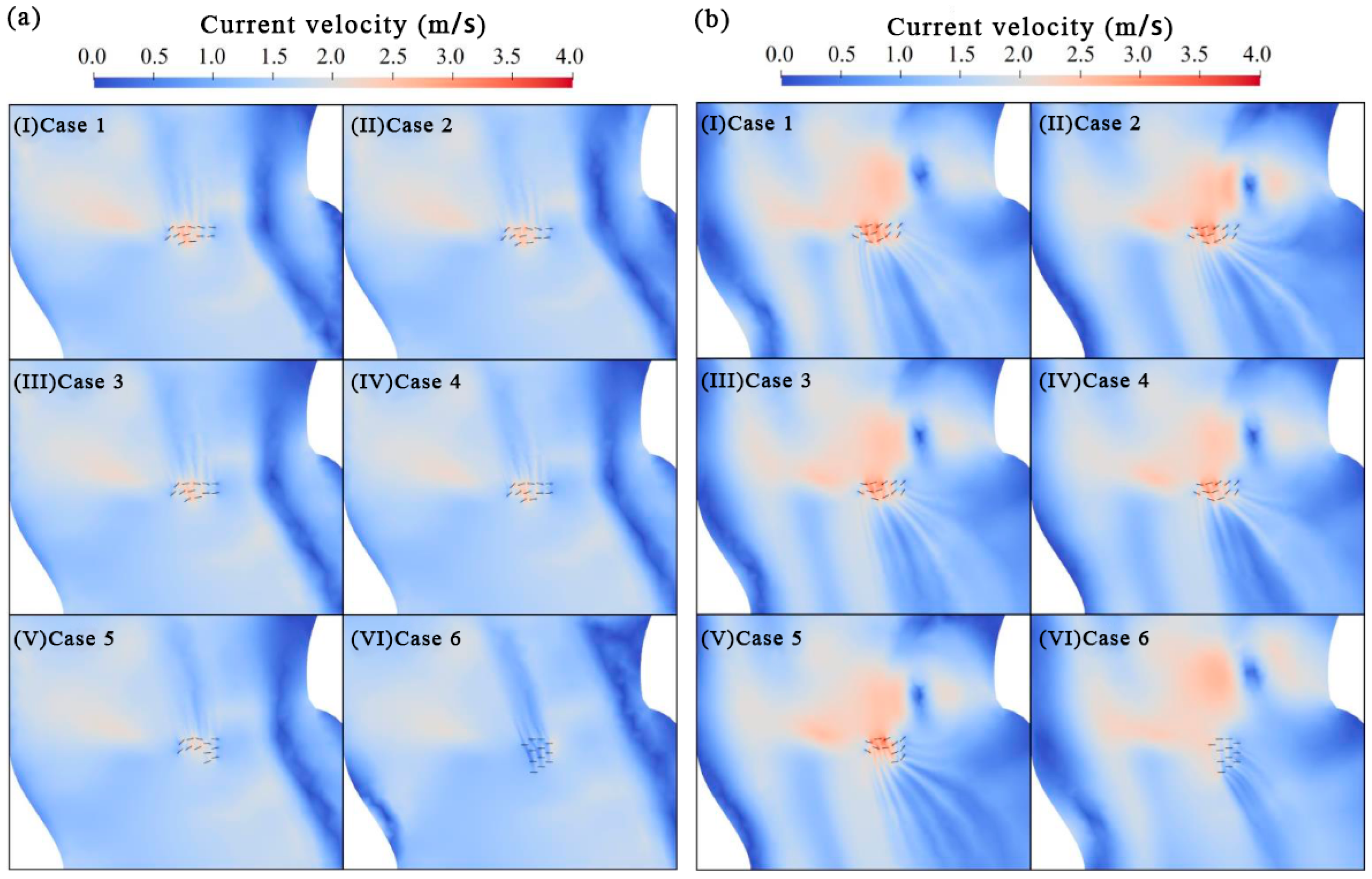
Figure 16 displays the yaw condition for each turbine and the velocity distribution around the turbine array among the six cases of scenario 1. As can be seen, in Cases 1–5, turbines are optimized to be deployed in a “5-5-2” layout during the spring tide and a “2-5-5” layout during the ebb tide. Compared with the initial “4-4-4” layout, the optimized array increases the maximum number of turbines per row from four to five. Regardless of whether it is a spring tide or ebb tide, at least five turbines in the array always face the undisturbed tide. The remaining two turbines are positioned in regions where the flow velocity is accelerated, specifically, in the middle of the array (Cases 1–4) when α is greater than or close to the . Additionally, among these five cases, turbines on both sides operate under yawed conditions, reducing wake interference on downstream turbines and enhancing flow toward the turbines in the center of the array, thereby sustaining power output as much as possible. However, when is significantly larger than , as in Case 5, these two turbines shift eastward to minimize submarine cable length, despite a reduction in power output.
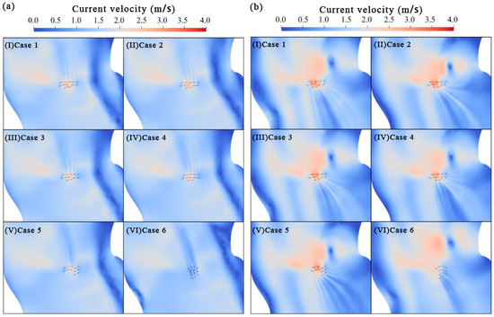
Figure 16.
The schematic diagram of the yaw condition for each turbine and the velocity distribution around the turbine array in 6 cases of scenario 1. (a) at the peak of spring tide, (b) at the peak of ebb tide.
In Case 6, the optimization process focuses exclusively on minimizing submarine cable length, causing all turbines to cluster at the minimum allowable spacing. Furthermore, since the objective of optimizing total power output is disregarded, the yaw angle of each turbine remains at its initial value of zero degrees, leading to a distinctive velocity distribution around the turbine array.
5.2. Results of Scenario 2
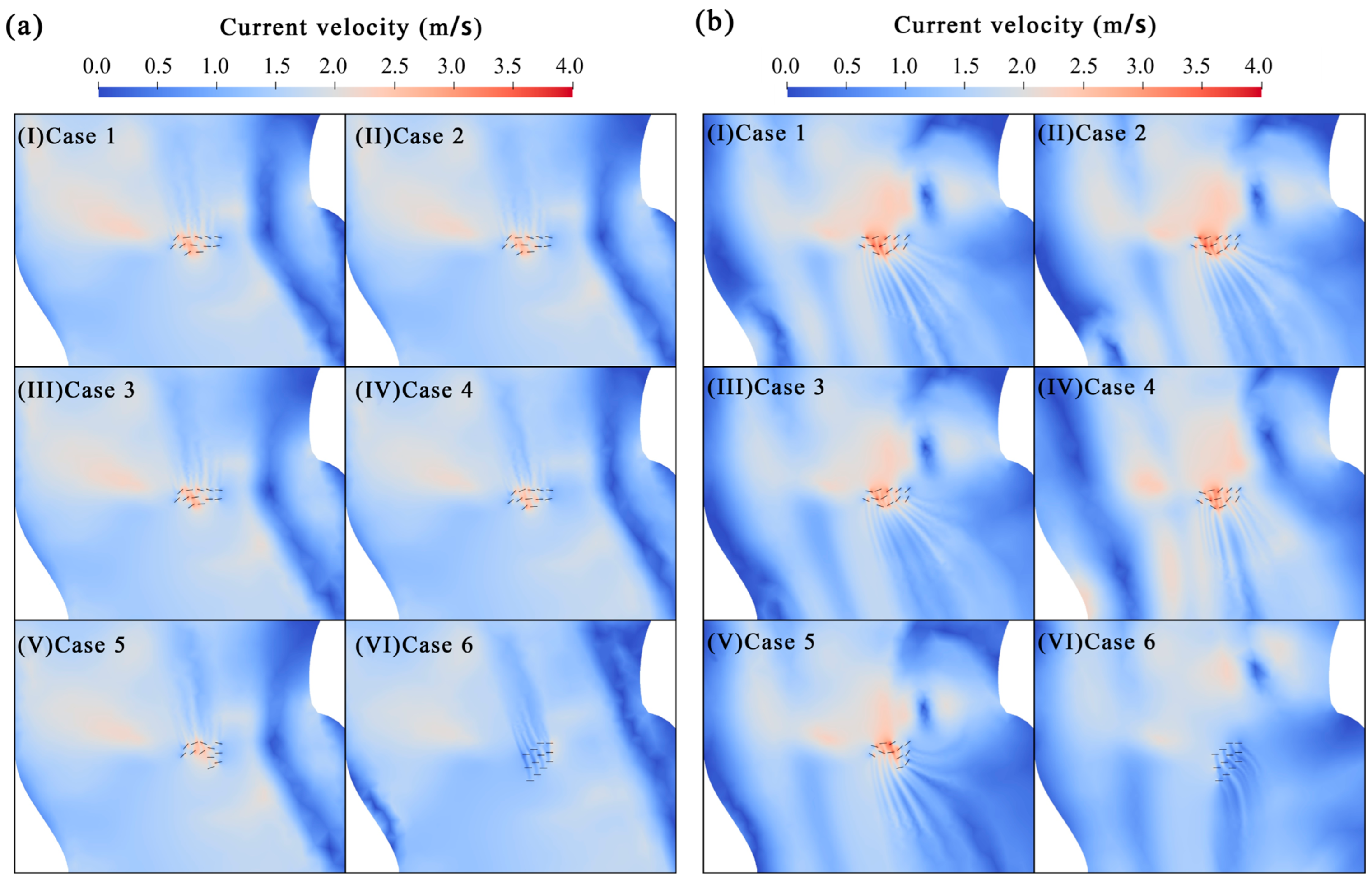
Figure 17 shows the optimal layout configurations for the turbine array across six different cases of Scenario 2. Since minimizing the submarine cable length is not considered in Case 1 of Scenario 2, as shown in Figure 17a, the layout optimization prioritizes maximizing power output, resulting in an array configuration identical to that of Case 1 in Scenario 1.
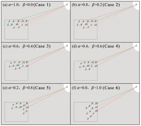
Figure 17.
The schematic diagram of the optimal turbine array layout and the optimal connection sequence of submarine cables with varying weight coefficients and when one submarine cable is capable of linking 4 turbines. The blue dot numbered 0 represents the onshore power station, while the dots numbered 1 to 12 represent the turbines. The red, green, yellow, and purple lines represent four submarine cables.
From Cases 2 to 4, as the weight coefficient for power output () decreases and the weight coefficient for economic cost () increases, the objective of minimizing submarine cable length leads to a reduction in turbine spacing across cases. This progressive increase also causes the turbines directly connected to the onshore power station to shift northeast, moving closer to the onshore power station. Nevertheless, the overall configuration of the turbine array remains largely unchanged compared to Case 1, as the established array layout enhances the array’s total power output.
In Cases 5 and 6, as the priority of reducing submarine cable length increases, the array layout undergoes more significant changes. The three turbines directly connected to the onshore power station are relocated as close as possible to the northeast corner of the proposed area, with the spacing between turbines reduced to the minimum allowable distance. Again, Case 6 remains an uncommon scenario from an engineering perspective, as the objective of improving the array’s total power output is entirely disregarded.
Figure 18 shows the yaw condition for each turbine and the velocity distribution around the turbine array among the 6 cases of Scenario 2. As can be seen, except for Case 6, the turbine layouts in the other cases remain generally similar due to the objective of maximizing total energy output. In general, the array layouts in Cases 1–5 retain the “5-5-2” configuration during the spring tide and the “2-2-5” configuration during the ebb tide, ensuring that the maximum number of turbines face the undisturbed tide. The turbines on both sides also operate under yawed conditions to enhance the efficiency of downstream turbines, particularly the two remaining turbines in the third row.
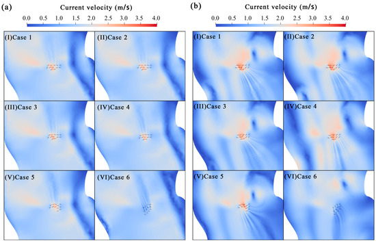
Figure 18.
The schematic diagram of the yaw condition for each turbine and the velocity distribution around the turbine array in 6 cases of Scenario 2. (a) at the peak of spring tide, (b) at the peak of ebb tide.
Although the turbine layout structure changes slightly, the entire array has noticeably shifted toward the center of the proposed area. This shift occurs because the increased cable capacity allows more turbines to be connected to a single cable, enabling greater spacing between turbines to reduce internal interactions and improve total power output. In Case 6, all turbines maintain a yaw angle of 0 degree since only the total submarine cable length is considered, which again results in a significantly different flow field around the turbine array.
5.3. Comparing Scenario 1 to Scenario 2
Table 3 presents the array power output and submarine cable length for the turbine array across six cases of scenarios 1 and 2. The results reveal a systematic decrease in as the weight coefficient βincreases, reflecting the trade-off between power output maximization and cable length minimization. It is evident that the array power output in Scenario 2 consistently surpasses that of Scenario 1. The largest gap shows up in Case 4, where the of Scenario 1 is 16.8% less than that of Scenario 2. The gaps among other cases all reach around 6%, except for Case 6, which is meaningless when comparing the as stated in previous sections. The key reason for the gap is that the increased cable capacity in Scenario 2 enables more turbines to be connected to a single cable and allows the turbines to be positioned closer to the center of the waterway, where tidal energy resources are more abundant, resulting in higher power generation compared to Scenario 1. Furthermore, from Case 1 to Case 5, in Scenario 1 decreases by 24.2%, while in Scenario 2, the reduction is 19.7%, which is 4.5% lower than in Scenario 1. This lower decrement in Scenario indicates that higher cable capacity mitigates the sensitivity of the on .
Table 3.
Array power output and submarine cable length with varying weight coefficients and when the cable capacity is 3 or 4 turbines.
As for the submarine cable length, the value decreases by 183.26 m from Case 1 to Case 6 in Scenario 1. While, in Scenario 2, as cable capacity increases from three to four turbines, the value reduces by 134.00 m, which is 49.26 m less than the corresponding reduction in Scenario 1. It is indicated that the minimization of submarine cable length is more significant when the cable capacity is low.
Furthermore, the submarine cable length in Scenario 2 is significantly lower than that in Scenario 1, dropping from approximately 2400 m to around 1900 m. This significant reduction is primarily attributed to the cables connected to the onshore power station which constitutes over 90% of the submarine cable length. Therefore, the fewer number of the cables leads to the lower submarine cable length in Scenario 2 compared to Scenario 1.
To better understand the effect of the weight coefficient on the changing trend of and , these two parameters are both normalized using the corresponding values in Case 1 of the two scenarios, which are shown as follows:
where is the submarine cable length in Case 1, is the array power output in Case 1.
Figure 19 shows the changing trend of the dimensionless array power output and the dimensionless submarine cable length with the weight coefficient in both scenarios. As can be seen, in both scenarios, the dimensionless submarine cable length decreases linearly with the increase of , with a slope of around 0.645. This indicates that the variation in the cable capacity in the connecting turbines has little influence on the change trend of with .
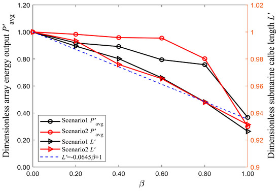
Figure 19.
The changing trend of dimensionless array power output and the dimensionless submarine cable length with the weight coefficient when one submarine cable is capable of linking 3 turbines and 4 turbines.
In terms of the array power output , it exhibits a stepwise decline trend in both scenarios. In Scenario 1, there is a tipping point when after which the drop dramatically with the increase in . For Scenario 2, the tipping point moves to , after which an even more significant reduction is shown for the variation of with . Since the varies in a stepwise trend while changes linearly, the tipping point reveals the best values of for each scenario, where the highest profit is achieved as the economic cost reduces while the power output remains nearly unchanged.
6. Conclusions
This study establishes a two-objective optimization model for a tidal stream turbine array based on the open-source ocean numerical modeling framework Thetis. The yawed turbine model is integrated into the hydrodynamic model, to examine the influence of the wake offset on turbine array layout. The gradient-based optimization model is employed to study the trade-off between the two optimization objectives: array power output and submarine cable length, which represents the economic costs of the turbine array. During the layout optimization, the optimal turbine grouping and connection sequence are determined through a genetic algorithm aimed at minimizing submarine cable length.
The Huludao Water Area is selected as the study area. Two scenarios considering different cable capabilities are analyzed. In each scenario, six cases are examined to investigate the characteristics of the optimized array layout with varying weight coefficients for the two optimization objectives.
In Scenario 1, incorporating economic cost results in a more clustered arrangement of the turbines and a shifting of the entire array towards the onshore power station. The tendency for turbines to be arranged in a single row becomes more pronounced. In Scenario 2, the cable capacity increases from 3 to 4. The overall array layout remains similar to that in Scenario 1, but is positioned closer to the river center.
In both scenarios, when the economic weight coefficient increases, the submarine cable length almost linearly decreases, while the power output declines with a stepwise pattern. Thus, the tipping point in the change trend of array power output indicates where the optimal profit region lies. For example, in Scenario 2, Case 4 represents the tipping point among the six cases and yields the highest overall profit. Furthermore, a comparison between the two scenarios reveals that a larger cable capacity is more likely to result in higher profit. This also suggests that the results of multi-objective optimization are more applicable to engineering than those of single-objective optimization.
It should be noted that although this study focuses on optimizing the turbine array layout within the Huludao Water Area, the proposed model can be readily applied to other water areas, once the essential input data, such as open boundary tidal forcing, coastline geometry, and bathymetry, are available.
While the hydrodynamic and turbine models demonstrate acceptable accuracy in simulating tidal flow and yawed turbine performance, it is important to acknowledge that three-dimensional turbulence effects are not considered due to the use of shallow water equations as the governing model. Previous studies have shown that three-dimensional turbulence can significantly influence the wake characteristics of tidal turbines [34,35,36]. Therefore, future research should incorporate these effects into turbine array layout optimization when computational methods and resources allow.
In addition, due to the confidentiality of detailed economic data, the economic cost in this study is primarily represented by the total length of submarine cables. As a result, the objective function is formed by two factors linked with two weight coefficients. In future work, the availability of more detailed economic information would enable the adoption of more representative objective functions, such as the Levelized Cost of Energy (LCOE) [37], to improve the robustness of the optimization process.
Author Contributions
Conceptualization, C.Z., J.Z., and X.C.; methodology, C.Z.; software, C.Z.; validation, C.Z. and Y.Z.; formal analysis, Z.D.; investigation, Z.D.; resources, X.L.; data curation, C.Z.; writing—original draft preparation, C.Z. and Y.Z.; writing—review and editing, X.C. and X.L.; visualization, Y.Z.; supervision, J.Z.; project administration, C.W.; funding acquisition, J.Z. All authors have read and agreed to the published version of the manuscript.
Funding
This research was funded by the National Key Research and Development Program of China, grant number No. 2023YFB4204102.
Data Availability Statement
Data is contained within the article.
Conflicts of Interest
The authors declare no conflicts of interest. The funders had no role in the design of the study; in the collection, analyses, or interpretation of data; in the writing of the manuscript; or in the decision to publish the results.
Abbreviations
The following abbreviations are used in this manuscript:
| GA | Genetic Algorithm |
| HWA | Huludao Water Area |
| RMSE | Root Mean Square Error |
| LCOE | Levelized Cost of Energy |
References
- Nash, S.; Phoenix, A. A Review of the Current Understanding of the Hydro-Environmental Impacts of Energy Removal by Tidal Turbines. Renew. Sustain. Energy Rev. 2017, 80, 648–662. [Google Scholar] [CrossRef]
- Liu, H.; Ma, S.; Li, W.; Gu, H.; Lin, Y.; Sun, X. A Review on the Development of Tidal Current Energy in China. Renew. Sustain. Energy Rev. 2011, 15, 1141–1146. [Google Scholar] [CrossRef]
- Li, Z.; Li, G.; Du, L.; Guo, H.; Yuan, W. Optimal Design of Horizontal Axis Tidal Current Turbine Blade. Ocean Eng. 2023, 271, 113666. [Google Scholar] [CrossRef]
- Zhu, F.; Ding, L.; Huang, B.; Bao, M.; Liu, J.-T. Blade Design and Optimization of a Horizontal Axis Tidal Turbine. Ocean Eng. 2020, 195, 106652. [Google Scholar] [CrossRef]
- Vennell, R.; Funke, S.W.; Draper, S.; Stevens, C.; Divett, T. Designing Large Arrays of Tidal Turbines: A Synthesis and Review. Renew. Sustain. Energy Rev. 2015, 41, 454–472. [Google Scholar] [CrossRef]
- Tan, J.; Wang, S.; Yuan, P.; Wang, D.; Ji, H. The Energy Capture Efficiency Increased by Choosing the Optimal Layout of Turbines in Tidal Power Farm. In Energy Solutions to Combat Global Warming; Zhang, X., Dincer, I., Eds.; Springer International Publishing: Cham, Switzerland, 2017; pp. 207–226. ISBN 978-3-319-26950-4. [Google Scholar]
- Gauvin-Tremblay, O.; Dumas, G. Hydrokinetic Turbine Array Analysis and Optimization Integrating Blockage Effects and Turbine-Wake Interactions. Renew. Energy 2022, 181, 851–869. [Google Scholar] [CrossRef]
- Funke, S.W.; Farrell, P.E.; Piggott, M.D. Tidal Turbine Array Optimisation Using the Adjoint Approach. Renew. Energy 2014, 63, 658–673. [Google Scholar] [CrossRef]
- Ciri, U.; Rotea, M.A.; Leonardi, S. Effect of the Turbine Scale on Yaw Control. Wind Energy 2018, 21, 1395–1405. [Google Scholar] [CrossRef]
- Zhang, C.; Zhang, J.; Angeloudis, A.; Zhou, Y.; Kramer, S.C.; Piggott, M.D. Physical Modelling of Tidal Stream Turbine Wake Structures under Yaw Conditions. Energies 2023, 16, 1742. [Google Scholar] [CrossRef]
- Lin, M.; Porté-Agel, F. Power Maximization and Fatigue-Load Mitigation in a Wind-Turbine Array by Active Yaw Control: An LES Study. J. Phys. Conf. Ser. 2020, 1618, 042036. [Google Scholar] [CrossRef]
- Dou, B.; Qu, T.; Lei, L.; Zeng, P. Optimization of Wind Turbine Yaw Angles in a Wind Farm Using a Three-Dimensional Yawed Wake Model. Energy 2020, 209, 118415. [Google Scholar] [CrossRef]
- Qian, Y.; Zhang, Y.; Sun, Y.; Zhang, H.; Zhang, Z.; Li, C. Experimental and Numerical Investigations on the Performance and Wake Characteristics of a Tidal Turbine under Yaw. Ocean Eng. 2023, 289, 116276. [Google Scholar] [CrossRef]
- Goss, Z.; Coles, D.; Piggott, M. Economic Analysis of Tidal Stream Turbine Arrays: A Review. arXiv 2021, arXiv:2105.04718. [Google Scholar]
- Culley, D.M.; Funke, S.W.; Kramer, S.C.; Piggott, M.D. Integration of Cost Modelling within the Micro-Siting Design Optimisation of Tidal Turbine Arrays. Renew. Energy 2016, 85, 215–227. [Google Scholar] [CrossRef]
- Jin, R.; Hou, P.; Yang, G.; Qi, Y.; Chen, C.; Chen, Z. Cable Routing Optimization for Offshore Wind Power Plants via Wind Scenarios Considering Power Loss Cost Model. Appl. Energy 2019, 254, 113719. [Google Scholar] [CrossRef]
- Cerveira, A.; de Sousa, A.; Pires, E.J.S.; Baptista, J. Optimal Cable Design of Wind Farms: The Infrastructure and Losses Cost Minimization Case. IEEE Trans. Power Syst. 2016, 31, 4319–4329. [Google Scholar] [CrossRef]
- Wang, Q.; Guo, J.; Wang, Z.; Tahchi, E.; Wang, X.; Moran, B.; Zukerman, M. Cost-Effective Path Planning for Submarine Cable Network Extension. IEEE Access 2019, 7, 61883–61895. [Google Scholar] [CrossRef]
- Segura, E.; Morales, R.; Somolinos, J.A. Cost Assessment Methodology and Economic Viability of Tidal Energy Projects. Energies 2017, 10, 1806. [Google Scholar] [CrossRef]
- Vazquez, A.; Iglesias, G. Capital Costs in Tidal Stream Energy Projects—A Spatial Approach. Energy 2016, 107, 215–226. [Google Scholar] [CrossRef]
- Goss, Z.L. Efficient Economic Optimisation of Large-Scale Tidal Stream Arrays. Appl. Energy 2021, 295, 116975. [Google Scholar] [CrossRef]
- Goss, Z.; Piggott, M.; Kramer, S.; Avdis, A.; Angeloudis, A.; Cotter, C. Competition Effects between Nearby Tidal Turbine Arrays—Optimal Design for Alderney Race. In Proceedings of the Advances in Renewable Energies Offshore, Lisbon, Portugal, 8–10 October 2018; pp. 255–262. [Google Scholar]
- Kramer, S.C.; Piggott, M.D. A Correction to the Enhanced Bottom Drag Parameterisation of Tidal Turbines. Renew. Energy 2016, 92, 385–396. [Google Scholar] [CrossRef]
- Zhang, C.; Kramer, S.C.; Angeloudis, A.; Zhang, J.; Lin, X.; Piggott, M.D. Improving Tidal Turbine Array Performance through the Optimisation of Layout and Yaw Angles. Int. Mar. Energy J. 2022, 5, 273–280. [Google Scholar] [CrossRef]
- Funke, S. The Automation of PDE-Constrained Optimisation and Its Applications. Ph.D. Thesis, Imperial College London, London, UK, 2013. [Google Scholar]
- Zhang, C.; Zhang, J.; Tong, L.; Guo, Y.; Zhang, P. Investigation of Array Layout of Tidal Stream Turbines on Energy Extraction Efficiency. Ocean Eng. 2020, 196, 106775. [Google Scholar] [CrossRef]
- Avdis, A.; Candy, A.S.; Hill, J.; Piggott, M.D.; Hill, J. Efficient Unstructured Mesh Generation for Marine Renewable Energy Applications. Renew. Energy 2018, 116, 842–856. [Google Scholar] [CrossRef]
- Geuzaine, C.; Remacle, J.-F. Gmsh: A 3-D Finite Element Mesh Generator with Built-in Pre- and Post-Processing Facilities. Int. J. Numer. Methods Eng. 2009, 79, 1309–1331. [Google Scholar] [CrossRef]
- Egbert, G.D.; Erofeeva, S.Y. Efficient Inverse Modeling of Barotropic Ocean Tides. J. Atmos. Ocean. Technol. 2002, 19, 183–204. [Google Scholar] [CrossRef]
- Zhang, J.; Zhang, C.; Angeloudis, A.; Kramer, S.C.; He, R.; Piggott, M.D. Interactions between Tidal Stream Turbine Arrays and Their Hydrodynamic Impact around Zhoushan Island, China. Ocean Eng. 2022, 246, 110431. [Google Scholar] [CrossRef]
- Liu, Y. Optimum Design of Straight Thin-Walled Box Section Beams for Crashworthiness Analysis. Finite Elem. Anal. Des. 2008, 44, 139–147. [Google Scholar] [CrossRef]
- Dou, Y.; Ricks, T.M.; DuBien, J.L.; Lacy, T.E.; Liu, Y. Response Surface Modeling to Facilitate the Parametric Study of Transversely Impacted Pressurized Pipelines. Thin-Walled Struct. 2017, 119, 646–652. [Google Scholar] [CrossRef]
- Schwedes, T.; Ham, D.A.; Funke, S.W.; Piggott, M.D. Mesh Dependence in PDE-Constrained Optimisation. In Mesh Dependence in PDE-Constrained Optimisation: An Application in Tidal Turbine Array Layouts; Schwedes, T., Ham, D.A., Funke, S.W., Piggott, M.D., Eds.; Springer International Publishing: Cham, Switzerland, 2017; pp. 53–78. ISBN 978-3-319-59483-5. [Google Scholar]
- Mycek, P.; Gaurier, B.; Germain, G.; Pinon, G.; Rivoalen, E. Experimental Study of the Turbulence Intensity Effects on Marine Current Turbines Behaviour. Part I: One Single Turbine. Renew. Energy 2014, 66, 729–746. [Google Scholar] [CrossRef]
- Mycek, P.; Gaurier, B.; Germain, G.; Pinon, G.; Rivoalen, E. Experimental Study of the Turbulence Intensity Effects on Marine Current Turbines Behaviour. Part II: Two Interacting Turbines. Renew. Energy 2014, 68, 876–892. [Google Scholar] [CrossRef]
- Slama, M.; Choma Bex, C.; Pinon, G.; Togneri, M.; Evans, I. Lagrangian Vortex Computations of a Four Tidal Turbine Array: An Example Based on the NEPTHYD Layout in the Alderney Race. Energies 2021, 14, 3826. [Google Scholar] [CrossRef]
- Vazquez, A.; Iglesias, G. LCOE (Levelised Cost of Energy) Mapping: A New Geospatial Tool for Tidal Stream Energy. Energy 2015, 91, 192–201. [Google Scholar] [CrossRef]


Disclaimer/Publisher’s Note: The statements, opinions and data contained in all publications are solely those of the individual author(s) and contributor(s) and not of MDPI and/or the editor(s). MDPI and/or the editor(s) disclaim responsibility for any injury to people or property resulting from any ideas, methods, instructions or products referred to in the content. |
© 2025 by the authors. Licensee MDPI, Basel, Switzerland. This article is an open access article distributed under the terms and conditions of the Creative Commons Attribution (CC BY) license (https://creativecommons.org/licenses/by/4.0/).