4.1. Unmanned Surface Vessel Mobility Model Simulation
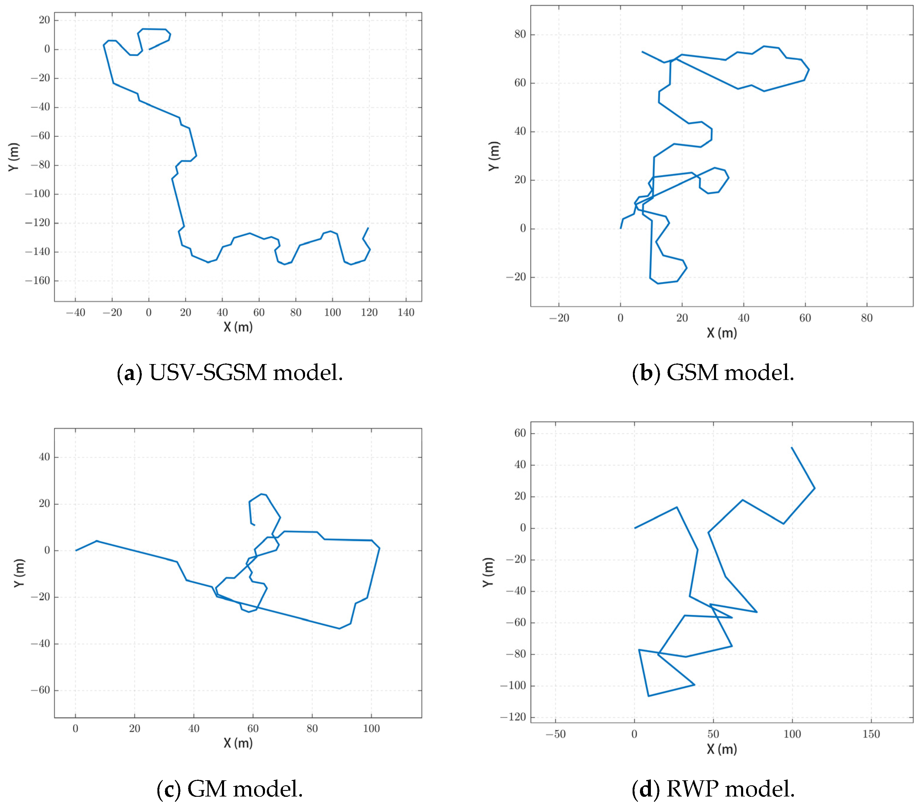
The simulation results of the movement of catamaran USV using the proposed USV-SGSM compared with GSM, GM, and RWP models are shown in
Figure 10. The USV is 7.5 m in length, 2.8 m in width, with a displacement of less than 2.5 tons, and a working sailing speed of 5–12 knots. As can be seen from
Figure 10, in the cyclotronic motion phase, the proposed USV-SGSM model has a suitable steering radius, and its trajectory is smooth, while the steering trajectories of the remaining three models show abrupt changes with obvious inflection points. In the straight-line motion phase (including variable velocity and stable motion phase), the trajectory of the USV-SGSM model shows a slight offset, which is in line with the straight-line motion of the USV under the action of waves, while the trajectories of the remaining three models show a stable straight line. Therefore, the characteristics of the USV-SGSM model are more in line with the real movement characteristics of USV when it is traveling on the sea surface and can more accurately simulate the motion state of the USV, thus laying the foundation for the subsequent simulation of the relevant network performance.
To further quantify the performance of different mobility models,
Table 1 presents two key metrics: steering radius and average link hold time. In vessel design, specific requirements are set for the steering radius to ensure maneuverability. For a USV with good maneuverability, the minimum steering radius is typically around 1.5 m. As shown in
Table 1, the USV-SGSM model exhibits superior cyclotronic characteristics compared to other models and achieves the highest link duration. These results highlight the advantages of the proposed USV-SGSM mobility model.
4.2. Vessel Trajectory Prediction Experiments
The experimental environment for vessel trajectory prediction is configured with CPU: Intel Core i5-11260H 2.60 GHz; RAM: 16.0 GB; and MATLAB R2024b. In this paper, the data set is divided into training, validation, and test sets in the ratio of 8:1:1, where the training set is used for model parameter optimization and feature learning to improve the model’s generalization ability. The validation set assumes the functions of model performance evaluation and structural adjustment and optimizes the hyper-parameters by monitoring the performance on the validation set; the test set, as an independent evaluation set, is used only after the completion of model training and tuning and is used to objectively evaluate the final prediction performance of the model to ensure the fairness and availability of the evaluation results.
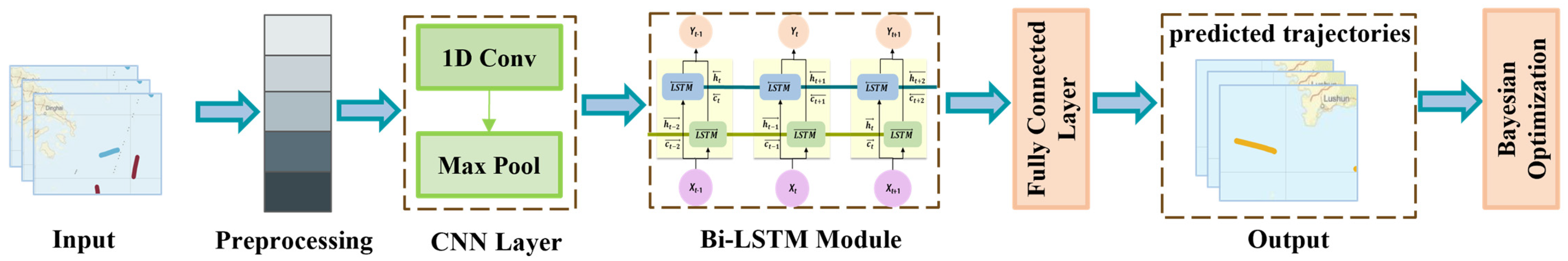
In the trajectory prediction model, the latitude and longitude of the vessel at the next moment are output by inputting the vessel data at four consecutive moments. In the CNN-Bi-LSTM model, the convolution kernel size of 1DCNN is 3, and the output time step is 2. In this paper, we adopt a zero-pooling strategy for the convolution operation, which ensures that the size of the feature map before and after the convolution is consistent by replenishing zero-valued elements at the boundary of the input feature map. Meanwhile, the pooling operation adopts the mean pooling method, i.e., the arithmetic mean of the feature values within the specified sensory field is calculated as the output. This processing not only maintains the spatial dimension of the feature map but also realizes the down sampling of the features, which is conducive to the network to extract more representative feature information. The number of neurons in the forward-backward LSTM layer of the Bi-LSTM is 100, and the number of neurons in the full-connectivity layer is 80, 40, and 10, respectively.
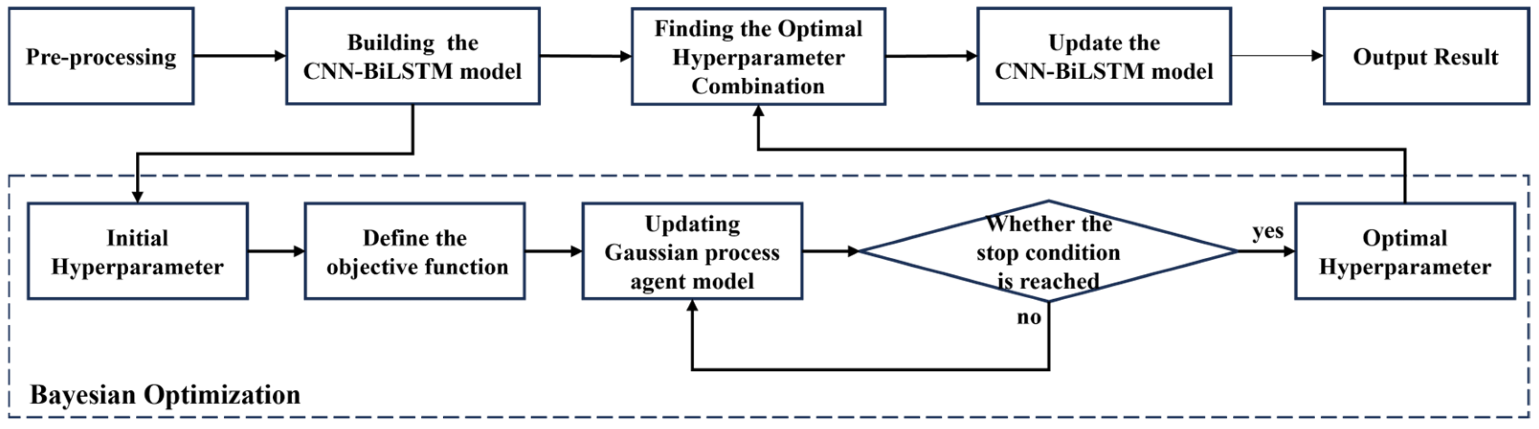
To optimize the hyperparameters of CNN-BiLSTM, we adopt Bayesian optimization, whose time complexity mainly comes from Gaussian process regression and the maximization of the acquisition function. The total complexity of Bayesian optimization is . The time complexity of the CNN part is . The complexity of the Bi-LSTM part is , which dominates the overall computational cost of the model. Future work can further reduce h through pruning to optimize efficiency.
During the optimization of the model in the training and validation sets, the hyper-parameter combinations were tuned using Bayesian optimization, and the specific comparison results are shown in
Table 2.
Comparison of the predicted trajectories obtained by BO-CNN-BiLSTM and real vessel trajectories are shown in
Figure 11, and it can be visualized that the real trajectory of the vessel almost completely overlaps with the predicted trajectory.
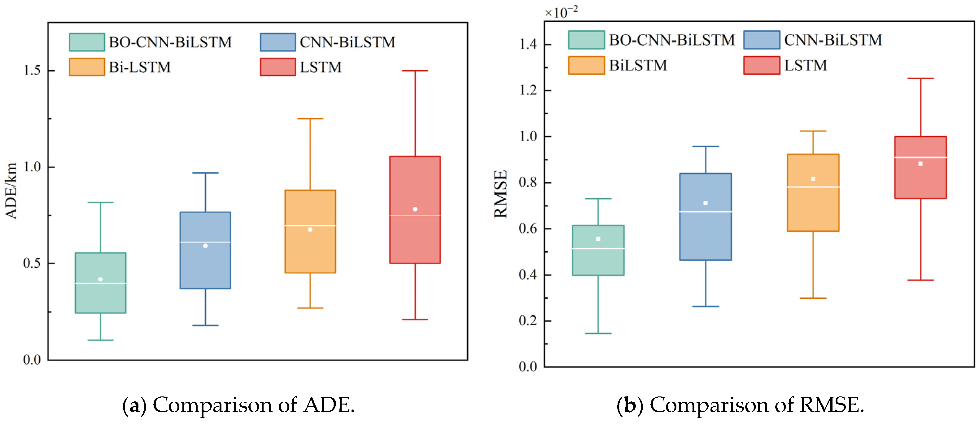
Furthermore, the performance of the BO-CNN-BiLSTM model is evaluated against the CNN-BiLSTM model, the Bi-LSTM model, and the LSTM model [
37], as shown in
Table 3,
Figure 12a,b. The BO-CNN-BiLSTM model shows significant improvements in all three metrics compared to the CNN-BiLSTM algorithm, where the RMSE, Maxerr, and ADE are reduced by 20.77%, 50.36%, and 29.37%. This demonstrates that it can fully utilize the trajectory information extracted from historical trajectories, it has lower performance variance, and effectively improves the trajectory prediction model performance in terms of accuracy and computational efficiency. Moreover, when handling long-term forecasting tasks, it is able to maintain excellent performance.
It can be seen that the proposed BO-CNN-BiLSTM algorithm performs well in the vessel trajectory prediction task, with the smallest average deviation of the prediction results, a narrower range of data distribution, a low degree of discretization, and fewer outliers, which indicates that the model has a high prediction accuracy and stability, and is able to predict the vessel’s trajectory more accurately.
The ten-fold cross-validation method is used to evaluate the performance of the four models. Through cross-validation, the inherent overfitting risk of a single split can be mitigated. The dataset is divided into 10 parts, 9 parts are used as the training set, and 1 part as the testing set for a total of 10 experiments. The average ten-fold cross-validation accuracy of each model is shown in
Table 4.
It can be seen from the table that the proposed BO-CNN-BiLSTM has the best performance, and its average accuracy is significantly higher than that of other models. CNN-BiLSTM is secondary, indicating that the combination of CNN feature extraction and Bi-LSTM timing modeling is better than that of a single LSTM. Bi-LSTM is better than LSTM, which verifies the effectiveness of bi-directional structure.
4.3. Routing Protocol Simulation
In this section, to evaluate the performance of the proposed protocol, two enhanced AODV protocols, FL-AODV [
38] and EASP-AODV [
39], are selected for comparative experimentation. M-MANETs are constructed using the OMNET++ simulation platform. All the network nodes move in the simulation area according to the USV-SGSM model, and the simulation system model only contains the vessel terminal nodes.
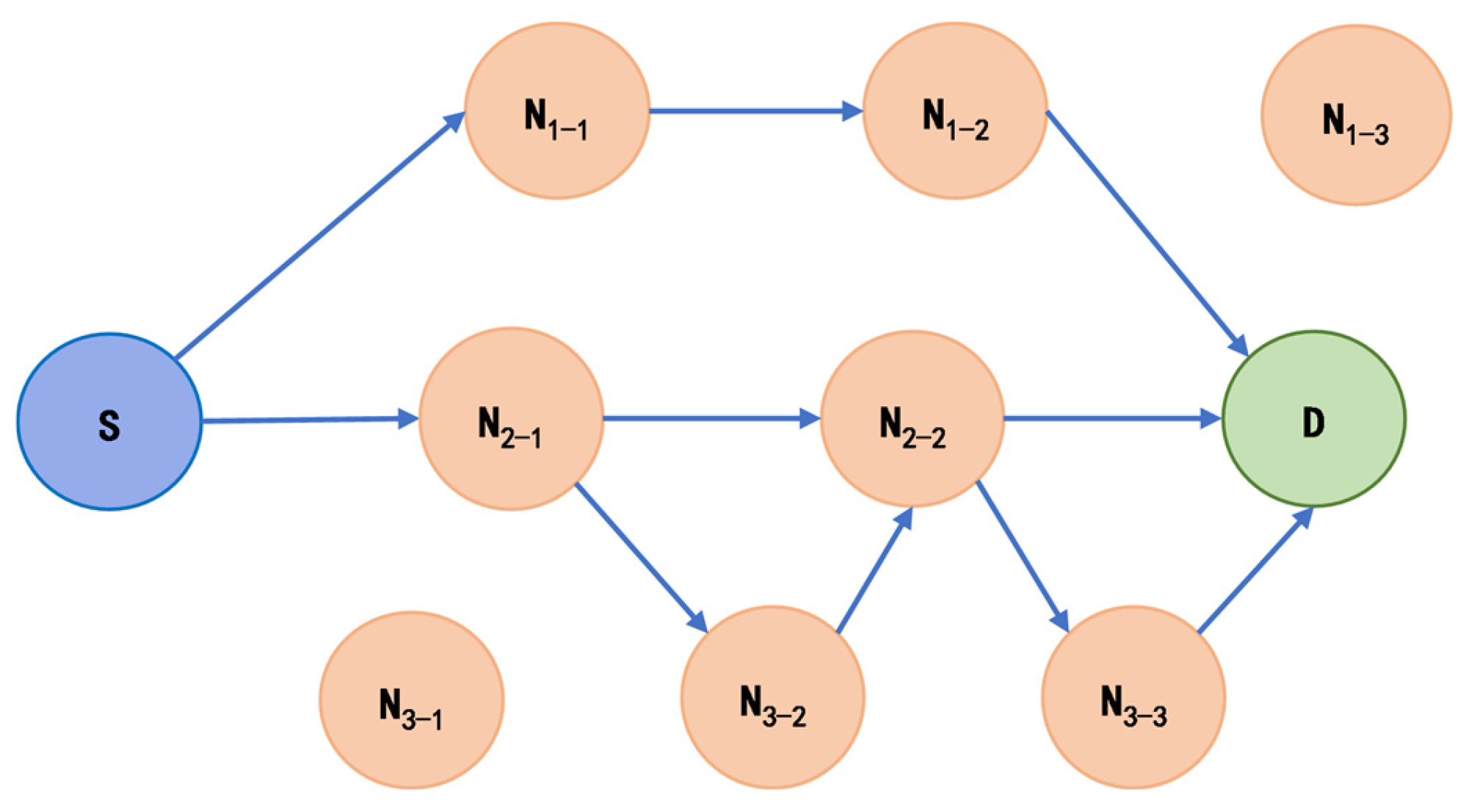
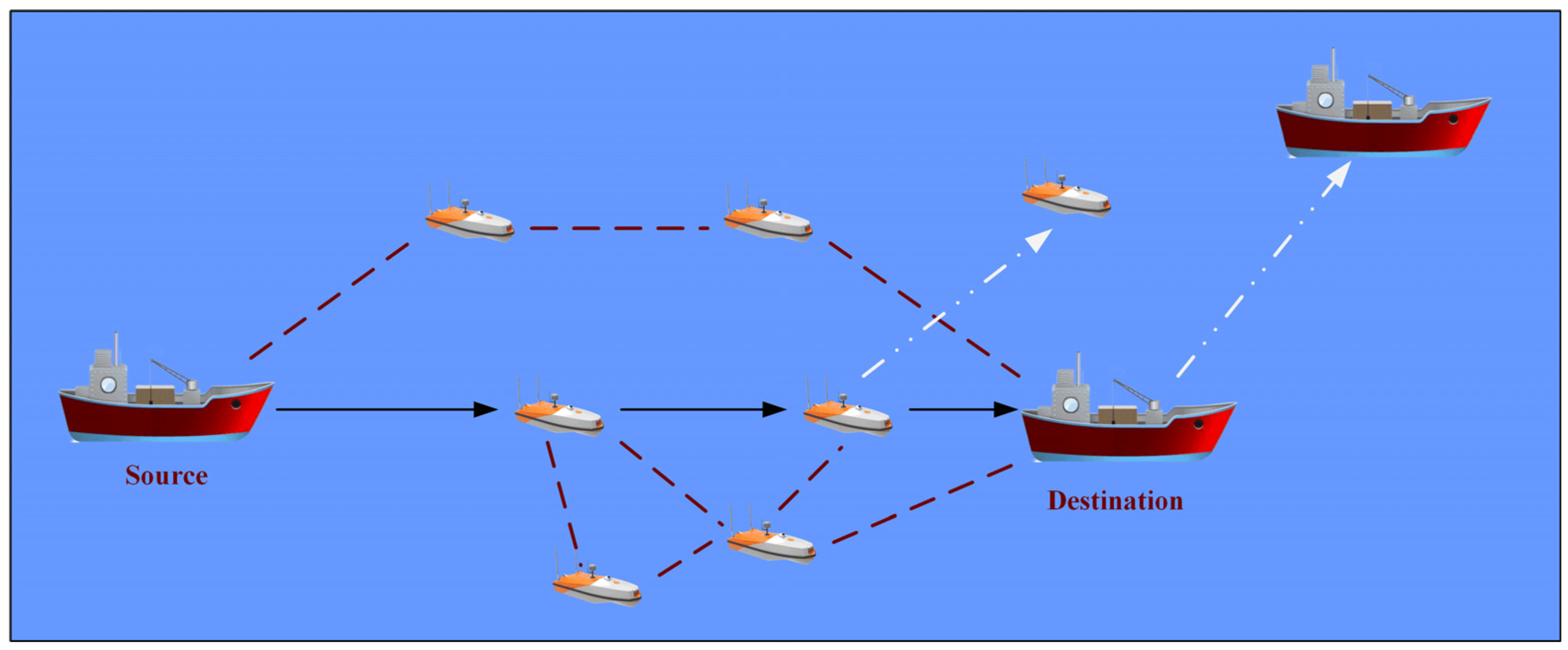
Figure 13 illustrates the M-MANET communication scenario. Multiple potential routing paths exist between the source and destination nodes, depicted by red dashed lines without arrows, while the chosen routing path is indicated by black solid lines with arrows. Taking one USV and the destination node as an example, white dashed lines with arrows are used to represent their directions of movement. In the experiments, USVs are the relay nodes, and the cargo vessels are the source nodes and the destination nodes. Specifically, one cargo vessel acts as the source node, responsible for generating and sending data packets, while another cargo vessel functions as the destination node, receiving the transmitted information. USVs play critical roles in ensuring reliable and efficient communication by relaying signals, particularly in scenarios where direct communication between the source and destination nodes may be hindered by long distances.
Average end-to-end delay, average routing overload, packet delivery rate and network throughput are used to evaluate the performance of routing protocols. For VHF physical layer parameters, we adopted ITU-R M.1842 guidelines for maritime VHF bands. The frequency range is 156–174 MHz, and the propagation models are ITU-R P.1546 for over-water path loss and Rayleigh Fading for small-scale variations.
To ensure the availability of the experimental results, this paper adopts the method of repeating experiments, and each group of simulation experiments is repeated 50 times under the same configuration. Finally, the average value of the results is taken as the final performance evaluation index. The simulation parameters are shown in
Table 5.
Figure 14 shows the detailed data interaction log graph between two vessel nodes of M-MANET intercepted in OMNET++ (OMNet++4.6). As shown in the figure, the cargo vessel node 0 first transmits the data packet to the USV nodes 0, 1, and 2, and after USV node 0 successfully receives the data packet and completes the next-hop node selection, it forwards the data packet to USV node 1. Finally, it is sent through the USV node 1 to complete the transmission of the data packet to the cargo vessel node 1.
This paper focuses on the impact of node movement speed and number of nodes on protocol performance. The node movement speed directly affects the degree of dynamic change of the network topology. When the node movement speed is low, the network topology remains relatively stable, while when the node movement speed is high, the network topology will experience frequent dynamic changes. The maximum speeds of USV nodes are set from 5 m/s to 15 m/s, and the packet sending rate is 10 packets/s.
4.3.1. Average End-to-End Delay Comparison
End-to-end delay refers to the average delay time for all data packets from the source node to the final successful reception of the data by the target node, which can be used to analyze the timeliness of routing. This section evaluates the impact of node mobility and network density on the average end-to-end delay of the three routing protocols.
Figure 15a demonstrates the comparison of the average end-to-end delay performance of the three routing protocols for different node movement speeds. As can be seen from the figure, the average end-to-end delay of all three protocols shows an increasing trend as the node movement speed increases. This is due to the frequent network topology changes and the corresponding increase in routing maintenance overhead. As topology changes accelerate, AODV-LPRI outperforms the other two protocols, reducing average end-to-end latency by 14.59% compared to the FL-AODV protocol.
Figure 15b shows the comparison of the average end-to-end delay performance of the three routing protocols with different numbers of nodes. As can be seen from the figure, with the increase in node density, the average end-to-end delay of the three routing protocols decreases first and then increases. This is due to the small number of nodes and low density, resulting in poor network connectivity and high latency. As the number of nodes increases, the network becomes more connected, and the latency decreases. However, when too many nodes are added, the network size becomes larger; as more relay nodes are selected during path discovery, the average hop count increases dramatically, resulting in a rapid increase in average end-to-end delay. However, AODV-LPRI preferentially selects routes with high link quality to establish links so that the average end-to-end delay of AODV-LPRI is basically lower than that of the other two protocols.
4.3.2. Average Routing Load Comparison
Routing load refers to the ratio of the number of routing control packets sent by all nodes in the network to the number of data packets received by the destination node, which reflects the degree of network congestion. This section studies the routing load of the three protocols under different mobility and network densities and compares the efficiency and routing stability of the three protocols to balance control packets.
Figure 16a shows the comparison of routing load at different node movement speeds. As the topology changes dynamically, the average routing overhead of all three routing protocols keeps increasing. As the speed of node movement increases, the stability of the link decreases, so more control packet packets are required to assist in the transmission of data packets, resulting in an increase in routing overhead. However, the link availability acknowledgment mechanism is added to the AODV-LPRI protocol to increase the number of control packet packets, so the average routing cost of this protocol is higher than that of EASP-AODV. AODV-LPRI outperforms FL-AODV protocol when topology changes are more frequent. This is because AODV-LPRI establishes available routes through link availability, which reduces the frequency of route reconfiguration and has low maintenance costs.
Figure 16b shows the average routing load for the three routing protocols with different node counts. As can be seen, the average routing load of the three routing protocols increases with the increase in node density. Compared with other routing protocols, AODV-LPRI has a lower routing load. The AODV-LPRI routing protocol uses the nodes with high link availability as the next hop nodes to forward packets instead of selecting all neighbor nodes that can communicate for flood forwarding, which reduces the number of intermediate nodes on the communication link and the number of routing control packets is also reduced. Therefore, the AODV-LPRI protocol has a lower routing load than the other two protocols.
4.3.3. Packet Delivery Fraction Comparison
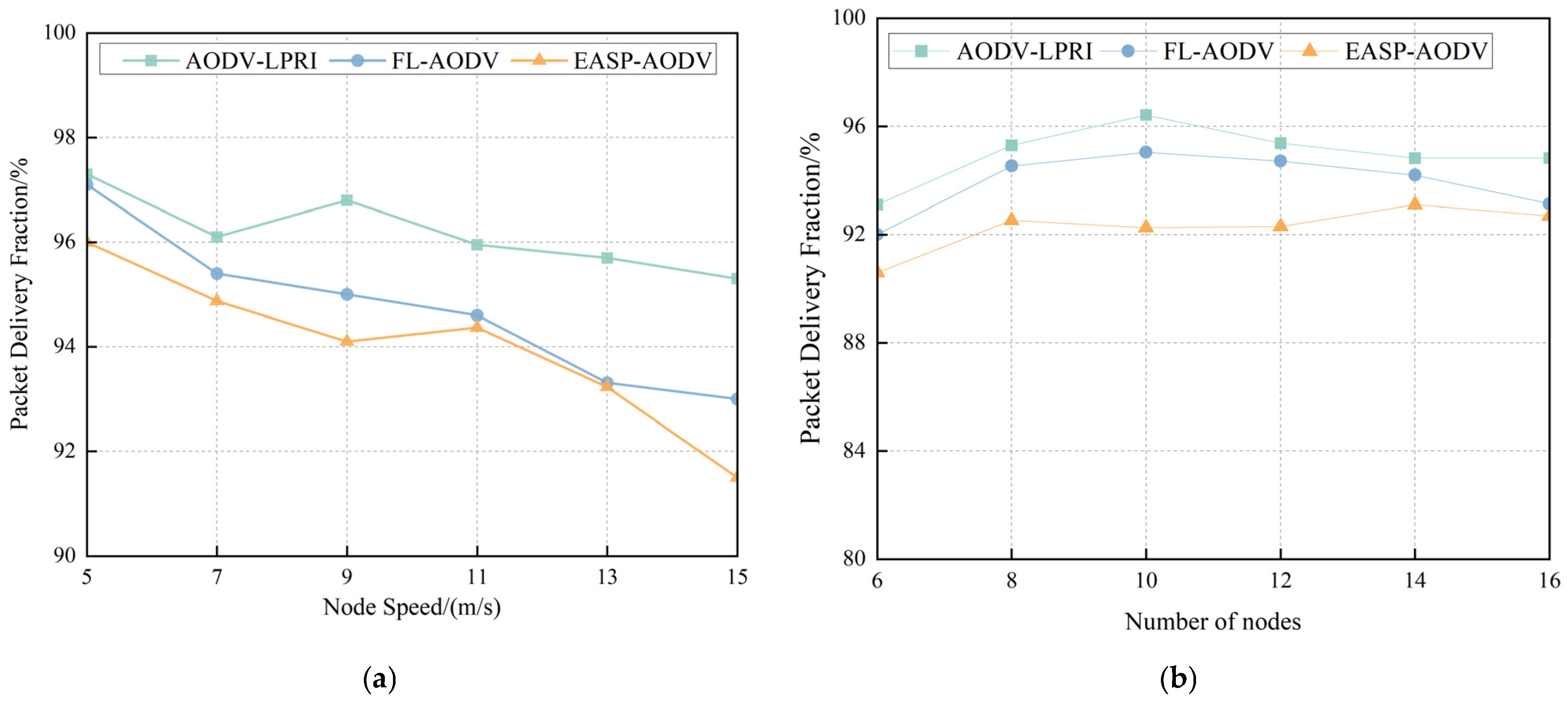
Packet delivery fraction refers to the proportion of packets received over a period of time to the total number of transmissions. The larger the packet delivery fraction, the better the integrity and accuracy of data transmission and the more reliable the network. This section evaluates the reliability of the three routing protocols by analyzing their packet delivery performance at different moving speeds and network densities.
A comparison of the packet delivery fraction performance of the routing protocols under different changes in mobility speed is shown in
Figure 17a. Various routing protocols are gradually decreasing as speeds continue to increase. This is because the stability of the communication link decreases with the increase of the movement speed, which increases the probability of packet loss. AODV-LPRI shows better protocol performance by maintaining a relatively high and stable packet delivery rate over the entire range of node mobility speeds, with an average increase of 1.54% over the packet delivery fraction of the FL-AODV protocol. This is because AODV-LPRI selects routes based on the
routing metric with optimal route availability, which can effectively reduce the packet loss caused by route interruption.
Figure 17b shows the packet delivery fraction performance of the three routing protocols at different node counts. It can be seen from the results that the AODV-LPRI protocol has the best performance in packet delivery fraction and is relatively stable.
In M-MANET, the limitation of the AIS communication rate has a certain impact on the packet delivery fraction of various protocols, but it can be seen from the simulation that the AODV-LPRI protocol has the best performance in packet delivery fraction and is relatively stable, with an average delivery rate of about 94.98%. The more nodes, the more intermediate nodes in the communication link from the source to the destination, and the increase in the number of receiving and forwarding packets, the more congested the network becomes and leads to loss of data packets in transmission. By obtaining the link availability of neighboring nodes, the AODV-LPRI protocol determines whether a node can forward packets. Flood forwarding is restricted, so the packet delivery fraction of the AODV-LPRI routing protocol is higher than that of other routing protocols under the same conditions, especially when the density of nodes is large.
4.3.4. Network Throughput Comparison
Throughput refers to the average number of data packet bits received per unit of time by all target nodes in the network, which is used to analyze the pressure that the network can withstand. This section analyzes the impact of node mobility and network density on throughput.
Figure 18a demonstrates the network throughput performance comparison at different node movement speeds. It can be observed that the network throughput of the three protocols shows a decreasing state as the node movement speed increases. This is because when the topology changes frequently, the link quality decreases, which directly affects the success rate of packet transmission, thus leading to a decrease in network throughput. However, AODV-LPRI outperformed the other two protocols, with an average 4.43% increase in network throughput compared to the FL-AODV protocol. This performance advantage is due to the fact that AODV-LPRI introduces the link availability evaluation mechanism that monitors the link status in real-time and selects available routes based on
routing metric, which effectively reduces the frequency of routing reconfiguration and improves the packet transmission rate and, thus, the AODV-LPRI can maintain a high network throughput.
Figure 18b illustrates the network throughput of the three routing protocols with different numbers of nodes. With the increase in the number of nodes, the number of nodes in the communication range of a node increases, which means that the number of intermediate nodes in the communication link between the source node and the destination node increases, and the nodes in the communication range need to receive and forward data packets, resulting in the network becoming congested, and the number of data packets successfully transmitted per unit time decreases, so the network throughput of these three protocols first increases and then decreases. However, compared with other routing protocols, the AODV-LPRI routing protocol selects the node with high link availability as the next-hop node to forward packets instead of selecting all neighbor nodes that can communicate for forwarding, which reduces the number of next-hop nodes selected and reduces the congestion degree of the network. Therefore, the AODV-LPRI routing protocol has a larger network throughput than other routing protocols.
4.4. Discussion
The simulation experiments in this section systematically validate the effectiveness of the proposed models and routing metrics. In terms of the mobility model, the proposed USV-SGSM model demonstrates superior performance in simulating real-world vessel movements. Compared with traditional models, it achieves a more reasonable steering radius and significantly longer average link hold time, reducing abrupt trajectory changes and better reflecting the smooth motion characteristics of USVs under marine environmental constraints. This improvement enables more accurate simulation of network topology dynamics in M-MANET.
For vessel trajectory prediction, the proposed BO-CNN-BiLSTM model shows remarkable accuracy and stability. It reduces the RMSE by 20.77%, Maxerr by 50.36%, and ADE by 29.37% compared with the CNN-BiLSTM model. The integration of Bayesian optimization enhances the model’s ability to capture spatiotemporal correlations in trajectories, making it more suitable for predicting the motion patterns of large vessels and providing reliable a priori information for link state estimation.
In routing protocol performance, the proposed AODV-LPRI protocol based on link availability achieves comprehensive optimizations. It reduces the average end-to-end delay by 14.59%, increases the packet delivery fraction by 1.54%, and improves network throughput by 4.43% compared with benchmark methods. The routing metric that integrates link availability effectively mitigates the impact of dynamic topology changes, demonstrating strong adaptability in dynamic maritime scenarios.
Collectively, these results confirm that the proposed framework establishes a tight coupling among mobility modeling, trajectory prediction, and routing metrics design, providing a practical solution for enhancing the stability and efficiency of M-MANET.


