A Computational Study on the Excitation Forces of Partially Submerged Propellers for High-Speed Boats

Abstract

During high-speed navigation, boat propellers often become partially exposed due to elevated sailing speeds. This condition results in a unique operational scenario where propellers are only partially submerged. Conducting computational studies on the excitation of propellers under such circumstances is essential for optimizing the dynamic performance of the shafting system. A theoretical calculation method for propeller performance was developed based on the principles of fluid dynamics relevant to water entry, leading to a computational method for determining excitation forces in this specific operational condition. This method was subsequently refined through appropriate adjustments using ANSYS Fluent software to simulate the behavior of partially submerged propellers. The findings highlighted the accuracy of the proposed model in predicting the pulsation of six force components across three distinct directions: along the propeller shaft, vertical, and lateral. Specifically, for a single blade (Blade 1), the pulsation amplitude of the vertical force (Fx) constituted 82.1% of its maximum peak magnitude and equated to 57.5% of the blade’s mean thrust. Analogously, the lateral force (Fz) pulsation amplitude represented 53.3% of its maximum peak magnitude and 40.0% of the mean thrust. These findings indicate the presence of significant unsteady hydrodynamic loads. Furthermore, a visualization approach was presented to analyze blade load phasing, offering insights relevant to the arrangement of blades on partially submerged propellers.

1. Introduction

Partially submerged propellers, also called semi-submerged water propellers or surface propellers, are a specialized type of propeller that operates efficiently when a vessel is navigating at high speeds, specifically at its designed speed. These propellers generate open water areas around the propeller shaft as the blades are cyclically immersed in and emerge from the water. Such design facilitates enhanced efficiency and reduces appendage resistance in high-speed vessels, making them suitable for application in high-speed boats and shallow-draft craft.

A partially submerged propeller differs from standard propellers in that it has some blades operating in air and some in water, resulting in an asymmetric force distribution throughout the entire propeller. This asymmetry further results in periodic variations in six force components (three force components and three moment components) in three directions. A large lateral force can greatly influence the dynamic loading and stability of the boat’s shaft and the longitudinal motion status of the vessel.

Reduced submergence depth mitigates blade cavitation risk but amplifies thrust/torque pulsations. Experimental data indicate that thrust fluctuation amplitudes increase by 200–300% in comparison with steady-state conditions at immersion ratios (h/R) < 0.3. Within advance coefficients of 0.8–1.4, partially submerged propellers achieve peak thrust coefficients and propulsion efficiency, albeit with pronounced periodic fluctuations in lateral/vertical forces [1,2,3]. These instabilities originate from gas–liquid interface dynamics during blade water-entry/exit events. Under naturally ventilated conditions, spiral-shaped air cavities form on the suction side of the blade, which can reduce the torque requirement but increase the turbulence energy level of the flow field. Conversely, forced ventilation effectively optimizes the load distribution on the blade surface through precise control of the gas–liquid mixture ratio via ventilation tubes, reducing the amplitude of thrust fluctuation by about 40% [4].

Additionally, whirling vibration primarily originates from periodic lateral forces from the propeller, oil film instability in bearings, or mass eccentricity of the shaft system, while lateral vibration is often dominated by unbalanced mass or external impact loads [5,6,7,8]. Understanding the nature and magnitude of these propeller-induced excitation forces, especially the lateral components, is therefore crucial for predicting and mitigating potential shafting vibrations in high-speed boats employing partially submerged propellers.

Worldwide, studies examining the performance of forces on partially submerged propellers primarily utilize two approaches: theoretical computation and hydrodynamic experiment. When establishing a computational model, the theoretical computation method relies on several assumptions, which could potentially lead to some variance from the actual circumstances [9,10]. Vorus [11] expanded Lewis’s [12] traditional propeller theory to determine the stable forces and moments on partially submerged propellers. This approach assumes a linear relationship between the steady sectional lift coefficient ($\nabla C_L$) and the incremental blade sectional attack angle ($\nabla \alpha$), akin to a fully ventilated flat plate (starting from the leading edge of the plate).

$$\nabla C_L={\displaystyle \frac{\pi }{4}}\nabla \alpha$$

(1)

The model incorporates blade pitch angle, skew, and rake geometry, serving as a user-friendly design tool for comparative studies and blade shape optimization [11]. However, its oversimplified assumptions preclude accurate predictions of dynamic blade loads.

Kudo and Ukon [13] and Kudo and Kinnas [14] extended the three-dimensional lifting-surface vortex lattice method to analyze super-cavitating propellers in addition to partially submerged propellers. Nevertheless, this technique assumes full propeller immersion during calculations. The resultant stabilizing forces and moments are subsequently multiplied by the propeller’s submergence ratio. Consequently, only estimates of average forces are acquired, overlooking the complex phenomenon of blades slicing through the water’s surface as they emerge and submerge. Savineau and Kinnas [15] developed a 2D time-marching boundary element method to analyze the fluid dynamics surrounding completely aerated and partially sunken hydrofoils. This method also supposes that the ventilated cavity is separated from the front edge of the blade. However, this method solely considers a situation whereby the hydrofoil enters the water, disregarding the scenario where the hydrofoil gets away from the water. Moreover, this method neglects the influences of water jets and free surface elevation variations due to the implementation of a negative image method.

In a study conducted by Rose [16], five Rolla-type propeller models with four blades were examined under partial submergence. The research involved gathering time-averaged experimental data on thrust, torque, and vertical/lateral forces at varying submergence ratios, shafting inclination angles, and cavitation numbers. As a result of this study, a series of design charts were created specifically for partially submerged propellers operating at 35–45 knots. Olofsson [17] conducted a study where separated propeller blades were installed on a force-measuring propeller hub to individually measure the forces acting on each blade. This research focused on analyzing how cavitation number and Froude number impacted the properties of partially submerged propellers. For more in-depth information on this study, Olofsson’s doctoral thesis [18] serves as a comprehensive resource. While experimental studies have provided a foundational understanding of partially submerged propellers and led to numerous overarching conclusions, these studies predominantly highlight general force characteristics, often lacking precise details about the flow field dynamics. Miller and Szantyr [19] investigated the thrust, torque, and lateral forces of partially submerged propellers at various submergence ratios, shafting inclination angles, and lateral angles. Furthermore, they analyzed the experimental results to determine the unstable bending moments on single blades.

Numerical simulation enables comprehensive predictions to be made of propeller forces and full-flow-field analysis. Although computational fluid dynamics (CFD) applies to partially submerged propellers, their complex free-surface interactions introduce significant computational challenges, explaining the limited CFD literature. In a study conducted by Caponnetto [20], the Comet software, employing the Finite Volume Method (FVM) combined with the Reynolds-Averaged Navier–Stokes (RANS) approach, was utilized to conduct numerical simulations for partially submerged propellers. The findings of this study indicated that the thrust variations over one revolution cycle of a blade closely matched the experimental values. However, this study did not include the performance curves of partially submerged propellers.

Rooted in the principles of fluid dynamics governing water entry, this study first considered the theoretical basis of propeller performance to gain insights into the excitation forces under partially submerged operating conditions. To facilitate a comprehensive analysis, numerical simulations of a three-blade, right-hand partially submerged propeller were subsequently performed using the Ansys Fluent CFD software 2021 R1. This computational investigation, which employed the RANS method, the VOF method for free-surface tracking, and a sliding mesh technique for simulating rotation, thoroughly examined the periodic characteristics of the excitation forces and revealed their unique variations under such challenging conditions.

2. Computation Method

The analytic formulas for propellers that are partially submerged are comparable to those used for fully submerged propellers. Kinnas and Fine [21], Young and Kinnas (2001) [22], and Young and Kinnas (2003c) [23] introduced these formulas. For completeness, an overview is provided here. As shown in Figure 1, we consider a partially submerged propeller affected by a general inflow wake, denoted as ${\overrightarrow{q}}_w(x,y,z)$. The inflow wake is represented by an absolute coordinate system (X, Y, Z) (fixed coordinate system of the boat), and is regarded as an effective wake (i.e., including the interactive action between the vorticity of inflow and the propeller [24,25]). The inflow velocity ${\overrightarrow{q}}_{in}$ relative to the fixed coordinate system of the boat (X, Y, Z) is defined as the sum of the inflowing wake velocity ${\overrightarrow{q}}_w$ and the propeller’s angular velocity $\omega$. At a given position $\overrightarrow{x}$, the following equation holds:

$${\overrightarrow{q}}_{in}\left(x,y,z,t\right)={\overrightarrow{q}}_w\left(x,r,{\theta }_B-\omega t\right)+\overrightarrow{\omega }\times \overrightarrow{x}$$

(2)

where $r=\sqrt{y^2+z^2}$, ${\theta }_B=\mathrm{a}\mathrm{r}\mathrm{c}\mathrm{t}\mathrm{a}\mathrm{n}(z/y)$, and $\overrightarrow{x}=(x,y,z)$. It is assumed that the resulting flow is both non-compressible and inviscid. Therefore, the total velocity $\overrightarrow{q}$ can be represented using ${\overrightarrow{q}}_{in}$ and the perturbation potential $\varphi$:

$$\overrightarrow{q}\left(x,y,z,t\right)={\overrightarrow{q}}_{in}\left(x,y,z,t\right)+\overrightarrow{\nabla }\varphi (x,y,z,t)$$

(3)

where $\varphi$ obeys Laplace’s equation within the fluid region (i.e., ${\nabla }^2\varphi$ = 0). The fixed coordinate system of the boat is used for the flow analysis.

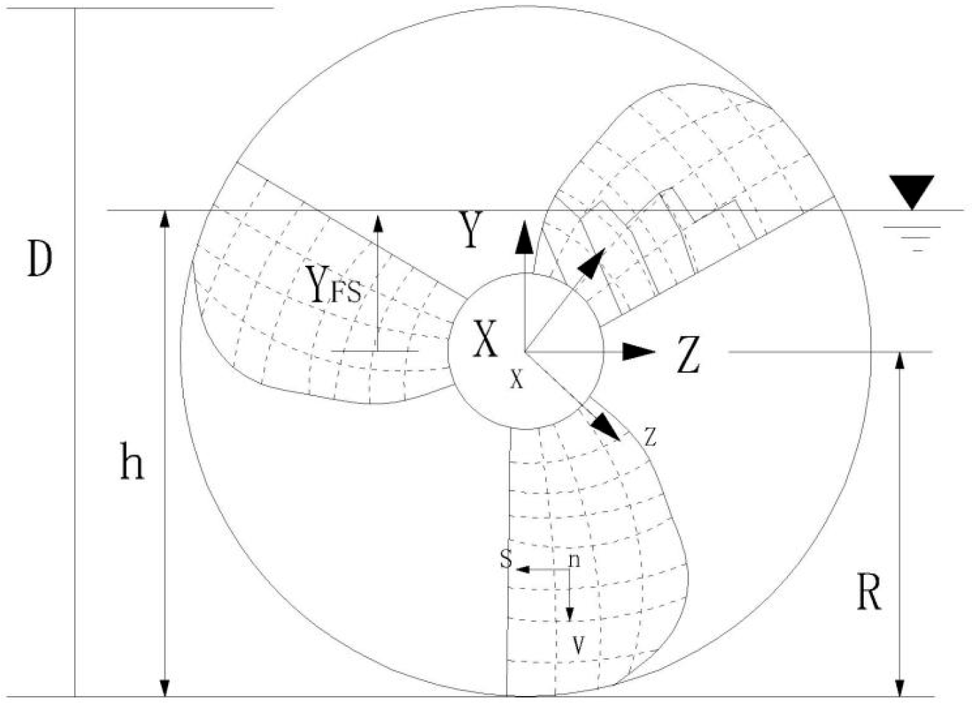
2.1. Linearized Boundary Conditions for Free Surfaces

The current numerical model employs linearized boundary conditions to clarify the impact of free surfaces. The governing equation is expressed as follows:

$${\displaystyle \frac{{\partial }^2\varphi }{{\partial t}^2}}\left(x,y,z,t\right)+g{\displaystyle \frac{\partial \varphi }{\partial Y}}\left(x,y,z,t\right)=0 \mathrm{at} Y=-R+h (i.e. free surface)$$

(4)

where h and R, respectively, represent the submerged depth of the blade tip and the radius of the blade, as defined in Figure 2. Y denotes the fixed longitudinal coordinate of the boat, as defined in Figure 2.

Assuming that the criteria for an infinitely large Froude number are satisfied:

$$\left(i.e., F_{nD}={\displaystyle \frac{V}{\sqrt{gd}}}\to \mathrm{\infty }\right),$$

(5)

Equation (4) can be simplified to:

$$\varphi (x,y,z,t)=0\mathrm{at} Y=-R+h$$

(6)

Given that partially submerged propellers typically function at extremely high speeds, it is reasonable to assume that there is no limit to the growth in the Froude number. Research conducted by Shiba [26], Brandt [27], and Olofsson [18] has demonstrated that, in situations when there is sufficient ventilation, the significance of the Froude number becomes negligible when $F_{nD}$ > 4.

It is important to note that this assumption of an infinite Froude number (and the resulting simplification in Equation (6)) is specific to the theoretical boundary-integral formulation presented in Section 2. The primary CFD simulations detailed from Section 3 onwards inherently account for gravitational effects and finite Froude number conditions through the inclusion of gravity in the momentum equations and the Volume of Fluid (VOF) method for free surface capturing.

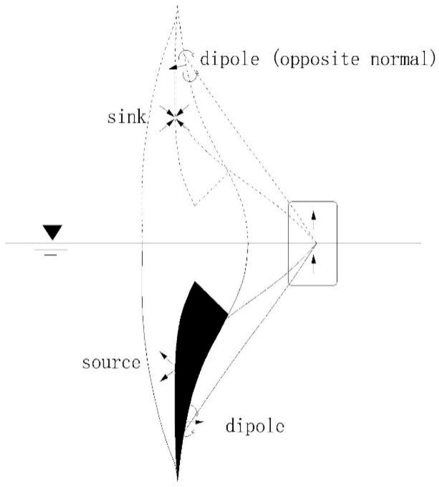
2.2. Boundary Integral Equation

The relationship described in Equation (6) underscores the relevance of the negative image concept in elucidating the impact of free surfaces. Hence, the perturbation potential $\varphi$ at each point p on the submerged part of the surfaces of submerged blades and ventilated cavities can be expressed as follows:

$${\varphi }_P={{\phi }_P}^S+{{\phi }_p}^i$$

(7)

where ${{\phi }_p}^s$ denotes the potential generated at point p under the influence of sources and dipoles associated with submerged blades and ventilated cavities:

$${{2\pi \varphi }_p}^s(t)=\iint S(t)\left[{\varphi }_q(t){\displaystyle \frac{\partial G\left(p;q\right)}{{\partial n}_q\left(t\right)}}-G(p;q){\displaystyle \frac{{\partial \varphi }_q(t)}{{\partial n}_q(t)}}\right]dS$$

(8)

${{\phi }_p}^{i }$ denotes the potential arises at point p as a result of the dipoles and sources that mimic the images of submerged blades and ventilated cavities.

$${{2\pi \varphi }_p}^i\left(t\right)=-\iint S(t)\left[{\varphi }_q(t){\displaystyle \frac{\partial G\left(p;\widehat{q}\right)}{{\partial n}_{\widehat{q}}\left(t\right)}}-G(p;\widehat{q}){\displaystyle \frac{{\partial \varphi }_q(t)}{{\partial n}_{\widehat{q}}(t)}}\right]dS$$

(9)

As exhibited in Figure 3, S(t) denotes the dynamic integral surface consisting of the segments parts of the wetted blade surface S_WB(t) and the ventilated cavity surface S_C(t) = S_C1(t) $\cup$ S_C2(t) $\cup$ S_C3(t); G(p; q) = 1/R(p; q) serves as a Green’s function; R(p; q) denotes the distance between points p and q. ${\overrightarrow{n}}_q$ represents the unit vector on the integral surface perpendicular to element q and positively directed toward the fluid domain; variables q and $\widehat{q}$ represent the integral points on the real integral surface and the image integral surface, respectively. The negative sign in front of the integral in Equation (9) reflects the balance between the real singularity and the image singularity, as seen in Figure 4.

Equations (8) and (9) are intended to apply to the “exact” ventilated cavity surface, S_C(t). Nevertheless, rather than being pre-determined, the surface of the ventilation cavity must be validated as part of the overall solution. In this study, a rough ventilated cavity surface was utilized. It consisted of the blade surface below the ventilated cavity S_C2(t) → S_CB(t) and the wake surface portion overlapping with the ventilated cavity S_C1(t) $\cup$ S_C3(t) → S_CW(t). S_CB(t) and S_CW(t) are defined in Figure 3. The studies by Kinnas and Fine [28] and Fine [29] provide information on the measurement of the reasoning underlying this estimate, as well as its impact on the behavior of submerged propeller cavities.

2.3. Moving Boundary Conditions for Wetted Blade Surfaces

When dealing with moving boundary conditions, it is crucial for the water flow to remain aligned with the surface of the wetted blades. This leads to the establishment of a Neumann-type boundary condition for ${\displaystyle \frac{\partial \varphi }{\partial n}}$:

$${\displaystyle \frac{\partial \varphi }{\partial n}}=-{\overrightarrow{q}}_{in}·\overrightarrow{n}$$

(10)

2.4. Dynamic Boundary Conditions for a Ventilated Cavity Surface

Dynamic boundary conditions require that the pressures at all points on the surface of the ventilated cavity remain unchanged and equivalent to the atmospheric pressure P_atm. Utilizing the Bernoulli equation, the total velocity ${\overrightarrow{q}}_c$ at the surface of the ventilated cavity can be formulated as below:

$${\left|{\overrightarrow{q}}_c\right|}^2=n^2{D}^2{\sigma }_n{+\left|{\overrightarrow{q}}_w\right|}^2+{\omega }^2{r}^2-2gY-2{\displaystyle \frac{\partial \varphi }{\partial t}}$$

(11)

where ${\sigma }_n\equiv (Po-Pc)/O-s\rho n^2{D}^2$) is the cavitation number under a ventilation condition; $\rho$ is the fluid density; r is the distance from the rotation axis; P_o is the upstream water-surface static pressure; P_c is the cavity pressure; g is the gravitational acceleration; Y is the fixed longitudinal coordinate of the boat (Figure 2); $n=\omega /2\pi$ and D refer to the propeller’s rotational speed and diameter, respectively.

The present formulation for a partially submerged propeller assumes that the cavity is filled with air and is exposed to atmospheric conditions. Therefore, P_c = P_o = P_atm (atmospheric pressure) and ${\sigma }_n$ = 0. This allows for the omission of the first term on the right-hand side of Equation (11). However, it is important to retain the first term for future modeling of cavitation and partially ventilated flow states in cavities filled with steam and gas.

The overall velocity in the ventilated cavity can be represented by using local derivatives along the s (chordwise), v (spanwise), and n (normal) mesh directions, as displayed in Figure 2.

$${\overrightarrow{q}}_c={\displaystyle \frac{V_s\left[\overrightarrow{s}-(\overrightarrow{s}·\overrightarrow{v})\overrightarrow{v}\right]+V_v\left[\overrightarrow{v}-(\overrightarrow{s}·\overrightarrow{v})\overrightarrow{s}\right]}{{‖\overrightarrow{s}\times \overrightarrow{v}‖}^2}}=\left(V_n\right)\overrightarrow{n}$$

(12)

where $\overrightarrow{s}$, $\overrightarrow{v}$, and $\overrightarrow{n}$ represent unit vectors along the non-orthogonal curvilinear coordinates s, v, and n, respectively. The total velocity ($V_s$, $V_v$, $V_n$) at a local coordinate is defined as follows:

$$V_s\equiv {\displaystyle \frac{\partial \varphi }{\partial s}}+{\overrightarrow{q}}_{in}·\overrightarrow{s}; V_v\equiv {\displaystyle \frac{\partial \varphi }{\partial v}}+{\overrightarrow{q}}_{in}·\overrightarrow{v}; V_n\equiv {\displaystyle \frac{\partial \varphi }{\partial n}}+{\overrightarrow{q}}_{in}·\overrightarrow{n}$$

(13)

The overall normal velocity $V_n$ would be 0 if s, v, and n lie on the “exact” ventilated cavity surface. However, this assumption does not hold because the ventilated cavity surface approximates the wake surface overlapping with the cavity on the blade surface beneath it. While $V_n$ may not precisely equal zero on the approximated cavity surface, it is small enough to be negligible under dynamic boundary conditions [29].

Integrating Equations (11) and (12) yielded a quadratic equation for $\partial \varphi /\partial s$, expressed in terms of the unknown chordwise perturbation velocity. Then, the root that corresponds to the cavity position vector pointing downstream was selected, resulting in the following expression:

$${\displaystyle \frac{\partial \varphi }{\partial s}}=-{\overrightarrow{q}}_{in}·\overrightarrow{s}+V_v\cos \psi +\sin \psi \sqrt{{\left|{\overrightarrow{q}}_C\right|}^2-{V_v}^2}$$

(14)

where $\psi$ represents the angle between the s and v directions (Figure 3). Subsequently, Equation (14) was integrated, forming the Dirichlet-type boundary conditions for $\varphi$. In Equation (14), the terms $\partial \varphi /\partial t$ and $\partial \varphi /\partial \upsilon$ within $\left|{\overrightarrow{q}}_c\right|$ and V_v remain unknown and need to be determined iteratively.

2.5. Moving Boundary Conditions for a Ventilated Cavitation Surface

Under moving boundary conditions, the total velocity perpendicular to the surface of the ventilated cavity must be zero. The governing equation can be expressed as:

$${\displaystyle \frac{D}{Dt}}\left(n-h\left(s,v,t\right)\right)=\left[{\displaystyle \frac{\partial }{\partial t}}+{\overrightarrow{q}}_c\left(x,y,z,t\right)·\overrightarrow{\nabla }\right]\times \left(n-h\left(s,v,t\right)\right)=0$$

(15)

where n and h are, respectively, the curvilinear coordinates perpendicular to the blade surface and the cavity thickness.

Substituting Equation (12) into Equation (15), we obtained the partial differential equation for h on a blade [21]:

$${\displaystyle \frac{\partial h}{\partial s}}\left[V_s-\cos \psi V_v\right]+{\displaystyle \frac{\partial h}{\partial v}}\times \left[V_v-\cos \psi V_s\right]={\sin }^2\psi \left(V_n-{\displaystyle \frac{\partial h}{\partial t}}\right)$$

(16)

This method also further assumes that the cross-flow velocity along the blade surface is negligible (i.e., V_v ≈ V_s cos$\psi$ on S_CB(t)). As such, the term $\partial h/\partial \upsilon$ in Equation (16) becomes zero. Fine [29] conducted a study that substantiated the validity of this assumption, demonstrating that the cross-flow terms computed through iterative processes exerted minimal influence on the projected super-cavities of three-dimensional hydrofoils and propeller blades. Furthermore, partially submerged propellers can hardly be assessed using the term $\partial h/\partial \upsilon$ due to the interference of free surfaces with the ventilated cavity. However, this method faces difficulties in accurately predicting the load on the blade during its entry and exit stages. Furthermore, it is incapable of accounting for the effects of blade vibration, particularly at high speeds.

3. Numerical Simulation

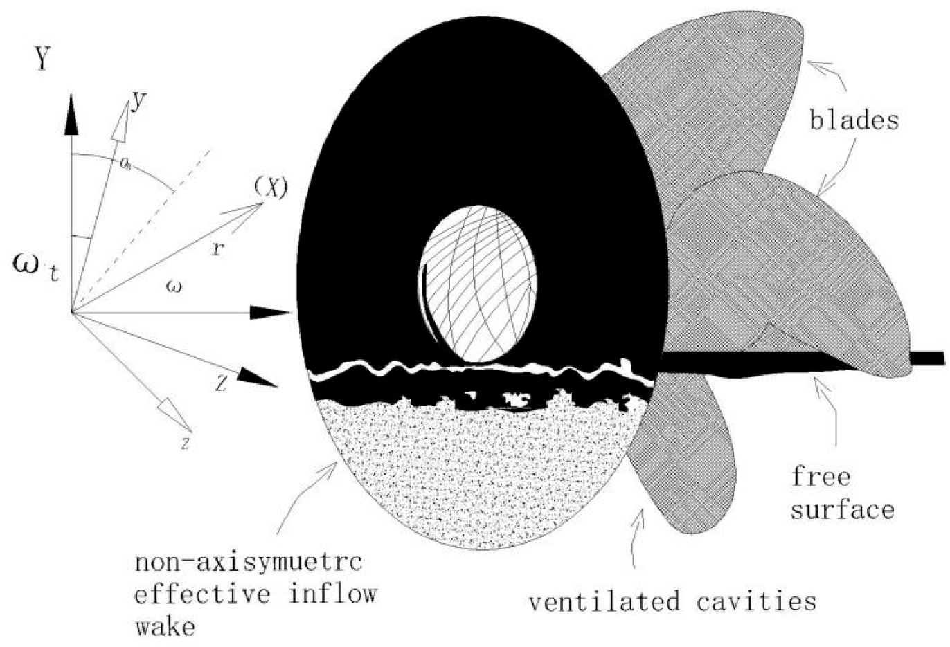
3.1. Fluid Domain Modeling

The numerical simulation employed a partially submerged right-handed three-blade propeller (radius: 600 mm, mean pitch ratio: 1.46, and blade submergence ratio I: 0.5). In this configuration, the lower section of the propeller was immersed in water. The blade profile was designed with a crescent shape and a concave edge, showcasing the distinctive features typical of partially submerged propellers. The dimensions of the fluid domain selected for this simulation were 1800 mm by 1500 mm by 1500 mm. Figure 5 presents the layout of the fluid domain and its spatial coordinates. In the diagram, the lower part represents water, while the upper part represents air. The operational parameters of the partially submerged propeller were assessed by establishing inflow conditions at the fluid inlet and outlet. In this study, the direction along which the water flows is the positive y-axis, with the propeller shaft direction designated as the negative y-axis. The positive x-axis is oriented parallel to the upward direction along the propeller shaft, and the positive z-axis extends outward along the propeller shaft. The excitation force in the x-direction is comprised of both the vertical force and the lateral moment. In the y-direction, the excitation force includes the thrust and the torque. Furthermore, the excitation force in the z-direction is characterized by the lateral force and the vertical moment.

3.2. Governing Equations

The flow characteristics surrounding the partially submerged propeller can be delineated by a comprehensive set of equations reflecting a three-dimensional, time-varying, dual-phase flow regime, portraying air and water as non-compressible mediums. Furthermore, the analysis did not consider the energy exchange between these two states and the phenomenon of surface tension. The governing equations are specified as follows:

Continuity equation (for unsteady, incompressible flow where $\partial \rho /\partial t=0$):

$${\displaystyle \frac{\partial }{\partial x_i}}\left(\rho u_i\right)=0$$

(17)

Momentum equation:

$${\displaystyle \frac{\partial }{\partial t}}\left(\rho u_i\right)+{\displaystyle \frac{\partial }{\partial x_j}}\left(\rho u_i{u}_j\right)=-{\displaystyle \frac{\partial p}{\partial x_i}}+{\displaystyle \frac{\partial }{\partial x_j}}\left(\mu {\displaystyle \frac{\partial u_i}{\partial x_j}}-\rho \overline{u_i^{\prime }{u}_j^{\prime }}\right)$$

(18)

where $u$ is the time-averaged velocity; $u^{\prime }$ is the pulsation velocity; $-\rho \overline{u_i^{\prime }{u}_j^{\prime }}$ is the Reynolds stress; $p$ is the time-averaged pressure; $\rho$ is the mixed density of water and air; $\mu$ is the mixed dynamic viscosity coefficient.

The formulas for their calculations are provided below:

$$\rho =F_w{\rho }_w+F_a{\rho }_a$$

(19)

$$\mu =F_w{\mu }_w+F_a{\mu }_a$$

(20)

$$F_w+F_a=1$$

(21)

where $F$ represents the volume fraction; $a$ and $w$ represent air and water, respectively.

Currently, numerous techniques have been developed for capturing free liquid surfaces, among which the Volume of Fluid (VOF) method was employed in this investigation. This technique is adept at handling complex nonlinear flows and has found extensive application in the field of computational fluid dynamics (CFD). Moreover, it is characterized by its straightforward implementation, high efficiency, minimal computational demands, and low memory consumption. The fundamental principle underlying this technique involves determining the geometry of a free surface through the calculation of the volume fraction function F, which represents the ratio of the fluid volume to the total volume of the computational mesh, without regard to the motion of particles at free liquid surfaces. In our analysis, we focused on computing the volume fraction F. The transport equation governing this process is given by:

$${\displaystyle \frac{\partial F_w}{\partial t}}+\overrightarrow{V}·\nabla F_w=0$$

(22)

If $F_w$ is 0, it signifies that the mesh is entirely filled with air; if $F_w$ is 1, it indicates full saturation with water; if $F_w$ is valued between 0 and 1, it signifies that the mesh is at the water–air interface.

In the computational analysis of the flow field, the viscosity of the fluid was taken into account. The RNG k-ε model, recognized for its suitability in analyzing rotating machinery, was employed to simulate the turbulent behavior of the fluid. This model, introduced by Yakhot and Orzag in 1986 [30], is also known as the Renormalization Group k-ε Model. Structurally, it resembles the conventional k-ε model; however, it adds an extra term to the ε equation, thereby enhancing the simulation accuracy for flows featuring high speeds. The RNG model features modifications to the turbulent dynamic viscosity coefficient, which allows for the consideration of the effects of mean flow rotation and rotational flow states. Consequently, it facilitates more precise predictions concerning the impacts of transient flows and the behavior of curved streamlines. Furthermore, the model accounts for the influence of vortices on turbulence, which improves precision in forecasting conditions associated with swirling flows.

To attain a high level of computational precision, the terms for convection were calculated with a second-order upwind differencing scheme; those for diffusion were computed utilizing a second-order central differencing scheme; the transient terms were calculated via the usage of a first-order implicit scheme. During the solution of the equation set, the coupling between pressure and velocity was managed using the Pressure Implicit with Splitting of Operators (PISO) algorithm, which is particularly adept for transient flow calculations. Due to the inclusion of time derivative variables in its iterative process, this method exhibits stable performance in transient flow computations. The current investigation utilized an explicit VOF method coupled with the Geometric Reconstruction formula to delineate the free liquid surface’s geometry. This VOF method is known for its precision and ability to produce a distinct water–air interface. To ensure robust numerical stability and promote smooth convergence in this complex unsteady multiphase simulation, relaxation factors for pressure, momentum, and turbulence quantities were consistently set to 0.3. This conservative approach is commonly adopted in the analysis of such complex flows, as it effectively addresses the challenges posed by strong inter-equation coupling and mitigates the risk of solution divergence, thereby facilitating the achievement of a periodically stable solution.

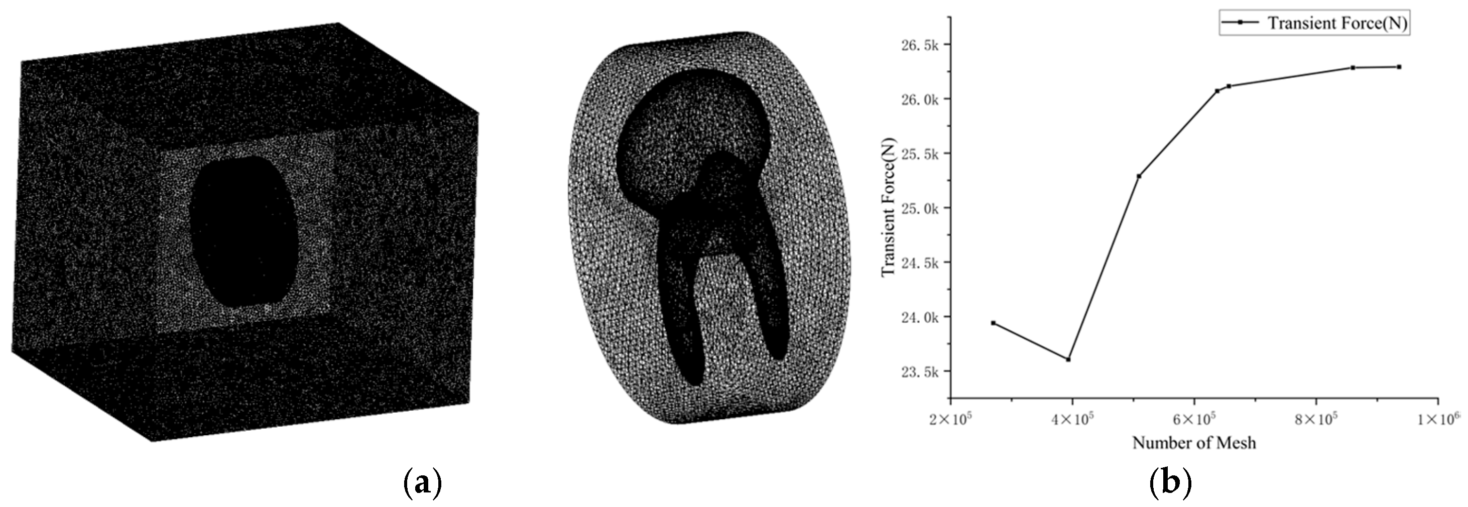
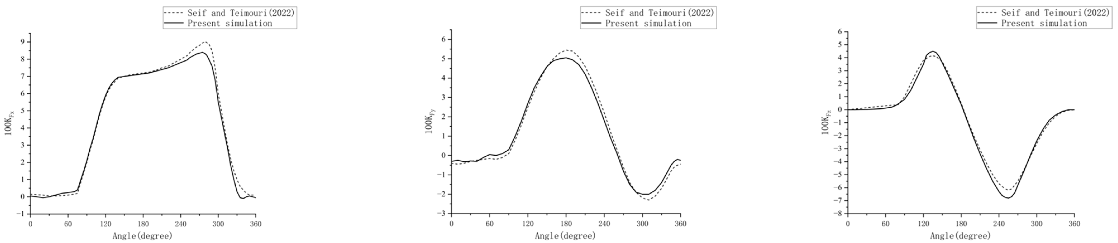
3.3. Meshing and Model Validation

The sliding mesh technique is a common method for simulating unsteady flow fields in rotating machinery. The computational fluid domain is typically partitioned into rotating and stationary regions, with mesh sliding at their interface. This study involved the transfer of flow field information by interpolating physical quantities across the interface. Although it was not necessary for the meshes on either side of the interface to be aligned, minimizing their scale was imperative to prevent the emergence of significant gaps within the flow field during computations. The entire flow field was bifurcated into two distinct regions: an interior cylindrical rotating zone that encompassed the partially submerged propeller, and an exterior stationary region. The interior region featured a dense, unstructured mesh pattern to accurately represent the complex geometric shapes and substantial variations in the flow fields. In contrast, the exterior region utilized a sparse, structured mesh. The entire flow field was meshed using advanced mesh control techniques based on proximity and curvature. The mesh distortion degree was set to 0.7 and hybrid meshes were adopted to reduce the total number of meshes. Locally, mesh refinement was implemented in close proximity to the free liquid surfaces and at the sliding interface.

During the numerical simulation, the number of meshes was subjected to an independent verification to ensure the accuracy of the calculation results. Seven different numbers of meshes were set up, and the transient forces on different numbers of meshes at the same time were monitored and compared. The meshing diagram and the results of the mesh independence verification are depicted in Figure 6. Ultimately, 6.3 × 10⁵ was selected as the most appropriate number of meshes, with the mesh size averaging at 8.4 × 10⁻⁴ m.

After completing the grid independence verification, the numerical calculation method employed in this study was further rigorously validated. By reproducing the numerical simulation under the working conditions of an immersion ratio of 0.4 and an advance ratio of 0.8, as presented in the article by Seif and Teimour [31], the obtained data (K_Fx, K_Fy, K_Fz) were compared and analyzed against the data illustrated in Figure 19 of the reference. The results, processed using the dimensionless method described in the article, demonstrate a high degree of agreement between the calculated results and the reference data, confirming the reliability of the numerical simulation method used in this study. This provides a solid theoretical foundation and methodological support for subsequent research. The comparison is shown in Figure 7.

3.4. Boundary Conditions and Initial Conditions

The initial seawater level was set at half the submerged depth of the propeller, ensuring that the simulation commenced from the designated submergence condition. The fluid within the simulation domain was initialized to a quiescent state prior to the initiation of propeller rotation and inflow, facilitating a natural development of the flow field. An inflow method was employed to analyze the motion of the propeller, with an inflow velocity of 26 knots. The rotational dynamics of the rotating region were defined concurrently, with the propeller blade surfaces aligned to rotate with this region. Following the right-hand rule, the direction of rotation was established to be opposite to the fluid velocity, at a rotational speed of 1820 rotations per minute.

The inlet was configured as a velocity inlet, maintaining air pressure at atmospheric levels. The turbulence intensity and the turbulence viscosity ratio at the inlet were set at 0.1% and 1, respectively. These turbulence parameters reflect typical values for low-turbulence, far-field inflow conditions commonly assumed in open water propeller simulations, where detailed upstream turbulence characteristics are either unavailable or not the primary focus. Such low turbulence levels help minimize extraneous disturbances on the propeller inflow.

The outlet was designated as a pressure outlet, ensuring that the pressure and turbulence parameters matched those at the inlet. No-slip boundary conditions were applied to the surfaces of the partially submerged propeller blades and adjacent walls. The interface between the rotating region containing the propeller and the stationary outer domain was handled using a sliding mesh interface. This technique allows for the direct simulation of the propeller’s rotation relative to the stationary domain by interpolating fluxes across the interface, accurately capturing the transient interaction. To achieve precise determination of the rotating position of the partially submerged propeller during post-processing, a fixed time step of 10 × 10⁻⁵ seconds was utilized in the computations.

4. Computation Results and Analysis

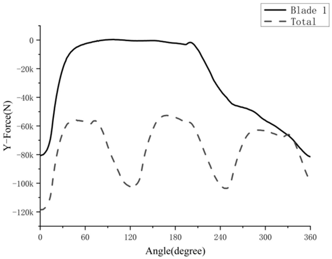
4.1. Force–Time Analysis

The slight pulsations in excitation force due to factors such as wake flow in conventional propellers can be neglected. However, for partially submerged propellers, the alternate water entry of blades causes significant pulsations in the six component forces over time. During the initial rotation of the propeller, the fluid domain experiences unstable flow characterized by irregular pulsations; as the flow field develops, these pulsations in the excitation forces exhibit distinct periodic characteristics.

Due to the periodic entry and exit of each blade in the water and the minimal forces experienced in the air, the blades experienced significant pulsating excitation forces. The numerical simulation results of the excitation forces in the x, y, and z directions of a single blade over one rotation cycle are presented in Figure 8, Figure 9 and Figure 10. In these figures, (i) represents the force and (ii) signifies moment components. As seen from the curves for the x and y directions, the force components along both axes exhibit similar variation characteristics throughout the rotation. This variation can be characterized by the following stages, referencing the points marked on the curves:

Points a–b represent the water-exit phase of the blade.

Points b–c represent the rotation of the blade entirely in the air.

Points c–d represent the water-entry phase of the blade.

Points d–e represent the rotation of the blade fully submerged in water.

This study makes an important observation regarding the acquired curve results. The unsteady fluid analysis employed indicates that the final calculation results can only approach a state of stability. Achieving a condition in which the forces pulsate in a steady manner poses significant challenges.

Figure 8. Pulsation variation curves of force and moment components in the x direction over one cycle.

Figure 8. Pulsation variation curves of force and moment components in the x direction over one cycle.

Figure 9. Pulsation variation curves of force and moment components in the y direction over one cycle.

Figure 9. Pulsation variation curves of force and moment components in the y direction over one cycle.

Figure 10. Pulsation variation curves of force and moment components in the z direction over one cycle.

Figure 10. Pulsation variation curves of force and moment components in the z direction over one cycle.

From Figure 8, Figure 9 and Figure 10, a prominent feature can be observed: the six force components exhibit pronounced pulsation variations, both positive and negative. However, notable disparities exist in the variation characteristics of the curves depicted in Figure 7, Figure 8 and Figure 9, indicating differences in the fluctuations of the force components along the x and y axes versus the z axis. This divergence is primarily attributed to the propeller blades’ interaction with the water surface upon entry, which results in a significant impact in both the x and y directions, leading to a rapid increase in the forces exerted on the blades. Conversely, once the blades emerge from the water and operate in air, the forces acting on them diminish significantly, provoking a sudden decrease in the force components. The force components along the x and y axes display identical variation patterns during the same rotation cycle, which can be delineated into four distinct phases: water exit of the blade (i.e., points a–b), rotation of the full blade in air (i.e., points b–c), water entry of the blade (i.e., points c–d), and rotation of the full blade in water (i.e., points d–e). In contrast, the force components in the z direction do not exhibit significant pulsation during the water-exit and -entry phases. These pulsations can be categorized into two phases: rotation of the blade in water (i.e., points a–b and points c–d), and rotation of the blade in air (i.e., points b–c). In addition, the pulsation variations in force components along the three directions exceeded 50% of the components’ peak values, respectively.

To elucidate the dynamic characteristics of the excitation forces experienced by a single blade (Blade 1, represented by the solid line in the figures) under partially submerged conditions,

Table 1. Key excitation force characteristics for Blade 1 over one cycle.

Force Component (Blade 1)	Symbol	Min. Value (kN)	Max. Value (kN)	Peak-to-Peak (kN)	Pulsation Amplitude (Amp.) (kN)	Amp. as % of Max. Peak Magnitude	Amp. as % of Blade 1 Avg. Thrust
Vertical Force (Fx)	Fx	−18	28	46	23	82.1% (23/28)	57.5% (23/40)
Thrust (Fy)	Fy	−80	0	80	40	50.0% (40/80)	100% (40/40)
Lateral Force (Fz)	Fz	−30	2	32	16	53.3% (16/30)	40.0% (16/40)

summarizes the key parameters of its principal force components, including the maximum and minimum values within each cycle and the derived pulsation characteristics.

As indicated in Table 1, Blade 1 experiences significant load variations throughout its rotational cycle. Its vertical force (Fx) fluctuates approximately between −18 kN and +28 kN, exhibiting a peak-to-peak pulsation as high as 46 kN. The corresponding pulsation amplitude (23 kN) reaches approximately 82.1% of its own positive peak value (28 kN). The lateral force (Fz) varies over a range of approximately −30 kN to +2 kN, with a peak-to-peak pulsation of 32 kN; its pulsation amplitude (16 kN) is approximately 53.3% of the absolute value of its own negative peak (−30 kN). Importantly, this observed pattern of pronounced Fx pulsations, particularly the generation of large positive and negative peaks corresponding to blade immersion and emersion, is qualitatively consistent with the findings of earlier researchers. For instance, Olofsson (1996) [18] reported significant dynamic vertical loads in experimental studies on partially submerged propellers, highlighting the critical impact of the blade’s interaction with the free surface during entry and exit. Similarly, the theoretical framework for surface-piercing propellers developed by Vorus (1991) [11] predicts considerable fluctuations in vertical forces due to asymmetric hydrodynamic loading and ventilation phenomena inherent to this operational mode. The consistency in these general trends supports the accurate representation of the fundamental physics in our current CFD simulation.

Comparing the pulsations of the non-axial forces with the average thrust, the pulsation amplitude of the vertical force on Blade 1 constitutes approximately 57.5% of its average thrust, while that of the lateral force accounts for approximately 40.0%. These results further underscore that, under partially submerged conditions, the excitation forces experienced by a single blade are not only extremely unstable in the primary thrust direction but also possess non-axial dynamic components that are exceptionally significant relative to the average propulsive force.

Similarly, the moment components acting on Blade 1 also exhibit pronounced dynamic characteristics analogous to those observed for the force components. This forms a fundamental basis for understanding the complex excitation characteristics of the entire propeller.

The excitation forces on individual blades exhibited consistent periodicity and amplitude, albeit with phase variations among blades. Summing these forces yielded the six distinct components of the total propeller excitation forces illustrated in Figure 11.

Figure 11 illustrates that the overall propeller excitation force exhibits significant pulsation, although its magnitude remains lower than that of an individual blade. The pulsation cycle of the total force is one-third that of a single blade. Furthermore, the force components in the x and z directions exhibit variation patterns similar to those in the y direction. Analysis of these curves reveals that the partially submerged propeller undergoes substantial pulsations and frequent directional changes in the three orthogonal force components (x, y, and z) during operation. These fluctuations could potentially have a negative influence on the shafting’s dynamic response characteristics. This possibility should be fully considered in the design of shafting devices for partially submerged propellers in high-speed boats.

These significant temporal pulsations highlight the dynamic nature of the loading. To further understand their potential impact and how these forces are oriented in space, the directional characteristics of these excitation forces are examined below.

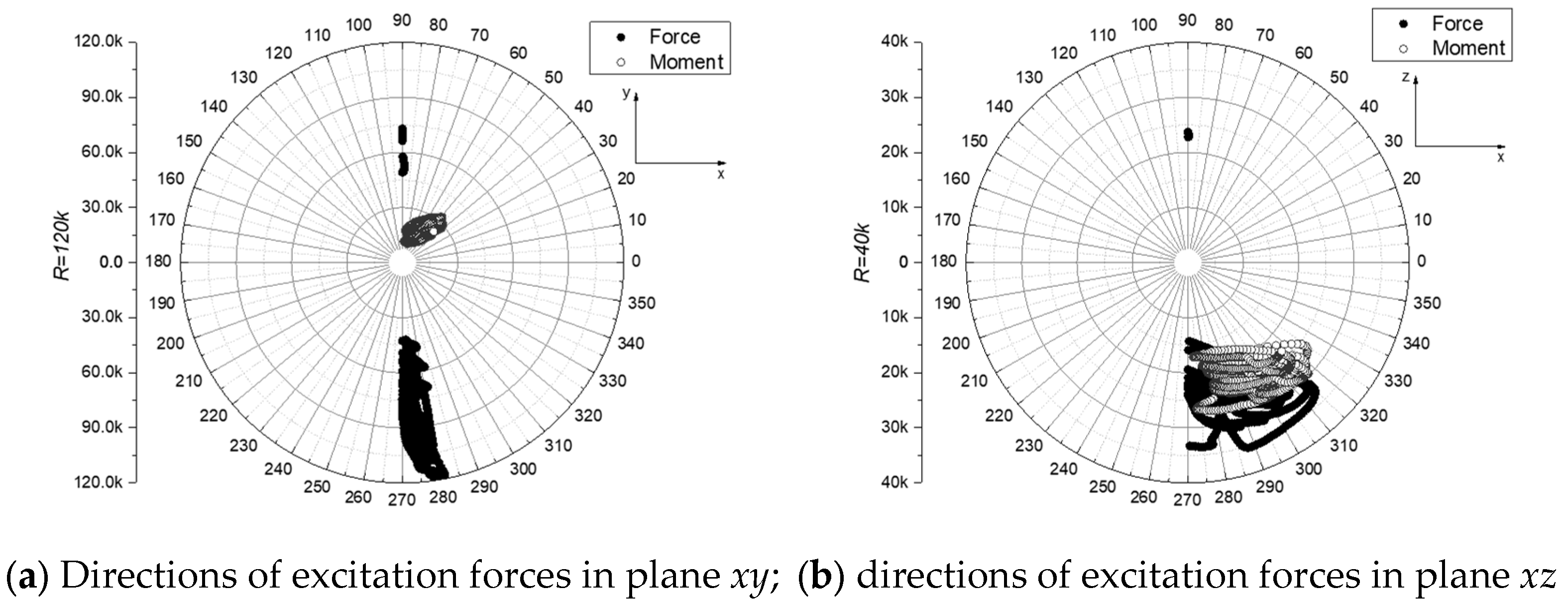
4.2. Vector Orientation

This section examines the directionality of excitation forces within three mutually perpendicular spatial coordinate planes, as pronounced fluctuations during propeller operation adversely affect vessel maneuverability. The three reference planes are defined as follows: the horizontal plane (zy plane) and two vertical planes (xy plane and xz plane). To characterize force directionality, propeller excitation force vectors were paired within these planes. Polar coordinate representations of these pairings are shown in Figure 12 and Figure 13.

In the horizontal plane (zy), the excitation forces exhibit a dispersed directionality. These concentrated forces fluctuate from 10° to 25° to the left of the propeller shaft alignment, while the moments vary from 30° to 60° towards the left in the shaft’s negative vector direction. Similarly, in the vertical plane (xy), the excitation forces display comparable directional distribution characteristics. However, the moments in this plane concentrate predominantly rightward relative to the shaft’s negative direction. In the vertical plane (xz), forces distribute more widely, with both forces and moments predominantly ranging from 0° to 45° to the right of the −z direction (lateral to the propeller shaft).

The pronounced fluctuations in vertical and lateral excitation forces, arising from the operational characteristics of the partially submerged propeller, result in a significant proportion of forces in these two directions relative to the total forces acting on the propeller. This phenomenon can adversely affect the directional stability and maneuverability of the boat. In marine applications, the propeller shaft can be adjusted for specific tilt angles and axial skew flow angles. By optimizing the contributions from lateral and axial forces in alignment with the vessel’s heading, adverse impacts on the vessel’s handling characteristics and course-keeping ability can be mitigated. Optimal angle configurations should be determined via comprehensive analysis of vessel types and propeller geometries to enhance maneuvering performance.

This dispersed and fluctuating directional nature of the resultant forces underscores the complexity of the loading. To gain insight into how these overall force vectors arise from the combined, phased contributions of individual blades as they cycle through air and water, a visualization of these contributions is now presented.

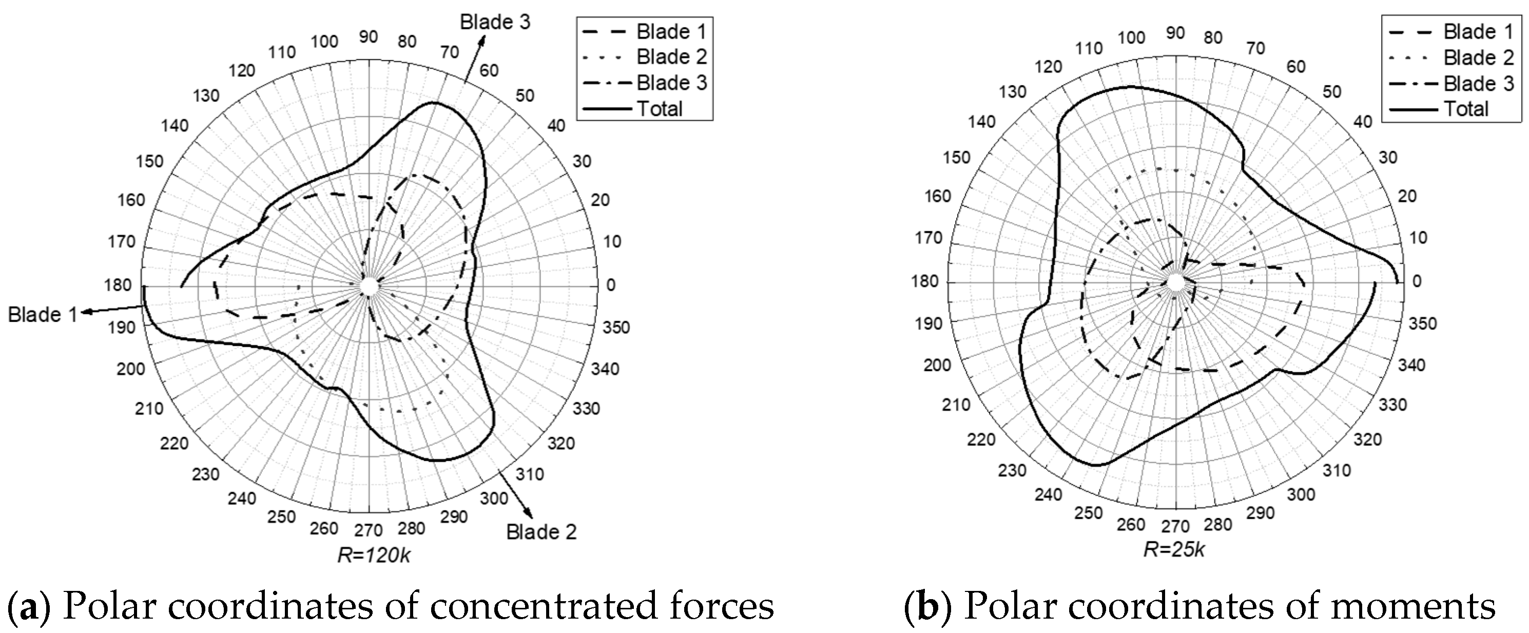
4.3. Analysis of Phase Relationships in Excitation Forces and Visualization of Blade Contributions

As previously indicated, initial propeller rotation generates markedly unstable flow with irregular pulsations. As the flow field develops, however, distinct periodic patterns emerge in the excitation forces. Understanding the phase relationship between the forces on individual blades and the resultant forces on the entire propeller is crucial. This section explores a visualization approach, using polar coordinates, to illustrate these phase relationships and how individual blade loading events contribute to the overall propeller excitation.

Figure 14 displays the polar coordinates transformed from the data in Figure 11 (Comparison between the pulsation variation curves for force components of an individual blade and the overall propeller in the y direction over one cycle) and the corresponding pulsation variations in y-direction moment components of an individual blade and the overall propeller over one cycle.

Figure 14 visually correlates the fluctuation curves of individual blade forces (dashed lines) with that of the total propeller force (solid line). It can be observed that the peak of the total propeller force curve aligns with the successive peak contributions from individual blades. For instance, the vertex of the total propeller force curve corresponds to the instance where a particular blade (or a combination of blades) is experiencing its maximum loading within the water. By mapping these force peaks onto the known angular progression of the propeller (derived from the CFD’s prescribed rotation), one can visualize the approximate angular phase at which these peak loading events occur. For this three-bladed propeller, individual blade peaks occur at approximately 120° intervals. This visualization elucidates how phased blade water-entry/exit events generate the global cyclic loading pattern. It is a visual aid for interpreting CFD output, rather than an independent method for determining blade position, as the latter is an input to the simulation.

5. Conclusions and Future Work

This study conducted a computational analysis of the excitation forces generated by partially submerged propeller(s) on a high-speed boat using CFD. The study focused on deriving periodic pulsation variation curves for six force components driving excitation in three directions in the propeller rotation process. The computational analysis yielded the following insights:

(1)

This study outlined theoretical computational considerations for assessing propeller performance, grounded in fluid dynamics principles related to water entry. A numerical simulation model was subsequently employed to investigate the periodic characteristics of six force components (in the shaft, vertical, and lateral directions) of a partially submerged propeller under the simulated conditions.

(2)

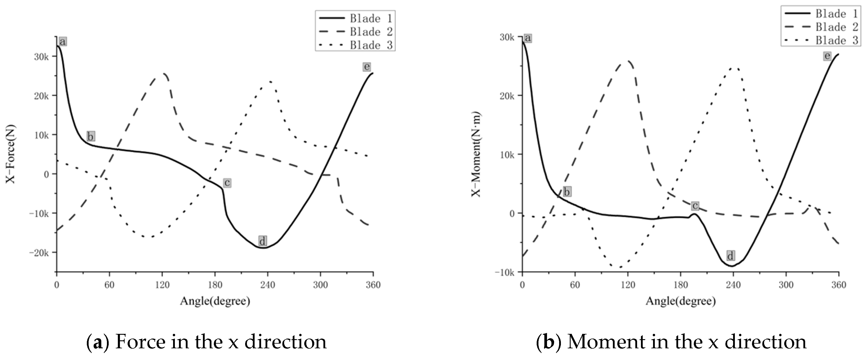
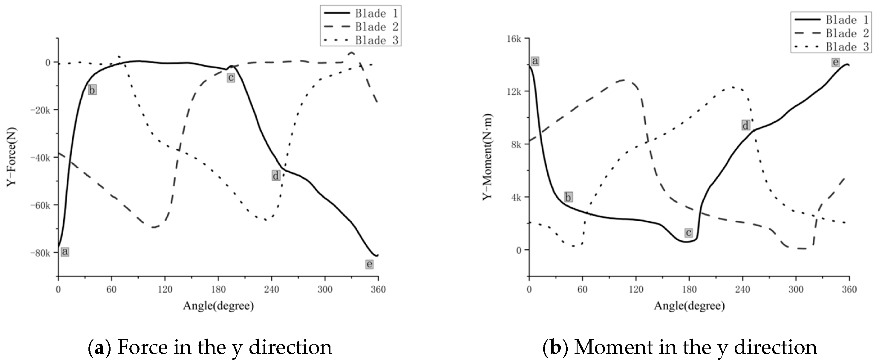
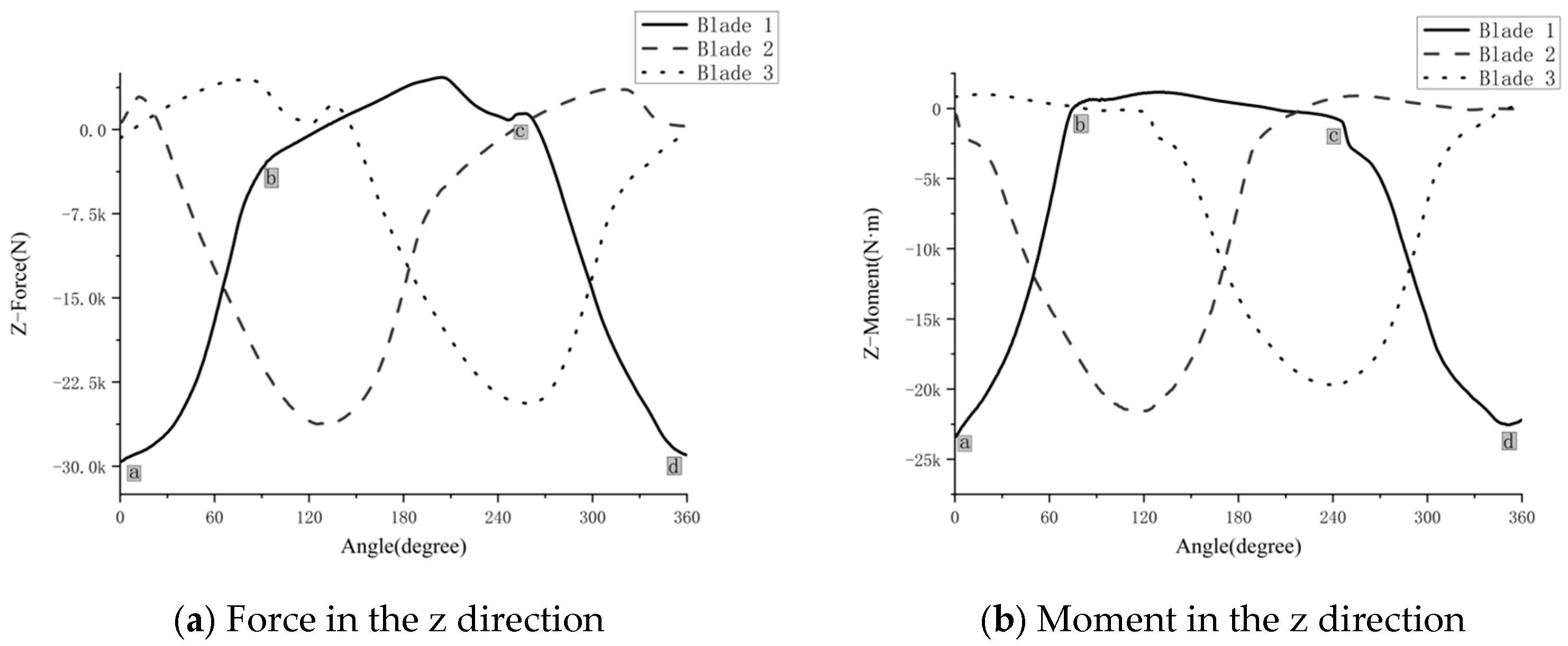
The excitation loads (encompassing both forces and moments) acting on a single blade of the partially submerged propeller, as characterized by the current CFD model, exhibited highly dynamic characteristics under the simulated conditions. Pulsation amplitudes of the non-axial forces and bending moments were observed to often reach levels corresponding to 50–80% of their respective peak magnitudes. Such pronounced, multi-axial, and unsteady loads, identified in this computational exploration, are considered potentially significant dynamic inputs to the shafting system.

(3)

A visualization technique using polar coordinates was utilized to explore the simulated phase relationships between individual blade excitation forces and the total propeller forces. This approach may offer a means to better understand how the sequential loading of blades, based on their angular positions derived from the CFD simulation, could contribute to the overall periodic excitation patterns observed.

While the present study provides detailed insights into the excitation force characteristics of the analyzed partially submerged propeller configuration, its foundation primarily rests on qualitative CFD analysis and a representative single-case investigation. Extending these quantitative findings to other designs or broader operational conditions would require comprehensive parametric studies and experimental validation. Investigating a range of submergence ratios (h/D), propeller geometric variations (e.g., pitch, skew, blade area ratio, blade count), different inflow velocities (varying advance coefficient J and Reynolds number), and potentially shaft inclination angles is crucial for developing more generalized predictive models and design guidelines for mitigating adverse shafting vibrations induced by partially submerged propellers. Furthermore, applying the calculated excitation forces as input to a coupled fluid–structure interaction analysis or a dynamic shafting system model represents a necessary next step to directly quantify the vibrational response.

References

1. Chaitanya, N.; Murthy, Y.S.; Madaka, R.M.M.R.; Balaji, R.; Narayanan, J.; Hulmani, R.M. Vibrartion Analysis of Fibre Glass Contra Rotating Propeller of Fishing Vessel. In Proceedings of the OCEANS 2022—Chennai, Chennai, India, 21–24 February 2022; pp. 1–5. [Google Scholar]
2. Tian, J.; Zhang, Z.; Ni, Z.; Hua, H. Flow-induced vibration analysis of elastic propellers in a cyclic inflow: An experimental and numerical study. Appl. Ocean Res. 2017, 65, 47–59. [Google Scholar] [CrossRef]
3. Zhu, J.C.; Zhu, H.H.; Yan, X.P.; Jiang, P. A Research on the Influence of Vessel-Propeller Coupling Effect to Shaft’s Lateral Vibration. Appl. Mech. Mater. 2012, 226–228, 106–112. [Google Scholar] [CrossRef]
4. Javanmardi, N.; Ghadimi, P. Hydroelastic analysis of a semi-submerged propeller using simultaneous solution of Reynolds-averaged Navier–Stokes equations and linear elasticity equations. Proc. Inst. Mech. Eng. Part M J. Eng. Marit. Environ. 2018, 232, 199–211. [Google Scholar] [CrossRef]
5. Chen, Y.; Wang, L.; Hua, H. Longitudinal vibration of marine propeller-shafting system induced by inflow turbulence. J. Fluids Struct. 2017, 68, 264–278. [Google Scholar] [CrossRef]
6. Huang, Q.; Yan, X.; Zhang, C.; Zhu, H. Coupled transverse and torsional vibrations of the marine propeller shaft with multiple impact factors. Ocean Eng. 2019, 178, 48–58. [Google Scholar] [CrossRef]
7. Jiang, X.; Zhou, X.; Chen, K. Vibration characteristics of a marine propulsion shaft excited by the effect of propeller and diesel. In Proceedings of the 2015 International Conference on Transportation Information and Safety (ICTIS), Wuhan, China, 25–28 June 2015; pp. 893–897. [Google Scholar]
8. Huang, Q.; Xia, J.; Liu, H. Friction-induced vibration of marine propeller shaft based on the LuGre friction model. J. Mech. Sci. 2023, 37, 3867–3876. [Google Scholar]
9. Furuya, O. A performance-prediction theory for partially submerged ventilated propellers. J. Fluid Mech. 1985, 151, 311–335. [Google Scholar] [CrossRef]
10. Young, Y. Numerical Modeling of Supercavitating and Surface-Piercing Propellers. Ph.D. Thesis, The University of Texas at Austin, Austin, TX, USA, 2002. [Google Scholar]
11. Vorus, W.S. Forces on Surface-Piercing Propellers with Inclination. J. Ship Res. 1991, 35, 210–218. [Google Scholar] [CrossRef]
12. Lewis, E.V. Principles of Naval Architecture; Society of Naval Architects and Marine Engineers: Jersey City, NI, USA, 1989; Volume 2, Chapter 7. [Google Scholar]
13. Kudo, T.; And Ukon, Y. Calculation of supercavitating propeller performance using a vortex-lattice method. In Proceedings of the 2nd International Symposium on Cavitation, Tokyo Japan, 5–7 April 1994; pp. 403–408. [Google Scholar]
14. Kudo, T.; And Kinnas, S. Application of vortex/source lattice method on supercavitating propellers. In Proceedings of the 24th American Towing Tank Conference, College Station, TX, USA, 2–3 November 1995. [Google Scholar]
15. Savineau, C.; And Kinnas, S. A numerical formulation applicable to surface piercing hydrofoils and propellers. In Proceedings of the 24th American Towing Tank Conference, College Station, TX, USA, 2 November 1995. [Google Scholar]
16. Rose, J.C. Methodical series model test results. In Proceedings of the Fast ’91, 1st International Conference on Fast Sea Transportation, Trondheim, Norway, 17–21 June 1991. [Google Scholar]
17. Olofsson, N.A. Contribution on the Performance of Partially Submerged Propellers. In Fast ’93, 2nd International Conference on Fast Sea Transportation, Yokohama, Japan, 13–16 December 1993; Sponsored by Min Transport, Japan & Sasakawa Foundation; Japan Society of Naval Architects and Ocean Engineers: Tokyo, Japan, 1993; Volume 1, p. 765. ISBN 4-930966-00-0. [Google Scholar]
18. Olofsson, N. Force and Flow Characteristics of a Partially Submerged Propeller. Ph.D. Thesis, Department of Naval Architecture and Ocean Engineering, Chalmers University of Technology, Göteborg, Sweden, February 1996. [Google Scholar]
19. Miller, W.; Szantyr, J. Model experiments with surface piercing propellers. Schiffstechnik 1998, 45, 14–21. [Google Scholar]
20. Caponnetto, M. RANSE simulations of surface piercing propellers. In Proceedings of the 6th Numerical Towing Tank Symposium, Rome, Italy, 29 September–1 October 2003. [Google Scholar]
21. Kinnas, S.; And Fine, N. A nonlinear boundary element method for the analysis of unsteady propeller sheet cavitation. In Proceedings of the 19th Symposium on Naval Hydrodynamics, Seoul, Republic of Korea, 23–28 August 1992; pp. 717–737. [Google Scholar]
22. Young, Y.L.; Kinnas, S.A. A BEM for the prediction of unsteady midchord face and/or back propeller cavitation. J. Fluids Eng. 2001, 123, 311–319. [Google Scholar] [CrossRef]
23. Young, Y.L.; Kinnas, S.A. Numerical modeling of supercavitating propeller flows. J. Ship Res. 2003, 47, 48–62. [Google Scholar] [CrossRef]
24. Kinnas, S.; Choi, J.; Lee, H.; And Young, J. Numerical cavitation tunnel, Proceedings, NCT50. In Proceedings of the International Conference on Propeller Cavitation, Newcastle upon Tyne, UK, 3–5 April 2000. [Google Scholar]
25. Choi, J. Vortical Inflow-Propeller Interaction Using Unsteady Three-dimensional Euler Solver. Ph.D. Thesis, Department of Civil Engineering, The University of Texas at Austin, Austin, TX, USA, August 2000. [Google Scholar]
26. Shiba, H. Air-Drawing of Marine Propellers; Technical Report 9; Transportation Technical Research Institute: Istanbul, Turkey, 1953. [Google Scholar]
27. Brandt, H. Modellversuche mit schiffspropellern an der wasseroberfläche. Schiff Und Hafen 1973, 5, 415–422. [Google Scholar]
28. Kinnas, S.A.; Fine, N.E. A numerical nonlinear analysis of the flow around two- and three-dimensional partially cavitating hydrofoils. J. Fluid Mech. 1993, 254, 151–181. [Google Scholar] [CrossRef]
29. Fine, N.E. Nonlinear Analysis of Cavitating Propellers in Nonuniform Flow. Ph.D. Thesis, Department of Ocean Engineering, Massachusetts Institute of Technology, Cambridge, MA, USA, October 1992. [Google Scholar]
30. Yakhot, V.; Orszag, S.A. Renormalization group analysis of turbulence. I. Basic theory. J. Sci. Comput. 1986, 1, 3–51. [Google Scholar] [CrossRef]
31. Seif, M.S.; Teimouri, M. Experimental and numerical investigation of hydrodynamic performance of a new surface piercing propeller family. Ocean Eng. 2022, 264, 112161. [Google Scholar] [CrossRef]
Figure 1. Schematic diagram for the influence of a general inflow wake on a partially submerged propeller. The diagram shows the fixed coordinate system (X, Y, Z) of the blade and the fixed coordinate system (X, Y, Z) of the boat.
Jmse 13 01169 g001
Figure 2. Definition of the tip submergence ratio (h/D) and local non-orthogonal curvilinear coordinates (s, v, n).
Jmse 13 01169 g002
Figure 3. Definition of the “exact” and approximate flow boundaries surrounding the blade cross-section of a partially submerged propeller.
Jmse 13 01169 g003
Figure 4. Sketch map of the negative image approach for the blade cross-section of a partially submerged propeller.
Jmse 13 01169 g004
Figure 5. Fluid domain model and its spatial coordinates.
Jmse 13 01169 g005
Figure 6. Meshing diagram (a) and Mesh independence verification (b).
Jmse 13 01169 g006
Figure 7. Comparison between present simulation and reference data (Adapted from [31]).
Jmse 13 01169 g007
Figure 11. Comparison between the pulsation variation curves for force components of a single blade and the overall propeller in the y direction over one cycle.
Jmse 13 01169 g011
Figure 12. Directions of excitation forces in the horizontal plane (zy).
Jmse 13 01169 g012
Figure 13. Directions of excitation forces in vertical planes.
Jmse 13 01169 g013
Figure 14. Polar coordinates of pulsation variations in excitation force components of an individual blade and the overall propeller in the y direction over one cycle.
Jmse 13 01169 g014