
Capacity Estimation of Lithium-Ion Battery Systems in Fuel Cell Ships Based on Deep Learning Model

Abstract
1. Introduction
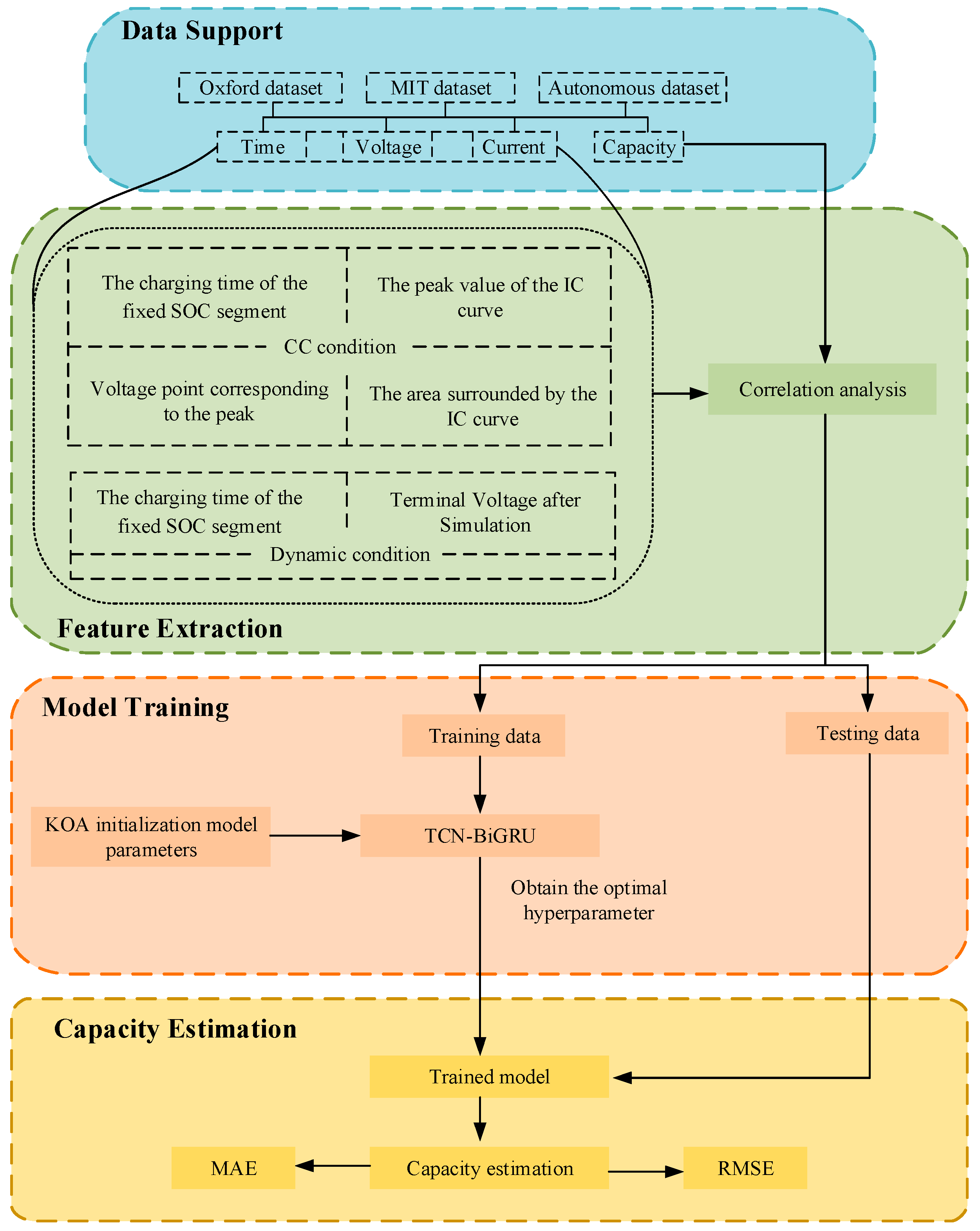
2. Battery Experiment Data and the KOA-TCN-BiGRU Model
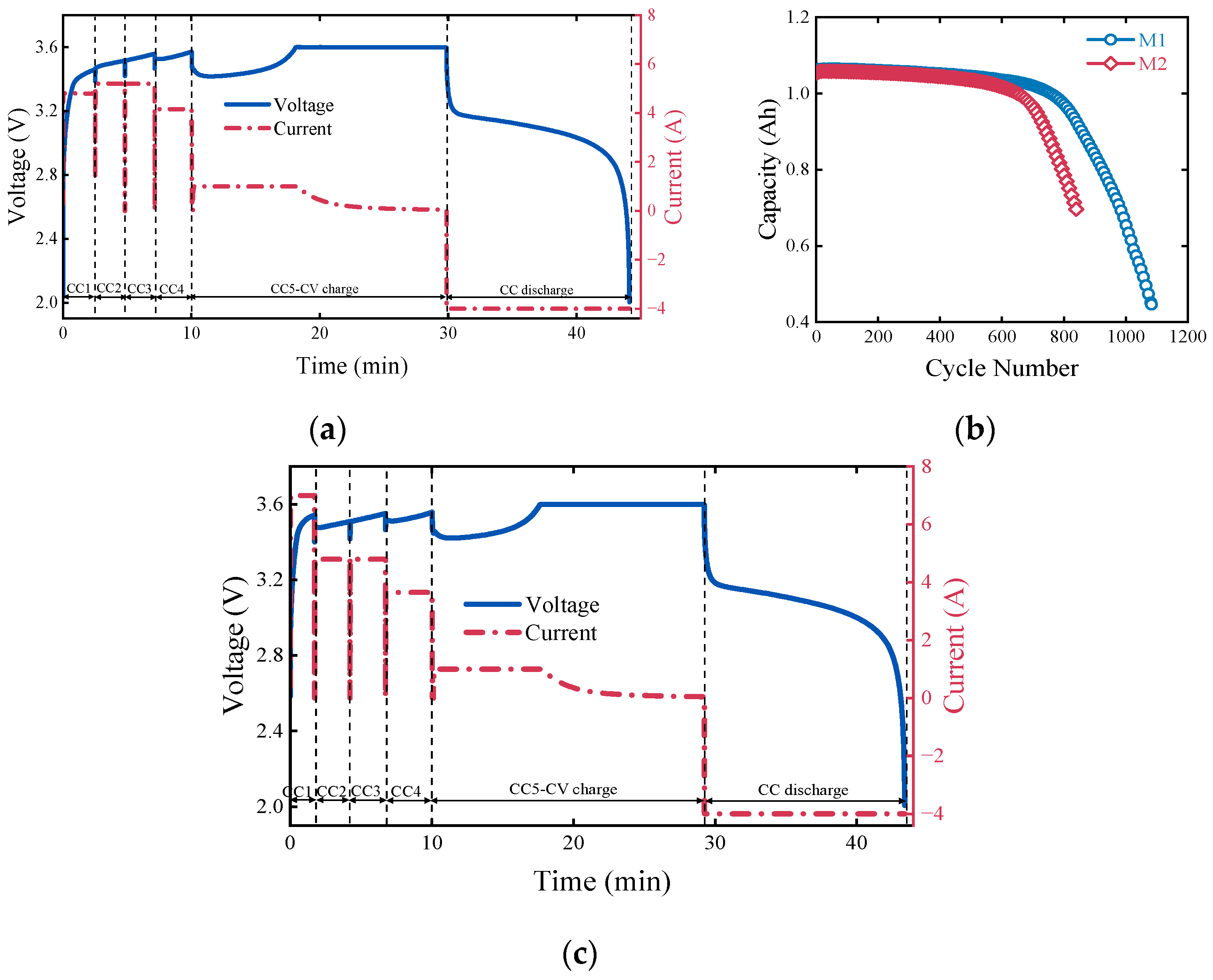
2.1. MIT Battery Dataset
2.2. Oxford Dataset
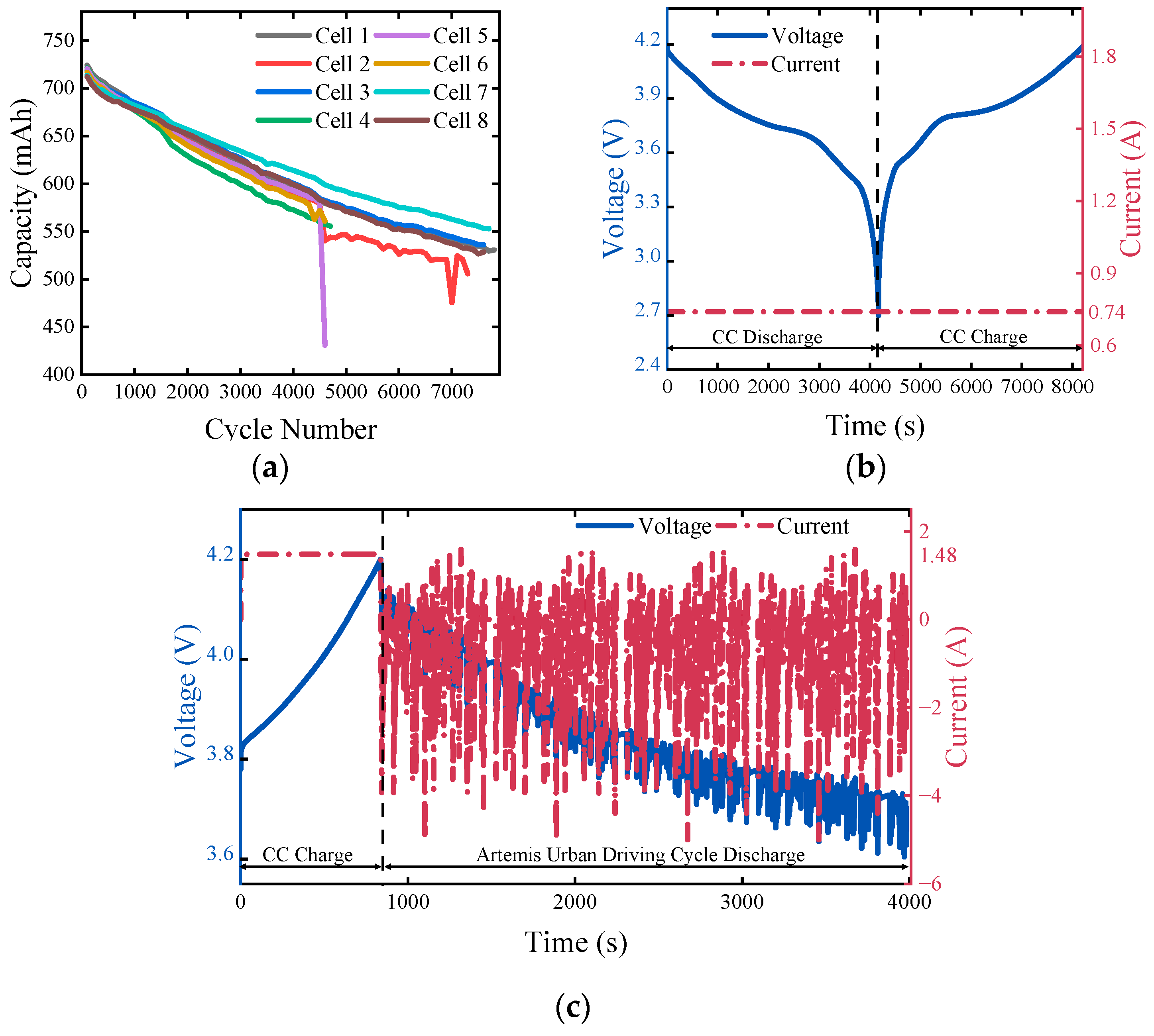
2.3. Battery Aging Experiment Under Simulated Ship Sailing Conditions
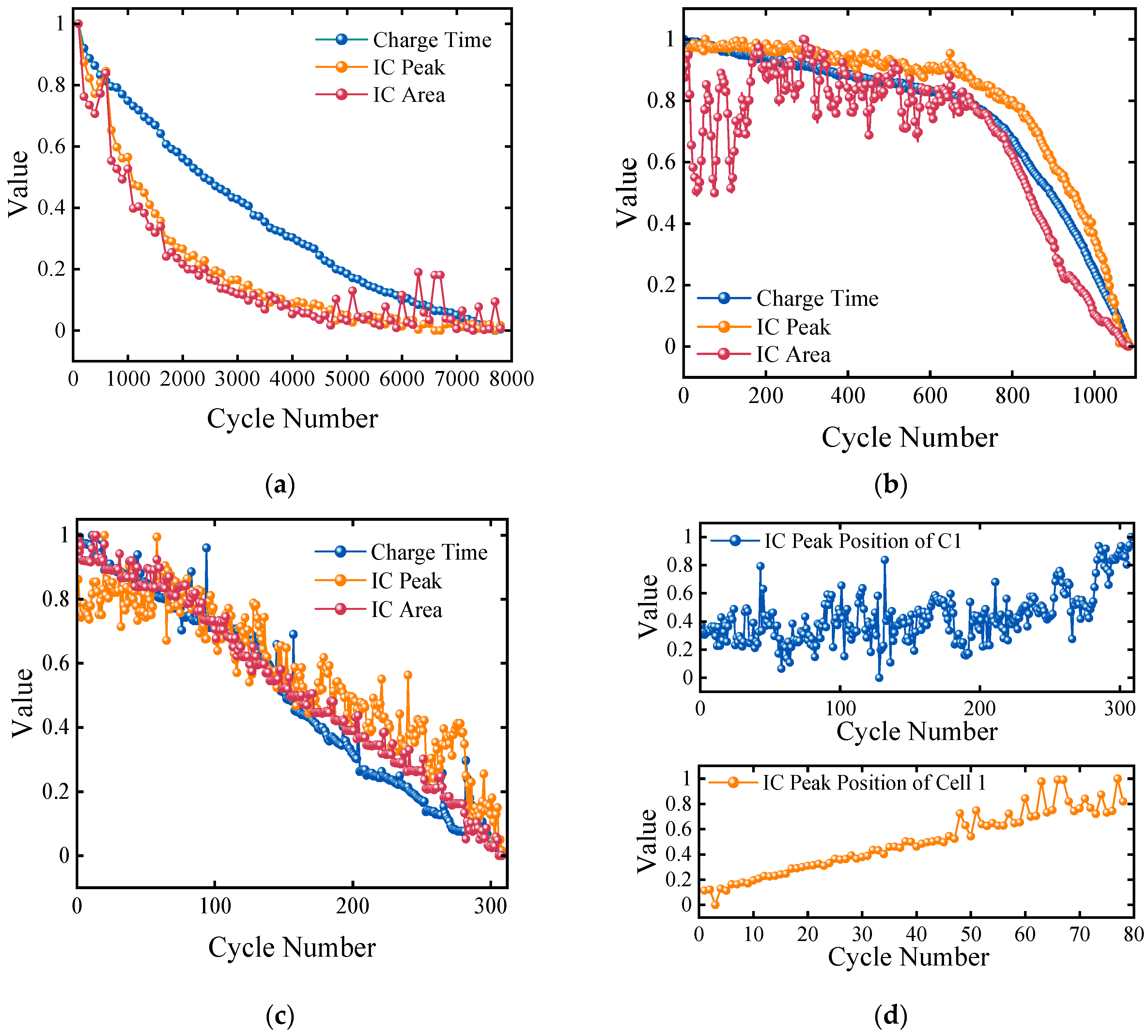
2.4. Data Analysis
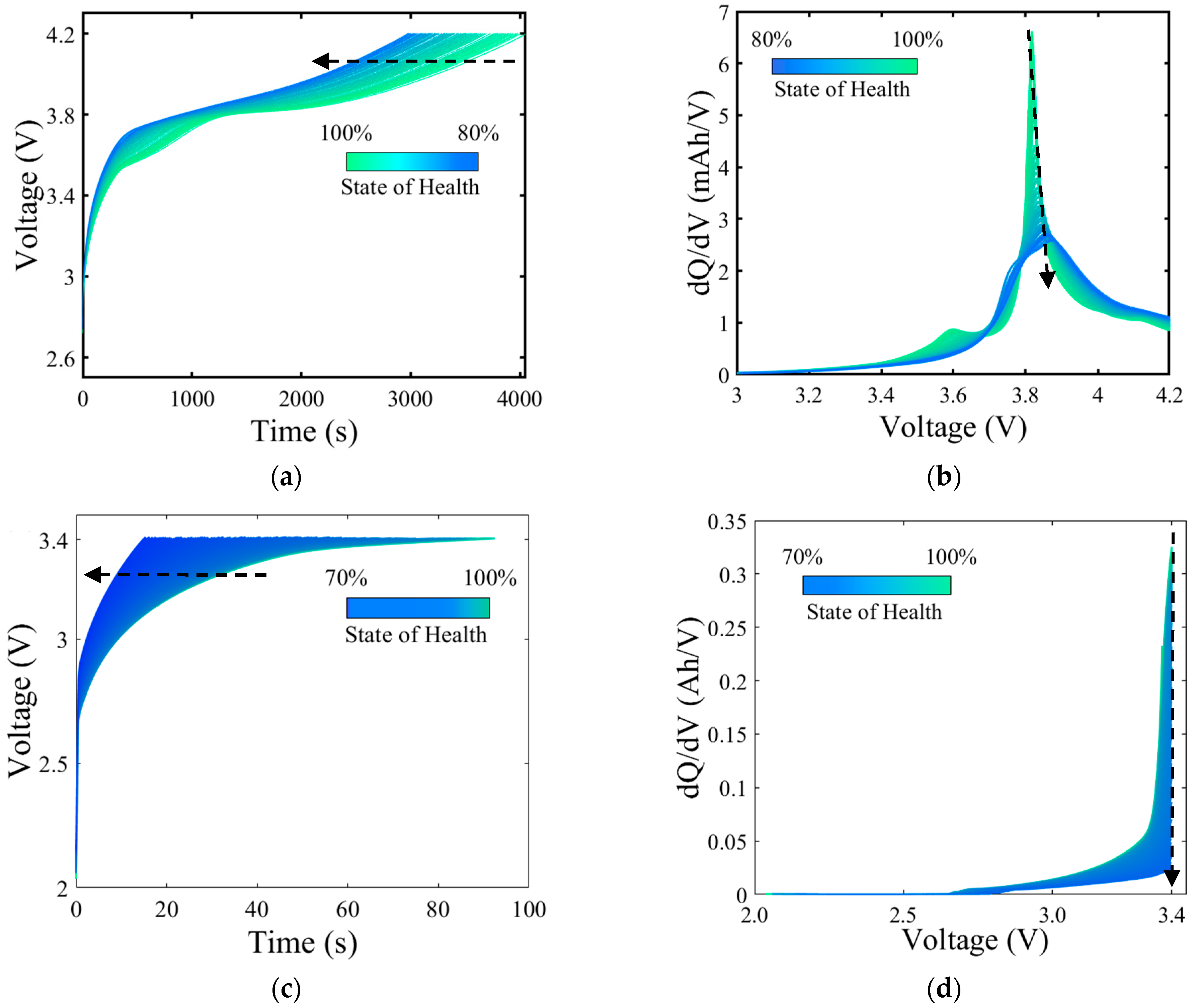
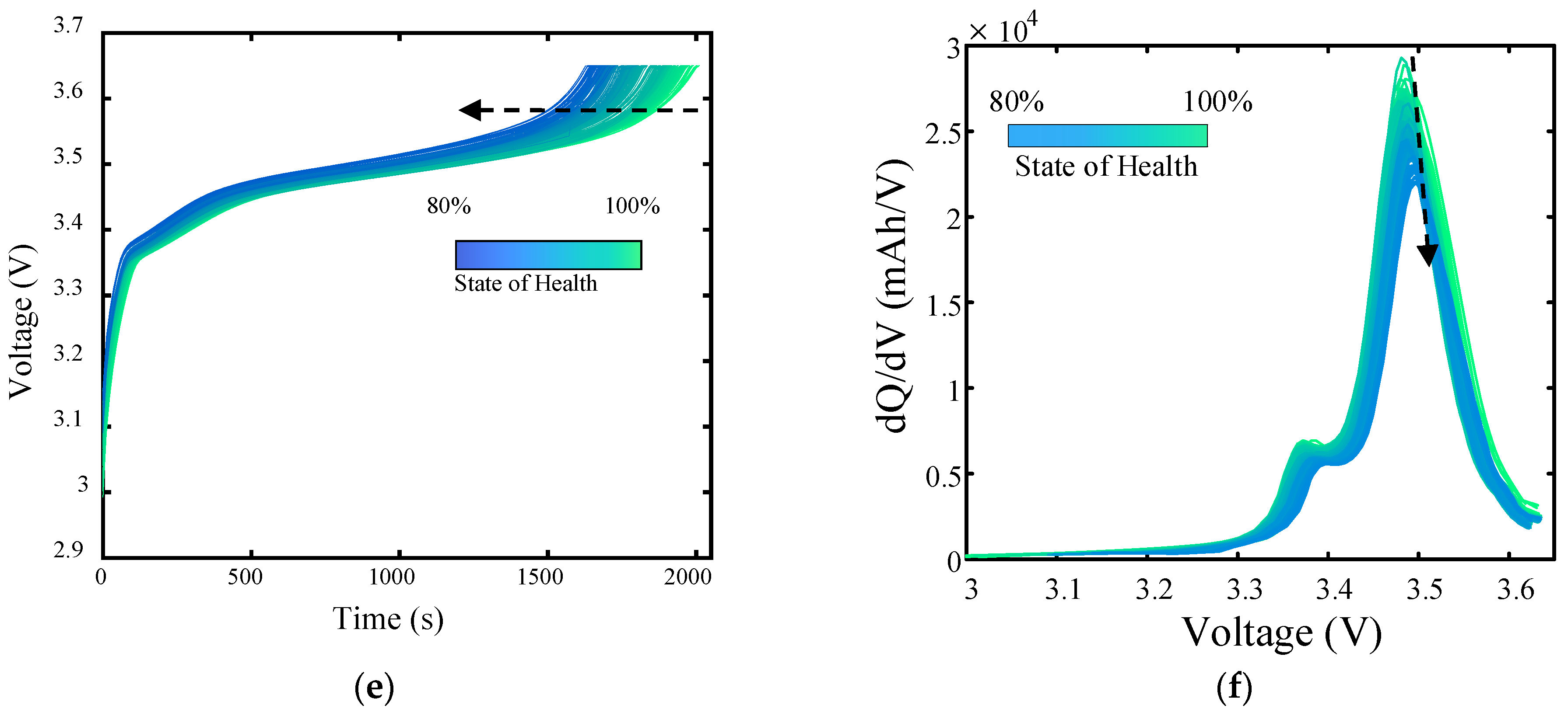
2.4.1. Method of Extracting Universal Health Factors During the Charging Phase
2.4.2. Extraction of Universal Health Factors During the Dynamic Discharging Phase
2.4.3. Correlation Analysis
2.5. The KOA-TCN-BiGRU Method
2.5.1. KOA
- Step 1: Initialization
- Step 2: Defining the Gravitational Force
- Step 3: Calculating an Object’s Velocity and Updating Objects’ Positions
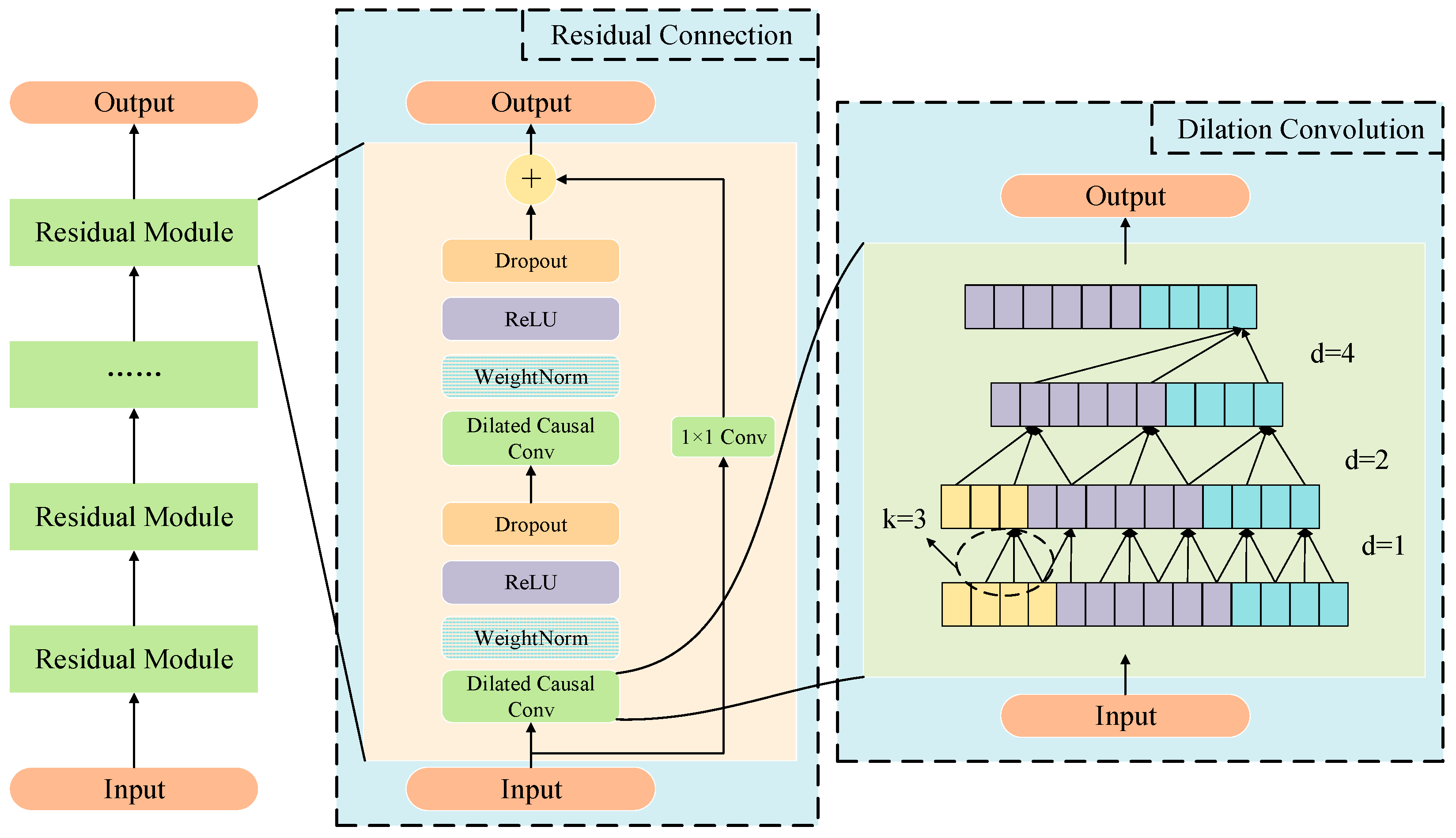
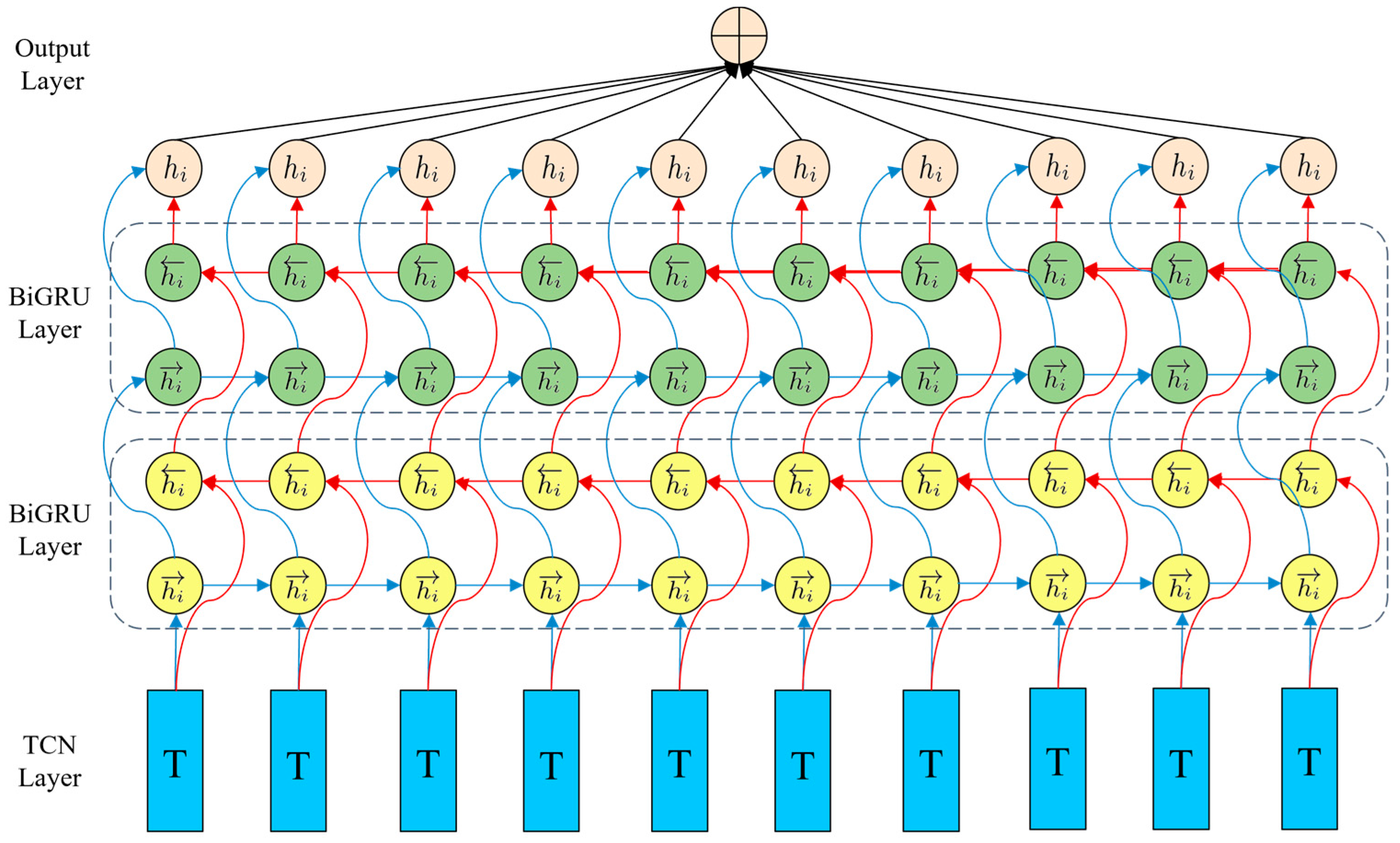
2.5.2. TCN
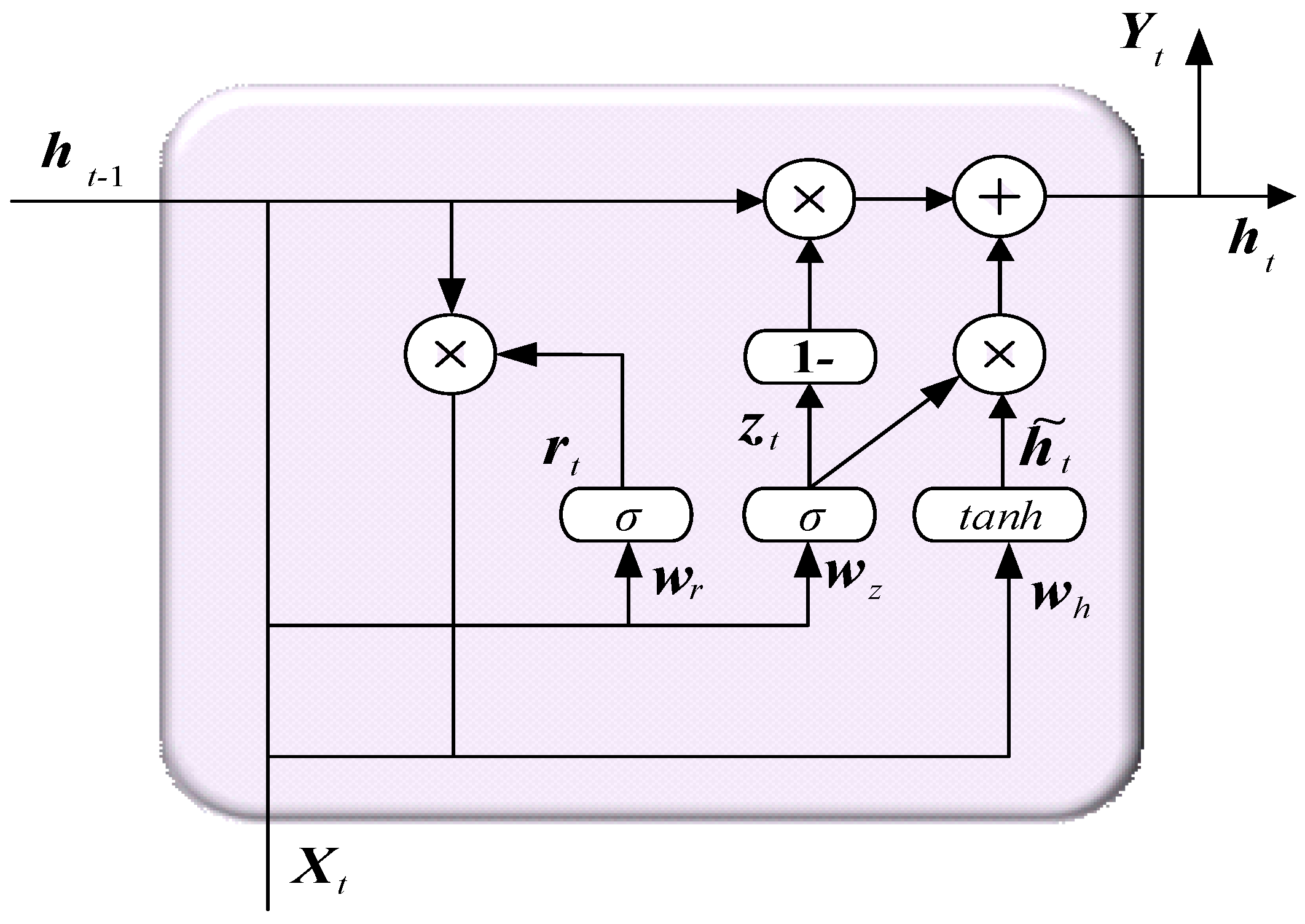
2.5.3. BiGRU
2.5.4. Estimation Process
- (1)
- Input layer: the sequenceInputLayer(f) function is used, where = 4;
- (2)
- TCN module: two causal convolution blocks with dilation factors = 1, 2; each block includes a “convolution1dLayer”, a “layerNormalizationLayer”, a “dropoutLayer” and residual connections via an “additionLayer”; number of filters: 64; kernel size: 5; dropout rate: 0.005;
- (3)
- BiGRU module: two GRU layers of size 35—one for the forward sequence, one for the backward sequence (via “FlipLayer”); the outputs were concatenated with the “concatenationLayer”;
- (4)
- Output layer: a fully connected layer followed by the “regressionLayer”.
2.6. Uncertainty Analysis
- (1)
- Voltage/current sampling resolution: limited by the analog-to-digital converter (ADC) precision, small-amplitude signals (e.g., low-current charging phases) may introduce quantization errors, potentially distorting the incremental capacity (IC) curves and derived health factors (HF1–HF4).
- (2)
- Thermal drift in sensors: ambient temperature control during the experiments was maintained at 30 ± 1 °C for the MIT datasets and at 10–15 °C for the “Jun Lv Hao” simulation [24,25]; fluctuations beyond this range could alter battery impedance and capacity, leading to inconsistent health factor extraction.
- (3)
- Contact resistance in test fixtures: intermittent electrical connections during long-term cycling tests may cause abrupt voltage drops, misattributed as capacity degradation in the model.
3. Results
3.1. Evaluation Criteria
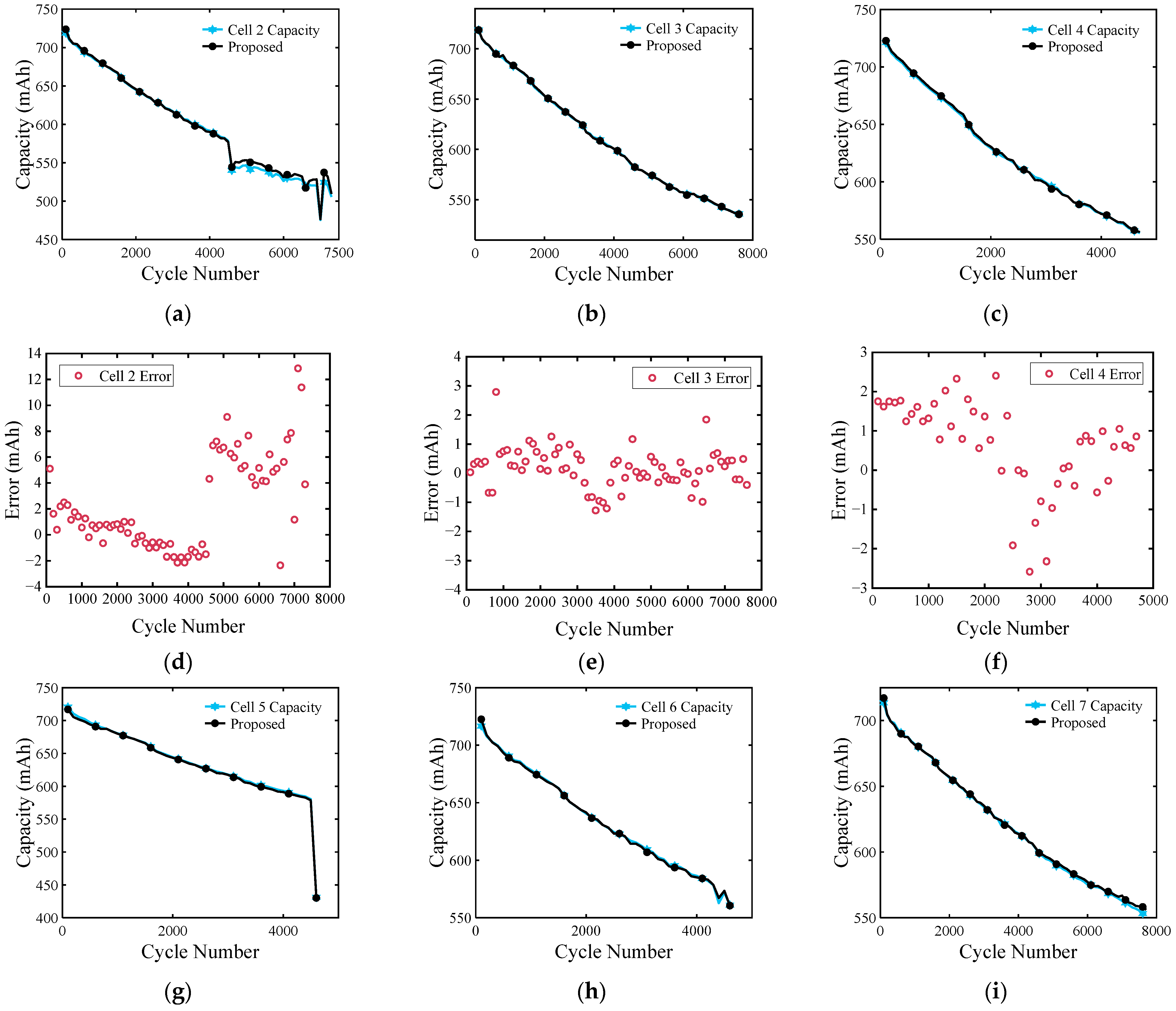
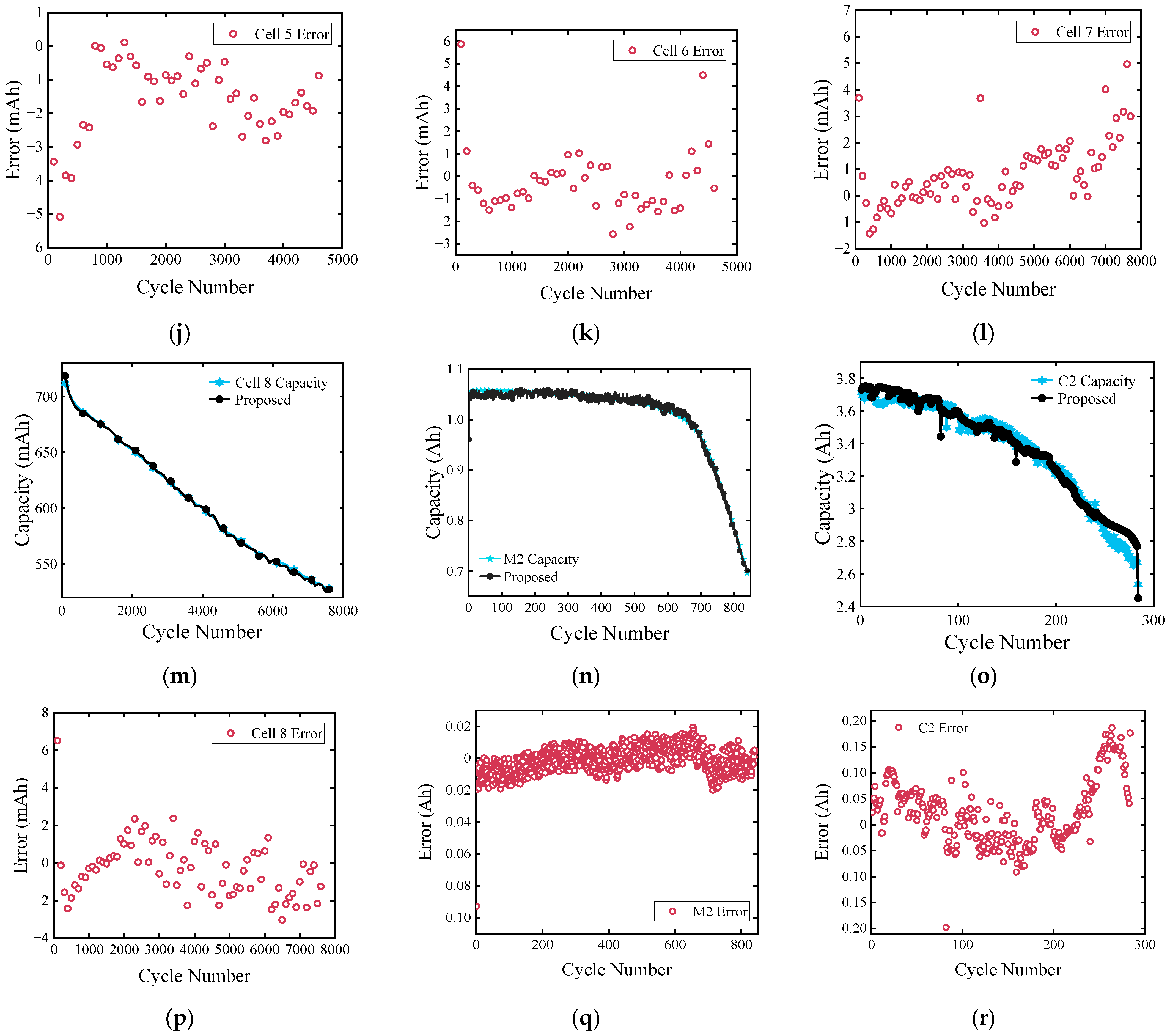
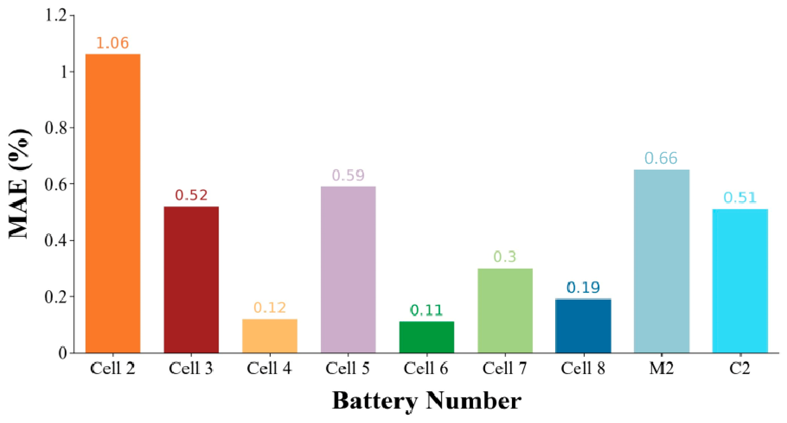
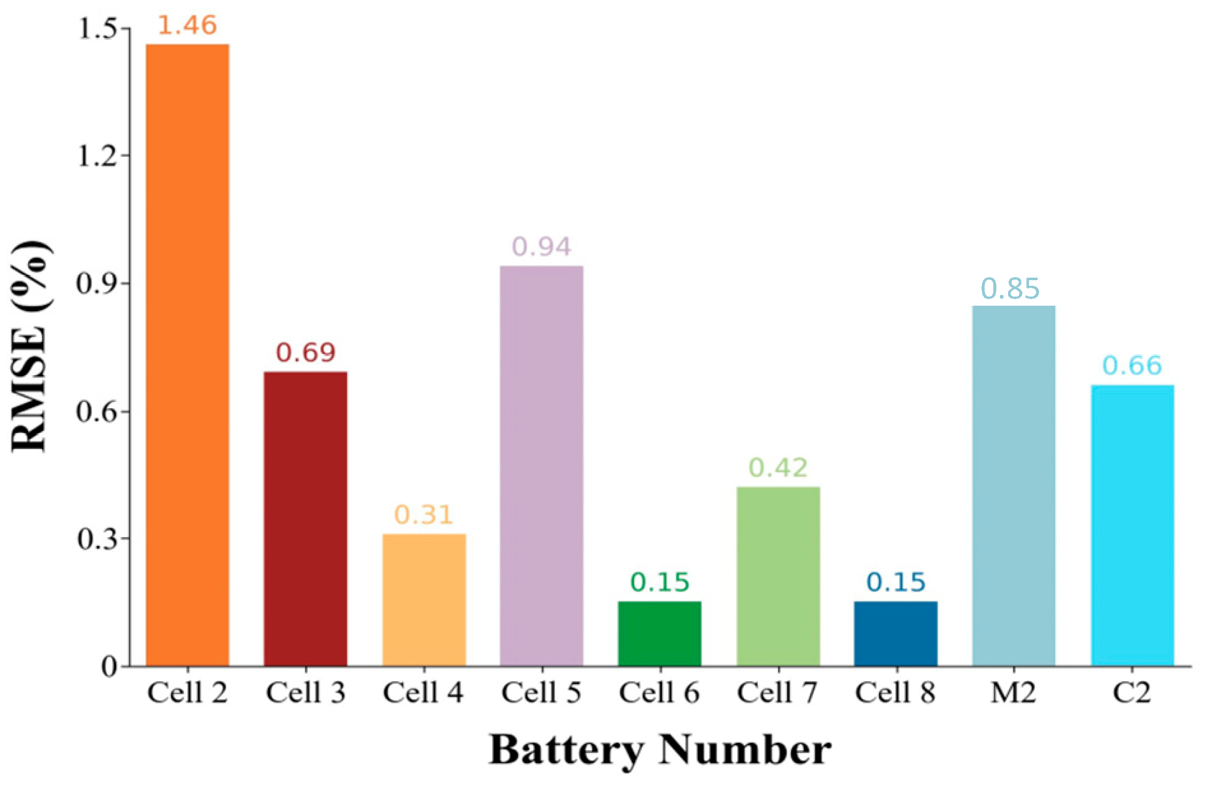
3.2. Estimated Results and Errors for Each Cell Capacity
4. Discussion
5. Conclusions
Author Contributions
Funding
Data Availability Statement
Conflicts of Interest
Nomenclature
| PEMFCs | Proton-exchange membrane fuel cells |
| SEI | Solid–electrolyte interphase |
| CNN | Convolutional neural network |
| RNN | Recurrent neural network |
| LSTM | Long short-term memory |
| TCN | Temporal convolutional network |
| BiGRU | Bidirectional gated recurrent unit |
| KOA | Kepler optimization algorithm |
| DCC | Distance correlation coefficient |
| C(k) | Capacity for the kth cycle |
| DCC of the capacity series to the i th factor | |
| Predicted probability | |
| Convolutional output | |
| True value of capacity | |
| MIT | Massachusetts Institute of Technology |
| SOH | State of health |
| RUL | Remaining useful life |
| SOC | State of charge |
| CC | Constant current |
| CV | Constant voltage |
| ICA | Incremental capacity analysis |
| HF | Health factor |
| MAE | Mean absolute error |
| RMSE | Root-mean-square error |
| MAPE | Mean absolute percentage error |
| Value of the kth cycle of the ith factor | |
| Gravitation between planets and the Sun | |
| Network output of dilation convolution | |
| Output of the residual connection | |
| Predicted capacity value |
References
- Wang, Z.; Li, M.; Zhao, F.; Ji, Y.; Han, F. Status and Prospects in Technical Standards of Hydrogen-Powered Ships for Advancing Maritime Zero-Carbon Transformation. Int. J. Hydrogen Energy 2024, 62, 925–946. [Google Scholar] [CrossRef]
- Li, X.; Ju, L.; Geng, G.; Jiang, Q. Data-Driven State-of-Health Estimation for Lithium-Ion Battery Based on Aging Features. Energy 2023, 274, 127378. [Google Scholar] [CrossRef]
- Wang, Z.; Dong, B.; Wang, Y.; Li, M.; Liu, H.; Han, F. Analysis and Evaluation of Fuel Cell Technologies for Sustainable Ship Power: Energy Efficiency and Environmental Impact. Energy Convers. Manag. X 2024, 21, 100482. [Google Scholar] [CrossRef]
- Gürbüz, H.; Akçay, H.; Demirtürk, S.; Topalcı, Ü. Techno-Enviro-Economic Comparison Analysis of a PEMFC and a Hydrogen-Fueled SI Engine. Appl. Therm. Eng. 2024, 243, 122528. [Google Scholar] [CrossRef]
- Lü, X.; Qu, Y.; Wang, Y.; Qin, C.; Liu, G. A Comprehensive Review on Hybrid Power System for PEMFC-HEV: Issues and Strategies. Energy Convers. Manag. 2018, 171, 1273–1291. [Google Scholar] [CrossRef]
- Lu, J.; Abed, A.M.; Nag, K.; Fayed, M.; Deifalla, A.; Al-Zahrani, A.; Ghamry, N.A.; Galal, A.M. Optimization of a Near-Zero-Emission Energy System for the Production of Desalinated Water and Cooling Using Waste Energy of Fuel Cells. Chemosphere 2023, 336, 139035. [Google Scholar] [CrossRef]
- Vanem, E.; Salucci, C.B.; Bakdi, A.; Alnes, Ø.Å.S. Data-Driven State of Health Modelling—A Review of State of the Art and Reflections on Applications for Maritime Battery Systems. J. Energy Storage 2021, 43, 103158. [Google Scholar] [CrossRef]
- Naseri, F.; Barbu, C.; Sarikurt, T. Optimal Sizing of Hybrid High-Energy/High-Power Battery Energy Storage Systems to Improve Battery Cycle Life and Charging Power in Electric Vehicle Applications. J. Energy Storage 2022, 55, 105768. [Google Scholar] [CrossRef]
- Xiao, Y.; Wen, J.; Yao, L.; Zheng, J.; Fang, Z.; Shen, Y. A Comprehensive Review of the Lithium-Ion Battery State of Health Prognosis Methods Combining Aging Mechanism Analysis. J. Energy Storage 2023, 65, 107347. [Google Scholar] [CrossRef]
- Tian, H.; Qin, P.; Li, K.; Zhao, Z. A Review of the State of Health for Lithium-Ion Batteries: Research Status and Suggestions. J. Clean. Prod. 2020, 261, 120813. [Google Scholar] [CrossRef]
- Ju, L.; Li, X.; Geng, G.; Jiang, Q. Degradation Diagnosis of Lithium-Ion Batteries Considering Internal Gas Evolution. J. Energy Storage 2023, 71, 108084. [Google Scholar] [CrossRef]
- Ju, L.; Long, P.; Geng, G.; Jiang, Q. Open Circuit Voltage—State of Charge Curve Calibration by Redefining Max–Min Bounds for Lithium-Ion Batteries. J. Energy Storage 2024, 79, 110224. [Google Scholar] [CrossRef]
- Yang, D.; Zhang, X.; Pan, R.; Wang, Y.; Chen, Z. A Novel Gaussian Process Regression Model for State-of-Health Estimation of Lithium-Ion Battery Using Charging Curve. J. Power Sources 2018, 384, 387–395. [Google Scholar] [CrossRef]
- Gu, X.; See, K.W.; Li, P.; Shan, K.; Wang, Y.; Zhao, L.; Lim, K.C.; Zhang, N. A Novel State-of-Health Estimation for the Lithium-Ion Battery Using a Convolutional Neural Network and Transformer Model. Energy 2023, 262, 125501. [Google Scholar] [CrossRef]
- Liu, J.; Chen, Z. Remaining Useful Life Prediction of Lithium-Ion Batteries Based on Health Indicator and Gaussian Process Regression Model. IEEE Access 2019, 7, 39474–39484. [Google Scholar] [CrossRef]
- Sun, J.; Kainz, J. State of Health Estimation for Lithium-Ion Batteries Based on Current Interrupt Method and Genetic Algorithm Optimized Back Propagation Neural Network. J. Power Sources 2024, 591, 233842. [Google Scholar] [CrossRef]
- Deng, Z.; Hu, X.; Li, P.; Lin, X.; Bian, X. Data-Driven Battery State of Health Estimation Based on Random Partial Charging Data. IEEE Trans. Power Electron. 2022, 37, 5021–5031. [Google Scholar] [CrossRef]
- Chen, L.; Bao, X.; Lopes, A.M.; Xu, C.; Wu, X.; Kong, H.; Ge, S.; Huang, J. State of Health Estimation of Lithium-Ion Batteries Based on Equivalent Circuit Model and Data-Driven Method. J. Energy Storage 2023, 73, 109195. [Google Scholar] [CrossRef]
- Liu, F.; Liu, X.; Su, W.; Lin, H.; Chen, H.; He, M. An Online State of Health Estimation Method Based on Battery Management System Monitoring Data. Int. J. Energy Res. 2020, 44, 6338–6349. [Google Scholar] [CrossRef]
- Zhou, L.; Zhang, Z.; Liu, P.; Zhao, Y.; Cui, D.; Wang, Z. Data-Driven Battery State-of-Health Estimation and Prediction Using IC Based Features and Coupled Model. J. Energy Storage 2023, 72, 108413. [Google Scholar] [CrossRef]
- Li, X.; Wang, Z.; Yan, J. Prognostic Health Condition for Lithium Battery Using the Partial Incremental Capacity and Gaussian Process Regression. J. Power Sources 2019, 421, 56–67. [Google Scholar] [CrossRef]
- Li, X.; Wang, Z.; Zhang, L.; Zou, C.; Dorrell, D.D. State-of-Health Estimation for Li-Ion Batteries by Combing the Incremental Capacity Analysis Method with Grey Relational Analysis. J. Power Sources 2019, 410–411, 106–114. [Google Scholar] [CrossRef]
- Chang, C.; Wang, Q.; Jiang, J.; Wu, T. Lithium-Ion Battery State of Health Estimation Using the Incremental Capacity and Wavelet Neural Networks with Genetic Algorithm. J. Energy Storage 2021, 38, 102570. [Google Scholar] [CrossRef]
- Tang, T.; Yang, X.; Li, M.; Li, X.; Huang, H.; Guan, C.; Huang, J.; Wang, Y.; Zhou, C. Deep Learning Model-Based Real-Time State-of-Health Estimation of Lithium-Ion Batteries under Dynamic Operating Conditions. Energy 2025, 317, 134697. [Google Scholar] [CrossRef]
- Attia, P.M.; Grover, A.; Jin, N.; Severson, K.A.; Markov, T.M.; Liao, Y.-H.; Chen, M.H.; Cheong, B.; Perkins, N.; Yang, Z.; et al. Closed-Loop Optimization of Fast-Charging Protocols for Batteries with Machine Learning. Nature 2020, 578, 397–402. [Google Scholar] [CrossRef]
- Xu, H.; Wu, L.; Xiong, S.; Li, W.; Garg, A.; Gao, L. An Improved CNN-LSTM Model-Based State-of-Health Estimation Approach for Lithium-Ion Batteries. Energy 2023, 276, 127585. [Google Scholar] [CrossRef]
- He, J.; Bian, X.; Liu, L.; Wei, Z.; Yan, F. Comparative Study of Curve Determination Methods for Incremental Capacity Analysis and State of Health Estimation of Lithium-Ion Battery. J. Energy Storage 2020, 29, 101400. [Google Scholar] [CrossRef]
- Goh, H.H.; Lan, Z.; Zhang, D.; Dai, W.; Kurniawan, T.A.; Goh, K.C. Estimation of the State of Health (SOH) of Batteries Using Discrete Curvature Feature Extraction. J. Energy Storage 2022, 50, 104646. [Google Scholar] [CrossRef]
- Xiong, R.; Sun, Y.; Wang, C.; Tian, J.; Chen, X.; Li, H.; Zhang, Q. A Data-Driven Method for Extracting Aging Features to Accurately Predict the Battery Health. Energy Storage Mater. 2023, 57, 460–470. [Google Scholar] [CrossRef]
- Abdel-Basset, M.; Mohamed, R.; Azeem, S.A.A.; Jameel, M.; Abouhawwash, M. Kepler Optimization Algorithm: A New Metaheuristic Algorithm Inspired by Kepler’s Laws of Planetary Motion. Knowl.-Based Syst. 2023, 268, 110454. [Google Scholar] [CrossRef]
- Li, L.; Li, Y.; Mao, R.; Li, L.; Hua, W.; Zhang, J. Remaining Useful Life Prediction for Lithium-Ion Batteries with a Hybrid Model Based on TCN-GRU-DNN and Dual Attention Mechanism. IEEE Trans. Transp. Electrif. 2023, 9, 4726–4740. [Google Scholar] [CrossRef]
- Zhou, G.; Guo, Z.; Sun, S.; Jin, Q. A CNN-BiGRU-AM Neural Network for AI Applications in Shale Oil Production Prediction. Appl. Energy 2023, 344, 121249. [Google Scholar] [CrossRef]
- Tang, A.; Jiang, Y.; Yu, Q.; Zhang, Z. A Hybrid Neural Network Model with Attention Mechanism for State of Health Estimation of Lithium-Ion Batteries. J. Energy Storage 2023, 68, 107734. [Google Scholar] [CrossRef]
- Chen, Z.; Zhao, H.; Zhang, Y.; Shen, S.; Shen, J.; Liu, Y. State of Health Estimation for Lithium-Ion Batteries Based on Temperature Prediction and Gated Recurrent Unit Neural Network. J. Power Sources 2022, 521, 230892. [Google Scholar] [CrossRef]
- Duan, W.; Song, S.; Xiao, F.; Chen, Y.; Peng, S.; Song, C. Battery SOH Estimation and RUL Prediction Framework Based on Variable Forgetting Factor Online Sequential Extreme Learning Machine and Particle Filter. J. Energy Storage 2023, 65, 107322. [Google Scholar] [CrossRef]
- Li, W.; Li, Y.; Garg, A.; Gao, L. Enhancing Real-Time Degradation Prediction of Lithium-Ion Battery: A Digital Twin Framework with CNN-LSTM-Attention Model. Energy 2024, 286, 129681. [Google Scholar] [CrossRef]
- Zhou, Z.; Liu, Y.; Zhao, Z.; Xia, H.; Chen, Z.; Zhang, Y. Automatic Feature Extraction-Enabled Lithium-Ion Battery Capacity Estimation Using Random Fragmented Charging Data. IEEE Trans. Transp. Electrif. 2024, 10, 8845–8856. [Google Scholar] [CrossRef]
- Tao, T.; Ji, C.; Dai, J.; Rao, J.; Wang, J.; Sun, W.; Romagnoli, J. Data-Based Health Indicator Extraction for Battery SOH Estimation via Deep Learning. J. Energy Storage 2024, 78, 109982. [Google Scholar] [CrossRef]
- Hu, X.; Che, Y.; Lin, X.; Onori, S. Battery Health Prediction Using Fusion-Based Feature Selection and Machine Learning. IEEE Trans. Transp. Electrif. 2021, 7, 382–398. [Google Scholar] [CrossRef]
- Che, Y.; Deng, Z.; Lin, X.; Hu, L.; Hu, X. Predictive Battery Health Management with Transfer Learning and Online Model Correction. IEEE Trans. Veh. Technol. 2021, 70, 1269–1277. [Google Scholar] [CrossRef]
- Wang, F.; Zhai, Z.; Zhao, Z.; Di, Y.; Chen, X. Physics-Informed Neural Network for Lithium-Ion Battery Degradation Stable Modeling and Prognosis. Nat. Commun. 2024, 15, 4332. [Google Scholar] [CrossRef]
- Zhu, J.; Wang, Y.; Huang, Y.; Bhushan Gopaluni, R.; Cao, Y.; Heere, M.; Mühlbauer, M.J.; Mereacre, L.; Dai, H.; Liu, X.; et al. Data-Driven Capacity Estimation of Commercial Lithium-Ion Batteries from Voltage Relaxation. Nat. Commun. 2022, 13, 2261. [Google Scholar] [CrossRef]
- Newman, J.; Thomas-Alyea, K.E. Electrochemical Systems; John Wiley & Sons: Hoboken, NJ, USA, 2012. [Google Scholar]


| Battery No. | First 10 Min Fast Charging Protocol | Charging Protocol After 10 Min | Discharge Protocol | (Ah) |
|---|---|---|---|---|
| M1 | 4.8 C+5.2 C+5.2 C+4.16 C | 1 C+CV | 4 C Constant Current Discharge | 1.1 |
| M2 | 7.0 C+4.8 C+4.8 C+3.65 C | 1 C+CV | 4 C Constant Current Discharge | 1.1 |
| Battery No. | Charge Protocol | Discharge Protocol | (mAh) | Testing Mode |
|---|---|---|---|---|
| Cells 1–8 | 2 C | ARTEMIS urban driving cycle | 740 | Simulation conditions |
| Cells 1–8 | 1 C | 1 C | 740 | Characteristic test |
| Parameter | Value | Parameter | Value |
|---|---|---|---|
| Rated Capacity (Ah) | 3.8 | Max. Discharge Current (A) | 15 |
| Cell Chemistry | LFP/C | Weight (g) | ≈85 |
| Voltage Range (V) | 2–3.6 | Standard Voltage (V) | 3.2 |
| Battery No. | Charge Protocol | Discharge Protocol | (Ah) | (°C) |
|---|---|---|---|---|
| C1 and C2 | 2 C-CV | Simulation of ship sailing conditions + 4 C constant-current discharge | 3.8 | 10–15 |
| Health Factors | Battery Number | ||
|---|---|---|---|
| Cell 1 | M1 | C1 | |
| Partial Charge Time (HF1) | 0.993 | 0.990 | 0.980 |
| IC Peak (HF2) | 0.917 | 0.986 | 0.939 |
| IC Peak Position (HF3) | 0.955 | / | 0.603 |
| IC Area (HF4) | 0.858 | 0.961 | 0.985 |
| Terminal Voltage after Simulation (HF5) | / | / | 0.973 |
| Method | Battery No. and Evaluation Criteria (%) | |||||||
|---|---|---|---|---|---|---|---|---|
| Cell 2 | Cell 3 | Cell 4 | Cell 5 | Cell 6 | Cell 7 | Cell 8 | M2 | |
| Proposed | MAE | MAE | MAE | MAE | MAE | MAE | MAE | MAE |
| [1.06] | [0.52] | [0.12] | [0.59] | [0.11] | [0.3] | [0.19] | [0.66] | |
| RMSE | RMSE | RMSE | RMSE | RMSE | RMSE | RMSE | RMSE | |
| [1.46] | [0.69] | [0.31] | [0.94] | [0.15] | [0.42] | [0.15] | [0.85] | |
| CNN-CBAM-LSTM [33] | MAE | MAE | MAE | MAE | MAE | MAE | / | / |
| [0.26] | [0.27] | [0.28] | [0.35] | [0.30] | [0.34] | |||
| RMSE | RMSE | RMSE | RMSE | RMSE | RMSE | |||
| [0.35] | [0.25] | [0.34] | [0.41] | [0.36] | [0.49] | |||
| GRU [34] | MAE | MAE | MAE | MAE | MAE | MAE | MAE | / |
| [1.02] | [0.66] | [0.98] | [0.62] | [0.78] | [0.51] | [0.76] | ||
| RMSE | RMSE | RMSE | RMSE | RMSE | RMSE | RMSE | ||
| [1.20] | [0.83] | [1.14] | [0.72] | [0.93] | [0.59] | [0.88] | ||
| IWOA-VFOS-ELM [35] | / | MAE [0.87] RMSE [1.15] | / | / | MAE [0.58] RMSE [0.95] | MAE [0.34] RMSE [0.44] | MAE [0.37] RMSE [0.49] | / |
| CNN-LSTM [36] | / | / | / | / | / | MAE [2.72] RMSE [1.61] | MAE [1.28] RMSE [0.78] | / |
| DAE-Bayesian NN [37] | MAE [2.19] RMSE [3.19] | MAE [0.98] RMSE [0.83] | MAE [1.75] RMSE [2.00] | MAE [2.34] RMSE [3.43] | / | / | / | / |
| BiLSTM [38] | / | / | / | / | / | / | / | MAE |
| [1.29] | ||||||||
| RVM [39] | / | / | / | / | / | / | / | MAE |
| [1.37] | ||||||||
| RMSE | ||||||||
| [3.53] | ||||||||
| TL-GRU [40] | / | / | / | / | / | / | / | MAE |
| [0.61] | ||||||||
| RMSE | ||||||||
| [0.92] | ||||||||
| PINN [41] | / | / | / | / | / | / | / | RMSE |
| [0.74] | ||||||||
| XGBoost + SVR [42] | / | / | / | / | / | / | / | RMSE |
| [1.10] | ||||||||
Disclaimer/Publisher’s Note: The statements, opinions and data contained in all publications are solely those of the individual author(s) and contributor(s) and not of MDPI and/or the editor(s). MDPI and/or the editor(s) disclaim responsibility for any injury to people or property resulting from any ideas, methods, instructions or products referred to in the content. |
© 2025 by the authors. Licensee MDPI, Basel, Switzerland. This article is an open access article distributed under the terms and conditions of the Creative Commons Attribution (CC BY) license (https://creativecommons.org/licenses/by/4.0/).
Share and Cite
Yang, X.; Tang, J.; Song, Q.; Liu, Y.; Liu, L.; Zhou, X.; Chen, Y.; Tang, T. Capacity Estimation of Lithium-Ion Battery Systems in Fuel Cell Ships Based on Deep Learning Model. J. Mar. Sci. Eng. 2025, 13, 1168. https://doi.org/10.3390/jmse13061168
Yang X, Tang J, Song Q, Liu Y, Liu L, Zhou X, Chen Y, Tang T. Capacity Estimation of Lithium-Ion Battery Systems in Fuel Cell Ships Based on Deep Learning Model. Journal of Marine Science and Engineering. 2025; 13(6):1168. https://doi.org/10.3390/jmse13061168
Chicago/Turabian StyleYang, Xiangguo, Jia Tang, Qijia Song, Yifan Liu, Lin Liu, Xingwei Zhou, Yuelin Chen, and Telu Tang. 2025. "Capacity Estimation of Lithium-Ion Battery Systems in Fuel Cell Ships Based on Deep Learning Model" Journal of Marine Science and Engineering 13, no. 6: 1168. https://doi.org/10.3390/jmse13061168
APA StyleYang, X., Tang, J., Song, Q., Liu, Y., Liu, L., Zhou, X., Chen, Y., & Tang, T. (2025). Capacity Estimation of Lithium-Ion Battery Systems in Fuel Cell Ships Based on Deep Learning Model. Journal of Marine Science and Engineering, 13(6), 1168. https://doi.org/10.3390/jmse13061168