Abstract
The accurate identification of collision positions on containers is critical in logistics and trade for enhancing cargo safety and determining accident liability. Traditional visual inspection methods are labor-intensive, time-consuming, and costly. This study leverages data from an Inertial Measurement Unit sensor and evaluates combinations of machine learning models and feature selection methods to identify the optimal approach for collision position detection. Five machine learning models (decision tree, k-nearest neighbors, support vector machine, random forest, and extreme gradient boosting) and five feature selection methods (Pearson’s correlation coefficient, mutual information, sequential forward selection, sequential backward selection, and extra trees) were assessed using three performance metrics: accuracy, execution time, and CPU utilization. Statistical analysis with the Friedman test confirmed significant differences in model and feature selection performance. The combination of k-nearest neighbors and extra trees achieved the highest accuracy of 97.1%, demonstrating that inexpensive IMU acceleration data can provide a cost-effective, efficient, and reliable solution for collision detection. This has strong practical implications for improving accident accountability and reducing inspection costs in the logistics industry.
1. Introduction
The trade and logistics industry, heavily reliant on container usage, faces significant challenges due to frequent container collisions, and these collisions are one of the primary sources of container damage [1]. Research has shown that 70% of rail and road transport vehicles have defects in container securing and packaging [2], increasing the risk of damage to containers or their contents in collision incidents. Studies have shown that improper container securing and poor cargo packaging are the main causes of damage to commercial goods [3].
Although container ships handle over 80% of international cargo transport and more than 90% of goods are transported via containers [4], a substantial body of research on containers has focused on their operation, management, and risk assessment at seaports [5,6,7,8,9,10,11]. At present, traditional methods for inspecting container damage and collision positions often require trained personnel to conduct visual inspections based on container management standards [12,13,14]. However, this approach is not only time-consuming and labor-intensive but also entails significant costs regarding training and managing inspectors, thereby compromising work efficiency and inflating inspection expenses. Research has demonstrated that human error is the primary cause of maritime accidents, with approximately 75% to 96% of such incidents attributed to human factors, including crew negligence, improper operation, and misjudgment [15]. Furthermore, the accuracy of test results is often constrained by the inspectors’ experience and subjective judgment, making it challenging to achieve standardized and consistent evaluations. To alleviate these challenges, some studies have proposed using image recognition technology to improve work efficiency and reduce management costs [16,17,18,19]. However, the image recognition method often requires the use of high-definition camera equipment, which is very expensive, and image recognition can only inspect damage on the surface of containers and lacks attention to the state of the contents within the containers.
Although physical damage is the main cause of damage to container cargo, accounting for 25% [20], certain collisions may leave the container’s surface unscathed but cause an internal impact or cargo displacement, resulting in damage. This issue is particularly important for fragile items, such as glass products, electronic components, precision instruments, and similar delicate goods. This gives rise to the following issues: (1) if the surface of the container remained intact after a collision, any damage to the goods inside could have been easily overlooked; and (2) then it is difficult to determine whether the damage to the goods was caused by a collision. Therefore, accurately identifying the collided positions in container accidents has become imperative. Identifying the collided positions could not only enhance the effectiveness of goods safety supervision but also provide a reliable basis for the determination of accident liability, holding significant theoretical and practical significance.
In this study, we made the first attempt to combine the Inertial Measurement Unit (IMU) sensor with machine learning (ML) technologies to develop a new method for detecting the collision positions of containers. This method identifies the collision positions by analyzing the high-frequency vibration data captured by the accelerometer. In contrast to traditional manual detection and image recognition methods that rely on intensive human labor and expensive equipment like high-definition cameras, our technology significantly reduces labor and equipment costs, as well as the high computational costs associated with processing high-definition image data. With a simple and cost-effective IMU sensor, we can effectively address the challenge of identifying collision positions on containers. To enhance the scalability and applicability of our method, this study integrated IMU sensor data with ML and feature selection techniques, creating an efficient, accurate, and cost-effective system for identifying collision positions in containers.
The remainder of this paper is organized as follows: Section 2 analyzes and compares existing research. Section 3 elaborates on the framework for identifying collided positions, including the processes of data collection and interpretation, the application of the feature selection (FS) method, and the ML-based detection of collided positions. Section 4 presents and explains the experiment results. Section 5 and Section 6 summarize the main findings and offer concluding remarks.
2. Related Work
Table 1 shows related research on the container collision identification problem. Traditional container damage and collision detection is carried out by manual inspection, but this method has high labor costs and low efficiency [12,13,14]. Some research has achieved automated container damage and collision inspection through image recognition methods, but this method often requires high equipment and computing costs [16,17,18,19]. Although previous studies have utilized sensors and ML to implement various container-related applications such as locating containers during transportation to ensure safety throughout the transit process [21,22,23], these studies primarily focus on the location of containers and do not address the identification of collision positions. Another study measured the fill status of liquid cargo within containers [24]; this method is applicable only to specific types of cargo and does not consider the impact of collisions on the goods. The automatic loading and transporting of containers have been explored [25]; these methods do not resolve the issue of collision detection for containers during transportation. In addition, although the detection of physical collisions between ships’ vertical sections and containers has been studied [26], this approach mainly focuses on collisions in specific scenarios and lacks a comprehensive identification of collision positions on the entire container. In the field of shipping, collision detection algorithms are used to assess the risk of collision of ships in ports and waters and to conduct a comprehensive assessment of shipping risks through data in the ship domain [27,28]. Although this type of method can also be applied to containers themselves, it mainly focuses on the assessment of collision risks between ships and lacks direct detection and analysis of container collisions.

Table 1.
Comparison of studies on container collision issues.
It was shown that FS could improve model performance, save computing re-sources, and enhance model interpretability in the field of network security attack detection [29], human activity recognition [30], medical detection [31], and contactless fault diagnosis based on the sound of a railway switch machine (RPM) [32], textual sentiment classification [33], and bridge structural health monitoring (SHM) [34]. The dataset collected from a sensor often contains high-dimensional data filled with irrelevant features and noise. Existing studies have focused solely on model performance, overlooking the computational expense incurred when processing high-dimensional data. References [35,36,37] has highlighted the issues of increased computational resource consumption and reduced model performance due to high-dimensional data. As high-dimensional data can pose significant challenges to classification algorithms [38], FS is needed. But how to effectively integrate ML and FS to identify container collision positions while reducing computational cost has not been fully explored. But how to effectively integrate ML and FS to identify container collision positions while reducing computational cost has not been fully explored.
In summary, the current body of research has faced certain challenges in accurately and cost-effectively identifying collision positions on containers, particularly when making use of sensor data. There is no research on the problem of container collision position detection using IMU sensors. There also seems to be relatively little in-depth research on the FS of high-dimensional sensor data generated by container collisions to re-duce computational overhead. As such, this study aims to address these issues by proposing a method for container collision position identification based on IMU sensor data, ML, and FS, thereby filling this gap in existing research.
3. Machine Learning-Based Identification of Collided Positions
Figure 1 shows a process flowchart of the ML-based identification of collided positions. It consists of three processes: the first process is to acquire data using the IMU sensor, the second process is to find the most helpful feature subset for detecting collided positions, and the final process is to use ML to identify collided positions.
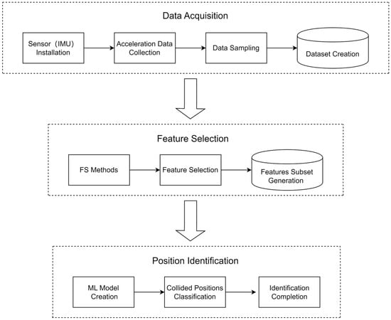
Figure 1.
Process flowchart for identifying container collided positions.
3.1. Data Acquisition
In this study, we used an IMU sensor to collect three-axis acceleration data (X, Y, Z) during collision events on a container. The IMU is a sensor mainly used to detect and measure acceleration and rotational motion. As illustrated in Figure 2, the X and Y axes of this accelerometer record horizontal data, while the Z axis records data from the vertical orientation. For the sake of data collection convenience and to simplify the installation of the sensor, this study vertically mounted it on the inside of the rear door of a container, subsequently closing the door. This arrangement allowed us to detect collisions of varying degrees in both the vertical and horizontal directions on the container, yielding three-axis acceleration data (X, Y, Z) when the container experienced a collision.
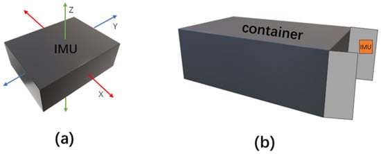
Figure 2.
(a) IMU sensor that collects (X, Y, Z) axis acceleration data. (b) Where and how to install an IMU sensor on the door of the container.
After installing the IMU sensor, this study conducted collision tests on a container in various positions, including the top, bottom, left, and right side. The sensor recorded raw acceleration data in the X, Y, and Z axes at a rate of 100 Hz. As shown in Figure 3, the time interval of each point on the horizontal axis is 10 ms, each 100 scale marks represent 1 s, the number of sampling times per second is 100 (sampling frequency: 100 Hz), and the vertical axis shows the acceleration sampling information of the X, Y, and Z axes in m/s2. The original data collected for each collision event was observed to have a very short duration, typically about a second.
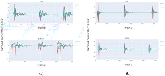
Figure 3.
Raw acceleration data collected by IMU. (a) Sampling from the top and bottom; (b) sampling from the left and right.
To avoid retaining excessive irrelevant data during the collision process, this study obtained the most pronounced samples at 30 Hz for each collision from the X-, Y-, and Z-axis acceleration data recorded by the sensor. The sample data were arranged in rows with the format [x1, y1, z1, x2, y2, z2, …, x30, y30, z30], with each row containing 90 data points, representing a single collision event. The collision events were then labeled by 0, 1, 2, and 3, corresponding to the top, bottom, left, and right positions, respectively. After labeling the column as “Class”, the entire dataset was saved in a CSV file as the original dataset.
This study obtained a dataset consisting of 661 container collision events occurring at different positions; a total of 159 collision events were recorded at the top position, 176 at the bottom, 168 at the left, and 158 at the right.
3.2. Data Description
To facilitate our understanding of the data characteristics, statistical analysis was performed on the experimental data. The dataset includes 661 collision event samples, with each sample forming a 90-dimensional feature vector by intercepting 30 consecutive three-axis accelerations (X, Y, Z axes) from the IMU sensor’s raw data sampled at 100 Hz. Table 1 presents descriptive statistics, including the mean, standard deviation, distribution patterns, and value ranges (min-max). Figure 1 and Figure 2 display the XYZ three-axis acceleration distribution histograms and feature-wise boxplots, respectively, to assist in interpreting the statistical results.
Upon examining Table 2 and Figure 4, the acceleration data across all three axes exhibit mean values close to zero and follow a normal distribution. This indicates that the measurement data are unbiased, with most values symmetrically distributed around their respective means, consistent with the characteristics of a normal distribution. Specifically, the standard deviations of the X axis (3.53) and Y axis (4.24)—representing horizontal acceleration data—are larger than that of the Z axis (3.19), suggesting that, overall, horizontal directional collision data exhibit greater volatility than vertical directional data. Within the horizontal plane, the Y axis demonstrates the highest standard deviation, implying that its collision signals are the most fluctuating and potentially more discriminative for classification tasks.
Table 2.
Descriptive statistics of accelerometer features (m/s2).
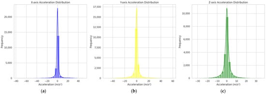
Figure 4.
X-, Y-, and Z-axis data distribution. (a) is the X-axis data distribution, (b) is the Y-axis data distribution, and (c) is the Z-axis data distribution.
Table 2 and Figure 5 further reveal that the value ranges (minimum to maximum) of the horizontal accelerations (X and Y axes) are notably larger (e.g., X axis: −77.2~50.0 m/s2), indicating drastic acceleration changes during horizontal collisions. In contrast, the Z axis (vertical acceleration) has a similarly near-zero mean but a narrower value range (−32.4~35.4 m/s2), suggesting that vertical collisions involve smaller instantaneous vibration amplitudes and correspondingly milder acceleration fluctuations. These findings highlight the distinct physical characteristics of IMU-measured accelerations during horizontal vs. vertical collisions, with the horizontal direction, on the other hand, showing a more pronounced change in dynamics.
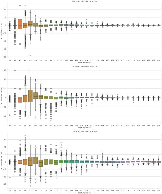
Figure 5.
The value range of each feature of the X, Y, and Z axes. (Top) represents the feature value range of the X axis, (Middle) represents the feature value range of the Y axis, and (Bottom) represents the feature value range of the Z axis.
3.3. Feature Selection
FS aims to find the optimal subset of a dataset, but finding the optimal subset of features without reducing model performance is not easy. The complete number of subsets is , where is the total number of features. Since the search time increases exponentially as increases, this study needs a more efficient FS method.
To find the most suitable FS method to reduce the data dimension for the container collision problem, we tested five representative FS techniques categorized under three mainstream approaches: two filter methods, namely Pearson’s correlation coefficient (PCC) and mutual information (MI) [39]; two wrapper methods, namely sequential forward selection (SFS) and sequential backward selection (SBS) [40]; and an embedded method, namely extra tree (ET) [41]. These five methods are logically simple, easy to implement, and fit the purpose of this study. They are suitable examples of effective feature reduction.
Figure 6 illustrates typical workflows for three main categories of FS methods: filter, wrapper, and embedded. Filter methods generally involve computing statistical measures or correlations for all features and then ranking and selecting the top-scoring subset. For instance, this study adopts PCC and MI; PCC evaluates the linear correlation between variables, whereas MI measures the amount of shared information from an information-theoretical perspective, emphasizing how strongly a feature and the target depend on each other.
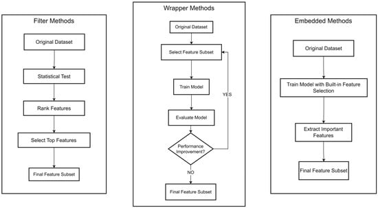
Figure 6.
The typical workflows of three main categories of FS methods.
The formula for PCC between two variables and with data points is shown in Equation (1).
where and are the means of and , respectively, and and are individual data points. PCC evaluates the linear correlation between variables.
MI, on the other hand, measures the amount of shared information from an information-theoretical perspective, emphasizing how strongly a feature and the target depend on each other. The formula for MI between two discrete random variables and is shown in Equation (2).
where and are the sample spaces of and , is the joint probability mass function of and , and and are the marginal probability mass functions of and , respectively.
When using these two methods for FS, the statistical measure score of each feature is calculated, and then the features are sorted according to the score of each feature, and finally, the top-ranked features are filtered out according to the sorting and the predetermined threshold. When using PCC and MI for FS in this study, this study first calculated the statistical scores of PCC and MI for each feature, then sorted them according to the scores and set a threshold to filter features from the sorting. The threshold is usually between 0 and 1. For example, selecting features with PCC > 0.2 means selecting features with scores exceeding 0.2 from the sorting.
Wrapper methods require setting up an ML model to train on different feature combinations and assess their performance. Based on the results, features are either added or removed to find the optimal subset. This study leverages SFS and SBS, where SFS starts from an empty set and adds the feature that most improves model performance until no further gains are observed, and SBS begins with the complete set and removes the least influential feature at each step until further removal causes a significant drop in performance.
Finally, embedded methods integrate FS into the model’s training phase itself. ET is an example, where the algorithm computes feature importance internally during training, automatically weighing each feature based on its contribution. It does this through a multitude of randomized decision trees, wherein each tree considers a random subset of features and split nodes based on the best split among a random set of features. The frequency and the context of a feature’s usage in these trees are indicative of its importance, effectively enabling the model to weigh each feature’s contribution to the prediction accuracy automatically. Compared with filter methods, embedded approaches can better account for interactions among features; compared with wrapper methods, they eliminate the need to repeatedly build and test multiple feature subsets, thus saving substantial computation.
3.4. Classification Models
Aiming to achieve precise collision detection, this study tested ML models to identify the collided positions on a container, such as decision tree (DT) [42], which is a classification algorithm based on a tree-like structure that makes decisions by recursively splitting the dataset; k-nearest neighbors (KNN) [43], which is a distance-based classification algorithm that classifies data points based on the majority class of their nearest neighbors; support vector machine (SVM) [44], which seeks to find a decision boundary that maximizes the margin between classes and is effective in handling complex and high-dimensional data; random forest (RF) [45], which is an ensemble learning algorithm that combines multiple decision trees to improve classification performance and reduce overfitting risk; and extreme gradient boosting (XGBoost) [46], which is a gradient boosting algorithm that iteratively trains weak classifiers to enhance performance.
In this study, we constructed classification models using Python version 3.11.13 along with the scikit-learn library (version 1.6.1) for the DT, KNN, SV, and RF models. The XGBoost model was implemented using the dedicated XGBoost library (version 2.1.4). Table 3 shows the parameter settings of these five models.
Table 3.
Parameter settings of ML models.
Given the limited dataset size and the high classification accuracy achieved in subsequent experiments, simplified parameter settings proved sufficient. This approach ensured robust performance without unnecessary computation, aligning with our research goal of high-efficiency computing. Consequently, no additional hyperparameter optimization techniques (e.g., grid search or Bayesian optimization) were employed. Specifically, DT and KNN, being inherently simpler models, utilized scikit-learn’s default parameters. For SVM, the radial basis function (RBF) kernel (kernel = ‘rbf’) was adopted to enhance its capability in handling non-linear decision boundaries. The RF model was configured with n_estimators = 100 and max_depth = None, a conventional setup balancing model complexity and generalization. Regarding the XGBoost model, critical parameters were explicitly defined to align with the multi-class classification task: objective = ‘multi:softmax’ specifies the multi-class classification objective; num_class = 4 indicates the four target collision position categories; and eval_metric = ‘mlogloss’ ensures proper evaluation of multi-class logarithmic loss.
3.5. Performance Verification and Overfitting
Considering the small amount of data (661 samples), this study use ten-fold cross-validation (CV) as the core validation strategy to ensure the robustness of the model evaluation. This method divides the dataset into 10 subsets in a stratified manner, with each subset maintaining the original category distribution (top: 159 samples; bottom: 176 samples; left: 168 samples; right: 158 samples). In each iteration, nine subsets are used for training, and the remaining subset is used as a validation set. This process is repeated 10 times, ensuring each sample participates in nine training and one validation iteration. Finally, the average of the 10 validations is taken as the final model performance evaluation result.
By evaluating the model on multiple different training and validation sets, data utilization is maximized, and the random fluctuations caused by the small amount of data and overfitting on a specific dataset are effectively reduced. The advantage of this method is that it integrates model validation, generalization ability evaluation, and computing resource optimization into a unified framework without the need for separate data augmentation or regularization techniques. In a small dataset of 661 samples, a ten-fold CV is equivalent to expanding the effective sample size by 9 times through full-sample loop training. Compared with some data augmentation techniques (which require the artificial generation of virtual samples and may introduce bias), CV directly utilizes the diversity of real data, avoids potential differences between the generated data and the real distribution, and more reliably improves the generalization ability of the model.
3.6. Classification Systems
To design the most effective system for identifying container collided positions, this study not only evaluated all possible combinations of FS methods and ML models but also compared two systems: a single multi-class classification system that identifies one of the four collided positions (top, bottom, left, or right) and four separate binary classification systems, each dedicated to identifying whether a collision occurred at a specific position (top, bottom, left, or right).
4. Experimental Results
In this study, we used three indicators to evaluate the classification systems: accuracy, execution time, and CPU utilization. Accuracy refers to the ratio of correctly classified samples to the total number of samples. Execution time refers to the total time taken by the model from training to evaluation through 10-fold cross-validation. CPU utilization refers to the proportion of CPU resources consumed during the model’s execution. This study carried out the experiments on a computer equipped with an Intel(R) Core (TM) i5-12400F processor, 32.0 GB of memory, an NVIDIA GeForce RTX 4060 GPU, and 1 TB of SSD storage, running the Windows 10 operating system.
4.1. Results for a Single Multi-Class Classification System
Based on the principle of the FS method shown in Figure 6, to select the optimal subset of features, this study sets the parameter settings for each FS method as follows: The filtering threshold of PCC and MI is set to 0.2, based on the analysis in Appendix A.1, to avoid too much degradation of model performance and the appearance of empty sets in feature subsets. As the classifier model for SFS and SBS, we utilized the Gaussian Naive Bayes (GaussianNB) model [47], using accuracy as the performance metric for evaluating model subsets. This choice was made due to its low computational resource requirements, aligning with our goal of minimizing computational costs. We configured the parameters for ET using the default initialization settings in the sklearn library to avoid unnecessary complexity. Before performing FS operations and implementing the ML model for classification, the dataset was standardized to eliminate the impact of different feature dimensions. This standardization helps ensure that the subsequent FS methods and ML model calculations are more effective, and it can also accelerate the convergence of the model during training.
Figure 7 shows the number of features selected by each FS method. All FS methods effectively reduced the feature dimension compared with the original data. Compared to the original data, even the MI method, which selects the largest number of features, only selected 23 features out of the original 90 features from the XYZ-axis acceleration sampling data, while the SFS method selects the least number of features from the 90 original data features, only 9. ET selects 11 features, the second smallest number of features. PCC selects 15 features, the third smallest number of features, followed by SBS, which selects 19 features, the fourth smallest number of features, only 4 features less than MI, which selects the largest number of features.
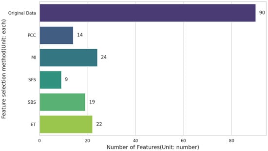
Figure 7.
Number of features selected by different FS methods.
This study evaluated the accuracies of the five ML models using the features selected by the five FS methods, respectively. Table 4 shows the results, including those obtained from using the original data. From the table, we can see that all FS methods show a similar level of accuracy as the original data. The accuracy of some FS methods is even better than that of the original data. For example, the accuracy of DT using 90 features from the original data is 93%, while it is 94.4% for the SFS method with only 9 features. The accuracy of KNN using 90 features from the original data is 92.9%, while this is improved to 97.1% for the ET method with 11 features. The accuracy of SVM using 90 features from the original data is 94.9%, while this is improved to 97.1% for the SBS method with 19 features.
Table 4.
Accuracy of different FS methods and ML models.
Comparing all the accuracies of the ML model and FS method combinations, the best-performing combination is XGBoost and SBS. This combination achieved an accuracy of 98.5%. Although this result was the same as that obtained using the original data, the number of features was reduced from 90 to 19, which is a significant reduction in feature dimensionality. This result is enough to show that from the perspective of saving computing resources, the combination of XGBoost and SBS is better than using XGBoost alone to classify the original 90 acceleration data features.
Table A2 and Table A3 show the execution time and CPU utilization of each ML model for different FS methods. We can see that FS has a significant effect on reducing time and CPU utilization. For example, the time taken by RF for the original data is up to 2.392 s, while the time taken by RF using the features selected by ET is reduced to 1.099 s. The CPU utilization of XGBoost for the original data is up to 25.40%, while it is reduced to 14.75% when using SFS. Among all the combinations, the combination that takes the least time is KNN and SFS, which takes only 0.029 s. In terms of CPU utilization, the combination of KNN and ET is relatively good, consuming only 0.10% of CPU.
Looking at the results, we found that the combinations with the best performance in terms of accuracy, execution time, and CPU utilization are different. By observing the values of the three indicators, we determined the following two criteria for evaluating the best model:
(1) The minimum accuracy must be maintained above 95%.
(2) Models with high accuracy, low execution time, and low CPU utilization should be chosen as much as possible.
According to the above two evaluation criteria, selecting the combination of ML and FS can balance the relationship between accuracy and efficiency, thus helping us find the best combination of ML and FS with both accuracy and efficiency. So according to the criteria, the best combination is KNN and ET. The accuracy of this combination is 97.1%, which exceeds the criterion of 95%. Although the accuracy is not the highest, it has the lowest execution time and CPU utilization of 0.300 s and 0.10%, respectively. Compared with the results of other models, such as RF and XBboost, under the premise of using ET as the FS method, although they obtained higher accuracies of 98.0% and 98.3%, respectively, their execution time and CPU utilization were also higher. Taking the RF model as an example, its execution time is 1.099 s and CPU utilization is 1.65%, which is higher than the best combination of KNN and ET that we selected.
4.2. Results for Separate Binary Classification Systems
To explore the best way to identify container collision positions, in this experiment, we also evaluated the four binary classification systems where each selected class, such as top, bottom, left, or right, is distinguished from all other classes. The selected class is labeled as positive (1), and all other classes are combined as negative (0). Figure 8 shows the number of features selected by the five FS methods for each classification system. In this study, we call each classification system Class 0, Class 1, Class 2, and Class 3 according to the top, bottom, left, and right positions, respectively. Specifically, the minimum number of features for Class 0 is given by MI, which is only 1, while those for Class 1, Class 2, and Class 3 are given by SFS, which are 3, 4, and 2, respectively, in contrast to Figure 8, where the minimum number of features was 9 for SFS. The binary classification systems can reduce the feature dimensions more significantly, obtaining a smaller subset of features.
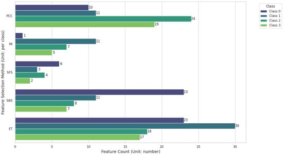
Figure 8.
Histogram of the number of features selected by different FS methods for different categories.
Table 5, Table A4 and Table A5 show the accuracy, execution time, and CPU utilization for Class 0. Based on the criteria we set before, the best combination is KNN and PCC. First, its accuracy of 95.8% is higher than the criterion of 95%. Secondly, the execution time, 0.310 s, is the least among all the combinations with an accuracy greater than 95%. Finally, the CPU utilization is 0.20%, the minimum among all the combinations.
Table 5.
Accuracy (%) of different FS methods and ML models on Class 0 data.
Table 6, Table A6 and Table A7 show the accuracy, execution time, and CPU utilization for Class 1. Overall, KNN and SBS form the best combination, with an accuracy of 97.9%, an execution time of 0.03 s, and a CPU utilization of 0.15%. The accuracy is higher than the criterion of 95%. Although the execution time is greater than that of the KNN and SFS combination, the accuracy is higher. Furthermore, the CPU utilization is the least, only 0.15%.
Table 6.
Accuracy (%) of different FS methods and ML models on Class 1 data.
Table 7, Table A8 and Table A9 show the accuracy, execution time, and CPU utilization for Class 2. The best combination is DT and SFS. Its accuracy is 99.1%, which is higher than the criterion of 95%. In addition, it has the lowest execution time and CPU utilization, only 0.013 s and 0.25%, respectively.
Table 7.
Accuracy (%) of different FS methods and ML models on Class 2 data.
Table 8, Table A10 and Table A11 show accuracy, execution time, and CPU utilization for Class 3. The best combination is DT and ET, with an accuracy of 98.0%, which is above the criterion of 95%. In terms of execution time, although the execution time of DT+MI, DT+SFS, and DT+SBS are better than DT+ET’s 0.018 s, which are 0.013 s, 0.011 s, and 0.015 s respectively, their accuracy rates are 97.7%, 95.6%, and 97.0%, respectively, which are lower than DT+ET’s 98.0%. Furthermore, the combination of DT and ET has the lowest CPU utilization, only 0.10%.
Table 8.
Accuracy (%) of different FS methods and ML models on Class 3 data.
Table 9 summarizes the best combination for each classification system and its performance. We can see that the performances are different from each other. The best performance is seen for Class 2, with the highest accuracy of 99.1%, the lowest execution time of 0.013 s, and the lowest CPU utilization of 0.05%, respectively. The performance of Class 0 is the lowest, with an accuracy of 95.8%, an execution time of 0.031 s, and a CPU utilization of 0.20%, respectively. When comparing this with the best performance of the single multi-class classification system (accuracy 97.1%, execution time 0.300 s, and CPU utilization 0.10%), we know that using the single multi-class classification system produces more stable results than using a different binary classification system according to the target position.
Table 9.
Best combinations and their performances.
Figure 9 shows the accuracy heat map for the four classes. The vertical axis represents the ML model, and the horizontal axis represents the FS method. Each number is the accuracy of the corresponding combination; the closer the color is to yellow, the higher the accuracy, and the closer the color is to blue, the lower the accuracy. We see that the overall color for Class 2 is closest to yellow, followed by Class 3 and Class 1. In contrast, Class 0 shows that the overall color is closest to dark green. This indicates that all combinations for Class 0 exhibit relatively poor performance. According to Table 5, the combination with the worst classification performance for Class 0 is DT and MI, with an accuracy of 80.2%, while the worst performances for Class 1, Class 2, and Class 3 do not fall below an accuracy of 94.0%.
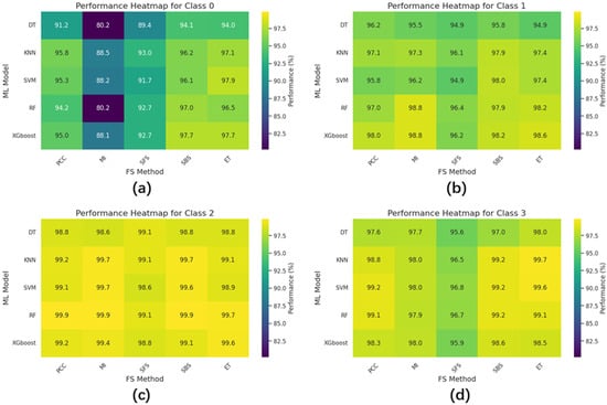
Figure 9.
Classification accuracy heat maps of the 4 separate binary classification systems. (a) is the accuracy of Class 0 data, (b) is the accuracy of Class 1 data, (c) is the accuracy of Class 2 data, and (d) is the accuracy of Class 3 data.
Figure 10 shows the distribution of the data for the four class systems after applying two-dimensional Principal Component Analysis (PCA) [48]. We found that the data distribution for Class 0 is not particularly concentrated compared with the other classes, which is the reason why the classification performance of Class 0 is poor. Collisions at different positions will produce different distributions of data. During data collection, collisions were conducted at different positions on the container. When collisions occurred, the container usually underwent a slight offset along the direction of the collision, so the data generated will be distributed more concentratedly along the collision direction, making it easier for the ML model to identify and classify. For example, in Figure 10, Class 2 and Class 3 represent the data distributions for the left and right positions, respectively. Their data distributions are relatively concentrated. Class 2, even for the worst combination of DT and MI, achieved an accuracy 98.6%, while for the best combination of RF and PCC, it achieved an accuracy 99.9%.
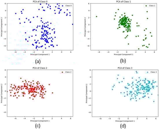
Figure 10.
Data distribution after PCA dimensionality reduction for each category of data. (a) is the distribution of Cass 0 data, (b) is the distribution of Class 1 data, (c) is the distribution of Class 2 data, and (d) is the distribution of Class 3 data.
In contrast, when the collision occurs at the top position of the container, a dis-placement caused by the collision is less likely to occur since the container is usually placed on the ground. The container can only vibrate at its original position, producing data that is more widely distributed than for the other positions and correspondingly more difficult to classify. As we can see from the results in Table 7 and Figure 9, the performance for Class 2 is high, which means that Class 2 is easier to classify, while the performance for Class 0 is low, which means that Class 0 is the most difficult to classify. This shows that the container collision data collected by sensor data have different properties.
In conclusion, the results show that it is more reasonable to use the single multi-class classification system with a combination of KNN and ET than separate binary classification systems. Compared with a single multi-class classification system, the performances of separate binary classification systems varies greatly among different categories. Therefore, using a single multi-class classification system is the most stable option and produces the best performance. Appendix A.3 shows the feature changes after FS. The results show that FS can effectively preserve the feature properties and facilitate the efficient training of model classification. Appendix A.4 shows the precision, recall, and F1 score of the single multi-class classification system. The results show that our best selected classification systems, KNN and ET, have stable performance. Furthermore, one system is operationally simpler since separate systems demand a lot of additional workloads and a more complicated workflow.
4.3. Statistical Analysis of Results for Best Classification System
To verify the credibility of the classification system results constructed by our optimal combination of KNN + ET, we employed the Friedman test from three perspectives—accuracy, execution time, and CPU utilization—to statistically analyze the performance of different models (DT, KNN, SVM, RF, XGBoost) and different FS methods (PCC, MI, SFS, SBS, ET). The Friedman test is a non-parametric test that is suitable when the data is repeatedly measured [49], that is, the same group of subjects is measured multiple times at different points in time or under different conditions. It is often used to compare differences between three or more matched groups. The reason for choosing the Friedman test is that, in this study, each ML model or FS method is evaluated under multiple conditions of the other factor. In addition, our sample size is relatively small, and multiple treatment groups (≥3 groups) need to be compared simultaneously. The Friedman test is a non-parametric alternative to repeated-measures ANOVA that meets the requirements of our research.
In this study, the statistical analysis focused on exploring the following performance results:
(1) Whether there is a statistically significant difference in the performance of the five models under different FS methods.
(2) Whether there is a statistically significant difference in the performance of the five FS methods under different models.
Table 4, Table A2 and Table A3 contain the accuracy, execution time, and CPU utilization results of the five models (rows) under the five FS methods (columns) and the original dataset characteristics, respectively, forming a 5 × 6 data matrix, which also includes the performance of our best combination KNN + ET. These performance results are all derived from the same dataset, ensuring that each model–FS combination was tested under consistent conditions. In this study, when considering the ML model as the factor, each model is evaluated using the five FS methods plus the original dataset features (paired measurements). When considering the FS method as the factor, each FS method plus the original dataset features is evaluated under five models (paired measurements). This study used Python with the pandas library (version 2.2.2) for data processing and the scipy.stats module (version 1.15.3) for statistical testing to implement the Friedman test. The data were initially stored in a wide format (Model × FS Method) and then converted to a long format for grouping analysis. We conducted two separate Friedman tests to evaluate differences at both the model level and the FS method level, employing a χ2 statistic for each test. We used a significance level (α) of 0.05 to determine statistical significance, where results with p < 0.05 were considered statistically significant. In this study, H0 and H1 are used to represent the null hypothesis and alternative hypothesis, respectively, in the statistical analysis process.
Based on the accuracy shown in Table 4, we performed two separate Friedman tests, using the models’ accuracy results as the treatment group’s H0 and H1:
H0.
Under the original dataset features plus the five FS methods, there is no significant difference in accuracy among the five models (DT, KNN, SVM, RF, XGBoost).
H1.
There is a significant difference in accuracy among the five models.
First, for the model-level Friedman test (grouped by model), the test statistic χ2 = 21.2773 and p = 0.000279 (rounded). Because p < 0.05, we reject H0, indicating that there is a statistically significant difference in the accuracy of the five models under the six FS methods. In other words, at least one model exhibits performance that differs from the other models by more than random error can explain. From the observed results, more complex models (such as RF and XGBoost) consistently show higher accuracy than simpler models (such as DT and KNN).
Using FS methods as the treatment group’s H0 and H1:
H0:
Under the five models, there is no significant difference in accuracy between the original dataset features and the five FS methods (PCC, MI, SFS, SBS, ET).
H1:
There is a significant difference in accuracy between the original dataset features and the five FS methods.
Next, for the FS method-level Friedman test (grouped by FS method), the test statistic χ2 = 6.5294 and p = 0.2581. Because p > 0.05, we fail to reject H0, indicating that there is no statistically significant difference in the accuracy between the original dataset features and the five FS methods under the five models. Although numerical differences exist (e.g., MI vs. original), these differences did not reach statistical significance with the current dataset and sample size. From a practical perspective, this demonstrates that using FS methods can indeed reduce the original dataset features without affecting the model’s accuracy.
In summary, combined with the contents of parts Appendix B.1 and Appendix B.2, although complex models (e.g., XGBoost) may improve accuracy, they also substantially increase execution time and CPU utilization. Thus, selecting an appropriate model requires consideration of computing resource limitation constraints. Meanwhile, FS methods (e.g., PCC, ET) can significantly lower CPU consumption by reducing feature dimensionality. This aligns with our previously identified optimal model combination, indicating that KNN combined with ET also meets the criteria of being the best system from a statistical standpoint.
5. Discussion
5.1. Analysis and Discussion
In this study, we successfully collected acceleration data through an IMU sensor and applied FS and ML techniques to accurately identify the collided position of the container. Compared with traditional manual detection [12,13,14] and image recognition methods [16,17,18,19], this approach offers three distinct advantages: first, the sensor can capture the collision data obtained by the IMU sensor in real time, overcoming the time and space limitations of manual detection; second, the ML model automatically identifies the collision position based on the data collected by the IMU sensor, reducing errors caused by inspectors’ experience and subjective judgment, thereby achieving more standardized recognition results; and finally, the method of using only one IMU sensor to collect data and applying ML for recognition is undoubtedly cheaper than both manual detection and image recognition. In addition, existing methods rely heavily on manual inspection or high-cost equipment, while this study directly uses IMU raw acceleration data without presetting independent variables. The advantage of this is that it simplifies the system workflow and omits unnecessary complex operations. It can automatically capture the physical characteristics of the collision position through ML using only the simplest data and realize the identification of container collision positions. Traditional manual visual inspection and image recognition rely on visible damage features on the surface of the container (such as dents and scratches) but cannot detect collisions that damage the internal cargo without causing damage to the surface. The high-frequency sampling of raw data without independent variables retains the transient details of the collision and allows us to accurately identify collisions without damage to the surface, which is impossible with traditional manual visual inspection and image recognition. Using IMU raw acceleration data without independent variables, combined with FS to remove redundant dimensions, reduces computational costs and retains key information, providing a new paradigm for low-cost, high-accuracy collision detection.
This study also discusses the difference between using a single multi-class classification system and separate binary classification systems for each collision position. It also analyzes the impact of the physical properties of the collision position on classification performance. The results show that the combination of KNN and ET achieves 97.1% accuracy, with an execution time of 0.030 s and a CPU utilization of only 0.10%. The combination of KNN and ET for the selected features achieves the best balance between accuracy, execution time, and CPU Utilization usage. Therefore, using KNN and ET to build a single multi-class classification system is the best choice. To verify the reliability of the performance of the best classification system, we use the Friedman test method and rigorous statistical analysis. We prove that KNN and ET meet the dual criteria of high performance and low computational overhead. This statistical analysis underscores the importance of balanced models and provides strong support for our findings, ensuring our classification system is both effective and efficient. The single multi-class system with the KNN and ET combination proved to be more stable and efficient, both in terms of performance and operational simplicity. This is particularly advantageous in real-world applications, where implementing multiple systems may not be feasible due to additional workload and complexity.
The contribution of this study lies in the development of an efficient solution for container collision position identification using ML and FS methods based on IMU sensor data. This balance of performance and efficiency is particularly critical for real-world deployment in resource-constrained smart containers. This study’s unique contributions include the following: (1) Only a simple and cheap IMU sensor was used to achieve low-cost container collision position detection. (2) Through comparative analysis, the best system for container collision position detection was selected. (3) It provided physical insights into collision dynamics (e.g., top collisions produce scattered IMU sensor data due to constrained container movement). (4) It enabled the efficient optimization of computing resources. Compared to traditional identification methods, this approach is not only more cost-effective but also significantly enhances efficiency, thereby improving the overall operational performance of the trade and logistics industry. By accurately identifying collision positions, this method can greatly enhance cargo safety supervision, streamline logistics operations, and reduce reliance on human labor. Furthermore, it provides reliable evidence for determining accident liability, which is critical for minimizing container and cargo losses as well as reducing claims and associated costs. The proposed system offers actionable benefits to logistics stakeholders, including reduced manual inspections, faster accident response, and data-driven liability determination.
5.2. Limitations and Future Directions
This study relies on a relatively small dataset collected under controlled conditions, which may limit the generalizability of the results. The dataset lacks changes in cargo type (e.g., solid and liquid), mode of transportation (e.g., distinction between sea and land transport), and environmental factors (e.g., weather, wind, and the navigation status of the cargo ship). These variables may change the acceleration pattern during the collision, which may reduce the robustness of the model in real-world scenarios. In addition, there are certain limitations in terms of sensor installation location and data collection. For example, does installing the IMU sensor at different locations on the container door have different effects on data collection in the above situations? In terms of practical applications, this study does not consider background noise from complex operating environments in actual logistics activities (e.g., container loading and unloading, engine vibration), which may introduce false alarms or mask collision signals. Robust testing under noisy conditions is essential for actual deployment.
To overcome these limitations, future research should expand the diversity of datasets, collect container data with different types of goods and transportation conditions, and consider different types of sensors such as accelerometers, gyroscopes, and sound sensors so that it can meet more complex and diverse scenarios. It is hoped that by making up for these shortcomings, the proposed method can be developed into a scalable, multi-scenario applicable solution for the safe transportation of smart containers, thereby further promoting the intelligent transformation and development of logistics and trade.
6. Conclusions
This study developed a system that will, for the first time, utilize acceleration data collected by IMU sensors and apply FS and ML to identify the collided position of containers accurately and efficiently with reduced costs. This system offers an optimal solution for applications with limited computing resources or where cost-saving is a priority, such as a mobile device like a smart container. This study not only boosted computing efficiency but also provided new technical support for safe transportation in the logistics industry, where containers are the primary mode of transportation.
This study has limitations that point to directions for future research. The relatively small dataset and controlled experimental conditions without cargo may limit the generalizability of the results. In practical scenarios, containers carry various types of cargo that can affect the IMU sensor’s readings during collisions. Future work should involve collecting more extensive and diverse datasets under different loading conditions and environmental factors to validate and enhance the proposed methods.
In summary, this study demonstrates that integrating an IMU sensor and ML models with FS is an effective strategy for collision position identification on containers. This approach not only enhances computational efficiency and reduces usage costs but also has the potential to significantly improve safety and operational efficiency in the logistics and trade industries.
Author Contributions
Conceptualization by X.Z., Z.S. and B.-K.P.; methodology development by X.Z., Z.S. and B.-K.P.; software implementation by X.Z.; validation by X.Z. and B.-K.P.; formal analysis by X.Z.; investigation, X.Z., Z.S., D.-M.P. and B.-K.P.; resources, D.-M.P. and B.-K.P.; data curation by X.Z.; draft by X.Z. and Z.S.; review and editing by X.Z., Z.S. and B.-K.P.; supervision by B.-K.P.; project administration by D.-M.P. and B.-K.P.; funding acquisition by D.-M.P. All authors have read and agreed to the published version of the manuscript.
Funding
This work was supported by the Dong-A University research fund.
Data Availability Statement
The data presented in this study are available on request from the corresponding author.
Conflicts of Interest
The authors declare no conflicts of interest.
Appendix A
Appendix A.1. Parameter Selection for FS Method
In this study, the threshold of PCC and MI was set to 0.2, and the results were determined by empirical validation on our dataset. Table A1 shows accuracy with a PCC threshold of 0.3. The experiments show that when the threshold is 0.3, three features are selected but the performance drops by more than 10%. When MI is set to 0.3, the feature subset is empty, which makes the model unable to train. When the threshold is 0.2, a certain number of features can be retained to avoid the subset being empty. For example, in Figure 6, for class 0 data, the MI method only selected one feature. Considering the performance and feasibility of model training, the thresholds of PCC and MI are set to 0.2. In addition, wrapper methods (SFS/SBS) and the embedded method (Extra Tree, ET) can automatically select a fixed number of feature subsets, so no additional operations are required.
Table A1.
Accuracy of each ML model when the PCC threshold is 0.3.
Table A1.
Accuracy of each ML model when the PCC threshold is 0.3.
| Model | Accuracy |
|---|---|
| Decision Tree | 81.1 |
| KNN | 83.7 |
| SVM | 82.4 |
| R F | 85.8 |
| XGBoost | 85.0 |
Appendix A.2. Execution Time and CPU Utilization Results for a Single Multi-Class Classification System
Table A2 and Table A3 present the results of a single multi-class classification system, including execution time and CPU utilization for classifying raw data and each FS data with ML models.
Table A2.
Execution time (s) for classifying raw data and each FS data with ML models.
Table A2.
Execution time (s) for classifying raw data and each FS data with ML models.
| Model | Original | PCC | MI | SFS | SBS | ET |
|---|---|---|---|---|---|---|
| DT | 0.241 | 0.048 | 0.069 | 0.031 | 0.058 | 0.035 |
| KNN | 0.133 | 0.035 | 0.034 | 0.029 | 0.034 | 0.030 |
| SVM | 0.699 | 0.281 | 0.276 | 0.195 | 0.235 | 0.164 |
| RF | 2.392 | 1.178 | 1.314 | 1.137 | 1.302 | 1.099 |
| XGBoost | 1.966 | 0.751 | 0.797 | 0.674 | 0.751 | 0.624 |
Table A3.
CPU utilization (%) for classifying raw data and each FS data with ML models.
Table A3.
CPU utilization (%) for classifying raw data and each FS data with ML models.
| Model | Original | PCC | MI | SFS | SBS | ET |
|---|---|---|---|---|---|---|
| DT | 4.45 | 0.25 | 0.50 | 0.50 | 0.20 | 0.25 |
| KNN | 1.20 | 0.50 | 1.05 | 0.35 | 1.05 | 0.10 |
| SVM | 1.25 | 0.50 | 0.80 | 0.45 | 0.60 | 3.40 |
| RF | 2.45 | 1.65 | 1.80 | 1.70 | 1.90 | 1.65 |
| XGBoost | 25.40 | 15.55 | 16.55 | 14.75 | 15.80 | 14.35 |
Table A4.
Execution time (s) of different FS methods and ML models on Class 0 data.
Table A4.
Execution time (s) of different FS methods and ML models on Class 0 data.
| Model | PCC | MI | SFS | SBS | ET |
|---|---|---|---|---|---|
| DT | 0.035 | 0.013 | 0.030 | 0.060 | 0.034 |
| KNN | 0.031 | 0.023 | 0.027 | 0.034 | 0.032 |
| SVM | 0.146 | 0.167 | 0.140 | 0.174 | 0.127 |
| RF | 1.126 | 0.763 | 0.981 | 1.282 | 1.047 |
| XGBoost | 0.240 | 0.217 | 0.230 | 0.291 | 0.219 |
Table A5.
CPU utilization (%) of different FS methods and ML models on Class 0 data.
Table A5.
CPU utilization (%) of different FS methods and ML models on Class 0 data.
| Model | PCC | MI | SFS | SBS | ET |
|---|---|---|---|---|---|
| DT | 0.45 | 0.20 | 0.30 | 0.45 | 0.25 |
| KNN | 0.20 | 0.45 | 0.15 | 0.85 | 0.20 |
| SVM | 0.40 | 0.90 | 0.50 | 0.45 | 0.40 |
| RF | 1.70 | 1.40 | 1.70 | 1.85 | 1.75 |
| XGBoost | 7.75 | 6.95 | 7.80 | 8.50 | 7.45 |
Table A6.
Execution time (s) of different FS methods and ML models on Class 1 data.
Table A6.
Execution time (s) of different FS methods and ML models on Class 1 data.
| Model | PCC | MI | SFS | SBS | ET |
|---|---|---|---|---|---|
| DT | 0.031 | 0.055 | 0.016 | 0.035 | 0.048 |
| KNN | 0.031 | 0.031 | 0.025 | 0.030 | 0.032 |
| SVM | 0.164 | 0.129 | 0.086 | 0.102 | 0.144 |
| RF | 1.071 | 1.108 | 0.705 | 1.004 | 1.102 |
| XGBoost | 0.202 | 0.188 | 0.182 | 0.189 | 0.196 |
Table A7.
CPU utilization (%) of different FS methods and ML models on Class 1 data.
Table A7.
CPU utilization (%) of different FS methods and ML models on Class 1 data.
| Model | PCC | MI | SFS | SBS | ET |
|---|---|---|---|---|---|
| DT | 0.35 | 0.30 | 0.30 | 0.30 | 0.20 |
| KNN | 0.25 | 0.30 | 0.30 | 0.15 | 0.40 |
| SVM | 0.40 | 0.40 | 0.25 | 0.50 | 0.50 |
| RF | 1.70 | 1.90 | 1.30 | 1.60 | 1.65 |
| XGBoost | 6.65 | 6.70 | 6.80 | 6.85 | 7.15 |
Table A8.
Execution time (s) of different FS methods and ML models on Class 2 data.
Table A8.
Execution time (s) of different FS methods and ML models on Class 2 data.
| Model | PCC | MI | SFS | SBS | ET |
|---|---|---|---|---|---|
| DT | 0.031 | 0.016 | 0.013 | 0.017 | 0.017 |
| KNN | 0.035 | 0.027 | 0.025 | 0.028 | 0.029 |
| SVM | 0.146 | 0.060 | 0.054 | 0.067 | 0.070 |
| RF | 1.069 | 0.762 | 0.713 | 0.758 | 0.844 |
| XGBoost | 0.161 | 0.130 | 0.157 | 0.130 | 0.132 |
Table A9.
CPU utilization (%) of different FS methods and ML models on Class 2 data.
Table A9.
CPU utilization (%) of different FS methods and ML models on Class 2 data.
| Model | PCC | MI | SFS | SBS | ET |
|---|---|---|---|---|---|
| DT | 0.20 | 0.25 | 0.05 | 0.25 | 0.30 |
| KNN | 1.00 | 0.15 | 0.35 | 0.05 | 0.10 |
| SVM | 0.65 | 0.35 | 0.25 | 0.30 | 0.25 |
| RF | 1.65 | 1.35 | 1.20 | 1.50 | 1.25 |
| XGBoost | 6.25 | 5.45 | 6.25 | 5.60 | 5.50 |
Table A10.
Execution time (s) of different FS methods and ML models on Class 3 data.
Table A10.
Execution time (s) of different FS methods and ML models on Class 3 data.
| Model | PCC | MI | SFS | SBS | ET |
|---|---|---|---|---|---|
| DT | 0.024 | 0.013 | 0.011 | 0.015 | 0.018 |
| KNN | 0.034 | 0.026 | 0.023 | 0.028 | 0.031 |
| SVM | 0.132 | 0.064 | 0.055 | 0.066 | 0.086 |
| RF | 1.008 | 0.745 | 0.656 | 0.791 | 0.887 |
| XGBoost | 0.181 | 0.155 | 0.172 | 0.158 | 0.161 |
Table A11.
CPU utilization (%) of different FS methods and ML models on Class 3 data.
Table A11.
CPU utilization (%) of different FS methods and ML models on Class 3 data.
| Model | PCC | MI | SFS | SBS | ET |
|---|---|---|---|---|---|
| DT | 0.10 | 0.45 | 0.35 | 0.30 | 0.10 |
| KNN | 0.95 | 0.20 | 0.20 | 0.35 | 0.55 |
| SVM | 5.25 | 0.15 | 0.30 | 0.20 | 0.40 |
| RF | 1.80 | 1.30 | 1.05 | 1.50 | 1.45 |
| XGBoost | 6.85 | 5.80 | 6.40 | 6.25 | 6.25 |
Appendix A.3. Feature Analysis
Because a single multi-classification system has more advantages, this study uses the data employed by the single multi-classification system to analyze the features selected by the FS method and provides new evaluation indicators (precision, recall, and F1 score), aiming to understand the changes in data features before and after FS, verify the feasibility of the research, and enhance the credibility of the research results.
Figure A1 shows the proportion of features on the X, Y, and Z axes after summarizing those selected by the five FS methods. Figure A2 presents the number of features selected for the X, Y, and Z axes in each FS method.
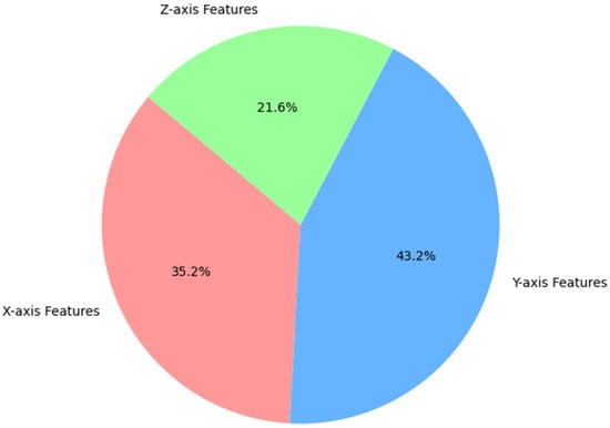
Figure A1.
The X-, Y-, and Z-axis feature ratio of the features selected by each FS method.
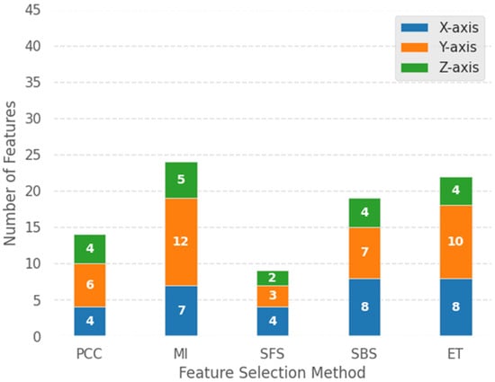
Figure A2.
Detailed number of X-, Y-, and Z-axis features selected by each FS method.
Observing Figure A1, the feature with the highest proportion selected by the five methods after summarization is the Y-axis feature, accounting for 43.2%. The next is the X-axis feature, accounting for 35.2%. Finally, the Z-axis feature only accounts for 21.6%. The analysis results show that the features of the X axis and Y axis are selected with a larger proportion.
Combined with the analysis of the original data in the previous Section 3.2 and observing Figure A1, we can draw the conclusion that the features selected by FS are in line with the analysis of the physical characteristics of the original data in Section 3.2. In general, compared with the vertical direction (Z axis), the acceleration data collected from the collision in the horizontal directions (X axis and Y axis) has greater volatility. The Y-axis features have more discriminative power for classification, so after using FS, the selected features reach the highest proportion.
Specifically, by observing Figure A2, and taking ET as an example—which was selected as part of the best combination (KNN and ET) in this study—ET selected 8 X-axis features and 10 Y-axis features, but only 4 Z-axis features. This result is consistent with the above-mentioned characteristic properties. Through the analysis and summary of Figure A1 and Figure A2, the FS method used in this study effectively selected the features of the original data, maintained the original physical properties of the data, and confirmed the feasibility of this study.
Appendix A.4. Performance of a Single Multi-Class Classification System
Table A12, Table A13 and Table A14 show the precision, recall, and F1 score of the model in the single multi-class classification system using various FS methods to select features. In general, the three indicators are close to the accuracy of each ML model, which means that each combination of ML model and FS method has real good performance. Using the top-performing combination of KNN and ET, which achieved an accuracy of 97.1% in this study, as an example, its precision, recall, and F1 score are 97.6%, 97.4%, and 97.4%, respectively. These three metrics slightly surpass the accuracy rate, suggesting that the stability of KNN and ET is sufficient to validate the credibility of the best model selected in this study.
Table A12.
Precision of different FS methods and ML models.
Table A12.
Precision of different FS methods and ML models.
| Model | Original | PCC | MI | SFS | SBS | ET |
|---|---|---|---|---|---|---|
| DT | 93.2 | 93.6 | 94.2 | 94.0 | 93.1 | 94.5 |
| KNN | 93.6 | 93.4 | 96.9 | 94.8 | 96.8 | 97.6 |
| SVM | 95.4 | 95.3 | 97.1 | 95.4 | 97.2 | 97.7 |
| RF | 98.1 | 96.8 | 98.1 | 96.5 | 97.8 | 98.3 |
| XGBoost | 98.6 | 96.7 | 98.4 | 96.5 | 98.6 | 98.7 |
Table A13.
Recall of different FS methods and ML models.
Table A13.
Recall of different FS methods and ML models.
| Model | Original | PCC | MI | SFS | SBS | ET |
|---|---|---|---|---|---|---|
| DT | 92.9 | 93.4 | 94.0 | 93.7 | 92.7 | 94.2 |
| KNN | 93.1 | 92.8 | 96.7 | 94.5 | 96.7 | 97.4 |
| SVM | 94.9 | 95.1 | 97.0 | 95.0 | 97.1 | 97.6 |
| RF | 98.1 | 96.5 | 98.1 | 96.3 | 97.7 | 98.2 |
| XGBoost | 98.5 | 96.5 | 98.4 | 96.3 | 98.5 | 98.7 |
Table A14.
F1 score of different FS methods and ML models.
Table A14.
F1 score of different FS methods and ML models.
| Model | Original | PCC | MI | SFS | SBS | ET |
|---|---|---|---|---|---|---|
| DT | 92.9 | 93.4 | 94.0 | 93.7 | 92.6 | 94.2 |
| KNN | 92.9 | 92.9 | 96.7 | 94.4 | 96.7 | 97.4 |
| SVM | 94.9 | 95.1 | 96.9 | 94.9 | 97.1 | 97.5 |
| RF | 98.0 | 96.4 | 98.0 | 96.3 | 97.7 | 98.2 |
| XGBoost | 98.5 | 96.4 | 98.3 | 96.3 | 98.5 | 98.6 |
Appendix B
Appendix B.1. Statistical Analysis of Execution Times for the Best Combination
Based on Table A2, for execution time, this study also performed two separate Friedman tests, using models execution time as the treatment group’s H0 and H1:
H0:
Under the original dataset features and the five FS methods, there is no significant difference in execution time among the five models (DT, KNN, SVM, RF, XGBoost).
H1:
There is a significant difference in execution time among the five models.
For the model-level Friedman test of execution time (grouped by model), the test statistic χ2 = 24.0 and p = 7.987 × 10⁻⁵. Because p < 0.05, we reject H0, indicating that there is a statistically significant difference in the execution time of the five models under the six FS methods. In other words, at least one model’s performance differs from the others by more than random error can explain. From the observed results, complex models (such as RF and XGBoost) consistently require longer execution times than simpler models (such as DT and KNN).
Using FS methods as the treatment group’s H0 and H1:
H0:
Under the five models, there is no significant difference in execution time between the original dataset features and the five FS methods (PCC, MI, SFS, SBS, ET).
H1:
There is a significant difference in execution time between the original dataset features and the five FS methods.
Next, for the FS method-level Friedman test for execution time (grouping by FS method), the test statistic χ2 = 22.471 and p = 0.0004259. Because p < 0.05, we reject H0, indicating that there is a statistically significant difference in the execution time between the original dataset features and the five FS methods under the five models. This demonstrates that FS methods can indeed optimize the model’s execution time by reducing features in the original dataset.
Appendix B.2. Statistical Analysis of CPU Utilization for the Best Combination
Based on Table A3, for CPU utilization, we also performed two separate Friedman tests, using models CPU utilization as the treatment group’s H0 and H1:
H0:
Under the original dataset features plus five FS methods, there is no significant difference in CPU utilization among the five models (DT, KNN, SVM, RF, XGBoost).
H1:
There is a significant difference in CPU utilization among the five models.
For CPU utilization, the model-level Friedman test results show a test statistic of 16.84 and a p-value of 0.002076 (rounded). Because p < 0.05, we reject the null hypothesis, indicating that there is a statistically significant difference in the CPU utilization of the five models under the six FS methods. Specifically, complex models (such as XGBoost and RF) have significantly higher CPU utilization than simpler models (such as DT and KNN), with XGBoost showing the highest resource consumption under all conditions, indicating a positive correlation between model complexity and CPU consumption.
Using FS methods as the treatment group’s H0 and H1:
H0:
Under the five models, there is no significant difference in the CPU utilization between the original dataset features and the five FS methods (PCC, MI, SFS, SBS, ET).
H1:
There is a significant difference in CPU utilization between the original dataset features and the five FS methods.
For CPU utilization, the FS method-level Friedman test results show a test statistic of 13.918 and a p-value of 0.016138 (rounded). Because of p < 0.05, we reject the null hypothesis, indicating that there is a statistically significant difference in CPU utilization between the original dataset features and the five FS methods under the five models. Further examination reveals that FS methods (such as PCC and ET) have significantly lower CPU utilization than the original dataset features, suggesting that FS can effectively reduce resource consumption in the model.
References
- Kaup, M.; Łozowicka, D.; Baszak, K.; Ślączka, W.; Kalbarczyk-Jedynak, A. Review of the Container Ship Loading Model—Cause Analysis of Cargo Damage and/or Loss. Pol. Marit. Res. 2022, 29, 26–35. [Google Scholar] [CrossRef]
- International Forwarding Association. Cargo Damage, Types and Impact—International Forwarding Association Blog; International Forwarding Association: Lisbon, Portugal, 2023; Available online: https://ifa-forwarding.net/blog/uncategorized/cargo-damage-types-and-impact/ (accessed on 17 November 2023).
- Tseng, W.-J.; Ding, J.-F.; Chen, Y.-C. Evaluating Key Risk Factors Affecting Cargo Damages on Export Operations for Container Carriers in Taiwan. Int. J. Marit. Eng. 2018, 160, 1076. [Google Scholar] [CrossRef]
- Navigating Stormy Waters. Review of Maritime Transport/United Nations Conference on Trade and Development, Geneva; United Nations: Geneva, Switzerland, 2022; ISBN 978-92-1-113073-7. [Google Scholar]
- Pamucar, D.; Faruk Görçün, Ö. Evaluation of the European Container Ports Using a New Hybrid Fuzzy LBWA-CoCoSo’B Techniques. Expert Syst. Appl. 2022, 203, 117463. [Google Scholar] [CrossRef]
- Tsolakis, N.; Zissis, D.; Papaefthimiou, S.; Korfiatis, N. Towards AI Driven Environmental Sustainability: An Application of Automated Logistics in Container Port Terminals. Int. J. Prod. Res. 2022, 60, 4508–4528. [Google Scholar] [CrossRef]
- Chen, R.; Meng, Q.; Jia, P. Container Port Drayage Operations and Management: Past and Future. Transp. Res. Part E Logist. Transp. Rev. 2022, 159, 102633. [Google Scholar] [CrossRef]
- Nguyen, P.N.; Woo, S.-H.; Beresford, A.; Pettit, S. Competition, Market Concentration, and Relative Efficiency of Major Container Ports in Southeast Asia. J. Transp. Geogr. 2020, 83, 102653. [Google Scholar] [CrossRef]
- Gunes, B.; Kayisoglu, G.; Bolat, P. Cyber Security Risk Assessment for Seaports: A Case Study of a Container Port. Comput. Secur. 2021, 103, 102196. [Google Scholar] [CrossRef]
- Russell, D.; Ruamsook, K.; Roso, V. Managing Supply Chain Uncertainty by Building Flexibility in Container Port Capacity: A Logistics Triad Perspective and the COVID-19 Case. Marit. Econ. Logist. 2022, 24, 92–113. [Google Scholar]
- Baştuğ, S.; Şakar, G.D.; Gülmez, S. An Application of Brand Personality Dimensions to Container Ports: A Place Branding Perspective. J. Transp. Geogr. 2020, 82, 102552. [Google Scholar] [CrossRef]
- Bee, G.R.; Hontz, L.R. Detection and Prevention of Post-Processing Container Handling Damage. J. Food Prot. 1980, 43, 458–461. [Google Scholar] [CrossRef]
- Callesen, F.G.; Blinkenberg-Thrane, M.; Taylor, J.R.; Kozine, I. Container Ships: Fire-Related Risks. J. Mar. Eng. Technol. 2021, 20, 262–277. [Google Scholar] [CrossRef]
- Eglynas, T.; Jakovlev, S.; Bogdevicius, M.; Didžiokas, R.; Andziulis, A.; Lenkauskas, T. Concept of Cargo Security Assurance in an Intermodal Transportation. In Marine Navigation and Safety of Sea Transportation: Maritime Transport and Shipping; CRC Press: Boca Raton, FL, USA, 2013; pp. 223–226. [Google Scholar] [CrossRef]
- Delgado, G.; Cortés, A.; García, S.; Loyo, E.; Berasategi, M.; Aranjuelo, N. Methodology for Generating Synthetic Labeled Datasets for Visual Container Inspection. Transp. Res. Part E Logist. Transp. Rev. 2023, 175, 103174. [Google Scholar] [CrossRef]
- International Maritime Organization. Casualty-Related Matters: Reports on Marine Casualties and Incidents. In MSC-MEPC.3/Circ.3; International Maritime Organization: London, UK, 2008; pp. 1–7. Available online: https://wwwcdn.imo.org/localresources/en/OurWork/MSAS/Documents/MSC-MEPC.3-Circ.3.pdf (accessed on 25 May 2025).
- Delgado, G.; Cortés, A.; Loyo, E. Pipeline for Visual Container Inspection Application Using Deep Learning. In Proceedings of the 14th International Joint Conference on Computational Intelligence, Valletta, Malta, 24–26 October 2022; SCITEPRESS—Science and Technology Publications: Setúbal, Portugal, 2022; pp. 404–411. [Google Scholar]
- Bahrami, Z.; Zhang, R.; Wang, T.; Liu, Z. An End-to-End Framework for Shipping Container Corrosion Defect Inspection. IEEE Trans. Instrum. Meas. 2022, 71, 5020814. [Google Scholar] [CrossRef]
- Wang, Z.; Gao, J.; Zeng, Q.; Sun, Y. Multitype Damage Detection of Container Using CNN Based on Transfer Learning. Math. Probl. Eng. 2021, 2021, e5395494. [Google Scholar] [CrossRef]
- Vaz, A.; Ramachandran, L. Cargo Damage and Prevention Measures to Reduce Product Damage in Malaysia. 2023. Available online: https://dnd.com.my/dwnlds/news/Cargo_damage_and_prevention_measures_in_Malaysia.pdf (accessed on 28 February 2025).
- Dzemydienė, D.; Burinskienė, A.; Čižiūnienė, K.; Miliauskas, A. Development of E-Service Provision System Architecture Based on IoT and WSNs for Monitoring and Management of Freight Intermodal Transportation. Sensors 2023, 23, 2831. [Google Scholar] [CrossRef]
- Bauk, S.; Radulović, A.; Dzankic, R. Physical Computing in a Freight Container Tracking: An Experiment. In Proceedings of the 2023 12th Mediterranean Conference on Embedded Computing (MECO), Budva, Montenegro, 6–10 June 2023; pp. 1–4. [Google Scholar]
- Li, Q.; Cao, X.; Xu, H. In-Transit Status Perception of Freight Containers Logistics Based on Multi-Sensor Information; Springer: Berlin/Heidelberg, Germany, 2016; Volume 9864, pp. 503–512. [Google Scholar]
- Song, Y.; Van Hoecke, E.; Madhu, N. Portable and Non-Intrusive Fill-State Detection for Liquid-Freight Containers Based on Vibration Signals. Sensors 2022, 22, 7901. [Google Scholar] [CrossRef]
- Lee, J.; Lee, J.-Y.; Cho, S.-M.; Yoon, K.-C.; Kim, Y.J.; Kim, K.G. Design of Automatic Hand Sanitizer System Compatible with Various Containers. Healthc. Inf. Res. 2020, 26, 243–247. [Google Scholar] [CrossRef]
- Jakovlev, S.; Eglynas, T.; Voznak, M.; Jusis, M.; Partila, P.; Tovarek, J.; Jankunas, V. Detecting Shipping Container Impacts with Vertical Cell Guides inside Container Ships during Handling Operations. Sensors 2022, 22, 2752. [Google Scholar] [CrossRef]
- Liu, D.; Shi, G. Ship Collision Risk Assessment Based on Collision Detection Algorithm. IEEE Access 2020, 8, 161969–161980. [Google Scholar] [CrossRef]
- Shi, J.; Liu, Z. Track Pairs Collision Detection with Applications to Ship Collision Risk Assessment. J. Mar. Sci. Eng. 2022, 10, 216. [Google Scholar] [CrossRef]
- Najafi Mohsenabad, H.; Tut, M.A. Optimizing Cybersecurity Attack Detection in Computer Networks: A Comparative Analysis of Bio-Inspired Optimization Algorithms Using the CSE-CIC-IDS 2018 Dataset. Appl. Sci. 2024, 14, 1044. [Google Scholar] [CrossRef]
- Ahmed, N.; Rafiq, J.I.; Islam, M.R. Enhanced Human Activity Recognition Based on Smartphone Sensor Data Using Hybrid Feature Selection Model. Sensors 2020, 20, 317. [Google Scholar] [CrossRef] [PubMed]
- Shaban, W.M.; Rabie, A.H.; Saleh, A.I.; Abo-Elsoud, M.A. A New COVID-19 Patients Detection Strategy (CPDS) Based on Hybrid Feature Selection and Enhanced KNN Classifier. Knowl. Based Syst. 2020, 205, 106270. [Google Scholar] [CrossRef]
- Sun, Y.; Cao, Y.; Li, P.; Su, S. Fault Diagnosis for RPMs Based on Novel Weighted Multi-Scale Fractional Permutation Entropy Improved by Multi-Scale Algorithm and PSO. IEEE Trans. Veh. Technol. 2024, 73, 11072–11081. [Google Scholar] [CrossRef]
- Khan, J.; Alam, A.; Lee, Y. Intelligent Hybrid Feature Selection for Textual Sentiment Classification. IEEE Access 2021, 9, 140590–140608. [Google Scholar] [CrossRef]
- Buckley, T.; Ghosh, B.; Pakrashi, V. A Feature Extraction & Selection Benchmark for Structural Health Monitoring. Struct. Health Monit. 2022, 22, 2082–2127. [Google Scholar] [CrossRef]
- Jiang, S.; Zhao, J.; Xu, X. SLGBM: An Intrusion Detection Mechanism for Wireless Sensor Networks in Smart Environments. IEEE J. Mag. 2020, 8, 169548–169558. [Google Scholar]
- Zhou, M.; Cui, M.; Xu, D.; Zhu, S.; Zhao, Z.; Abusorrah, A. Evolutionary Optimization Methods for High-Dimensional Expensive Problems: A Survey. IEEE/CAA J. Autom. Sin. 2024, 11, 1092–1105. [Google Scholar] [CrossRef]
- Zhou, J.; Wu, Q.; Zhou, M.; Wen, J.; Al-Turki, Y.; Abusorrah, A. LAGAM: A Length-Adaptive Genetic Algorithm with Markov Blanket for High-Dimensional Feature Selection in Classification. IEEE Trans. Cybern. 2023, 53, 6858–6869. [Google Scholar] [CrossRef]
- Tarkhaneh, O.; Nguyen, T.T.; Mazaheri, S. A Novel Wrapper-Based Feature Subset Selection Method Using Modified Binary Differential Evolution Algorithm. Inf. Sci. 2021, 565, 278–305. [Google Scholar] [CrossRef]
- Jiao, R.; Nguyen, B.H.; Xue, B.; Zhang, M. A Survey on Evolutionary Multiobjective Feature Selection in Classification: Approaches, Applications, and Challenges. IEEE Trans. Evol. Comput. 2024, 28, 1156–1176. [Google Scholar] [CrossRef]
- Islam, M.R.; Lima, A.A.; Das, S.C.; Mridha, M.F.; Prodeep, A.R.; Watanobe, Y. A Comprehensive Survey on the Process, Methods, Evaluation, and Challenges of Feature Selection. IEEE Access 2022, 10, 99595–99632. [Google Scholar] [CrossRef]
- Geurts, P.; Ernst, D.; Wehenkel, L. Extremely Randomized Trees. Mach. Learn. 2006, 63, 3–42. [Google Scholar] [CrossRef]
- Quinlan, J.R. Induction of Decision Trees. Mach. Learn. 1986, 1, 81–106. [Google Scholar] [CrossRef]
- Cover, T.; Hart, P. Nearest Neighbor Pattern Classification. IEEE Trans. Inf. Theory 1967, 13, 21–27. [Google Scholar] [CrossRef]
- Cortes, C.; Vapnik, V. Support-Vector Networks. Mach. Learn. 1995, 20, 273–297. [Google Scholar] [CrossRef]
- Breiman, L. Random Forests. Mach. Learn. 2001, 45, 5–32. [Google Scholar] [CrossRef]
- Chen, T.; Guestrin, C. XGBoost: A Scalable Tree Boosting System. In Proceedings of the 22nd ACM SIGKDD International Conference on Knowledge Discovery and Data Mining, San Francisco, CA, USA, 13–17 August 2016; pp. 785–794. [Google Scholar] [CrossRef]
- Naiem, S.; Khedr, A.E.; Idrees, A.; Marie, M. Enhancing the Efficiency of Gaussian Naïve Bayes Machine Learning Classifier in the Detection of DDOS in Cloud Computing. IEEE Access 2023, 11, 124597–124608. [Google Scholar] [CrossRef]
- Greenacre, M.; Groenen, P.J.F.; Hastie, T.; D’enza, A.I.; Markos, A.; Tuzhilina, E. Principal Component Analysis. Nat. Rev. Methods Primers 2022, 2, 100. [Google Scholar] [CrossRef]
- Zimmerman, D.W.; Zumbo, B.D. Relative Power of the Wilcoxon Test, the Friedman Test, and Repeated-Measures ANOVA on Ranks. J. Exp. Educ. 1993, 62, 75–86. [Google Scholar] [CrossRef]
Disclaimer/Publisher’s Note: The statements, opinions and data contained in all publications are solely those of the individual author(s) and contributor(s) and not of MDPI and/or the editor(s). MDPI and/or the editor(s) disclaim responsibility for any injury to people or property resulting from any ideas, methods, instructions or products referred to in the content. |
© 2025 by the authors. Licensee MDPI, Basel, Switzerland. This article is an open access article distributed under the terms and conditions of the Creative Commons Attribution (CC BY) license (https://creativecommons.org/licenses/by/4.0/).