An Investigation of Reverberation Received by a Vertical Antenna at Short Ranges in Shallow Seas

Abstract

In this paper, we discuss the results of hydroacoustic sounding in the frequency range of units of kHz, conducted during voyage No. 90 of the research vessel “Akademik Mstislav Keldysh”. The employment of a vertical antenna array and electronic phasing to the recorded data made it possible to determine both the reflection coefficient from the bottom at incidence close to normal, and the diffuse scattering coefficients at oblique angles for the surface and the bottom. Based on the processing of experimental data, and with the help of computer modeling, an analysis of the structure of hydroacoustic signals scattered by the bottom and free surface of water was carried out. An approach combining the Green’s function and the scattering function was used to model the reverberation signal. The models of formation of the Doppler spectrum of the scattered acoustic signal were refined, taking into account the influence of sound propagation conditions in the marine environment. The comparison of the results of experimental studies of bottom reverberation in the waters of the Barents and Kara Seas with numerical calculations of the ray structure of the acoustic field demonstrates good agreement.

1. Introduction

The marine environment is a multifaceted system that directly affects human life. Its study is carried out in various directions and methods; for example, consider the study of the top relief, processes flowing in the water column and on its surface, the development of new marine technology, and the study of hydrobionts [1,2,3]. One of the most important tasks associated with this topic is the study of the propagation of sound signals in the water column. The marine environment is a complex channel for the propagation of acoustic signals [4]. Multipath phenomena and reverberation lead to the distortion and delay of transmitted signals, which significantly complicates such operations as, for example, bottom survey, search for sunken objects, as well as navigation and communication with underwater vehicles. The influence of multipath and reverberation is especially evident in the shelf zone, at shallow depths [5,6]. For example, the Arctic seas, which include the Barents and Kara Seas, are characterized by a very wide shelf. In recent decades, interest in the Arctic region has increased significantly due to its role in the global climate system, as well as its important economic and environmental significance [7]. Scientific research in the Arctic is carried out, among other things, using hydroacoustic systems [8,9], for which it is important to take into account the influence of multipath and reverberation.

Calculations of sound propagation taking into account multiple reflections from the surface and bottom, as well as refraction in the water column, can be performed analytically for a number of reference waveguides [10], and for real conditions or more complex parameters of model problems, they are performed by numerical methods [11,12]. Unfortunately, there is no similarly established approach for modeling reverberation. Research is conducted in two directions: first, refining specific sound-scattering coefficients on a rough surface [13] or an uneven bottom [14]; second, incorporating these coefficients into a general propagation model for modeling received signals under specific experimental conditions [15,16]. For this purpose, mode [17] and ray [18,19,20] approaches can be used. Probably, the highest accuracy of modeling can be achieved using the finite element method [21], but it has the highest computational costs. For many applications, the energy approach of multiplying the scattering force by the illuminated area, or, in the case of volume scattering, by the pulse volume [4,22], appears to be sufficient.

Specific characteristics of the environment required for the operation of the above models exhibit significant regional dependence. Although there are global databases of sound-velocity profiles with seasonal dependence and a worldwide map of the bottom relief, these data are often insufficient for reliable calculations for a specific water area. The construction of more detailed, regional models of sound propagation is an important task [23]. For example, with respect to the Kara Sea shelf discussed below, a number of authors claim the presence of areas of a bottom with significantly heterogeneous characteristics [24]. Actual values of bottom scattering strength are of interest too [25].

Numerous experimental studies on surface and bottom scattering strength have been conducted using explosive sources [22]. Subsequent research employed coherent pings and chirped signals [16,19,20]. Notably, the first mentioned study [16] was carried out in a shallow water environment, whereas the second one [19,20] took place at greater depths ranging from 500 to 1000 m. The use of continuously repeated chirped signals, also known as pulse-train frequency modulated (PTFM) or continuous active sonar (CAS), enables the measurement of the Doppler spread of the reverberation signal. In study [26], it was found that the scattered signal’s Doppler shift primarily resulted from the fact that the experiment was arranged with a towed array. In this project, we investigated bottom and surface reflection and scattering using pings and chirps in a shallow water area. Additionally, we analyzed the Doppler spread of surface-scattered signals using PTFM signals at stationary ship positions.

In this paper, we consider the results of a full-scale experiment carried out during voyage No. 90 of the research vessel “Akademik Mstislav Keldysh” (RV “AMK”) in the Barents and Kara Seas (along the Northern Sea Route). While the vessel was drifting, acoustic signals were sounded at stations in the frequency range of units of kHz. The data obtained by the vertical antenna array made it possible to determine both the reflection coefficient from the bottom at incidence close to normal and the diffuse scattering coefficients at oblique angles for the surface and bottom. The analysis of the experimental results is complemented by computer simulation. By generalizing the ray model of sound propagation [27], a method for the numerical modeling of reverberation in the shallow shelf zone of the northern seas was developed. The reflection of sound from a rough surface is, in our opinion, the most complex case of reverberation, since it is accompanied by a Doppler frequency shift, for the correct description of which a separate model is used [28].

The article is structured as follows. The Section 1 describes the experimental material of the hydroacoustic sounding of shallow water, the types of emitted signals, and the parameters of the medium. The Section 2 describes the proposed approach for calculating ray trajectories in the model of reverberation received by a vertical antenna at short distances in shallow water. The Section 3 contains the results of processing experimental data and computer simulation. The conclusion summarizes the results of the article.

2. Materials and Methods

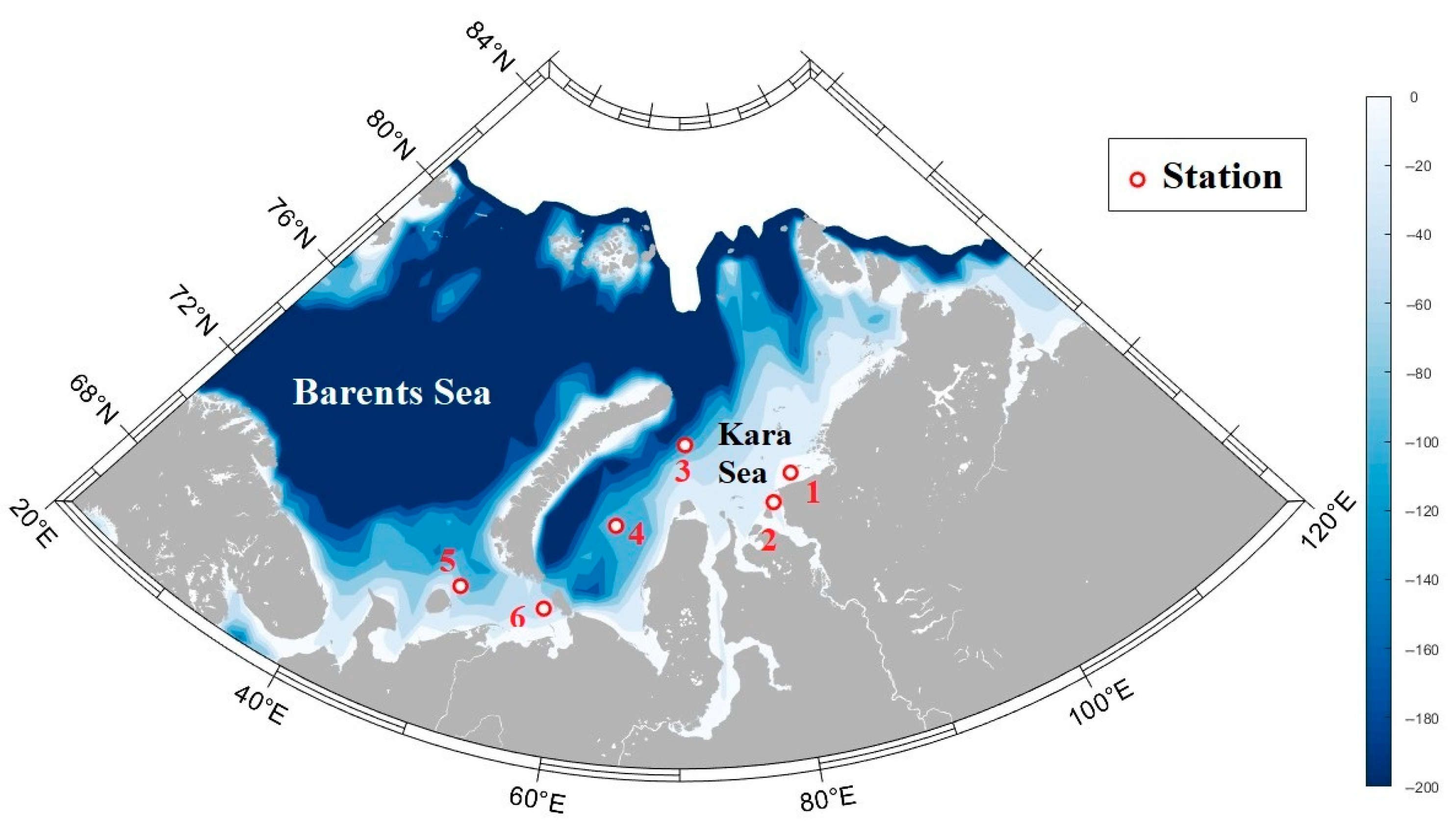
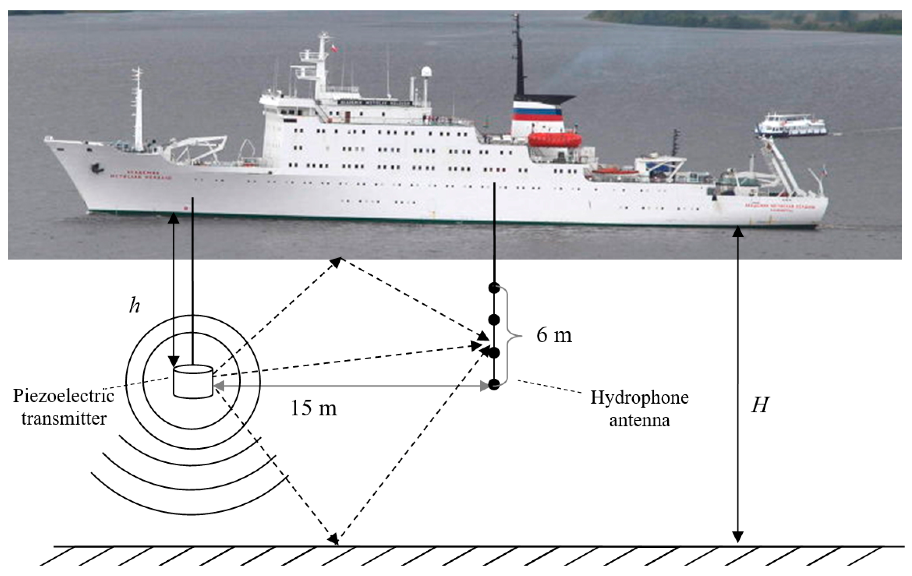
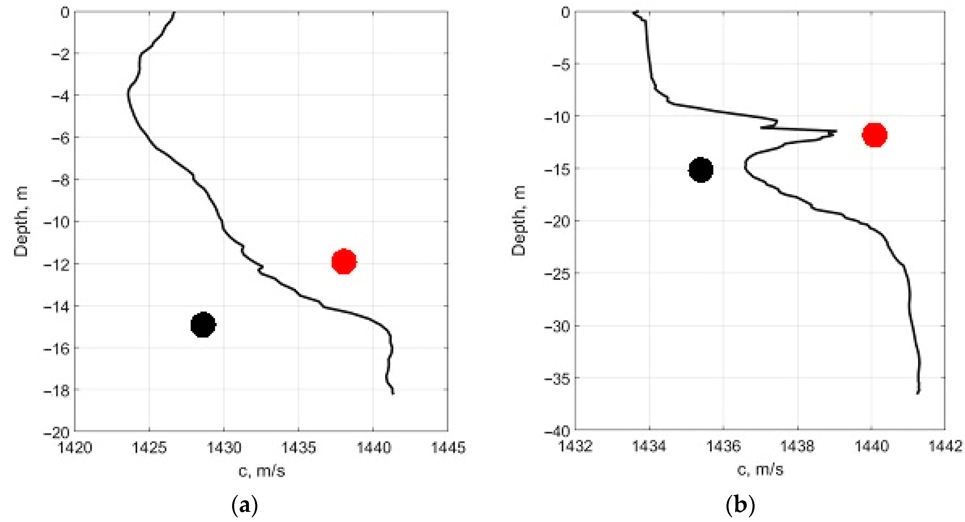
2.1. Experimental Information

In October–November 2022, during cruise No. 90 of the research vessel “AMK”, a full-scale experiment was conducted, aimed at studying sound scattering in the waters of the Barents and Kara Seas. The map of the work area is shown in Figure 1; hydroacoustic measurements were carried out at 6 stations while the vessel was drifting.

The equipment was located at a level $h$ from the water surface equal to 15 or 30 m, depending on the depth of the place, as shown in the experimental scheme in Figure 2. The work was carried out in the shelf zone with depths in the range from 19 to 70 m. The emitting and receiving systems in the experiments were spaced from each other by 15 m, with the center of the receiving antenna located 3 m above the emitter. The probing signals were generated by an omnidirectional piezoceramic emitter, and the scattered signal was recorded by a 32-element hydrophone antenna located vertically. The distance between the receiving elements of the antenna was 20 cm, which allowed us to operate with a filled aperture up to a frequency of ~3.7 kHz. Each sensor had a smooth response in the operating frequency range of 5–12,000 Hz and a sensitivity of about 5 mV/Pa. The sensitivity difference in all sensors was less than 3 dB.

Piezoceramic-type hydrophones were equipped with preamplifiers and connected by a common multi-core cable. The signals were sent via this cable to a common 32-channel analog-to-digital converter (ADC) located in a sealed small container at the end of the antenna underwater. The ADC with its accompanying electronic unit transmitted data via Ethernet cable to the surface. This scheme allowed us to reduce the influence of electrical interference, but the range of stable information transmission via an Ethernet cable was 50 m. In this experiment, increasing the distance was not required, but, if necessary, signal repeaters should be installed in a cable line operating according to this standard.

The probing signals were generated by the digital-to-analog converter of the external sound card and amplified by the concert amplifier “Cerwin-Vega CXA-10” (Cerwin-Vega Inc., Los Angeles, CA, USA) with a nominal power of 3 kW. To match the output of the class AB amplifier with the capacitive load, a high-current inductor coil was used, i.e., this circuit design formed a series resonant circuit: emitter–inductor coil–amplifier. The amplitude of the emitted signals at 1 m was of the order of 1 kPa at a frequency of 2 kHz., i.e., the source level was 180 dB relative to 1 μPa, which falls below the threshold for pulsed signals within this frequency range, above which such signals may become hazardous to marine mammals [29].

In the process of researching the bottom reverberation, we carried out probing with sequential emission of tonal pulses at frequencies of 1000, 1500, 2000… 3500 Hz with a duration of 3 ms with a period of 0.5 s between adjacent pulses; the total period of the pulse sequence is 2.5 s. The Fourier transform of this signal with a short and long window is shown in Figure 3a,b. To research surface reverberation, a signal with continuous frequency sweeping was used in the form of a packet of pulses with linear frequency modulation (chirp) at a frequency of 1500–2500 Hz, where each individual chirp took 0.2 s (this signal was also used to analyze bottom reverberation). The Fourier transform with a short window results in a saw-shaped spectrogram (Figure 3c). The long-window Fourier transform shows that the signal has a ridged spectrum (Figure 3e), which is a consequence of the strict periodicity of the signal and allows for an accurate determination of the Doppler frequency while maintaining the overall signal bandwidth; Figure 3d shows the signal spectrum in an extended frequency range.

The received signal is multiplied by an identical “saw”, but with a frequency shift, which is similar to the use of a tracking heterodyne. Taking into account the propagation time in the medium, the carrier frequency of the reflected signal lags behind the current heterodyne frequency and, according to this principle, the range is identified with the value of the difference frequency. Next, the algorithm monitors the phase of the signal at a certain difference frequency, this phase smoothly changes from pulse to pulse within the packet, due to which it is possible to determine the Doppler frequency for this signal [30]. Readers might also be interested to know the other way to process chirps with a Fractional Fourier transform [31].

Some insights into how the design of our experimental setup facilitated the investigation of surface scattering phenomena follow. Surface scattering at high frequencies is predominantly influenced by bubbles even under minimal wind conditions [4]. Within the kilohertz range, sound reflections remain contingent upon the contour of the air–water boundary, and the wavelength is short enough to allow for the distinct separation of various reflections such as direct impingement, primary, secondary, and subsequent bounces off the water’s surface. Furthermore, employing a continuous transmission technique with a 15 m separation between transmitter and receiver ensured that the received signals were free from distortion caused by signal clipping effects.

Next, let us closely consider the results obtained for two measurement areas: stations 1 and 2. Both stations were located in the Kara Sea with depths of 19.7 and 37.2 m with a relatively flat bottom topography. During operation at the stations, different hydrometeorological conditions were observed: station 1 was characterized by weak waves (the length of the energy-carrying wind wave is 12 m, the significant height is 0.3 m); station 2 was characterized by strong waves (the length of the energy-carrying wind wave is 80 m, the significant height is 1.2 m). When carrying out the calculation of acoustic rays (the model of which is given in the next section), sound speed profiles obtained experimentally for each station were used; examples of such profiles for stations 1 and 2 are shown in Figure 4a,b. The black dots on the graphs show the location of the sound source, the red ones the position of the center of the receiving antenna.

2.2. Model

To develop an acoustic model for the formation of Doppler scattering spectra using the ray approximation, a model of signal reflection from the free surface of the water and from the bottom emitted by a point source located in the water column is constructed. The constructed model takes into account the influence of the sound-velocity profile on the propagation of acoustic rays. For this purpose, the method of stepwise approximation of the depth dependence of the sound-velocity profile is used: the water column is divided by depth into horizontally homogeneous layers, where the sound velocity is considered constant and changes abruptly at the boundaries of these layers (Figure 5a). Within the ray approximation, it is considered that a fan of rays is emitted from the source with a given angular step with the initial (zero) exit angle $\phi$ counted from the vertical (Figure 5b). Each water layer is characterized by thickness $h_i$, sound velocity ${\mathrm{c}}_i$ and density ${\rho }_i$. The source and receiver are located at depths $z_S$ and ${\mathrm{z}}_R$, respectively. To calculate the scattering spectra, we consider rays emerging from the source upwards to the free surface of the water at an exit angle of ${\phi }_j$ to the vertical, and rays emerging towards the bottom at an angle of ${\phi }_k$ to the vertical, both of which are taken into account. For all rays, the coordinates of the passage of the layer boundaries ($x^j$, $x^k$), arrival times, distances, and signal amplitudes at the boundaries are calculated.

Each ray undergoes refraction at the boundaries of water layers. The coefficients of reflection and refraction are calculated using Snell’s law [10], which also takes into account the critical angles of incidence at the interface at which total internal reflection occurs and the acoustic beam does not reach the surface of the water or the boundary of the water column with the bottom. For a local water–water boundary, the reflection coefficient of each ray incident at an angle ${\alpha }_i$ on the boundary of the $i$ and $\left(i+1\right)$ water layer ($i=1÷N_w, { N}_w$ is the number of layers into which the water column is divided) is expressed as:

$$V_i={\displaystyle \frac{m_i·cos{\alpha }_i-\sqrt{n_i^2-{sin}^2{\alpha }_i}}{m_i·cos{\alpha }_i+\sqrt{n_i^2-{sin}^2{\alpha }_i}}},$$

(1)

the transmission coefficient at this boundary is expressed as:

$$W_i={\displaystyle \frac{2·m_i·cos{\alpha }_i}{m_i·cos{\alpha }_i+\sqrt{n_i^2-{sin}^2{\alpha }_i}}},$$

(2)

where $m_i={\rho }_{i+1}/{\rho }_i$, $n_i=c_i^w/c_{i+1}^w$, ${\rho }_i$ is the density of water in the $i$-th layer, $c_i$ is the speed of sound in the $i$-th layer, and $\mathrm{s}\mathrm{i}\mathrm{n}\left({\alpha }_i\right)=n_i·sin\left({\alpha }_{i+1}\right)$ is the refraction angle. These expressions are also valid for the water–air boundary.

The reflection coefficient at the water–bottom boundary is calculated as:

$$V={\displaystyle \frac{Z_{i+1}^P·{cos}^2\left(2{\vartheta }_{i+1}^{SV}\right)+Z_{i+1}^{SV}·{sin}^2\left(2{\vartheta }_{i+1}^{SV}\right)-Z_i}{Z_{i+1}^P·{cos}^2\left(2{\vartheta }_{i+1}^{SV}\right)+Z_{i+1}^{SV}·{sin}^2\left(2{\vartheta }_{i+1}^{SV}\right)+Z_i}},$$

(3)

where $sin{\vartheta }_{i+1}^P=sin{\alpha }_i{\displaystyle \frac{{\mathrm{c}}_{i+1}^P}{{\mathrm{c}}_i^w}}$, $sin{\vartheta }_{i+1}^{SV}=sin{\alpha }_i{\displaystyle \frac{{\mathrm{c}}_{i+1}^{SV}}{{\mathrm{c}}_i^w}}$, $Z_i={\displaystyle \frac{{\rho }_i{\mathrm{c}}_i^w}{cos{\alpha }_i}}$, $Z_{i+1}^P={\displaystyle \frac{{\rho }_{i+1}{\mathrm{c}}_{i+1}^P}{cos{\vartheta }_{i+1}^P}}$, $Z_{i+1}^{SV}={\displaystyle \frac{{\rho }_{i+1}{\mathrm{c}}_{i+1}^{SV}}{cos{\vartheta }_{i+1}^{SV}}}$, $Z$ is the impedance of the corresponding layer, $c^P$, $c^{SV}$ are the velocities of longitudinal and transverse waves in the bottom, equal to 2200 m/s and 1200 m/s, respectively. The density of the bottom layer ${\rho }_{i+1}$ for calculations is taken to be 1190 kg/m³. These values are typical for sandy bottom.

The developed calculation model includes the following groups of rays (Figure 6): 1—rays going from the source to the water surface; 2—rays going along the trajectory source–bottom–water surface; 3—source–water surface–bottom–water surface; 4—source–bottom–water surface–bottom–water surface; 5—source–bottom; 6—source–bottom–water surface–bottom, 7—from the source to the bottom. Rays from some groups in most cases are continued in the form of rays from other groups. Taking into account all the specified groups of rays, once and repeatedly reflected from the bottom and the water surface, helps to clarify the numerical calculations for a better description of the experimental data. To compare the model data with the experimental data, estimates of the arrival times of all the above groups of rays were obtained depending on the vertical exit angle $\phi$. The results of the comparison are given in the next section.

An approach combining Green’s function and the scattering function is employed to simulate a reverberation signal [32]. Certain simplifications are introduced to derive computational formulas in a more concise format. Consider a sphere of a unit radius $r_0=1m$ and the source creates uniform amplitude p₀ on it. Next, we consider a ray tube between rays emerging from the source at angles ${\phi }_j$ and ${\phi }_{j+1}$ to the vertical. So, this ray tube carries power proportional to a spherical layer between ${\phi }_j$ and ${\phi }_{j+1}$ vertical angles that is:

$$s_0=2\pi sin\phi ∆\phi .$$

(4)

Let both beams be emitted into the upper half-plane from the source and reach the surface at points with coordinates $x^{\left(j\right)}$ and $x^{(j+1)}$, respectively. The angles of incidence to the vertical are ${\alpha }^{\left(j\right)}$ and ${\alpha }^{(j+1)}$. The average intensity of the incident field in this area can be determined based on the fact that the power, defined by (4), is distributed over the area that is cut off by the beams on the surface (taking into account the incidence at an angle). As a result, we have arrive at the expression:

$$p_{inc}^2={\displaystyle \frac{p_0^2{s}_0{r}_0^2}{s_{ray}cos\alpha }},$$

(5)

where

$$s_{ray}^{\left(j\right)}=\pi x^{\left(j\right)}\left(x^{(j+1)}-x^{(j-1)}\right).$$

(6)

The water–air boundary for ray calculations is considered flat. Surface disturbance is introduced into the ray model as follows. The entire illuminated area is considered a secondary source; each area $s^{\prime }$ creates a square of the pressure amplitude:

$$p_{scat}^2=p_{inc}^2\sigma \left(\alpha ,\beta \right)s^{\prime }{r}_0^{-2},$$

(7)

at a distance of $r_0=1m$ from itself. Here, $\alpha$ is, as above, the angle of incidence; $\beta$ is the scattering angle, also measured from the vertical, the coefficient $\sigma \left(\alpha ,\beta \right)$ is related to the scattering force (SF), introduced [22], by the equation: $SF=10\mathrm{l}\mathrm{g}\sigma \left(\alpha ,\beta \right)$. For initial estimates, we use the surface scattering force, given by the Marsh formula [22], generalized to the bistatic case:

$$\sigma \left(\alpha ,\beta \right)={10}^{-3.6}{\mathrm{c}\mathrm{t}\mathrm{g}}^2{\alpha }_j{·\mathrm{c}\mathrm{t}\mathrm{g}}^2{\beta }_j.$$

(8)

In the last chapter of this article, this value will be specified based on the analysis of the results of numerical modeling and experimental data. And, in turn, the illuminated area $s^{\prime }$ is determined by the minimum of two values:

$$s^{\prime }=min\left\{s_{ray}^{\left(j\right)},{\displaystyle \frac{cT{x}^{\left(j\right)}}{2sin{\alpha }^{\left(j\right)}}}2\pi \right\},$$

(9)

where $T$ is the pulse duration.

In general, to find the intensity of the scattered signal reaching the receiver, we would need to repeat the ray tracing procedure from each point $x^{\left(j\right)}$ and find those rays that return to the starting point. However, if we neglect the distance between the source and the receiver, which is acceptable in this case, we can optimize the procedure and use the return path of the same ray. Based on the reciprocity principle, the attenuation of the secondary source field $p_{scat}^2$ on the way to the starting point will be the same value determined by (5). As a result, we estimate that the signal, characterized by the square of the amplitude:

$$p_{rev}^2=p_0^2{\left({\displaystyle \frac{s_0{r}_0}{s_{ray}cos\alpha }}\right)}^2{s}^{\prime } \sigma \left(\alpha ,\alpha \right),$$

(10)

will be received by the antenna at angle ${\phi }^{\left(j\right)}$ with a delay of ${2t}^{\left(j\right)}$, where $t^{\left(j\right)}$ is the travel time to the surface.

Similarly to (10), the illumination of the surface by rays coming through the bottom is modeled, taking into account the absorption at each reflection from the bottom. There are also combinations characterized by different angles of incidence and scattering of sound; for example, the illumination of the surface by rays from group 1 and the return to the source by rays from group 2.

Formula (10) does not describe cases of specular reflection from the interfaces of media (the classical model is sufficient for this). Instead, (10) describes reverberation in the narrow sense, that is: diffuse reflection from the surface or bottom, which in experimental recordings stretches in the form of a trail (aftersound), following the arrival of specular reflection.

The calculation scheme is also generalized to bottom scattering; however, in this case $\sigma \left(\alpha ,\beta \right)$ obeys other laws [32,33] and depends significantly on the regional features of the bottom relief. In this work, for bottom scattering, we use the value specified by Formula (8) with a correction amplitude factor, which is selected based on experimental data for each station individually. Introducing such a coefficient allows us to compensate for the lack of information on the bottom parameters in the selected area, since in experimental simulation the bottom parameters are either known within a localized area or approximated based on general assumptions.

3. Results

3.1. General Results

The use of a linear receiving antenna made it possible to perform a phasing procedure for the recorded data to form spatial channels, dividing the received signal into sectors of width $∆\theta$, for a probing signal with a frequency of $f=2 \mathrm{k}\mathrm{H}\mathrm{z}$ $∆\theta =10°$. For example, with in-phase summation of the signal, a radiation pattern with an axis parallel to the surface was formed. In this geometry, a single pulse volume has the shape of a torus, i.e., there is no azimuth resolution. Further processing is performed as follows. In the signal band (tone pulse), we carry out frequency filtering and envelope calculationwith an averaging time equal to half the pulse duration. The results are subject to level corrections typical for sonars: $L^{\prime }\left(t\right)=L\left(t\right)+15\mathrm{l}\mathrm{g}\left[{\left({\displaystyle \frac{ct}{2}}\right)}^2\right]$.

The result of processing the experimental data for stations 1 and 2 when locating at a frequency of $f=2 \mathrm{k}\mathrm{H}\mathrm{z}$ is shown in Figure 7 for two beam directions: to the surface and to the bottom. The graphs were obtained by averaging over 100 pulses to reduce non-stationary interference. In Figure 7, the direction to the emitter (direct signal, designated by the letter “a” on the graph) is shown in red, the direction to the surface (the antenna phasing angle from which the signal is received) is shown as a black dotted line, and the direction to the bottom is shown as a blue dotted line. For station 1, there is a reflection from the surface with full preservation of intensity (“c” on the graph) and a decrease in the signal level after a single reflection from the bottom (“b”) and after multiple reflections (bottom–surface—“d”; surface–bottom—“e”; bottom–surface–bottom—“f”, surface–bottom–surface—“g”, higher-order reflections—“h”) by ~20 dB. For station 2, a weakening of the signal reflected from the surface by ~5 dB is observed (associated with increased wind waves); when reflected from the bottom, the decrease in the signal level is equal to ~11 dB.

Figure 8 shows the received signal level depending on the viewing angle for all directions at stations 1 and 2. The abscissa axis shows time, and 0 corresponds to the moment of emission of the probing pulse. The ordinate axis corresponds to the phasing angle measured from the vertical, where 0 corresponds to the direction to the surface, 90 is the direction in the horizontal plane, and 180 is the direction to the bottom. The color shows the signal level expressed in dB. The designations introduced for Figure 7 coincide with the designations in Figure 8, with the following characters added to them: “i” is the signal reflected from the ship’s hull and “j” is the noise signal from the ship’s engine, observed from angles of 70–90°.

Superimposed on the graphs are the results of model calculations of ray patterns and scattering levels combined into groups, as shown in Figure 6, for the cases of single and multiple reflections from the bottom and surface, when the signal propagates between the emitter and the receiving antenna. The calculation results with range correction are presented as a set of circles for different groups of rays; the color corresponds to the signal level expected by the model. A good agreement between the calculation results and experimental data in terms of the time delays of ray arrival is observed. Similar patterns were obtained when probing with a chirp signal.

The coincidence of the law of decay of the scattered signal intensity is qualitative. The discrepancy in level can be caused by the fact that the scattering model does not take into account the three-dimensional course of the rays, and by the mismatch between the selected bottom parameters and the actual values. In this case, a correction in the form of a multiplier is introduced for bottom scattering, equal to 0.22 for station 1 and 0.27 for station 2, changing the coefficient in dependence (8). Thus, in these areas and in this range of angles, the strength of bottom scattering is lower than the surface one.

Figure 8 clearly shows the signal scattered by the bottom, which comes after the specular reflection with an angle shift (it has the form of a hyperbola). For the signal scattered by the surface, this effect is less pronounced, since the main part of the energy is reflected in the specular direction.

During the analysis of the experimental data, it was concluded that the correction factor used in Formula (8) lies in the range from 0.2 to 0.3, depending on the measurement point.

3.2. Bottom Reflected Parameters Statistics

As noted above, to perform reliable calculations for a specific water area, it is necessary to know a large number of physical parameters of the environment, including the composition and structure of the bottom, as well as the level of acoustic energy loss. Open sources contain only individual measurements that are insufficient to form any reliable statistics, so that only local values can be used for calculations. Figure 9 shows curves of the level of loss versus the frequency of the sounding signal for six stations; additionally, the blue dotted line shows the depth value at each measuring point. The loss level varies from 7 to 25 dB, and for five stations the standard deviation of the loss value from frequency does not exceed 2.5 dB. The large deviation of the loss level values for station 3 can be associated with the complex bottom relief at the measurement point, which was located in the center of the crater. Sensing with linear frequency modulation signals gives similar results. Based on the obtained values, one can judge the composition of bottom sediments. A loss level above 10 dB (stations 1–3, 5–6) for these frequencies is typical for a muddy bottom [22]. Values of 7–8 dB indicate a sandy bottom (station 4).

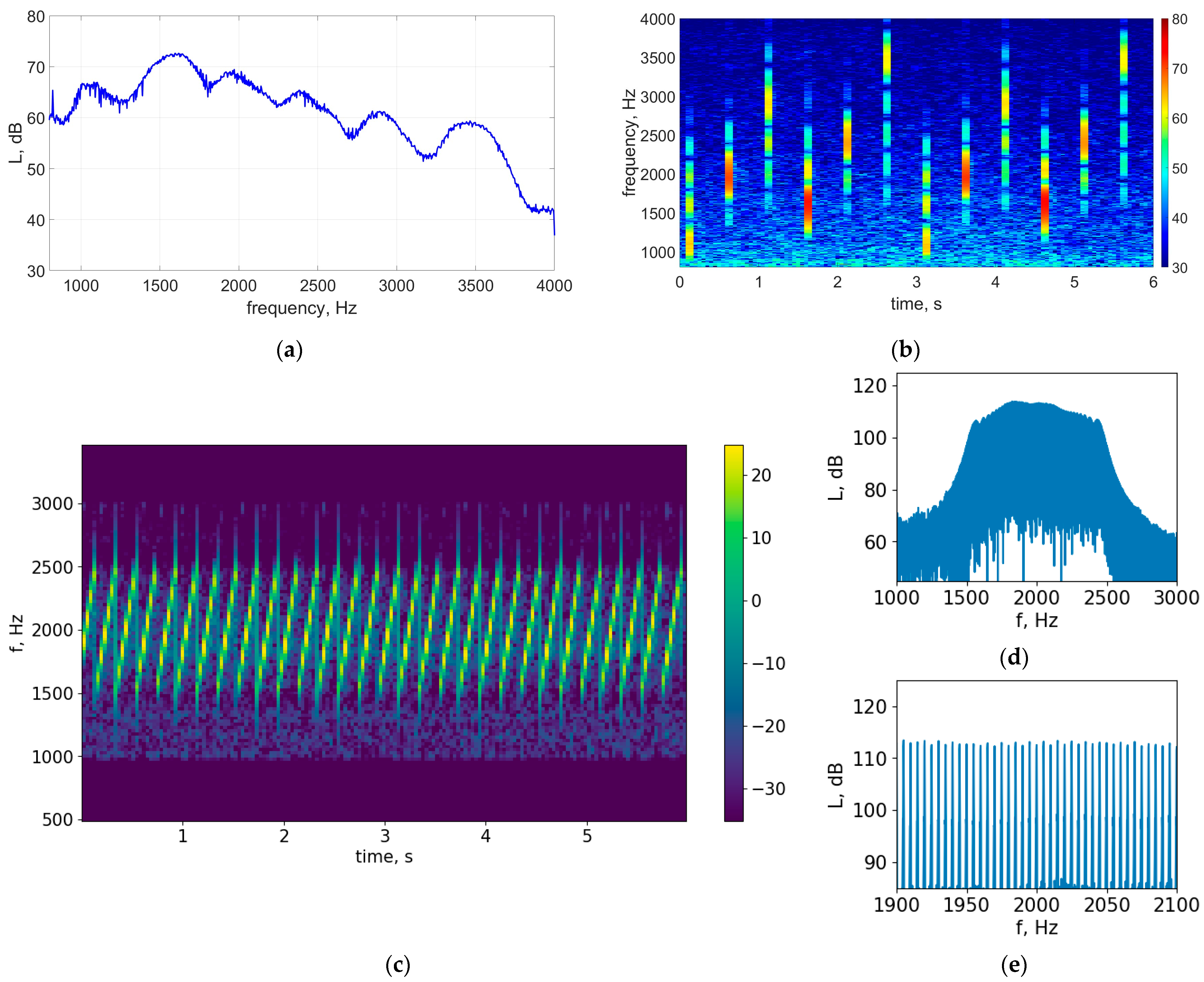
3.3. Narrowband Analysis of Surface Reverberation

Let us consider in more detail the moments of reflection from the surface and calculate the narrowband spectrum at these moments of time. In order for the uncertainty function of the probing signal to correspond to the desired Doppler frequency resolution, we will turn to the radiation mode in the form of PTFM [34,35]. Due to the strict periodicity (Figure 3c), the signal has a comb-like spectrum (Figure 3e). The frequency resolution is determined by the total duration of the packet and in this case is 0.16 Hz. The shift relative to the central frequency can be determined within ±2.5 Hz, which is the Nyquist frequency relative to the pulse repetition period in the packet. The time resolution is determined by the total bandwidth; here, it is 1 ms or 75 cm for the signal round trip. The interval of unambiguously measurable arrival times is limited by the “distance between adjacent saw teeth”—up to 0.2 s, which corresponds to 150 m. The sound-scattering phenomena studied in the experiment fit within these limitations.

Figure 10 shows the signal spectra for the selected angle and delay time corresponding to the most interesting points in Figure 8. The top row shows the results for station 1, and the bottom row shows the results for station 2. The left column shows the spectra of the signals that passed along the bottom paths: the maxima b, e in Figure 8 correspond to the solid and dashed lines in Figure 10a,d. The middle column shows the spectra of the signals reflected from the surface: the maxima c, d in Figure 8 correspond to the solid and dashed lines in Figure 10b,e. The right column shows the scattering on the surface at oblique angles (not specular reflection): for a ray arriving at an angle of $\phi =70°$ to the vertical, the corresponding delay is determined along the lines c, d in Figure 8 and the spectra are calculated for these coordinates (angle, delay), then plotted by the solid and dashed lines in Figure 10c,f (in Figure 10c, the lines merge and only one of them is plotted). Due to the finite resolution of the receiving system and the bistatic geometry of the experiment, in the latter case the response was formed by waves incident on the surface at angles $\alpha$ in the range from ~12 to ~30$°$ to the vertical. The plotted spectra graphs are compared with theoretical or reference dependencies (colored dots, which are plotted in the same axes with level correction to match the maxima of the experimental curves).

We are interested in the width of the experimentally obtained spectra, since it determines the stability of a particular sound propagation path, which, for example, affects the possibility of transmitting information along it. For bottom rays, the spectrum of the signal transmitted along the shortest path from the source to the receiver without distortion is constructed in the same axes (see the colored dotted line (dot) in Figure 10a,d). In this case, this is a reference dependence, since we believe that reflection from the bottom, as from a stationary scatterer, does not lead to a change in the shape of the spectrum. Further, it is clear that all cases when the rays touch the rough surface are associated with a broadening of the spectrum due to the Doppler effect. Due to the multidirectional and multi-scale motion of the sea surface, determining the shape of the spectrum of the reflected signal is possible only by numerical modeling methods. Based on the nonlinear hydrodynamic model, a dynamically changing shape of the free surface was generated for the sea states close to the experimental conditions [36,37]. After this, the calculation of sound reflection and scattering was performed using the boundary element method [27] for specific angles of incidence and scattering of the wave, which were determined from the ray model developed above. The results of the modeling are plotted in Figure 10b,c,e,f using the colored dotted lines. All reference dependencies are level-corrected to match the maxima of the solid curves. It is important to note that, when acoustic scattering on such a surface as that on which a realistic air–water boundary is simulated, it results in an estimation of scattering strength per unit length. It cannot be compared directly to the experimental data, as the real-life scattering strength is normalized per unit area. That is the reason for introducing level correction, and this procedure is needed only when we present Doppler spectra (Figure 10). When a simpler model is exploited for surface scattering strength, like Chapman–Harris, then we compute in 3D and no special level correction is applied (Figure 8).

The experiments at the two stations under study were conducted under different sea state conditions: the experiment at station 1 (top row in Figure 10) was conducted under a rippled sea state and wind speed of about 5 m/s, while at station 2 (bottom row in Figure 10), it was conducted under a rough sea state and wind speed of over 10 m/s. The difference in sea state can be seen in the surface reverberation spectra: first of all, one can pay attention to the width of the spectrum of the signal reflected from the surface: in the case of a rippled sea state in Figure 10b, the maximum of the signal spectrum is preserved at the central frequency, but in the case of rough sea state in Figure 10e, “chaos” is observed and the energy is evenly distributed over the entire measured frequency range.

Of particular interest is the study of scattering at oblique angles (not specular reflection). The consideration of this case is interesting because the operation of sonars in marine conditions will encounter this type of scattering, but at even more shallow angles of incidence [4,22]. Figure 10c demonstrates the occurrence of a Bragg side lobe at the frequency:

$$Fdop=\sqrt{{\displaystyle \frac{\overline{f}g\mathrm{s}\mathrm{i}\mathrm{n}\alpha }{\pi c}}},$$

(11)

where $\overline{f}$ is the average frequency of the chirp signal and $g$ is the acceleration due to gravity. This effect was known theoretically earlier, but is rarely observed directly in acoustics [38]. In this case, zero Doppler frequency recorded into the spectrum is, apparently, an inevitable experimental error. The Bragg peak has a Gaussian shape around the frequency (11). The broadening of the Bragg peak is associated with 3-D effects, with the non-monochromaticity of the signal and, mainly, with the nonlinear interaction in the wave field, when short waves are modulated by long ones. An asymmetry of this kind, when only positive Doppler frequencies are observed, is a matter of chance. Here, it is apparently associated with the asymmetry of the experiment; for example, part of the sea surface on which the sound could be scattered could be blocked by the side of the ship.

In the case of strong waves, as observed at station 2, the scattering pattern at oblique angles changes dramatically. The scattered field energy is distributed over Doppler frequencies as a Gaussian function centered at zero frequency (Figure 10f). This is a consequence of the complex interaction at the water–air interface and the resulting bubble suspension [13].

Overall, the graphs show that the theory reproduces the effects observed in the experiment. Mostly, the correct tendency for the Doppler spectrum width to increase with increasing waves is modeled. The discrepancy between the modeling and experimental results can be explained by the limitations of the two-dimensional model and the inaccuracy of the wave spectrum specification at the modeling input.

4. Conclusions

The method for experimental studies of surface waves and seabed characteristics using mid-range underwater acoustics has been developed. The experiment can be conducted from a research vessel with a limited source and receiver separation distance. This approach makes acoustic studies in various areas more accessible.

The method proposed has been successfully applied in experimental studies in the Barents and Kara Seas. Significant heterogeneity of the acoustic energy transmission coefficient into bottom sediments at various points in these seas has been demonstrated. A significant difference in the Doppler spectra of signals scattered on the surface under various wave conditions has been indicated.

An original set of methods and approximations was applied to the algorithm for modeling reverberation.

An original set of methods and approximations for numerical modeling of reverberation in shallow-water shelf conditions has been developed to interpret the experimental results, combining the ray method for calculating sound propagation and a local model of sound scattering on uneven surfaces. The theory and experiment agree satisfactorily.

At this stage, a qualitative assessment of the model’s performance with the available data was performed. Model improvement, as well as an assessment of its accuracy, will be carried out in future studies.

References

1. Mirza, J.; Kanwal, F.; Salaria, U.A.; Ghafoor, S.; Aziz, I.; Atieh, A.; Almogren, A.; Haq, A.U.; Kanwal, B. Underwater temperature and pressure monitoring for deep-sea SCUBA divers using optical techniques. Sec. Opt. Photonics 2024, 12, 1417293. [Google Scholar] [CrossRef]
2. Joshi, B.; Xanthidis, M.; Roznere, M.; Burgdorfer, N.J.; Mordohai, P.; Li, A.Q.; Rekleitis, I. Underwater Exploration and Mapping. In Proceedings of the IEEE/OES Autonomous Underwater Vehicles Symposium (AUV), Singapore, 19–21 September 2022; pp. 1–7. [Google Scholar] [CrossRef]
3. Charkin, A.N.; Kosobokova, K.N.; Ershova, E.A.; Syomin, V.L.; Kolbasova, G.D.; Semkin, P.Y.; Leusov, A.E.; Dudarev, O.V.; Gulenko, T.A.; Yaroshchuk, E.I.; et al. A unique warm–water oasis in the Siberian Arctic’s Chaun Bay sustained by hydrothermal groundwater discharge. Commun. Earth Environ. 2024, 5, 393. [Google Scholar] [CrossRef]
4. Bjørnø, L. Chapter 5—Scattering of Sound. In Applied Underwater Acoustics; Neighbors, T.H., Bradley, D., Eds.; Elsevier: Amsterdam, The Netherlands, 2017; pp. 297–362. [Google Scholar] [CrossRef]
5. Malekhanov, A.I.; Smirnov, I.P. Array acoustic signal processing in shallow-water channels under conditions of a priori uncertainty: Estimates of the efficiency loss. Acoust. Phys. 2022, 68, 382–394. [Google Scholar] [CrossRef]
6. Li, P.; Wu, Y.; Guo, W.; Cao, C.; Ma, Y.; Li, L.; Leng, H.; Zhou, A.; Song, J. Striation-Based Beamforming with Two-Dimensional Filtering for Suppressing Tonal Interference. J. Mar. Sci. Eng. 2023, 11, 2117. [Google Scholar] [CrossRef]
7. Dmitrieva, D.; Romasheva, N. Sustainable Development of Oil and Gas Potential of the Arctic and Its Shelf Zone: The Role of Innovations. J. Mar. Sci. Eng. 2020, 8, 1003. [Google Scholar] [CrossRef]
8. Krylov, A.A.; Ananiev, R.A.; Chernykh, D.V.; Alekseev, D.A.; Balikhin, E.I.; Dmitrevsky, N.N.; Novikov, M.A.; Radiuk, E.A.; Domaniuk, A.V.; Kovachev, S.A.; et al. A Complex of Marine Geophysical Methods for Studying Gas Emission Process on the Arctic Shelf. Sensors 2023, 23, 3872. [Google Scholar] [CrossRef]
9. Li, Z.; Yang, Y.; Wen, H.; Zhou, H.; Ruan, H.; Zhang, Y. The Extraction and Validation of Low-Frequency Wind-Generated Noise Source Levels in the Chukchi Plateau. J. Mar. Sci. Eng. 2025, 13, 49. [Google Scholar] [CrossRef]
10. Brekhovskikh, L.M.; Godin, O.A. Acoustics of Layered Media I. Plane and Quasi-Plane Waves; Springer Series on Wave Phenomena; Springer: Berlin, Germany, 1990; Volume 5, 240p, ISBN 3-540-51038-9. [Google Scholar]
11. Jensen, F.B.; Kuperman, W.A.; Porter, M.B.; Schmidt, H. Computational Ocean Acoustics; Springer: New York, NY, USA, 2011. [Google Scholar]
12. Hassantabar Bozroudi, S.H.; Ciani, D.; Mohammad Mahdizadeh, M.; Akbarinasab, M.; Aguiar, A.C.B.; Peliz, A.; Chapron, B.; Fablet, R.; Carton, X. Effect of Subsurface Mediterranean Water Eddies on Sound Propagation Using ROMS Output and the Bellhop Model. Water 2021, 13, 3617. [Google Scholar] [CrossRef]
13. Salin, M.B.; Ermoshkin, A.V.; Razumov, D.D.; Salin, B.M. Models of the formation of Doppler spectrum of surface reverberation for sound waves of the meter range. Acoust. Phys. 2023, 69, 687–698. [Google Scholar] [CrossRef]
14. Isakson, M.J.; Chotiros, N.P. Finite element modeling of acoustic scattering from fluid and elastic rough interfaces. IEEE J. Ocean. Eng. 2015, 40, 475–484. [Google Scholar] [CrossRef]
15. Ellis, D.D. Modelling Bottom Scattering and Target Echoes from Data Collected During the 2013 Target and Reverberation Experiment. In Proceedings of the UACE2017—4th Underwater Acoustics Conference and Exhibition, Skiathos, Greece, 3–8 September 2017; pp. 245–252. [Google Scholar]
16. Tang, D.; Hefner, B.T.; Jackson, D.R. Direct-Path Backscatter Measurements Along the Main Reverberation Track of TREX13. IEEE J. Ocean. Eng. 2019, 44, 983. [Google Scholar] [CrossRef]
17. Lunkov, A.A. Interference structure of low-frequency reverberation signals in shallow sea. Acoust. J. 2015, 61, 596–604. (In Russian) [Google Scholar] [CrossRef]
18. Jenserud, T.; Ivansson, S. Measurements modeling of effects of out-of-plane reverberation on the power delay profile for underwater acoustic channels. IEEE J. Ocean. Eng. 2015, 40, 807–821. [Google Scholar] [CrossRef]
19. Jung, Y.; Lee, K. Observation of the Relationship between Ocean Bathymetry and Acoustic Bearing-Time Record Patterns Acquired during a Reverberation Experiment in the Southwestern Continental Margin of the Ulleung Basin, Korea. J. Mar. Sci. Eng. 2021, 9, 1259. [Google Scholar] [CrossRef]
20. Jung, Y.; Seong, W.; Lee, K.; Kim, S. A Depth-Bistatic Bottom Reverberation Model and Comparison with Data from an Active Triplet Towed Array Experiment. Appl. Sci. 2020, 10, 3080. [Google Scholar] [CrossRef]
21. Isakson, M.J.; Chotiros, N.P. Finite element modeling of reverberation and transmission loss in shallow water waveguides with rough boundaries. J. Acoust. Soc. Am. 2011, 129, 1273–1279. [Google Scholar] [CrossRef]
22. Urick, R.J. Principles of Underwater Sound; McGraw-Hill: New York, NY, USA, 1975. [Google Scholar]
23. Samchenko, A.; Dolgikh, G.; Yaroshchuk, I.; Korotchenko, R.; Kosheleva, A. Geoacoustic Digital Model for the Sea of Japan Shelf (Peter the Great Bay). Geosciences 2024, 14, 288. [Google Scholar] [CrossRef]
24. Sidorov, D.D.; Petnikov, V.G.; Lunkov, A.A. Broadband sound field in a shallow-water waveguide with a non-uniform bottom. Acoust. J. 2023, 69, 608–619. (In Russian) [Google Scholar] [CrossRef]
25. Trzcinska, K.; Tegowski, J.; Pocwiardowski, P.; Janowski, L.; Zdroik, J.; Kruss, A.; Rucinska, M.; Lubniewski, Z.; Schneider von Deimling, J. Measurement of Seafloor Acoustic Backscatter Angular Dependence at 150 kHz Using a Multibeam Echosounder. Remote Sens. 2021, 13, 4771. [Google Scholar] [CrossRef]
26. Hartstra, I.; Colin, M.; Prior, M. Active sonar performance modelling for Doppler-sensitive pulses. Proc. Meet. Acoust. 2021, 44, 022001. [Google Scholar] [CrossRef]
27. Kalinina, V.I.; Vyugin, P.N.; Kapustin, I.A. Physical modeling of the method of coherent probing of low-contrast bottom layers in a laboratory pool. Acoust. Phys. 2024, 70, 536–550. [Google Scholar] [CrossRef]
28. Salin, M.; Razumov, D. Multi-domain boundary element method for sound scattering on a partly perturbed water surface. J. Theor. Comput. Acoust. 2020, 28, 2050006. [Google Scholar] [CrossRef]
29. Purdon, J. Calming the Waves: Using Legislation to Protect Marine Life from Seismic Surveys; South African Institute of International Affairs Policy Insights: Johannesburg, South Africa, 2018; Volume 58. [Google Scholar]
30. Zuikova, E.M.; Baydakov, G.A.; Titchenko, Y.A.; Salin, M.B. 3 cm Doppler scatterometer with full polarization sensing. J. Radio Electron. 2021, 2021, 1–22. [Google Scholar] [CrossRef]
31. Liu, Z.; Tao, Q.; Sun, W.; Fu, X. Deconvolved Fractional Fourier Domain Beamforming for Linear Frequency Modulation Signals. Sensors 2023, 23, 3511. [Google Scholar] [CrossRef]
32. Ellis, D.D.; Crowe, D.V. Bistatic reverberation calculations using a three-dimensional scattering function. J. Acoust. Soc. Am. 1991, 89, 2207–2214. [Google Scholar] [CrossRef]
33. Andreeva, I.B. Comparative assessments of surface, bottom and volume scattering of sound in the ocean. Acoust. J. 1995, 41, 699–705. Available online: http://www.akzh.ru/pdf/1995_5_699-705.pdf (accessed on 1 June 2025). (In Russian).
34. Guo, R.; Wang, X.; Cai, Z. Comparison research on reverberation strength excited by PTFM and CW signals. In Proceedings of the IEEE 13th International Conference on Signal Processing (ICSP), Chengdu, China, 6–10 November 2016; pp. 1677–1681. [Google Scholar] [CrossRef]
35. Guan, C.; Zhou, Z.; Zeng, X. Optimal waveform design using frequency-modulated pulse trains for active sonar. Sensors 2019, 19, 4262. [Google Scholar] [CrossRef]
36. Ermoshkin, A.V.; Dosaev, A.S.; Razumov, D.D.; Tsvetkov, K.A.; Salin, M.B. Manifestation of the nonlinearity of wind waves in coherent remote sensing signals. Radiophys. Quantum Electron. 2025. in print. [Google Scholar]
37. Baidakov, G.A.; Dosaev, A.S.; Razumov, D.D.; Salin, M.B. Estimation of broadening of the spectra of short surface waves in the presence of long waves. Radiophys. Quantum Electron. 2018, 61, 332–341. [Google Scholar] [CrossRef]
38. Salin, M.B.; Potapov, O.A.; Salin, B.M.; Chashchin, A.S. Measuring the characteristics of backscattering of sound on a rough surface in the near-field zone of a phased array. Acoust. Phys. 2016, 62, 74–88. [Google Scholar] [CrossRef]
Figure 1. A map of the research area with the location of the stations at which hydroacoustic measurements were carried out.
Jmse 13 01122 g001
Figure 2. Experiment scheme.
Jmse 13 01122 g002
Figure 3. Spectra of probing signals; tone pulses (a,b); chirp signal (ce).
Jmse 13 01122 g003
Figure 4. Sound speed profile: (a) at station 1; (b) at station 2. The black dots show the location of the sound source, the red ones show the position of the center of the receiving antenna.
Jmse 13 01122 g004
Figure 5. A scheme of the method of stepwise approximation of the profile of the dependence of sound speed on the depth (a) and rays (b) taken into account in the numerical model (the colors show the different directions of the rays).
Jmse 13 01122 g005
Figure 6. The separation of rays into groups. The numbers indicate different groups of rays. The color scale corresponds to the logarithm of the amplitude.
Jmse 13 01122 g006
Figure 7. The level of the received signal as a function of time for different viewing angles for station 1 (I) and station 2 (II). The red curve corresponds to the direct signal, the black dotted line is the signal received from angles directed towards the surface, and the blue dotted line is the signal received from angles directed to the bottom. Designations in the figure: “a”—direct signal; “b”—single reflection from the bottom; “c”—reflection from the surface; multiple reflections: “d”—bottom–surface; “e”—surface–bottom; “f”—bottom–surface–bottom; “g”—surface–bottom–surface; “h”—reflections of higher orders.
Jmse 13 01122 g007
Figure 8. Result of processing experimental data from station 1 (I) and station 2 (II). Designations in the figure: “a”—direct signal; “b”—single reflection from the bottom; “c”—reflection from the surface; multiple reflections: “d”—bottom–surface; “e”—surface–bottom; “f”—bottom–surface–bottom; “g”—surface–bottom–surface; “h”—reflections of higher orders; “i”—signal reflected from the ship hull; “j”—noise signal from the ship engine, observed from angles of 70–90°. The color of the circles corresponds to the scale of the main graph and shows the signal level in dB.
Jmse 13 01122 g008
Figure 9. The level of losses in the bottom depending on the frequency of the sounding signal and for different stations; the blue dotted line is a depth graph for these stations.
Jmse 13 01122 g009
Figure 10. Doppler spectra of reflected signals obtained: (ac) from station 1 and (df) from station 2 data together with numerical modeling. Solid and dotted black lines (dash) and green dots (dots) are experimental spectra obtained along different propagation paths in accordance with the attached schemas; cyan dots are the results of numerical modeling. Levels are given in dB relative to the conventional unit; the noise level corresponds to approximately 50 dB in these units.
Jmse 13 01122 g010
Disclaimer/Publisher’s Note: The statements, opinions and data contained in all publications are solely those of the individual author(s) and contributor(s) and not of MDPI and/or the editor(s). MDPI and/or the editor(s) disclaim responsibility for any injury to people or property resulting from any ideas, methods, instructions or products referred to in the content.