Analysis of Wind–Wave Relationship in Taiwan Waters

Abstract

The relationship between wind and waves has been extensively studied over time. However, understanding the local wind and wave relationship remains crucial for advancing renewable energy development and optimizing ocean management strategies. This study used wind and wave data collected by the ten weather buoys in the waters surrounding Taiwan to analyze regional sea states. The relationship between wind speed and significant wave height (SWH) was examined using regression analysis. Additionally, machine learning techniques were employed to assess the relative importance of features contributing to SWH growth. The regression analysis revealed that SWH in the waters surrounding Taiwan was not fully developed, with notable discrepancies observed between the waters east and west of Taiwan. According to the power law formula describing the relationship between wind speed and SWH, the eastern waters exhibited a larger prefactor coupled with a smaller scaling exponent, while the western waters manifested a converse parametric configuration. Through an evaluation of four machine learning algorithms, it was determined that wind speed is the most influential factor driving these regional differences, especially in the waters west of Taiwan. Beyond wind speed, air pressure or temperature emerged as the secondary feature factor governing wind–wave interactions in the waters east of Taiwan.

1. Introduction

Waves and winds within the lower marine atmospheric boundary layer are crucial components of air–sea interactions, significantly influencing weather patterns and climate systems. A primary focus of research in this field is the relationship between wind and waves, which plays a pivotal role in processes such as momentum transfer, heat flux, and mass exchange. Despite decades of study, this relationship remains complex due to factors like wind intensity, fetch, water depth, and the presence of currents or swell, presenting significant scientific challenges [1].

Significant wave height (SWH), denoted as H_S, is defined as the mean wave height of the highest one-third of waves. It serves as a statistical measure indicative of the overall sea state. This parameter is essential for understanding oceanic conditions and informs engineering decisions regarding maritime structures and operations. Accurate prediction and monitoring of SWH are crucial for ensuring safety and efficiency in maritime activities, such as shipping, fishing, and offshore engineering, as elevated wave heights pose substantial risks to vessels and offshore installations [2,3]. In ocean engineering, SWH is a fundamental consideration for designing structures such as piers, harbors, and offshore platforms. Engineers utilize SWH data to assess potential loads and stresses on these structures to ensure their resilience against extreme conditions, including severe weather events [4,5]. Additionally, SWH is integral to physical oceanography, aiding researchers in understanding wave dynamics and their interactions with wind, currents, and other environmental factors. Insights gained from SWH data are critical for studying climate change impacts on ocean behavior and modeling coastal erosion processes [3,6]. Statistically, wave heights typically follow a Rayleigh distribution, with SWH serving as a reference point for estimating the probability of encountering larger waves.

Recent advancements introduced artificial intelligence (AI) techniques, such as long short-term memory (LSTM) networks and random forests (RFs), as powerful tools for predicting wind-induced waves. These methods have demonstrated effectiveness in forecasting SWH across various temporal scales by capturing dynamic interactions between wind conditions and wave heights [7,8,9]. Compared to conventional numerical models, AI approaches can enhance prediction accuracy while reducing computational demands, making them valuable for marine engineering and offshore operations [10]. However, challenges persist in integrating physical knowledge into AI models and validating their performance across diverse oceanic environments.

Taiwan’s geographic location further underscores the importance of studying wind–wave interactions. Situated in East Asia on the southwest side of the North Pacific Ocean, Taiwan is bordered by the East China Sea to the north, the Pacific Ocean to the east, the Taiwan Strait to the west, and the Luzon Strait to the south. The island spans approximately 400 km in length with a maximum width of 150 km. Taiwan’s tropical and subtropical climates are heavily influenced by the East Asian monsoon, resulting in distinct rainy and dry seasons. The northeast monsoon, which dominates from October to April, brings strong winds averaging 11–12 m/s, while the southwest monsoon from May to September exhibits lower wind speeds [11,12]. These seasonal wind patterns, combined with Taiwan’s maritime surroundings, create a dynamic wave climate that is crucial for renewable energy development, climate adaptation, coastal safety, disaster preparedness, and marine ecosystem management.

Given its strong and consistent winds, especially in the Taiwan Strait, Taiwan is an ideal site for offshore wind energy generation. Seasonal monsoons, climate variability, and climate change further influence Taiwan’s wave climate [13,14,15,16,17,18], necessitating robust monitoring of wave conditions to improve preparedness for extreme weather events, such as typhoons, and to support coastal protection strategies.

Future projections suggest that climate change will substantially alter wave climates around Taiwan, with significant implications for coastal erosion, sediment transport, and marine ecosystems. Understanding wind–wave interactions is therefore vital for developing effective strategies to protect coastlines, manage fisheries, and conserve biodiversity.

Despite extensive research, significant knowledge gaps remain—particularly regarding the differences in wind and wave relationships between the eastern and western waters of Taiwan, which are influenced by distinct topographic and environmental conditions. This study aims to address these gaps by utilizing high-quality observational data to enhance the understanding of wind-induced waves around Taiwan, ultimately providing information to support sustainable maritime practices.

2. Materials and Methods

2.1. Materials

The wind and wave data utilized in this study were obtained from weather buoys deployed in Taiwan’s waters. These buoys collect data at a frequency of 2 Hz for 10 min every hour, measuring multiple parameters, including waves, sea surface winds at heights of 2 and 3 m, currents, sea temperature, air temperature, and air pressure. To ensure the reliability of the measurements, a rigorous data quality control system was implemented [19]. The dataset is accessible via the “SafeOcean” platform (https://ocean.cwa.gov.tw/V2/taiwan_marine, accessed on 11 January 2025) and provides valuable insights into wind–wave interactions, climate variability, and trends. A total of 16 weather buoys have been deployed by Taiwan’s Central Weather Administration across Taiwan’s waters. However, due to interruptions in data collection or incomplete measurements from some buoys, this study focused on data from ten buoys with relatively complete records. Figure 1 illustrates the deployment locations of these buoys, and

Table 1. Information on weather buoys used in this study.

Buoy	Latitude (°N)	Longitude (°E)	Water Depth (m)	Distance to Coast (Km)	Date of Data Available
Longdong	25.098610	121.922770	27	0.5	1998–2025
Guishandao	24.848300	121.926100	19	0.8	2002–2024
Hualien	24.031500	121.632300	24	0.4	1997–2025
Lanyu	22.069720	121.579160	50	1	2017–2024
Matsu	26.354440	120.510830	52	2.7	2010–2025
Fuguijiao	25.303880	121.532770	30	0.8	2015–2025
Hsinchu	24.763300	120.844100	24.5	6.4	1997–2025
Qimei	23.188880	119.665000	50	22.8	2015–2025
Taichung	24.239400	120.413300	18.5	11	2019–2025
Dongshadao	21.055600	118.853300	2550	224	2010–2024

provides detailed information about their specifications. Of these ten buoys, four are situated in Taiwan’s western waters and six in its eastern waters. The study period spans from 2020 to 2024 to ensure consistency across buoy stations.

A data buoy is an autonomous floating platform with sensors that record oceanographic and meteorological conditions. To measure the wave parameters, the data buoy is equipped with a 3-axis accelerometer and gyroscope to measure the passing ocean waves. The accelerometer records acceleration along the vertical (heave), longitudinal (surge), and lateral (sway) axes, while the gyroscope captures angular velocity associated with pitch, roll, and yaw. The directional wave spectrum $S\left(f,\theta \right)$ is derived to estimate the wave parameters, where f is the frequency and θ is the angle. It describes how wave energy is distributed across different frequencies and propagation directions, providing a comprehensive view of the sea state’s structure. Many methods have been developed to derive the directional wave spectra, such as the finite Fourier series method [20], the maximum entropy method [21], the maximum likelihood method [22], and the Bayesian directional estimation [23]. The data buoy deployed in Taiwan’s waters uses the finite Fourier series method to derive the directional wave spectrum. The total wave energy ($m_0$) is obtained by performing a double integration of the directional wave spectrum over frequency and direction using Equation (1) [24,25].

$$m_i={\int }_0^{\infty }{f}^{i}S\left(f,\theta \right)dfd\theta$$

(1)

where $m_i$ is the spectral moment of order i. The SWH is then estimated using the zeroth spectral moment as

$$H_s=4.0\sqrt{m_0}.$$

(2)

The significant wave period is calculated from spectral moments as well. The significant wave period ($T_s$) is the root of the ratio of zeroth with second moments as shown in Equation (3)

$$T_s=\sqrt{{\displaystyle \frac{m_0}{m_2}}}.$$

(3)

The data collected by these buoys are instrumental in advancing research on wind–wave relationships and their variability over time. They also contribute to understanding climate trends and variability, supporting applications, such as renewable energy development, coastal safety, disaster preparedness, and marine ecosystem management.

2.2. Methods

2.2.1. Distinguishing Between Wind Waves and Swells

SWH at a given local wind speed ($U$) comprises two components: swell SWH propagating from open seas and locally generated SWH influenced by immediate wind conditions. Isolating swell SWH is critical for assessing local wind impacts on wave dynamics. While probabilistic frameworks have been proposed to differentiate swell from wind-driven SWH [26], a simplified approach leverages the distinct morphological characteristics of these wave types. The separation of wind wave and swell contributions in the SWH is typically achieved through spectral partitioning of the wave energy spectrum. Wind waves generally appear at higher frequencies and are closely aligned with the local wind direction, while swells appear at lower frequencies, often originating from distant sources and exhibiting a broader directional spread [27].

Wind-generated waves typically exhibit shorter periods (<10 s) compared to swell, as empirically established by spectral analyses [28,29,30,31]. This temporal distinction forms the basis for a widely adopted classification threshold, where waves with periods exceeding 10 s are categorized as swells [28]. Furthermore, propagation direction serves as a secondary discriminator: wind waves predominantly align with local wind vectors, whereas swells may originate from divergent directional sources [32,33]. Previous studies suggested that wind waves typically have the wind–wave alignment less than 45° [34] or 60° [35]. Thus, this study operationalizes these principles by classifying wave types using two criteria as (1) temporal separation: wind waves are defined by periods <10 s, and (2) angular divergence: waves propagating within ±45° of wind direction are classified as wind waves.

2.2.2. Regression

The relationship between local wind speed and wave height is often described using a power-law formula. In contemporary studies, wave characteristics are typically expressed in terms of SWH and wind speed (denoted as $U_{10}$) measured at a standard height of 10 m. This relationship can be mathematically formulated as follows [36]:

$$H_s=\mathrm{\alpha }{U}_{10}^{\beta },$$

(4)

where α represents the prefactor and β denotes the scaling exponent. The value of β is influenced by the sea state during measurement. For a fully developed sea, β is conventionally equal to 2 [26,36]. However, deviations from this quadratic relationship have been observed under specific conditions. For instance, a study [26] has reported a scaling exponent of β = 1.62 ± 0.15 for high wind speeds, suggesting that alternative power-law exponents may better capture the dynamics in certain scenarios. These deviations highlight that the wind–wave relationship is not solely determined by sea state but is also affected by additional factors such as water depth [37] and temperature variations [18]. To estimate the parameters α and β, Equation (4) is logarithmically transformed, enabling the application of linear regression techniques to derive optimal solutions.

2.2.3. Calculation of Wind Speed at 10 m Height

Wind measurements at weather buoys are recorded at heights of 2 m and 3 m above the sea surface. To extrapolate wind velocity to the standard 10 m height ($U_{10}$), this study employs the surface wind profile equation under neutral atmospheric stability conditions [26,38]:

$$U_z={\displaystyle \frac{u_{*}}{\kappa }}\mathrm{l}\mathrm{n}{\displaystyle \frac{z}{z_0}},$$

(5)

where κ is the von Kármán constant, z₀ denotes the roughness length, z represents the measurement height above the sea surface, and $u_{*}$ is the friction velocity. The $u_{*}$ can be experimentally determined from $U_{10}$ and the drag coefficient $C_d$ as follows [39]:

$$u_{*}=\sqrt{C_d}{U}_{10}.$$

(6)

Substituting Equation (6) into Equation (5) yields [38]

$$U_{10}=U_z\sqrt{{\displaystyle \frac{{\kappa }^2}{C_d}}}{\displaystyle \frac{1}{ln\left(z/z_0\right)}}.$$

(7)

Standard parameters from the literature were adopted: κ = 0.4, z₀ = 9.7 × 10⁻⁵, and $C_d$ = 1.2 × 10⁻³ [26]. However, for neutral air stratification, $C_d$ is unambiguously associated with $z_0$; therefore, $U_{10}$ can be calculated directly as

$$U_{10}={\displaystyle \frac{U_z}{1+\frac{\sqrt{C_d}}{\kappa }\ln \left(\frac{z}{10}\right)}}.$$

(8)

Using Equation (8), wind speeds measured at 2 m (z = 2) and 3 m (z = 3) heights were extrapolated to $U_{10}$. Results from both heights showed negligible differences, confirming the robustness of the method. Consequently, this study utilized wind speed measurements at the 2 m height for $U_{10}$ calculations.

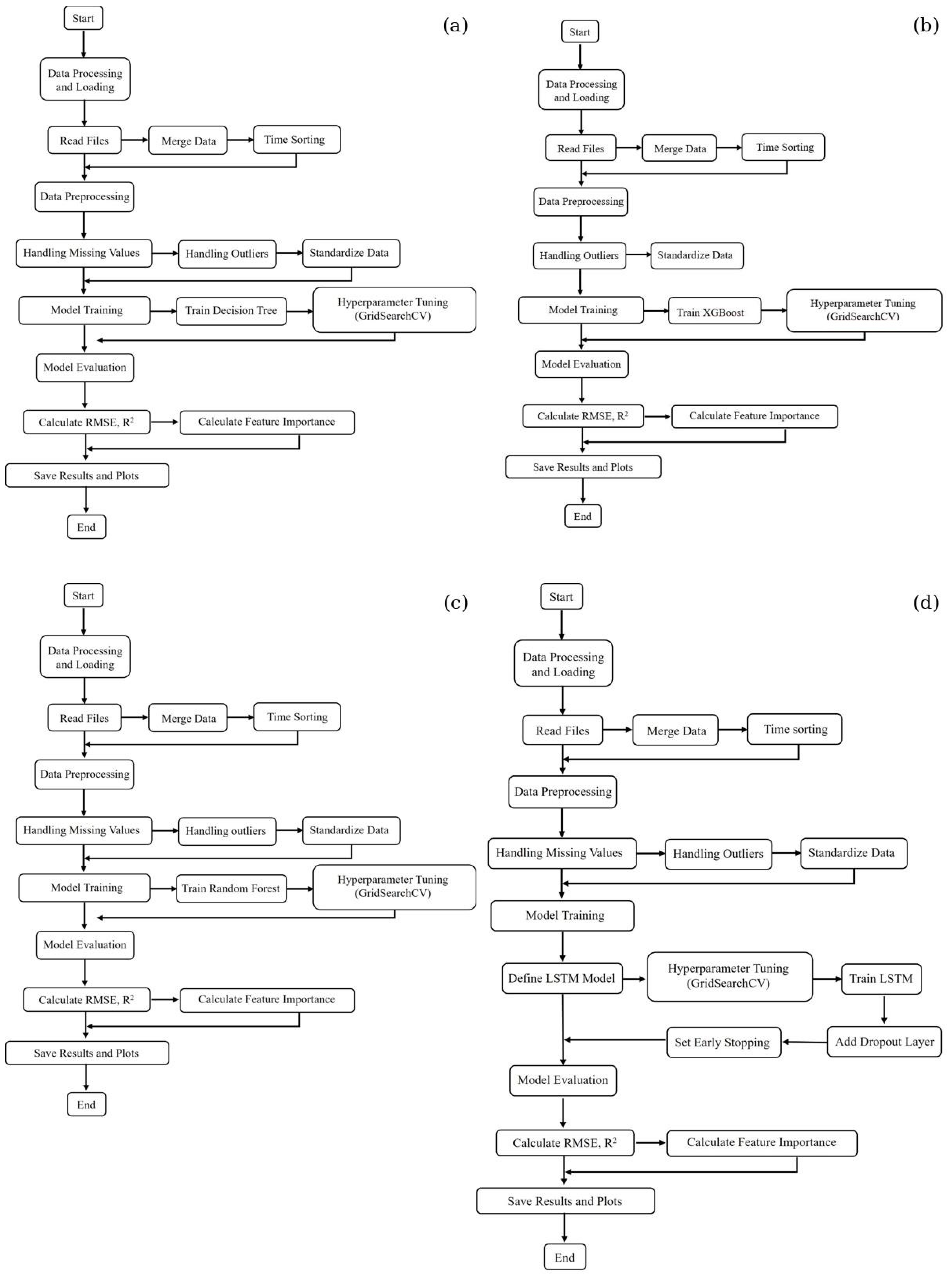
2.2.4. Machine Learning Methods

AI methods have been increasingly employed to predict SWHs using wind data as input [8] and some AI algorithms can also examine feature importance to provide insights into the factors that affect the prediction. To validate the wind–wave relationships derived through regression methods, this study integrates AI-based approaches, including decision trees (DTs), extreme gradient boosting (XGBT), RF, and LSTM, to investigate the relationship between wind and waves.

DT is a supervised machine learning algorithm used for classification and regression tasks. It operates by splitting data into subsets based on decision rules derived from input features, creating a hierarchical tree structure. It performs decision-making processes through the hierarchical tree structure, where internal nodes correspond to features, branches denote feature values and leaf nodes indicate predicted outcomes [40,41]. XGBT is a machine learning algorithm based on gradient boosting, designed for supervised learning tasks such as classification and regression [42], XGBT builds decision trees sequentially, where each tree focuses on correcting the residuals (errors) of the previous model. It uses gradient descent to optimize a loss function and incorporates second-order Taylor approximations for faster convergence. The algorithm adjusts weights for incorrectly predicted samples, making subsequent trees more accurate. This iterative process results in a robust ensemble model that performs well across various domains. RF is another supervised machine learning algorithm that creates an ensemble of multiple decision trees to solve classification and regression problems. It is based on the concept of ensemble learning, where multiple models are combined to improve predictive accuracy and reduce overfitting. Each decision tree in the forest is trained on a random subset of the data, and predictions are aggregated using either majority voting (for classification) or averaging (for regression) [43,44,45]. LSTM networks are specialized recurrent neural networks designed to learn long-term dependencies effectively while addressing challenges such as the vanishing gradient problem inherent in traditional recurrent neural networks. They are particularly suited for time-series data analysis and prediction tasks [46,47,48,49].

By employing these AI algorithms, this study aims to refine our understanding of wind–wave interactions while leveraging their predictive capabilities. The integration of machine learning methods not only enhances prediction accuracy but also facilitates deeper insights into the dynamics governing wind-induced waves.

3. Results

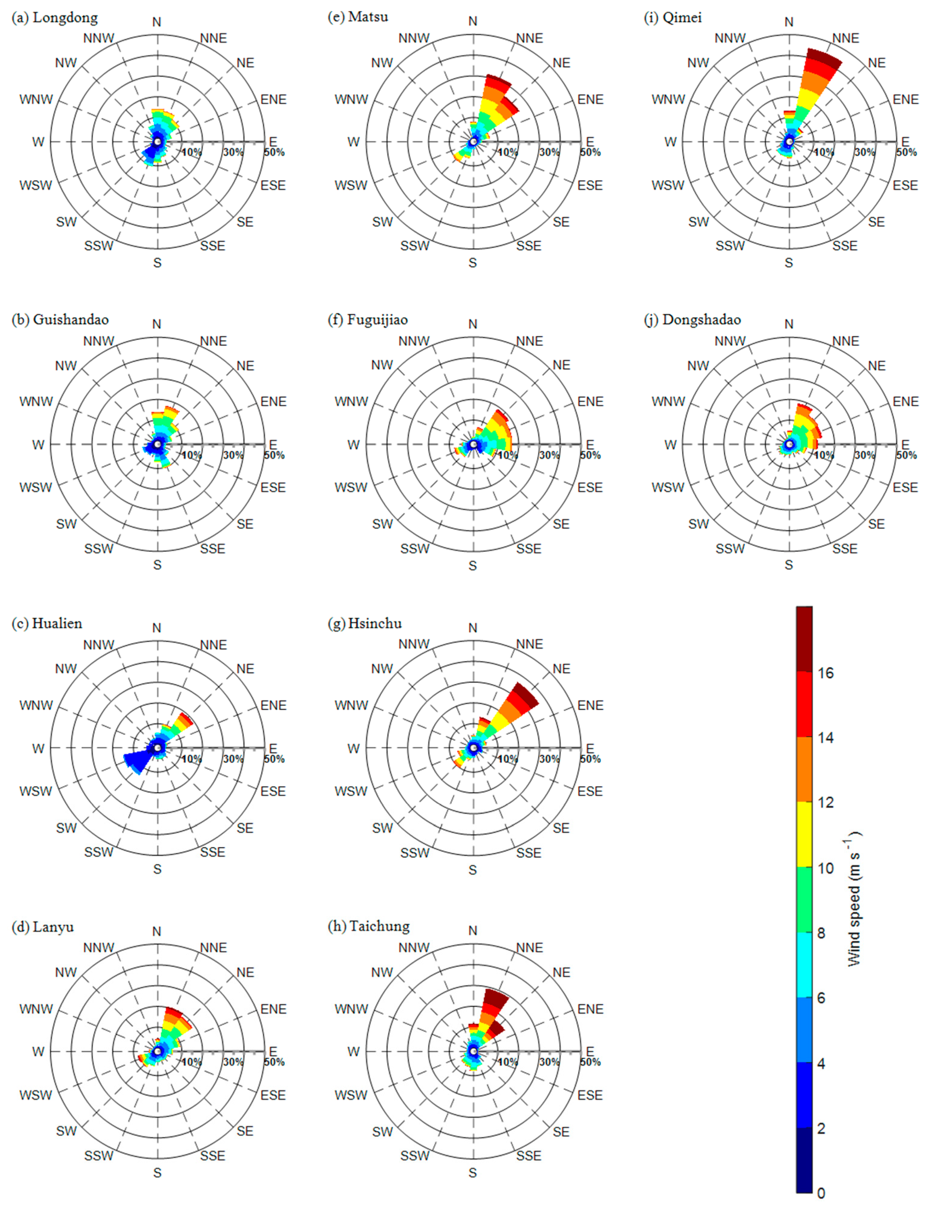
3.1. Wind Distribution

The distribution of wind direction and speed at a specific location over a defined temporal period can be effectively visualized using a wind rose diagram. Figure 2 presents the wind rose charts for the ten weather buoys spanning 2020–2024. The results indicate that northeasterly winds dominate in frequency, followed by southwesterly winds. This pattern is attributed to Taiwan’s geographic position in the southeastern Eurasian continent, where pronounced monsoon influences prevail. The northeast monsoon dominates during winter, while the southwest monsoon prevails in summer. Notably, northeasterly winds exhibit stronger speeds compared to southwesterly winds.

A comparative analysis of wind rose diagrams reveals distinct regional variations: buoys east of Taiwan (Figure 2a–d) exhibit weaker northeast wind speeds compared to those west of Taiwan (Figure 2e–j). Specifically, the four buoys in the Taiwan Strait (Matsu, Hsinchu, Taichung, and Qimei) demonstrate a higher proportion of strong winds (≥16 m s⁻¹). This phenomenon is likely influenced by the funneling effect of the Taiwan Strait, which amplifies wind velocities through topographic channeling.

Table 2. Mean and standard deviation of wind speed (unit: m s⁻¹).

Location	All	Spring	Summer	Autumn	Winter
Longdong	5.30 ± 2.86	4.76 ± 2.45	4.37 ± 2.74	5.54 ± 2.92	6.47 ± 2.86
Guishandao	5.70 ± 3.26	5.15 ± 2.94	4.54 ± 2.99	6.01 ± 3.26	6.99 ± 3.31
Hualien	4.49 ± 3.17	4.23 ± 2.81	3.33 ± 1.74	4.82 ± 3.40	5.54 ± 3.85
Lanyu	7.53 ± 3.75	7.00 ± 3.14	6.14 ± 3.53	8.07 ± 3.93	9.40 ± 3.48
Matsu	8.82 ± 3.88	7.35 ± 3.30	7.17 ± 3.20	9.97 ± 4.04	10.59 ± 3.61
Fuguijiao	7.50 ± 3.71	6.54 ± 3.27	5.66 ± 3.55	8.68 ± 3.53	8.83 ± 3.42
Hsinchu	8.42 ± 4.61	7.50 ± 4.02	6.82 ± 3.63	9.24 ± 5.14	9.95 ± 4.63
Taichung	9.09 ± 5.30	8.38 ± 4.64	5.92 ± 2.83	9.94 ± 5.78	13.03 ± 4.89
Qimei	8.30 ± 4.53	7.00 ± 3.76	5.20 ± 2.67	9.49 ± 4.77	11.38 ± 3.91
Dongshadao	8.39 ± 3.56	7.23 ± 3.14	6.23 ± 3.29	9.01 ± 3.53	10.52 ± 2.65

summarizes the mean and standard deviations of wind speeds across the ten buoys. The average wind speeds in eastern waters range from 4.49 m s⁻¹ to 7.53 m s⁻¹, while western waters exhibit higher velocities (7.50–9.09 m s⁻¹). Seasonal analysis reveals pronounced winter dominance, with eastern waters averaging 5.54–9.40 m s⁻¹ and western waters reaching 8.83–13.03 m s⁻¹, approximately 1.5 and 1.8 times the summer averages, respectively. Notably, Taichung and Qimei weather buoys exhibit winter wind speeds nearly double their summer counterparts.

The Taichung weather buoy consistently records the highest mean wind speed (9.09 m s⁻¹) and largest standard deviation (5.30 m s⁻¹), indicating the most pronounced variability in wind conditions. These findings underscore the critical role of geographic and seasonal factors in shaping wind patterns across Taiwan’s maritime regions.

3.2. Significant Wave Height

Figure 3 illustrates the rose diagrams of SWH measured at the ten weather buoys. The predominant wave direction at most buoys is from the northeast, with notable exceptions: the Hsinchu buoy primarily receives waves from the north, while the Lanyu weather buoy predominantly registers waves from the east. A comparison with the wind rose diagrams (Figure 2) reveals significant discrepancies between wind and wave directions at most buoys. For instance, at the Hsinchu weather buoy, winds are predominantly northeasterly, whereas waves originate from the north, resulting in a 45-degree directional difference. Similarly, at the Taichung weather buoy, winds are primarily from the north-northeast, yet waves predominantly propagate from the north. Conversely, certain buoys, such as the Qimei weather buoy, exhibit consistent wind and wave directions, both predominantly from the north-northeast.

The observed inconsistencies between wind and wave directions can be attributed to factors such as swell and buoy location. Buoys situated farther offshore, such as Qimei and Dongshadao weather buoys (as shown in Table 1), display more consistent wind–wave directional distributions. In contrast, buoys closer to shore, such as the Hualien weather buoy (located only 0.4 km from the coast), exhibit notable discrepancies. For example, while southwest winds are prominent in the wind rose diagram of the Hualien weather buoy, its SWH rose diagram shows no waves originating from the southwest. This discrepancy may result from Taiwan Island’s shielding effect to the southwest of the Hualien weather buoy, which mitigates the influence of weak southwest winds on wave generation. Similar conditions are observed at other eastern weather buoys (Longdong, Guishandao, and Lanyu), where landmass shielding reduces wave generation from southwest winds.

Table 3. Mean and standard deviation of SWH (unit: m).

Location	All	Spring	Summer	Autumn	Winter
Longdong	1.25 ± 0.84	1.11 ± 0.62	0.64 ± 0.63	1.47 ± 0.82	1.71 ± 0.83
Guishandao	0.99 ± 0.55	0.88 ± 0.40	0.73 ± 0.53	1.08 ± 0.61	1.24 ± 0.50
Hualien	1.10 ± 0.73	1.00 ± 0.56	0.58 ± 0.44	1.25 ± 0.72	1.54 ± 0.76
Lanyu	1.44 ± 0.92	1.25 ± 0.68	0.78 ± 0.56	1.75 ± 0.94	2.17 ± 0.79
Matsu	1.67 ± 0.93	1.35 ± 0.64	1.21 ± 0.74	1.99 ± 1.01	2.09 ± 0.93
Fuguijiao	1.36 ± 0.98	1.14 ± 0.72	0.64 ± 0.47	1.64 ± 1.02	1.96 ± 1.01
Hsinchu	1.09 ± 0.68	0.91 ± 0.50	0.60 ± 0.34	1.33 ± 0.74	1.47 ± 0.65
Taichung	1.42 ± 1.04	1.23 ± 0.82	0.59 ± 0.40	1.83 ± 1.07	2.22 ± 0.88
Qimei	1.33 ± 0.87	1.01 ± 0.63	0.90 ± 0.67	1.61 ± 0.99	1.75 ± 0.80
Dongshadao	1.97 ± 1.13	1.51 ± 0.84	1.30 ± 0.90	2.29 ± 1.20	2.61 ± 0.97

provides statistical summaries of SWH measured at the ten weather buoys. The average SWH ranges from 0.99 m to 1.44 m in eastern waters and from 1.09 m to 1.97 m in western waters. Seasonally, SWH is highest in winter, followed by autumn, with summer recording the lowest values, consistent with seasonal variations in wind speed. Winter averages range from 1.24 m to 2.17 m in eastern waters and from 1.47 m to 2.61 m in western waters.

Notably, there is no direct correlation between average SWH and average wind speed across all buoys. For instance, while the Dongshadao weather buoy records the highest average SWH despite not having the strongest average wind speed, the Taichung weather buoy, despite registering the highest average wind speed, ranks second in terms of average SWH. This disparity may be influenced by local sea conditions surrounding each weather buoy. The location of the Dongshadao weather buoy in open sea conditions within the northern South China Sea approximately 224 km offshore facilitates wave growth even under moderate wind speeds.

3.3. Wind–Wave Relationship

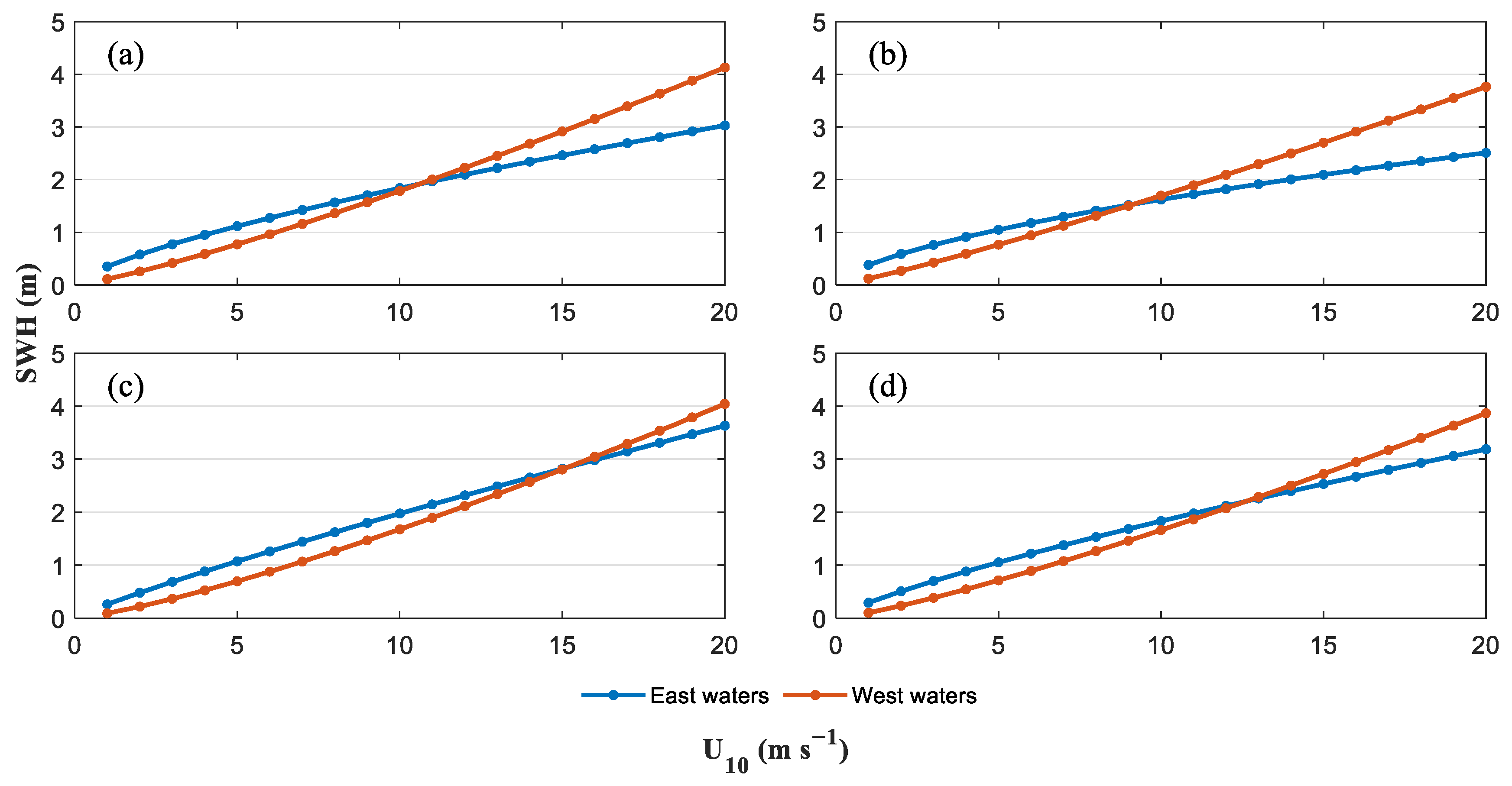
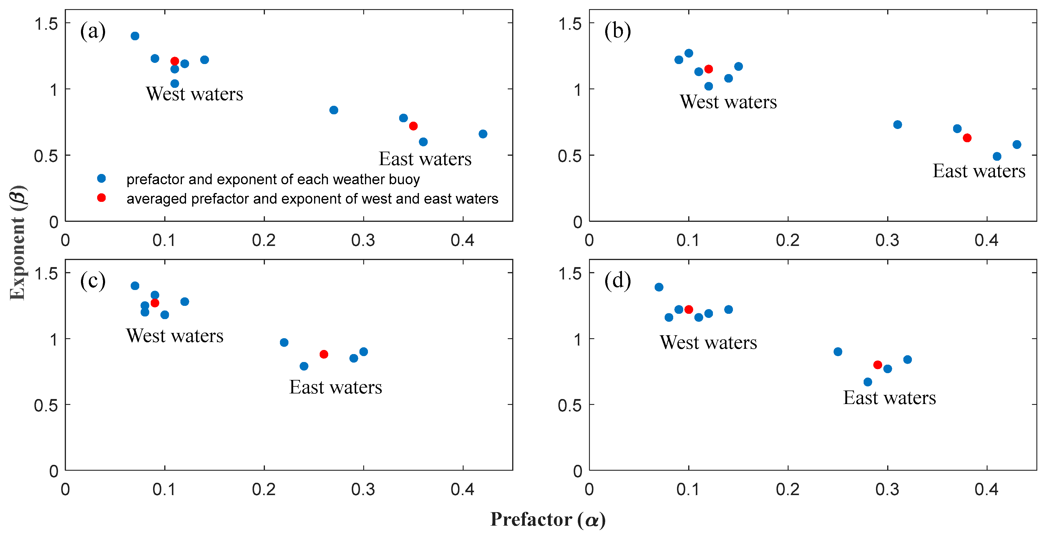
3.3.1. Regression Results

Table 4. α and β in Equation (4) derived from the best-fitting curve of the wind–wave relationship from the data collected between 2020 and 2024.

	All		T < 10 s		dir_diff < 45°		T < 10 s and dir_diff < 45°
Location	α	β	α	β	α	β	α	β
Longdong	0.34	0.78	0.37	0.70	0.30	0.90	0.32	0.84
Guishandao	0.36	0.60	0.41	0.49	0.24	0.79	0.28	0.67
Hualien	0.42	0.66	0.43	0.58	0.29	0.85	0.30	0.77
Lanyu	0.27	0.84	0.31	0.73	0.22	0.97	0.25	0.90
Matsu	0.07	1.40	0.10	1.27	0.07	1.40	0.07	1.39
Fuguijiao	0.12	1.19	0.14	1.08	0.09	1.33	0.12	1.19
Hsinchu	0.11	1.04	0.12	1.02	0.08	1.20	0.08	1.16
Taichung	0.09	1.23	0.09	1.22	0.10	1.18	0.11	1.16
Qimei	0.11	1.15	0.11	1.13	0.08	1.25	0.09	1.22
Dongshadao	0.14	1.22	0.15	1.17	0.12	1.28	0.14	1.22
East waters mean	0.35	0.72	0.38	0.63	0.26	0.88	0.29	0.80
West waters mean	0.11	1.21	0.12	1.15	0.09	1.27	0.10	1.22

presents the parameters α and β derived from regressing the best-fit curve of the relationship between $U_{10}$ and SWH at the ten weather buoys using the least squares method for the period spanning 2020–2024. To isolate wind waves from swells, criteria based on wave period (T) and direction alignment were applied: (1) T < 10 s and (2) wind and wave direction difference (dir_diff) < 45°. These thresholds minimized interference from swells while preserving wind-driven wave dynamics. The coefficient of determination (R²) and root mean square error (RMSE) of the regression results for all buoys are summarized in

Table 5. R² and RMSE (unit: m) of regression results.

	All		T < 10 s		dir_diff < 45°		T < 10 s and dir_diff < 45°
Location	R2	RMSE	R2	RMSE	R2	RMSE	R2	RMSE
Longdong	0.35	0.67	0.31	0.60	0.50	0.63	0.47	0.51
Guishandao	0.35	0.44	0.33	0.35	0.44	0.42	0.40	0.37
Hualien	0.37	0.58	0.32	0.46	0.57	0.57	0.56	0.46
Lanyu	0.36	0.73	0.34	0.62	0.66	0.53	0.66	0.44
Matsu	0.67	0.54	0.72	0.48	0.73	0.49	0.73	0.47
Fuguijiao	0.50	0.69	0.48	0.63	0.51	0.74	0.47	0.68
Hsinchu	0.62	0.42	0.61	0.41	0.65	0.41	0.64	0.40
Taichung	0.79	0.48	0.78	0.47	0.80	0.47	0.79	0.46
Qimei	0.70	0.48	0.72	0.43	0.74	0.45	0.75	0.42
Dongshadao	0.68	0.64	0.66	0.58	0.65	0.64	0.64	0.60
East waters mean	0.36	0.61	0.33	0.51	0.54	0.54	0.52	0.45
West waters mean	0.66	0.54	0.66	0.50	0.68	0.53	0.67	0.51

. While R² values vary across buoys, all regression results yield statistically significant p-values (<0.01), confirming the robustness of the wind–wave relationships. Notably, R² values in western waters (Figure 1) are consistently higher than those in eastern waters. Furthermore, distinguishing swells through the aforementioned criteria enhances R² values, particularly in eastern waters. Conversely, RMSE values exhibit no significant regional or methodological differences, suggesting comparable predictive accuracy across all cases.

The regression results reveal that all scaling exponents are substantially lower than the theoretical value of two, irrespective of whether all data or wind–wave-filtered data are utilized. This discrepancy suggests that the measurement locations may not correspond to fully developed sea conditions. Figure 4 illustrates the distribution of α and β across the ten weather buoys, revealing two distinct groupings that persist regardless of data filtering criteria. One group exhibits elevated α values paired with reduced β, while the other demonstrates lower α and higher β. Spatial analysis (Figure 1) indicates that these groupings correlate with geographic location: buoys in the eastern waters of Taiwan form the first cluster, while those in the western waters comprise the second.

To quantify these regional differences, the α and β values for the four eastern and six western buoys were averaged (Table 4). Substituting these mean parameters into the wind–wave relationship curves (Figure 5) yields contrasting dynamics. Figure 5 illustrates the differences in the wind–wave relationship between the eastern and western waters of Taiwan. Specifically, it shows how the SWH varies with $U_{10}$ under four different data filtering conditions (Figure 5a–d). In each subplot of Figure 5, a distinct intersection point is observed between the wind–wave relationship curves representing the eastern waters (blue line) and the western waters (orange line). This intersection point is critical. The wind speed corresponding to this point is approximately 12 m s⁻¹, slight variations may exist under different data filtering conditions, representing a crucial threshold. When the wind speed crosses this threshold, a shift occurs in the relative dominance of wave generation response between the eastern and western waters of Taiwan. Specifically, the significance of this intersection point can be elaborated as follows:

• When the wind speed is below the critical wind speed at the intersection point, the wind–wave relationship curve for the eastern waters lies above that of the western waters. This indicates that under relatively low wind speed conditions, the eastern waters generate a higher SWH for the same wind speed than the western waters. This phenomenon suggests that wave generation in the east of waters is more sensitive to wind in low-wind scenarios or that wave growth efficiency is higher.
• Conversely, the trend reverses when the wind speed exceeds the critical threshold. The wind–wave relationship curve for the western waters rises above that of the eastern waters. This means that the western waters produce a greater SWH under higher wind speed conditions than the eastern waters for the same wind speed. This may reflect specific geographical or oceanographic conditions in the western waters, such as fetch, bathymetry, or unique mechanisms of wind–wave interaction, all of which facilitate enhanced wave development at high wind speeds.

Figure 5. Curves of the wind-to-wave relationship using the average value in the waters east and west of Taiwan using (a) all data, (b) data with wave period less than 10 s, (c) data with direction difference less than 45°, and (d) data with wave period less than 10 s and direction difference less than 45°.

Figure 5. Curves of the wind-to-wave relationship using the average value in the waters east and west of Taiwan using (a) all data, (b) data with wave period less than 10 s, (c) data with direction difference less than 45°, and (d) data with wave period less than 10 s and direction difference less than 45°.

Therefore, this intersection point in Figure 5 marks a significant transition in wind speed. On either side of this point, the eastern and western waters of Taiwan demonstrate distinctly different wave development characteristics. This transition highlights that the wind–wave relationship exhibits non-linear characteristics and notable regional differences, significantly influenced by local geographical and oceanographic factors. These factors include variations in fetch length, bathymetric effect, and specific mechanisms of wind energy transfer to waves, all of which differ between the eastern and western waters of Taiwan.

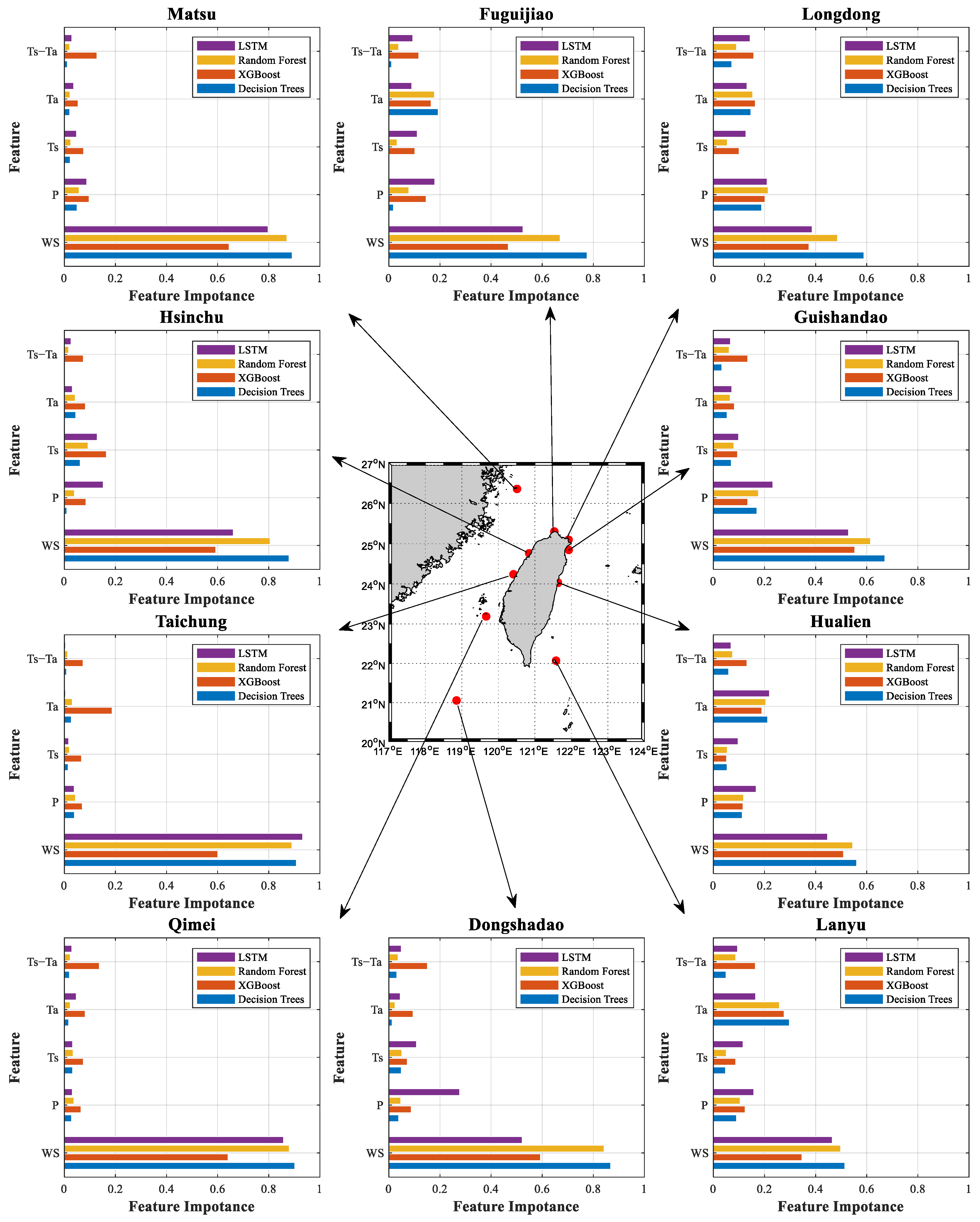
3.3.2. Regression Machine Learning Algorithms

Wave height prediction using machine learning methodologies necessitates prior model training. This study employed wind and wave data collected between 2020 and 2024 from ten weather buoys to train models, utilizing DT, XGBT, RF, and LSTM networks to evaluate algorithmic suitability for Taiwan’s marine environment.

DT algorithm quantifies feature weights through analysis of their contribution to decision-making processes. During training, decision trees partition nodes based on variance reduction, enhancing target variable homogeneity. Feature importance is computed as the aggregated contribution to impurity reduction across all splits where the feature is employed, with normalized scores providing relative weights. XGBT evaluates feature importance by measuring each feature’s contribution to reducing prediction errors during iterative training. It assigns weights to features by tracking their role in improving the model’s performance through gradient descent optimization. Common metrics for feature importance in XGBT include gain (improvement in accuracy from splits involving a feature), coverage (frequency of feature usage), and weight (number of times a feature is used for splitting). These metrics collectively provide insights into which features are most influential in the model. RF assesses feature importance using an ensemble-based approach. The algorithm aggregates multiple decision trees, and feature importance is calculated via the mean decrease in impurity method. For each tree, features that lead to greater reductions in impurity during node splits are assigned higher importance scores. These scores are then averaged across all trees in the forest and normalized to provide relative weights. This method ensures robust estimates of feature importance, even when individual trees may vary due to random sampling. LSTM networks are widely applied to time series forecasting due to their capacity to model temporal dependencies through gated recurrent architectures. While LSTMs excel at capturing long-term patterns, their performance can be optimized via hybrid architectures. However, interpreting LSTM weights remains challenging due to their interconnected nature, necessitating hybrid approaches, such as regularization or attention mechanisms, to indirectly assess feature importance. These methods enable the identification of dominant features while preserving LSTMs’ inherent strength in aggregating historical context. The training workflow for the four machine learning algorithms is illustrated in Figure 6.

Table 6. R² and RMSE (unit: m) of training results of four machine learning models.

Location	DT		XGBT		RF		LSTM
	R2	RMSE	R2	RMSE	R2	RMSE	R2	RMSE
Longdong	0.58	0.52	0.64	0.48	0.63	0.49	0.62	0.50
Guishandao	0.52	0.39	0.57	0.35	0.59	0.36	0.51	0.36
Hualien	0.58	0.44	0.62	0.40	0.61	0.40	0.61	0.40
Lanyu	0.65	0.53	0.75	0.45	0.72	0.48	0.70	0.49
Matsu	0.77	0.45	0.83	0.38	0.80	0.42	0.81	0.41
Fuguijiao	0.70	0.54	0.75	0.48	0.73	0.50	0.73	0.50
Hsinchu	0.76	0.33	0.82	0.28	0.79	0.31	0.79	0.31
Taichung	0.85	0.39	0.90	0.33	0.88	0.36	0.87	0.37
Qimei	0.76	0.42	0.81	0.38	0.79	0.39	0.79	0.39
Dongshadao	0.71	0.58	0.64	0.49	0.75	0.45	0.76	0.52
East waters mean	0.59	0.47	0.65	0.42	0.64	0.43	0.61	0.44
West waters mean	0.76	0.45	0.81	0.39	0.79	0.40	0.79	0.41

summarizes the training results of the four machine learning algorithms across the ten weather buoys. The performance metrics reveal that XGBT and RF demonstrate superior predictive accuracy, with minimal performance differences between them, followed by LSTM, while DT exhibits relatively weaker performance. All algorithms achieve R² values exceeding 0.5, with RMSE ranging from 0.25 m to 0.57 m.

Notably, the Taichung weather buoy yields the strongest performance across all algorithms, with R² values surpassing 0.85 and RMSE values below 0.39 m. Conversely, the Guishandao weather buoy consistently exhibits the poorest performance, with R² values ranging between 0.51 and 0.59, which are significantly lower than other buoys. However, RMSE values at the Guishandao weather buoy remain comparable to those of other buoys, suggesting that, while predictive accuracy is reduced, error magnitude remains consistent with regional variability.

Since wave fields are formed non-locally, AI models could potentially be improved by incorporating wind speed data from multiple weather buoys located at different sites. To explore this possibility, the data from weather buoys were grouped into western and eastern sections to determine if this division would enhance the results.

Table 7. R² and RMSE (unit: m) of training results of four machine learning models on eastern and western buoys.

Waters	DT		XGBT		RF		LSTM
	R2	RMSE	R2	RMSE	R2	RMSE	R2	RMSE
East	0.53	0.52	0.64	0.46	0.61	0.48	0.60	0.48
West	0.63	0.60	0.71	0.53	0.69	0.56	0.69	0.56

shows the R² and RMSE for AI models in the eastern and western waters of Taiwan. Compared with the results shown in Table 6, it seems that this approach of grouping to eastern and western waters does not improve the training results.

A comparative analysis of regression and machine learning methods reveals that the latter (XGBT, RF, LSTM, and DT) outperformed regression in both predictive accuracy and error metrics. Specifically, machine learning models achieved statistically significant improvements in R² and marginally reduced RMSE. Consistent with regression results, the Taichung weather buoy demonstrated the highest R² value across all methodologies, while waters west of Taiwan exhibited superior performance compared to eastern regions in both regression and AI-driven analyses.

The analysis results show regional disparities, with higher R² values in the western waters, and divergent α and β values between the waters east and west of Taiwan. These differences are discussed in the next section.

4. Discussion

The regression analysis reveals significant spatial heterogeneity in α and β of the wind–wave relationship between the waters east and west of Taiwan. Concurrently, weather buoys provide ancillary data on air pressure, air temperature, and sea surface temperature alongside wind speed and wave measurements. These variables, combined with sea-air temperature differences, were incorporated as feature variables to investigate their potential influence on wave growth.

To elucidate the regional disparities in wind–wave relationships, feature importance analyses were conducted for the four machine learning algorithms (DT, XGBT, RF, LSTM). Figure 7 presents the weights of feature variables across all buoys. While wind speed emerges as the dominant feature in all models and locations, its relative importance varies spatially. For the two highest-performing algorithms (XGBT and RF), wind speed weights in western waters (0.59–0.64 for XGBT, except the Fuguijiao weather buoy at 0.47; >0.81 for RF, except the Fuguijiao weather buoy at 0.67) exceed those in eastern waters (0.34–0.50 for XGBT; <0.61 for RF). This suggests that wind speed is the primary driver of wave growth in the waters west of Taiwan, with minimal influence from secondary factors. Conversely, eastern waters exhibit lower wind speed weights, with air pressure and air temperature contributing approximately 1/3 to 1/2 of the wind speed’s influence. The disparity in wind speed weights aligns with regional wind speed differences (Table 2), where western waters exhibit stronger winds. This may explain the superior regression performance in western Taiwan, as higher wind speeds enhance wind–wave coupling.

The prominence of air pressure and air temperature in eastern waters warrants further consideration. While no direct causal relationship exists between these variables and wave height, their influence may be mediated by meteorological phenomena. For instance, air pressure gradients drive wind generation, with low-pressure systems (e.g., typhoons) producing stronger winds that transfer kinetic energy to the ocean surface via shear forces [19]. Similarly, air temperature fluctuations, common at weather fronts, may indirectly affect wave dynamics through their association with wind patterns. Taiwan’s eastern waters are frequently impacted by weather fronts and typhoons, which introduce variability in air pressure and temperature. These factors likely contribute to the observed α and β divergence and algorithmic performance differences between the waters east and west of Taiwan.

The calculation of $U_{10}$ (as shown in Equation (8)) is based on the assumption of neutral atmospheric stratification. However, if the stratification is non-neutral, it can be influenced by factors such as air temperature, water temperature, and humidity [50]. This may help explain the analysis results from AI models, which show that the wind–wave relationship at some weather buoys is significantly affected by air and sea temperatures. This effect is particularly evident in the eastern waters of Taiwan, resulting in poor results for the wind–wave relationship.

Moreover, the differences between the waters east and west of Taiwan, as well as the reasons for the model’s poorer performance in the eastern waters, likely arise from fetch limitations and swell dominance. Weather buoys in the waters east of Taiwan face shorter fetches due to their proximity to land, which limits wave growth despite similar wind speeds. The waters east of Taiwan may experience more intense swells from open-ocean sources, complicating local wind–wave dynamics.

Although the empirical coefficients derived from this study do not seem to fully distinguish between wind waves and swells in terms of wave period and wind–wave alignment, this study still provides valuable insights. It is suggested that future data collection include more wave parameters, such as wave steepness, because wind waves typically exhibit sharp crests and a relatively large ratio of wave height to wavelength due to the continuous action and energy input of local winds.

5. Conclusions

This study provides a comprehensive analysis of wind–wave interactions around Taiwan, leveraging a unique dataset of wind and wave measurements from ten weather buoys collected between 2020 and 2024. By integrating traditional regression analyses with advanced machine learning techniques, the research elucidates the complex dynamics governing SWH.

Key findings reveal the dominance of northeasterly winds due to Taiwan’s geographic location and monsoon climate. A distinct regional variation in wind speeds and wave heights was observed between the eastern and western waters. The averaged wind speed measured by the buoys in the Taiwan Strait ranges from 8.30 to 9.09 m s⁻¹, which is stronger than that measured in the eastern waters of Taiwan, ranging from 4.49 to 7.53 m s⁻¹. Specifically, buoys in the Taiwan Strait showed a higher proportion of strong winds, likely due to the funneling effect. Additionally, the machine learning models demonstrated better analysis results compared to conventional regression methods, capturing complex, nonlinear relationships between wind speed and SWH. The R² value for the eastern waters improved from 0.33 to 0.54 with conventional regression methods to 0.59–0.65 using machine learning. In the western waters, it increased from 0.66–0.68 to 0.76–0.81. The RMSE in the eastern waters decreased from 0.45 to 0.61 m with conventional regression methods to 0.42–0.47 m using machine learning, while in the western waters, it dropped from 0.51–0.54 m to 0.39–0.45 m. These models offer a robust framework for understanding air–sea interactions and supporting maritime operations, coastal engineering, renewable energy development, and climate change adaptation efforts in the region. By bridging the gap between traditional analytical methods and AI approaches, this research contributes valuable insights for sustainable maritime practices and coastal resilience in Taiwan’s dynamic marine environment.

References

1. Cimarelli, A.; Romoli, F.; Stalio, E. On wind–wave interaction phenomena at low Reynolds numbers. J. Fluid Mech. 2023, 956, A13. [Google Scholar] [CrossRef]
2. Hou, B.; Fu, H.; Li, X.; Song, T.; Zhang, Z. Predicting significant wave height in the South China Sea using the SAC-ConvLSTM model. Front. Mar. Sci. 2024, 11, 1424714. [Google Scholar] [CrossRef]
3. Zhan, Y.; Zhang, H.; Li, J.; Li, G. Prediction method for ocean wave height based on stacking ensemble learning model. J. Mar. Sci. Eng. 2022, 10, 1150. [Google Scholar] [CrossRef]
4. Bujak, D.; Bogovac, T.; Carević, D.; Miličević, H. Filling Missing and Extending Significant Wave Height Measurements Using Neural Networks and an Integrated Surface Database. Wind 2023, 3, 151–169. [Google Scholar] [CrossRef]
5. Carrasco, R.; Horstmann, J.; Seemann, J. Significant wave height measured by coherent X-band radar. IEEE Trans. Geosci. Remote Sens. 2017, 55, 5355–5365. [Google Scholar] [CrossRef]
6. Woo, H.J.; Park, K.A. Estimation of extreme significant wave height in the northwest pacific using satellite altimeter data focused on typhoons (1992–2016). Remote Sens. 2021, 13, 1063. [Google Scholar] [CrossRef]
7. Ouyang, L.; Ling, F.; Li, Y.; Bai, L.; Luo, J.J. Wave forecast in the Atlantic Ocean using a double-stage ConvLSTM network. Atmos. Ocean. Sci. Lett. 2023, 16, 100347. [Google Scholar] [CrossRef]
8. Song, T.; Han, R.; Meng, F.; Wang, J.; Wei, W.; Peng, S. A significant wave height prediction method based on deep learning combining the correlation between wind and wind waves. Front. Mar. Sci. 2022, 9, 983007. [Google Scholar] [CrossRef]
9. Medina-Manuel, A.; Molina Sánchez, R.; Souto-Iglesias, A. AI-Driven Model Prediction of Motions and Mooring Loads of a Spar Floating Wind Turbine in Waves and Wind. J. Mar. Sci. Eng. 2024, 12, 1464. [Google Scholar] [CrossRef]
10. Wang, X.; Jiang, H. Physics-guided deep learning for skillful wind-wave modeling. Sci. Adv. 2024, 10, eadr3559. [Google Scholar] [CrossRef]
11. Shen, J.; Zhang, J.; Qiu, Y.; Li, L.; Zhang, S.; Pan, A.; Huang, J.; Guo, X.; Jing, C. Winter counter-wind current in western Taiwan Strait: Characteristics and mechanisms. Cont. Shelf Res. 2019, 172, 1–11. [Google Scholar] [CrossRef]
12. Cheng, K.S.; Ho, C.Y.; Teng, J.H. Wind characteristics in the Taiwan strait: A case study of the first offshore wind farm in Taiwan. Energies 2020, 13, 6492. [Google Scholar] [CrossRef]
13. Dong, S.; Gong, Y.; Wang, Z. Long-term variations of wind and wave conditions in the Taiwan Strait. Reg. Stud. Mar. Sci. 2020, 36, 101256. [Google Scholar] [CrossRef]
14. Lu, W.S.; Tseng, C.H.; Hsiao, S.C.; Chiang, W.S.; Hu, K.C. Future Projection for Wave Climate around Taiwan Using Weather-Type Statistical Downscaling Method. J. Mar. Sci. Eng. 2022, 10, 1823. [Google Scholar] [CrossRef]
15. Doong, D.J.; Fan, Y.M.; Chen, J.Y.; Kao, C.C. Analysis of Long-Period Hazardous Waves in the Taiwan Marine Environment Monitoring Service. Front. Mar. Sci. 2021, 8, 657569. [Google Scholar] [CrossRef]
16. Doong, D.J.; Tsai, C.H.; Chen, Y.C.; Peng, J.P.; Huang, C.J. Statistical analysis on the long-term observations of typhoon waves in the Taiwan sea. J. Mar. Sci. Tech. 2015, 23, 893–900. [Google Scholar] [CrossRef]
17. Ou, Y.; Zhai, F.; Li, P. Interannual wave climate variability in the Taiwan Strait and its relationship to ENSO events. J. Oceanol. Limnol. 2018, 36, 2110–2129. [Google Scholar] [CrossRef]
18. Chien, H.; Cheng, H.Y.; Chiou, M.D. Wave climate variability of Taiwan waters. J. Oceanogr. 2014, 70, 133–152. [Google Scholar] [CrossRef]
19. Doong, D.J.; Chen, S.H.; Kao, C.C.; Lee, B.C.; Yeh, S.P. Data quality check procedures of an operational coastal ocean monitoring network. Ocean Eng. 2007, 34, 234–246. [Google Scholar] [CrossRef]
20. Longuet-Higgins, M.S.; Cartwright, D.E.; Smith, N.D. Observations of the directional spectrum of sea waves using the motions of a floating buoy. In Ocean Wave Spectra; Prentice-Hall: Saddle River, NJ, USA, 1963; pp. 111–136. [Google Scholar]
21. Lygre, A.; Krogstad, H.E. Maximum entropy estimation of the directional distribution in ocean wave spectra. J. Phys. Oceanogr. 1986, 16, 2052–2060. [Google Scholar] [CrossRef]
22. Capon, J. Maximum-likelihood spectral estimation. In Nonlinear Methods in Spectral Analysis; Heykin, S., Ed.; Springer: New York, NY, USA, 1979; pp. 155–179. [Google Scholar] [CrossRef]
23. Hashimoto, N.; Kobune, K. Directional spectrum estimation from a Bayesian approach. In Proceedings of the American Society of Civil Engineers 21st International Conference on Coastal Engineering, Costa del SoL-MaLaga, Spain, 20–25 June 1988; pp. 62–76. [Google Scholar] [CrossRef]
24. Falnes, J. A review of wave-energy extraction. Mar. Struct. 2007, 20, 185–201. [Google Scholar] [CrossRef]
25. World Meteorological Organization. Guide to Wave Analysis and Forecasting, 2018th ed.; World Meteorological Organization: Geneva, Switzerland, 2018; pp. 1–189. [CrossRef]
26. Gao, Y.; Schmitt, F.G.; Hu, J.; Huang, Y. Probability-based wind-wave relation. Front. Mar. Sci. 2023, 9, 1085340. [Google Scholar] [CrossRef]
27. Lee, Y.C.; Doong, D.J. Duration-limited growth method for wind sea and swell separation of directional wave spectrum. Ocean Eng. 2025, 329, 121182. [Google Scholar] [CrossRef]
28. Kinsman, B. Wind Waves: Their Generation and Propagation on the Ocean Surface; Prentice-Hall, Inc.: Englewood Cliffs, NJ, USA, 1984; pp. 1–676. [Google Scholar]
29. Hanson, J.L.; Phillips, O.M. Wind sea growth and dissipation in the open ocean. J. Phys. Oceanogr. 1999, 29, 1633–1648. [Google Scholar] [CrossRef]
30. Vettor, R.; Soares, C.G. A global view on bimodal wave spectra and crossing seas from ERA-interim. Ocean Eng. 2020, 210, 107439. [Google Scholar] [CrossRef]
31. Wang, G.; Zhang, K.; Shi, J. The Effect of Different Swell and Wind-Sea Proportions on the Transformation of Bimodal Spectral Waves over Slopes. Water 2024, 16, 296. [Google Scholar] [CrossRef]
32. Snodgrass, F.E.; Hasselmann, K.F.; Miller, G.R.; Munk, W.H.; Powers, W.H. Propagation of ocean swell across the Pacific. Philos. Trans. A Math. Phys. Eng. Sci. 1966, 259, 431–497. [Google Scholar] [CrossRef]
33. Yan, Y.; Hu, M.; Ni, Y.; Qiu, C. Simulated Directional Wave Spectra of the Wind Sea and Swell under Typhoon Mangkhut. Atmosphere 2024, 15, 1174. [Google Scholar] [CrossRef]
34. Davis, J.R.; Thomson, J.; Houghton, I.A.; Fairall, C.W.; Butterworth, B.J.; Thompson, E.J.; de Boer, G.; Doyle, J.D.; Moskaitis, J.R. Ocean surface wave slopes and wind-wave alignment observed in Hurricane Idalia. J. Geophys. Res. Oceans 2025, 130, e2024JC021814. [Google Scholar] [CrossRef]
35. Wyatt, L.R.; Green, J.J. Swell and wind-sea partitioning of HF radar directional spectra. J. Oper. Oceanogr. 2024, 17, 28–39. [Google Scholar] [CrossRef]
36. Pierson Jr, W.J.; Moskowitz, L. A proposed spectral form for fully developed wind seas based on the similarity theory of SA Kitaigorodskii. J. Geophys. Res. 1964, 69, 5181–5190. [Google Scholar] [CrossRef]
37. Liu, P.L.F.; Losada, I.J. Wave propagation modeling in coastal engineering. J. Hydraul. Res. 2002, 40, 229–240. [Google Scholar] [CrossRef]
38. Ribal, A.; Young, I.R. 33 years of globally calibrated wave height and wind speed data based on altimeter observations. Sci. Data 2019, 6, 77. [Google Scholar] [CrossRef]
39. Guan, C.; Xie, L. On the linear parameterization of drag coefficient over sea surface. J. Phys. Oceanogr. 2004, 34, 2847–2851. [Google Scholar] [CrossRef]
40. Quinlan, J.R. Induction of decision trees. Mach. Learn. 1986, 1, 81–106. [Google Scholar] [CrossRef]
41. Patel, H.H.; Prajapati, P. Study and analysis of decision tree based classification algorithms. Int. J. Comput. Sci. Eng. 2018, 6, 74–78. [Google Scholar] [CrossRef]
42. Chen, T.; Guestrin, C. Xgboost: A scalable tree boosting system. In Proceedings of the 22nd ACM SIGKDD International Conference on Knowledge Discovery and Data Mining, San Francisco, CA, USA, 13–17 August 2016. [Google Scholar] [CrossRef]
43. Breiman, L. Random forests. Mach. Learn. 2001, 45, 5–32. [Google Scholar] [CrossRef]
44. Liaw, A.; Wiener, M. Classification and regression by randomForest. R News 2002, 2, 18–22. [Google Scholar]
45. Biau, G. Analysis of a random forests model. J. Mach. Learn. Res. 2012, 13, 1063–1095. [Google Scholar]
46. Hochreiter, S.; Schmidhuber, J. Long short-term memory. Neural Comput. 1997, 9, 1735–1780. [Google Scholar] [CrossRef]
47. Greff, K.; Srivastava, R.K.; Koutník, J.; Steunebrink, B.R.; Schmidhuber, J. LSTM: A search space odyssey. IEEE Trans. Neural Netw. Learn. Syst. 2015, 28, 2222–2232. [Google Scholar] [CrossRef] [PubMed]
48. Noh, S.-H. Analysis of gradient vanishing of RNNs and performance comparison. Information 2021, 12, 442. [Google Scholar] [CrossRef]
49. Sahoo, B.B.; Jha, R.; Singh, A.; Kumar, D. Long short-term memory (LSTM) recurrent neural network for low-flow hydrological time series forecasting. Acta Geophys. 2019, 67, 1471–1481. [Google Scholar] [CrossRef]
50. Fairall, C.W.; Bradley, E.F.; Hare, J.E.; Grachev, A.A.; Edson, J.B. Bulk parameterization of air–sea fluxes: Updates and verification for the COARE algorithm. J. Clim. 2003, 16, 571–591. [Google Scholar] [CrossRef]
Figure 1. Location of weather buoy in Taiwan waters. The black dashed line divides the waters into east waters and west waters. The weather buoys in the east waters include Longdon, Guishandao, Hualien, and Lanyu, while the west waters include Matsu, Fuguijiao, Hsinchu, Taichung, Qimei, and Dongshadao.
Jmse 13 01047 g001
Figure 2. Wind rose chart measured at the ten weather buoys. (ad) are located in the waters east of Taiwan, and (ej) are located in the waters west of Taiwan.
Jmse 13 01047 g002
Figure 3. Same as Figure 2, but for SWH.
Jmse 13 01047 g003
Figure 4. Distribution of α and β of the wind-to-wave relationship at the ten weather buoys. Two red dots represent the average of the prefactor and scaling exponent of weather buoys in the waters east (lower right) and west (upper left) of Taiwan, respectively, derived using (a) all data, (b) data with wave period less than 10 s, (c) data with direction difference less than 45°, and (d) data with wave period less than 10 s and direction difference less than 45°.
Jmse 13 01047 g004
Figure 6. Training flow chart of the four machine learning algorithms. (a) DT, (b) XGBT, (c) RF, and (d) LSTM.
Jmse 13 01047 g006
Figure 7. Feature weights for SWH of ten weather buoys using DT, XGBT, RF, and LSTM machine learning algorithms.
Jmse 13 01047 g007