
Optimal Alternative Fuel Selection for Dual-Fuel Ships Under FuelEU Maritime Regulations: Environmental and Economic Assessment

Abstract
1. Introduction
2. Method and Data
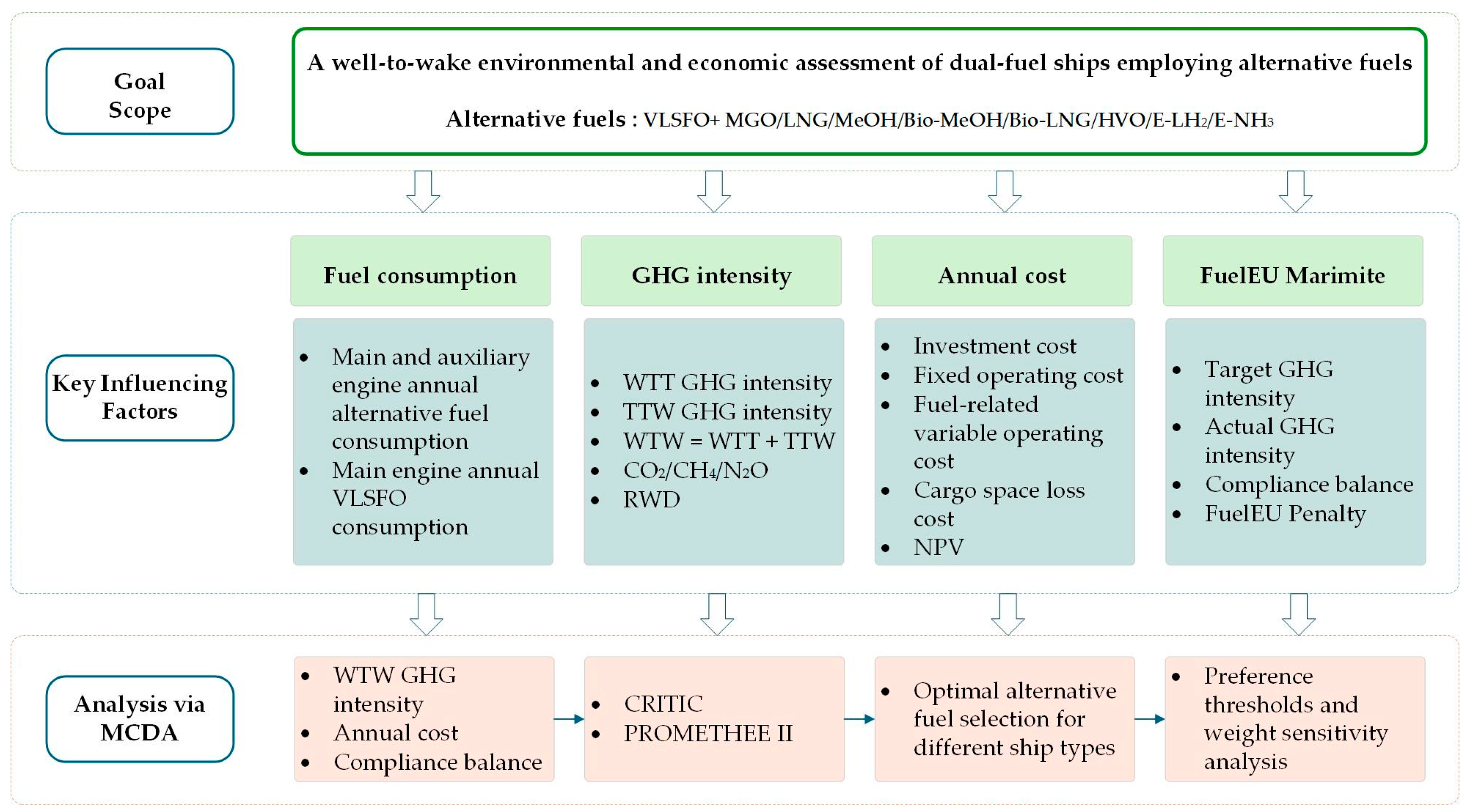
2.1. Method
2.1.1. Calculation of Fuel Consumption for Dual-Fuel Ships
2.1.2. Well-to-Wake GHG Intensity Calculation Model
2.1.3. Annual Cost Calculation Model
2.1.4. FuelEU Penalty Calculation Model
2.1.5. PROMETHEE II Method
2.2. Data
2.2.1. Case Study Ships
2.2.2. Fuel Data
3. Results
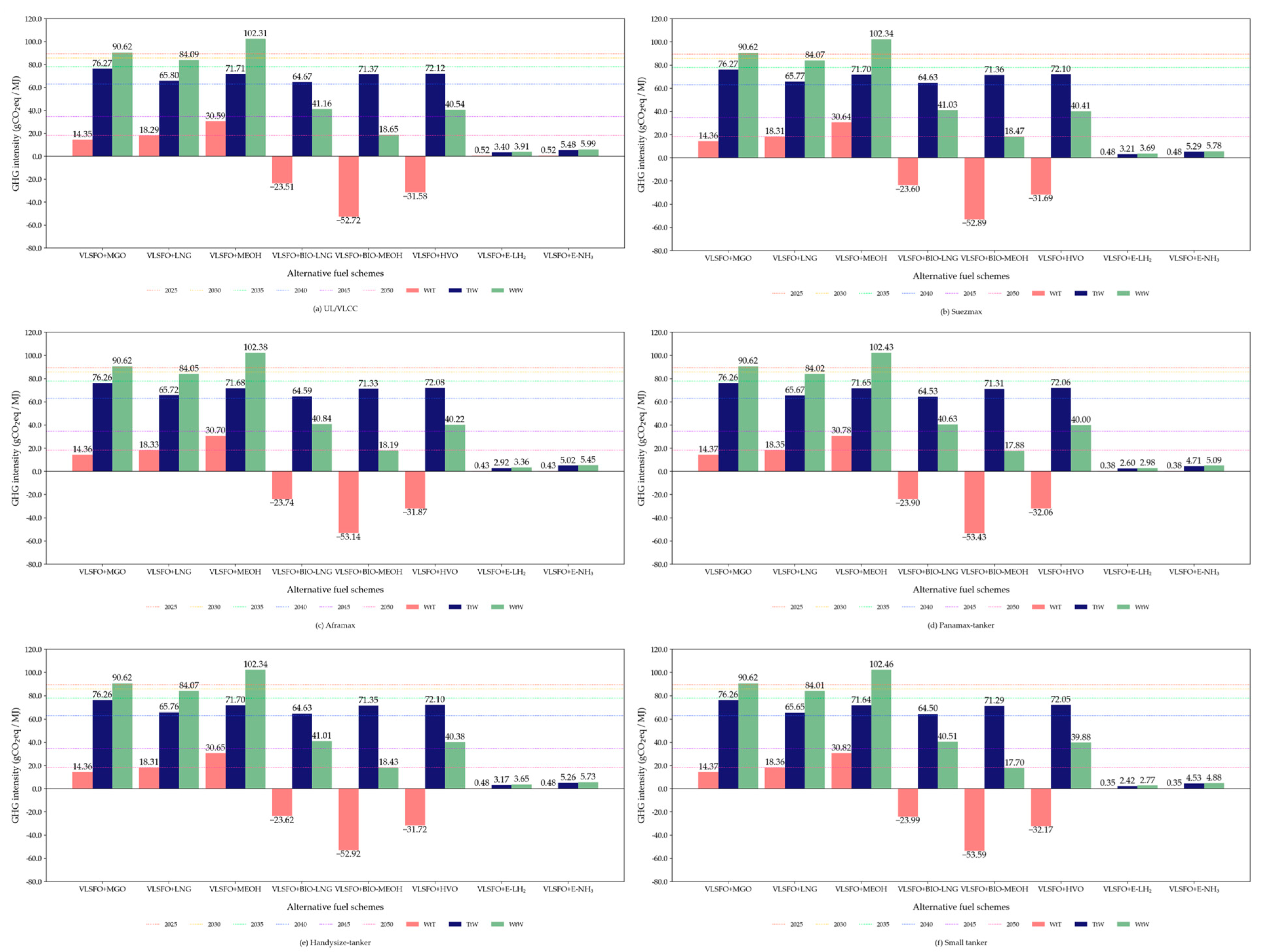
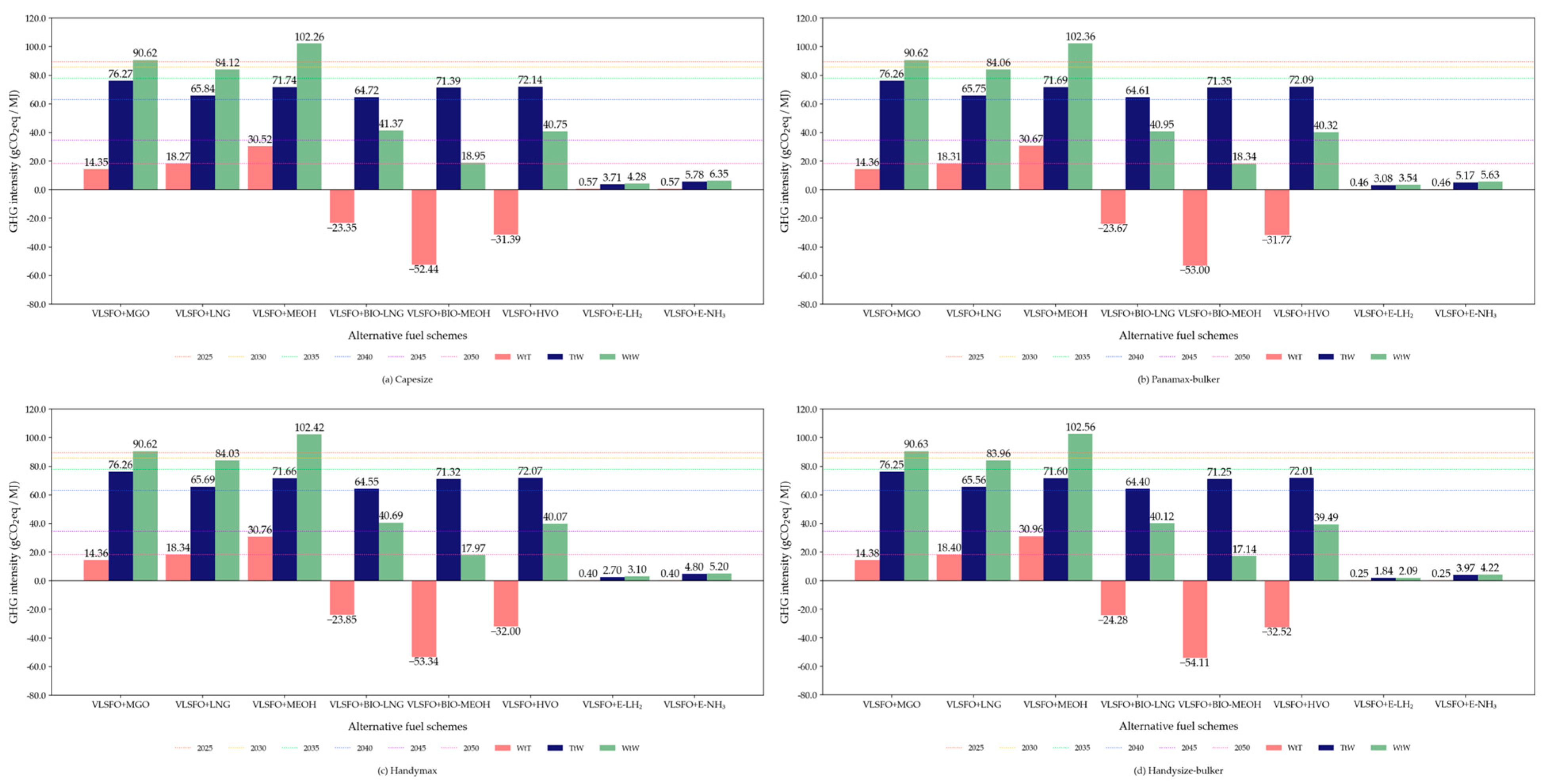
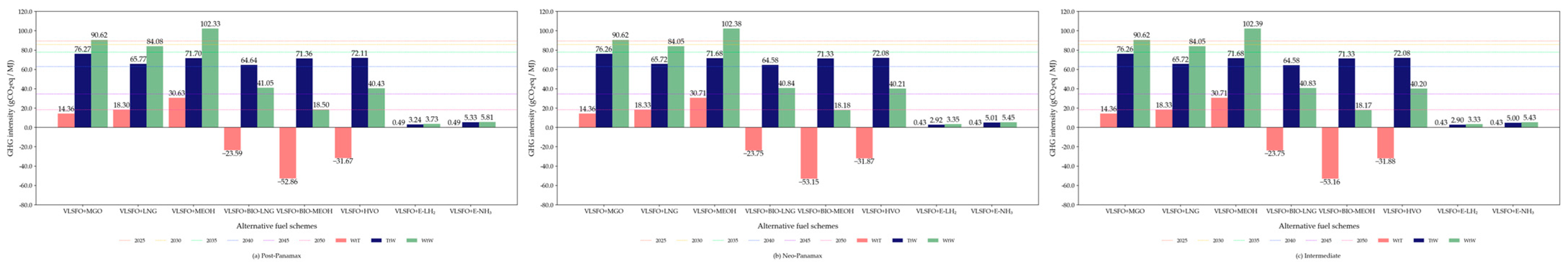
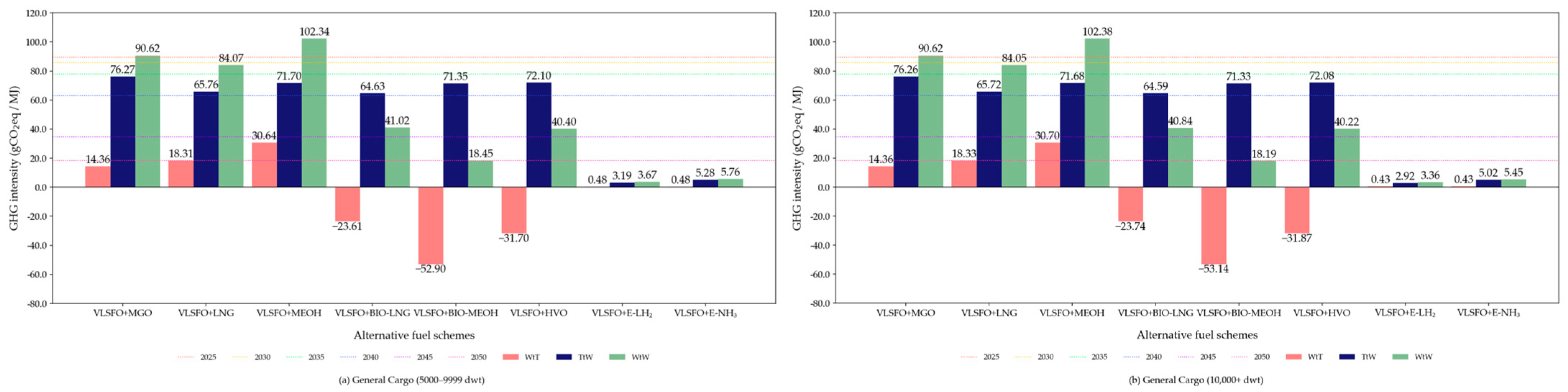
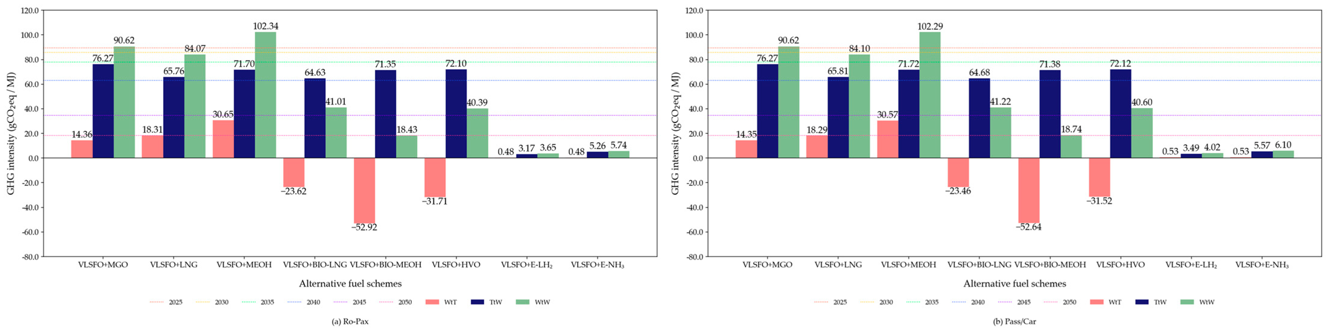
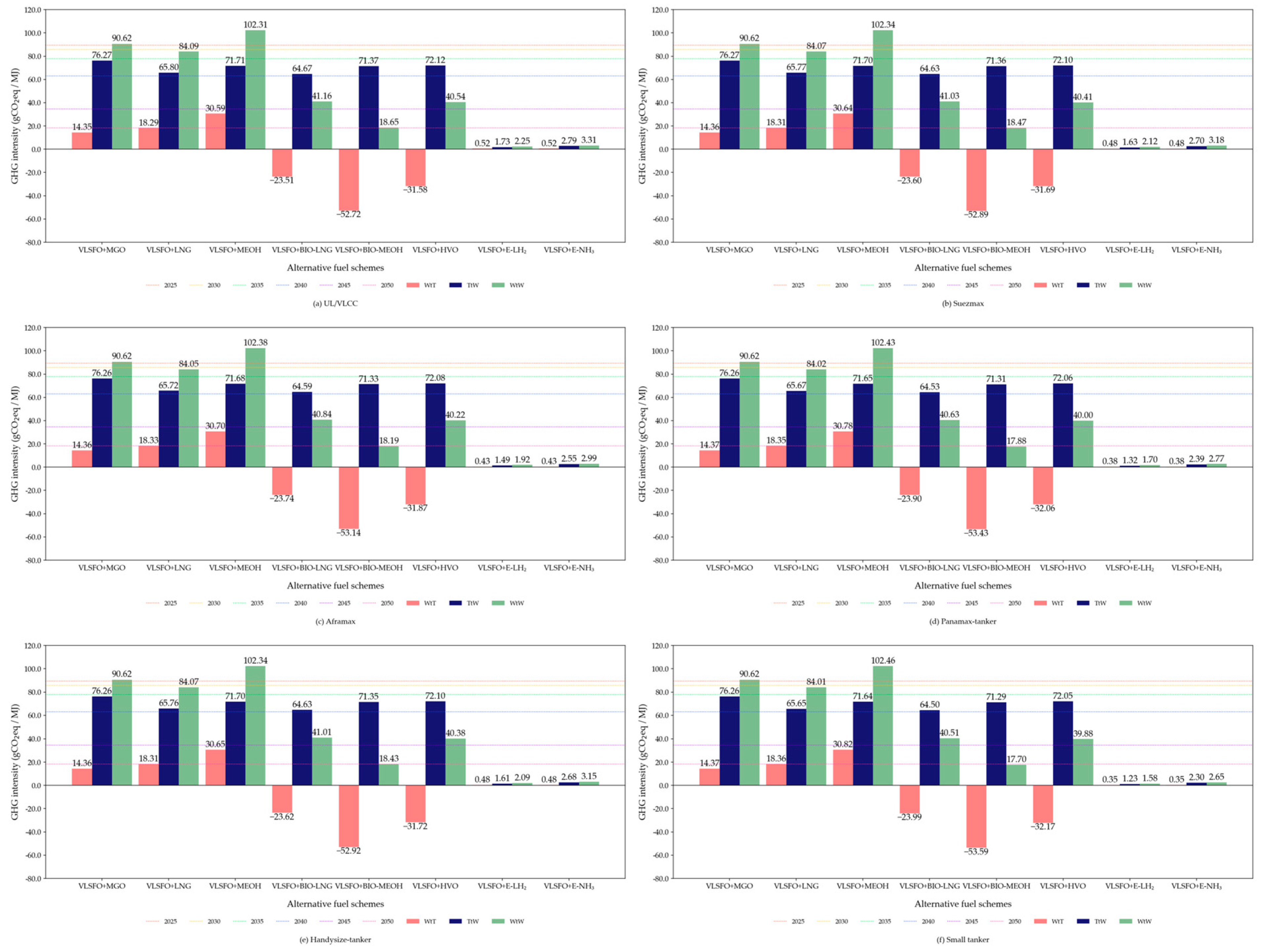
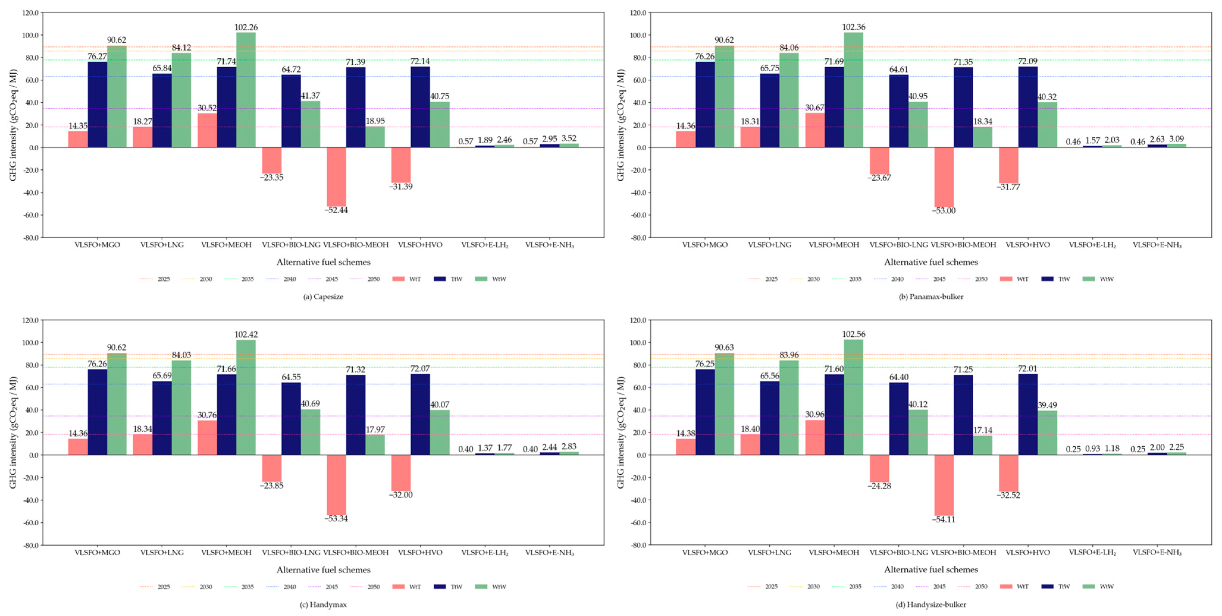
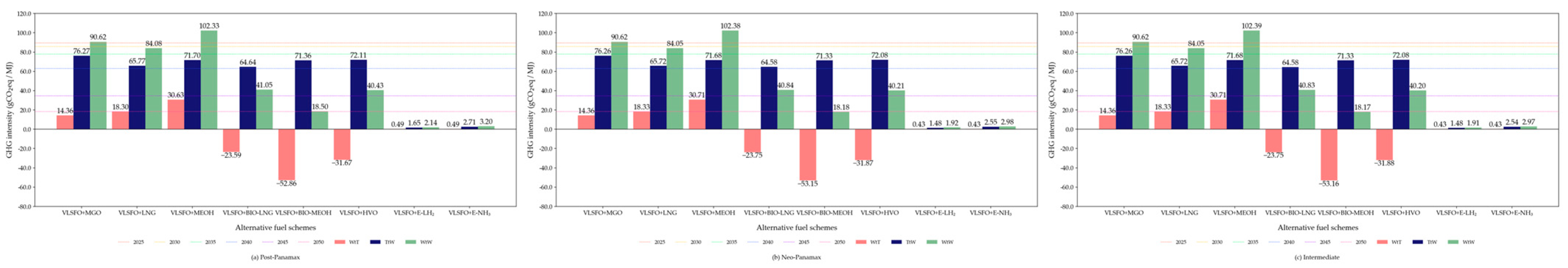
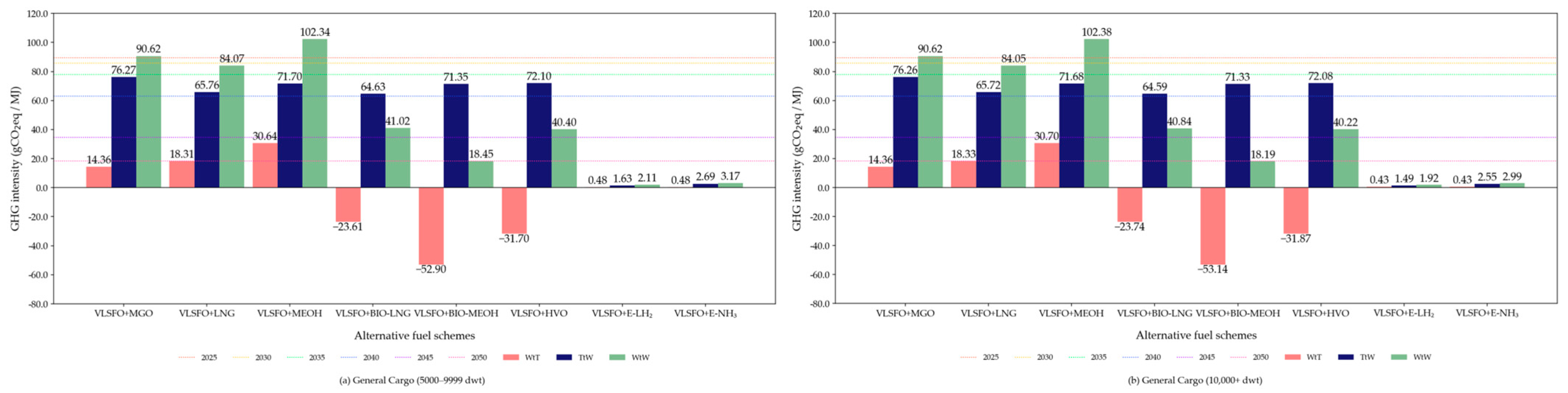
3.1. Environmental Assessment of Alternative Fuels
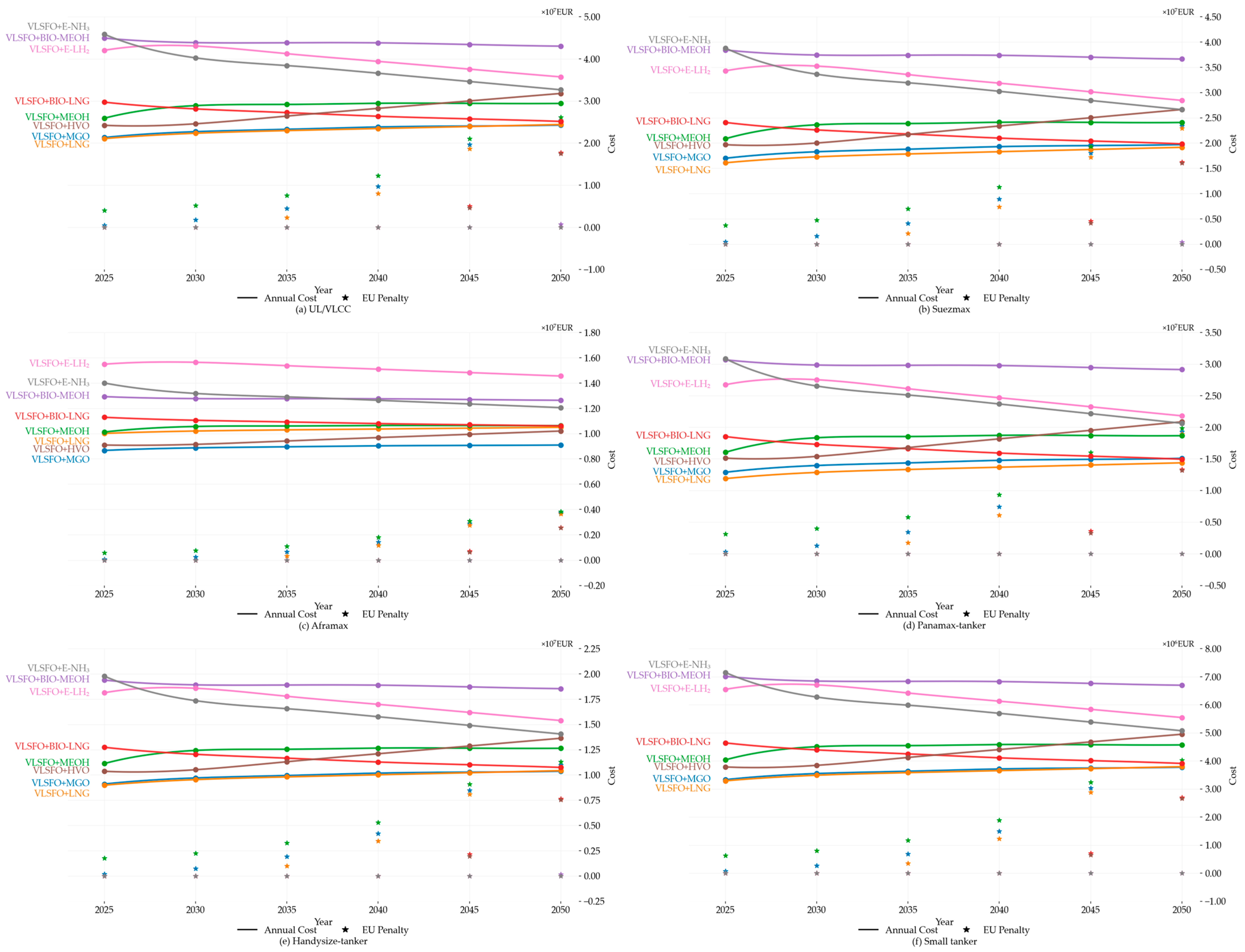
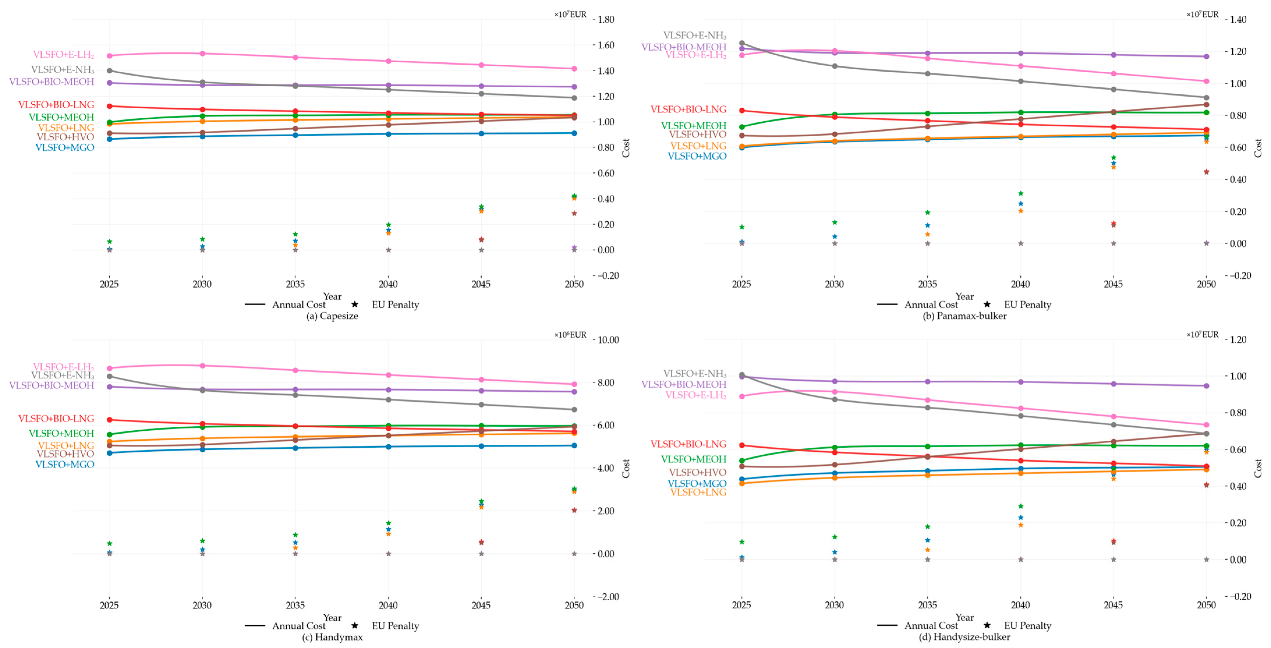
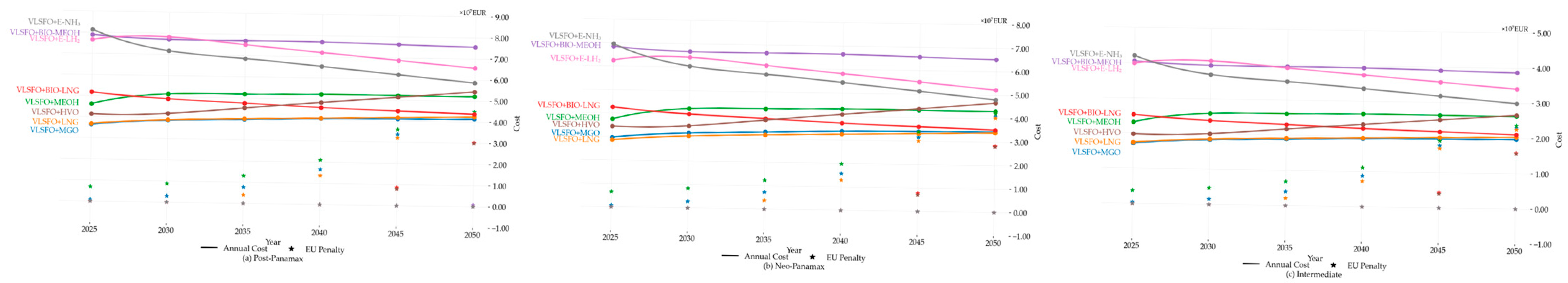
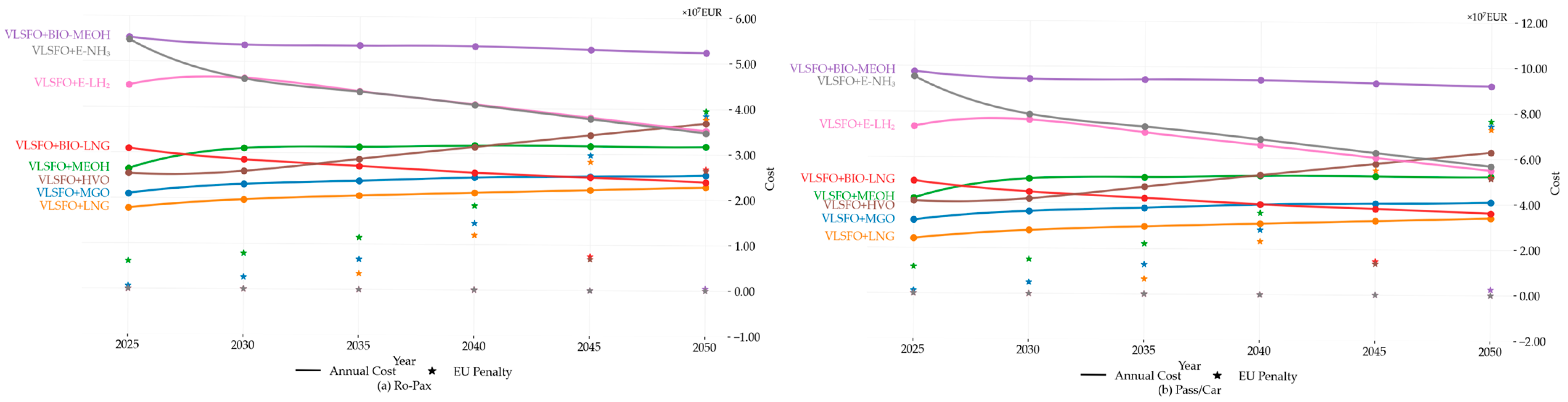
3.2. Economic and Compliance Assessment of Alternative Fuels
3.3. Optimal Selection of Alternative Fuel Options
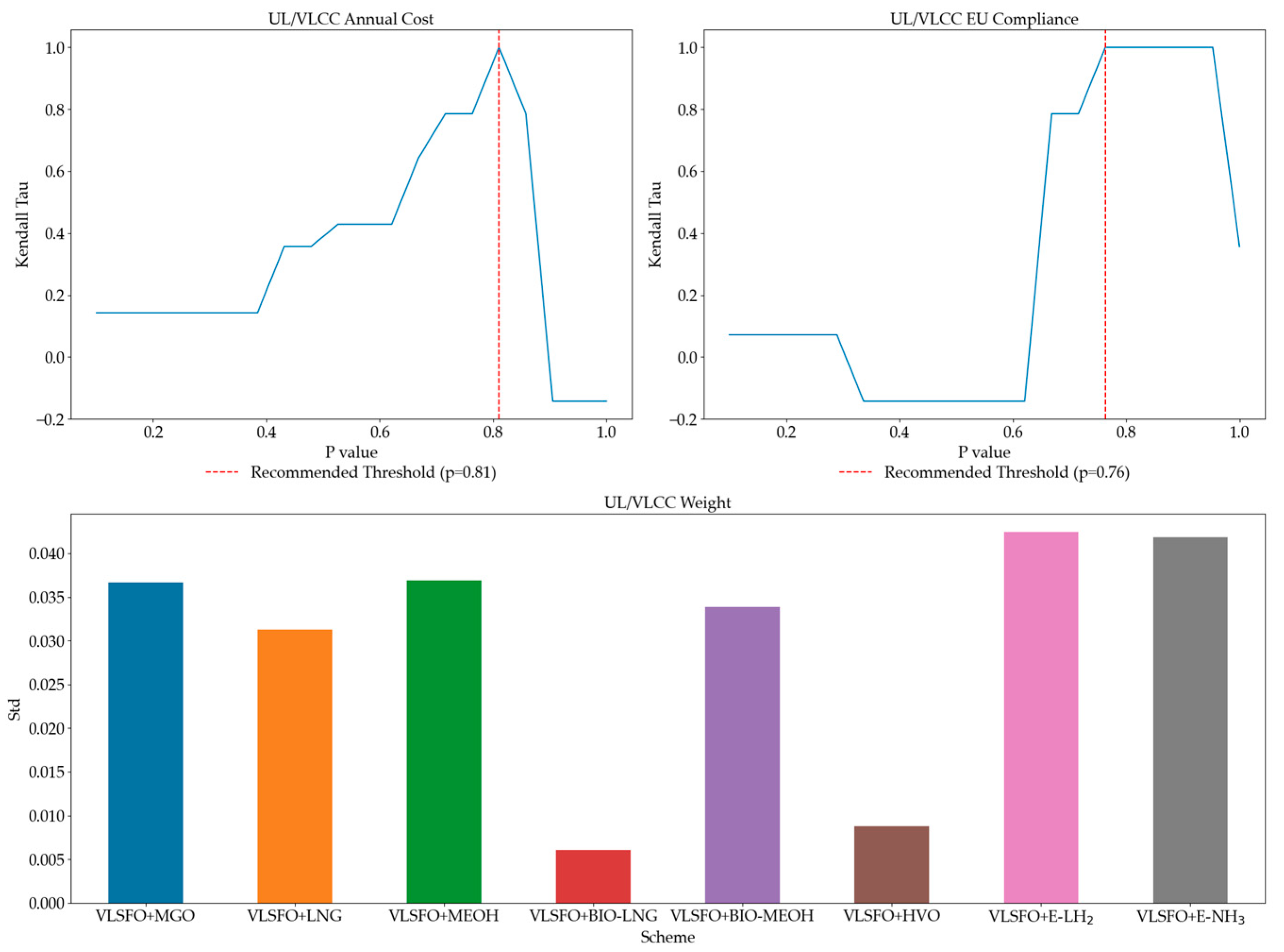
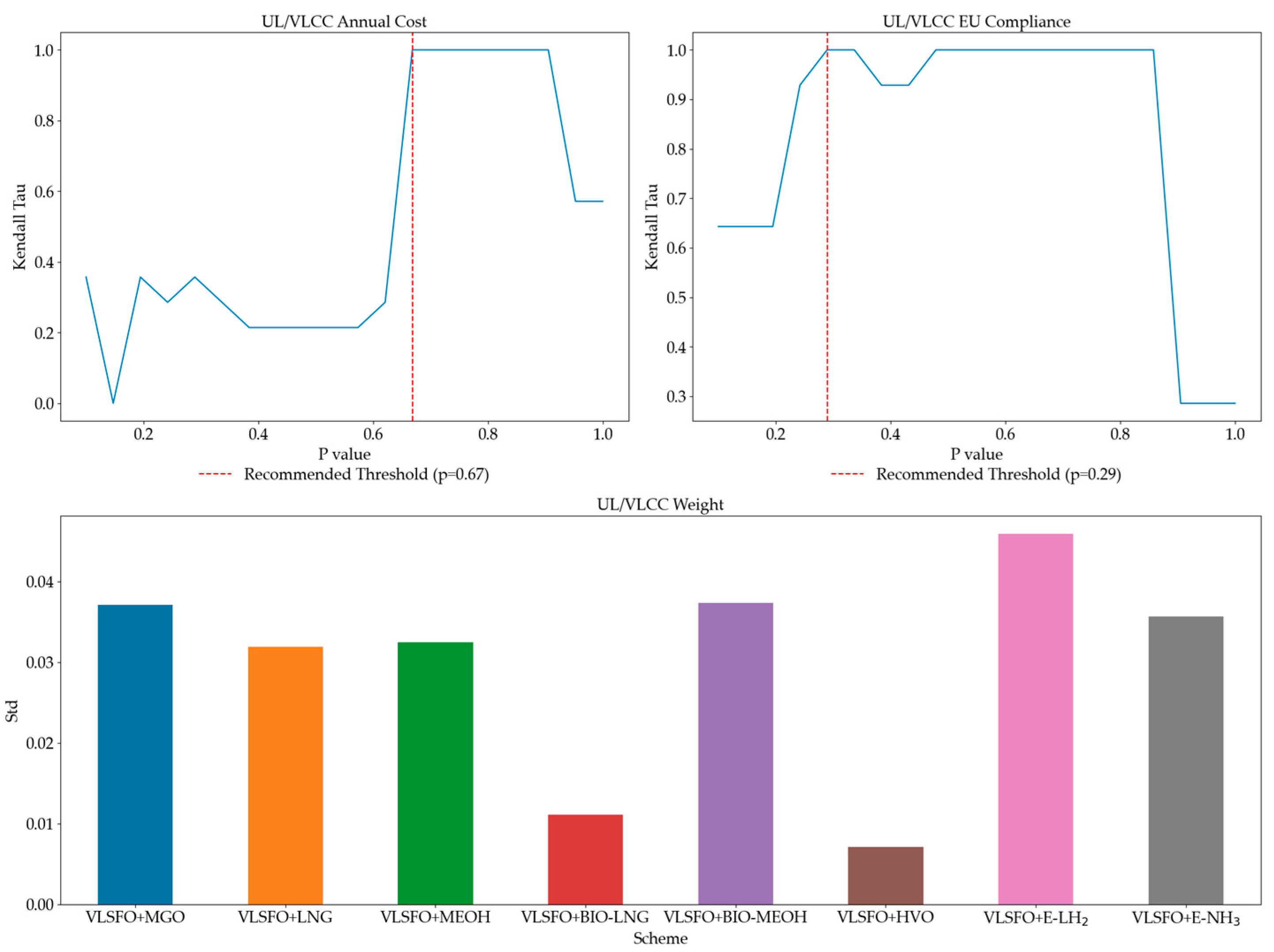
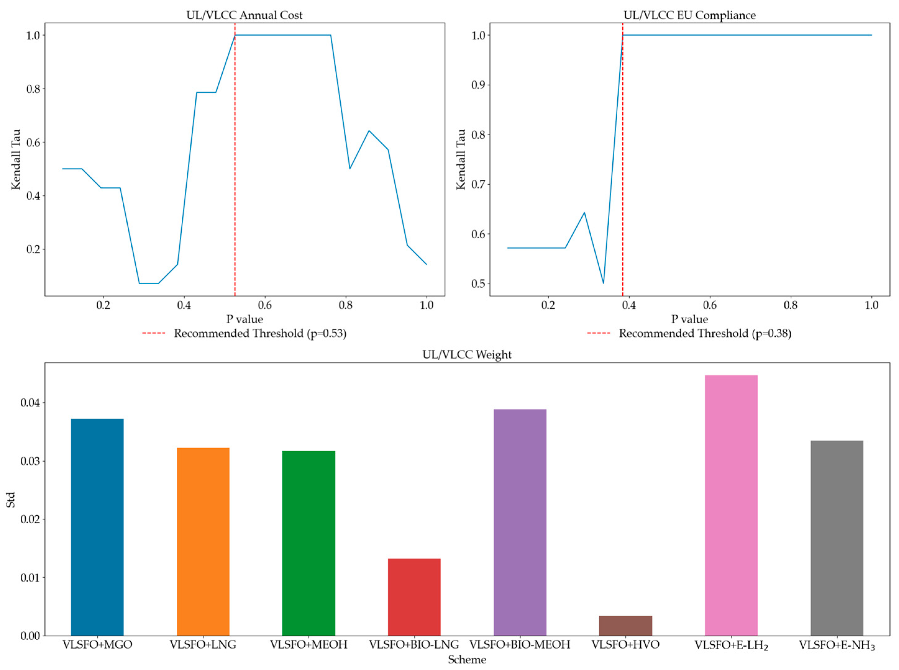
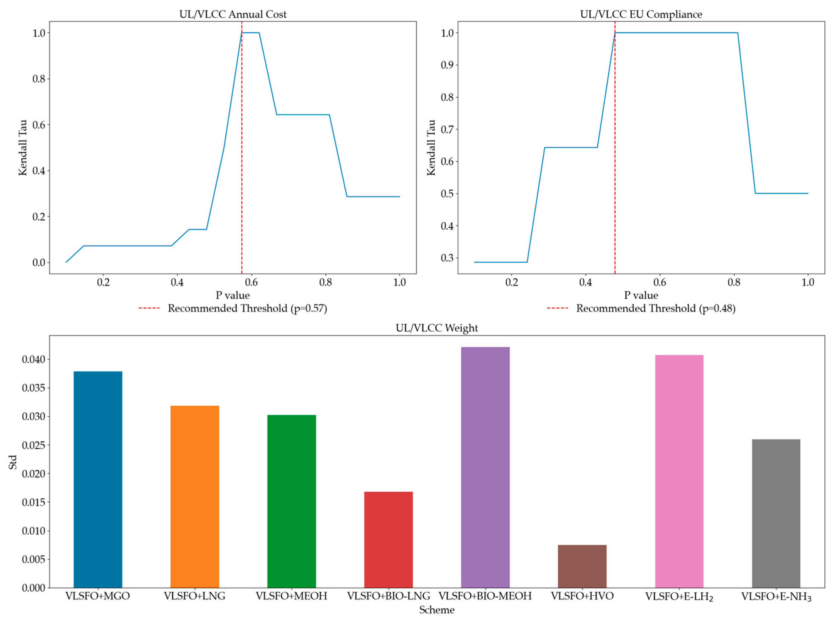
3.4. Sensitivity Analysis
4. Conclusions and Discussion
Author Contributions
Funding
Data Availability Statement
Conflicts of Interest
Nomenclature
| List of Abbreviations | |
| GHG | greenhouse gas |
| EU | European Union |
| WtW | well-to-wake |
| MCDA | multi-criteria decision analysis |
| VLSFO | very low sulfur fuel oil |
| MGO | marine gas oil |
| MEOH | methanol |
| E-LH2 | electrolytic liquid hydrogen |
| IMO | International Maritime Organization |
| ETS | Emissions Trading System |
| CO2 | carbon dioxide |
| CH4 | methane |
| N2O | nitrous oxide |
| LNG | liquefied natural gas |
| HVO | hydrotreated vegetable oil |
| LCA | life-cycle assessment |
| LCC | lLife-cycle cost |
| FT-diesel | Fischer–Tropsch diesel |
| TRL | technological readiness level |
| ETD | Energy Taxation Directive |
| LCV | lower calorific values |
| TtW | tank-to-wake |
| GWP | global warming potential |
| CAPEX | capital expenditure |
| EUR | euros |
| Symbols | |
| hourly fuel consumption of the main engine, t/h | |
| hourly fuel consumption of the auxiliary engine, t/h | |
| average sailing speed of the ship, kn | |
| design speed of the ship, kn | |
| design power of the main engine, kW | |
| specific fuel consumption of the main engine, g/kWh | |
| auxiliary engine load factor | |
| design power of the auxiliary engine, kW | |
| specific fuel consumption of the auxiliary engine, g/kWh | |
| annual consumption of alternative fuel for the main engine, t | |
| annual consumption of VLSFO for pilot fuel, t | |
| annual consumption of alternative fuel for the auxiliary engine, t | |
| lower calorific value of VLSFO, MJ/kg | |
| lower calorific value of the alternative fuel, MJ/kg | |
| lower calorific value of MGO, MJ/kg | |
| annual sailing time of the ship, h | |
| annual berthing time of the ship, h | |
| annual total consumption of alternative fuel, t | |
and | emission factors of CO2, CH4, and N2O released during combustion of alternative fuels in the main engine and auxiliary engine, gGHG/gFuel |
, and | emission factors of unburned methane and nitrous oxide leakage associated with alternative fuels in the main and auxiliary engines, gGHG/gFuel |
| the 100-year global warming potential values for CO2, CH4, and N2O | |
| annual well-to-tank GHG emission intensity, gCO2eq/MJ | |
| annual tank-to-wake GHG emission intensity, gCO2eq/MJ | |
| annual well-to-wake GHG emission intensity of the ship, gCO2eq/MJ | |
| fuel leakage rates for the main engine and auxiliary engine | |
| a key adjustment factor defined in the FuelEU Maritime regulation | |
| annual cost, € | |
| annualized capital investment cost, € | |
| fixed operating cost of the ship, € | |
| fuel-related variable operating cost, € | |
| opportunity cost associated with cargo space loss, € | |
| ship lifetime | |
| discount rate | |
| capital investment cost of the ship, € | |
| ratio of fixed operating cost to average annual shipbuilding cost | |
| price of the alternative fuel, € | |
| price of VLSFO, € | |
| cargo deadweight loss rate | |
| nominal container capacity of the containership | |
| unit cost per lost TEU, €/TEU/trip | |
| annual voyage frequency for containerships, trip | |
| deadweight tonnage of non-container ships | |
| unit cost per lost deadweight ton, €/tonne of space loss/h | |
| regulatory GHG intensity limit for energy used onboard the ship, gCO2eq/MJ | |
| calculated annual average GHG intensity of energy used onboard during the relevant reporting period, gCO2eq/MJ | |
| compliance balance, calculated as the absolute value of the difference between an | |
| the performance value of the alternative with respect to the criterion | |
| normalized value of the alternative with respect to the criterion | |
| sample standard deviation of criterion | |
| the mean value of criterion | |
| conflict measure of criterion with all other criteria | |
| correlation coefficient between criterion and criterion | |
| amount of information conveyed by criterion | |
| the final normalized weight of criterion | |
| the evaluation difference between alternative and alternative with respect to criterion | |
| the preference function for criterion | |
| the aggregated preference index of alternative over alternative | |
| the negative outranking flow | |
| the positive outranking flow | |
| the net outranking flow | |
Appendix A
References
- International Maritime Organization. Fourth Greenhouse Gas Study 2020. Available online: https://www.imo.org/en/OurWork/Environment/Pages/Fourth-IMO-Greenhouse-Gas-Study-2020.aspx (accessed on 20 April 2025).
- Vierth, I.; Ek, K.; From, E.; Lind, J. The cost impacts of Fit for 55 on shipping and their implications for Swedish freight transport. Transp. Res. Part A Policy Pract. 2024, 179, 103894. [Google Scholar] [CrossRef]
- International Maritime Organization. Revised GHG Reduction Strategy for Global Shipping Adopted. Available online: https://www.imo.org/en/MediaCentre/PressBriefings/pages/Revised-GHG-reduction-strategy-for-global-shipping-adopted-.aspx (accessed on 20 April 2025).
- DNV. FuelEU Maritime—Requirements, Compliance Strategies, and Commercial Impacts. Available online: https://www.dnv.com/maritime/publications/fueleu-maritime-white-paper-download/ (accessed on 27 February 2025).
- European Union. Official Journal of the European Union. Available online: https://eur-lex.europa.eu/legal-content/EN/TXT/?uri=OJ%3AL%3A2021%3A243%3ATOC (accessed on 20 April 2025).
- European Union. Fit for 55 Package. Available online: https://www.europarl.europa.eu/RegData/etudes/BRIE/2022/733513/EPRS_BRI(2022)733513_EN.pdf (accessed on 20 April 2025).
- European Commission. Decarbonising Maritime Transport—FuelEU Maritime. Available online: https://transport.ec.europa.eu/transport-modes/maritime/decarbonising-maritime-transport-fueleu-maritime_en (accessed on 27 February 2025).
- European Commission. Questions and Answers on Regulation (EU) 2023/1805 on the Use of Renewable and Low-Carbon Fuels in Maritime Transport, and AMENDING DIRECTIVE 2009/16/EC. Available online: https://transport.ec.europa.eu/transport-modes/maritime/decarbonising-maritime-transport-fueleu-maritime/questions-and-answers-regulation-eu-20231805-use-renewable-and-low-carbon-fuels-maritime-transport_en (accessed on 27 February 2025).
- MAN. MAN B&W ME-LGIP Dual-Fuel Engines. Available online: https://www.man-es.com/docs/default-source/document-sync-archive/b-w-me-lgip-dual-fuel-engines-dual-fuel-technology-reshapes-the-future-two-stroke-engine-operation-eng.pdf?sfvrsn=6e76dfc0_4 (accessed on 27 February 2025).
- Wang, Y.; Xiao, X.; Ji, Y. A Review of LCA Studies on Marine Alternative Fuels: Fuels, Methodology, Case Studies, and Recommendations. J. Mar. Sci. Eng. 2025, 13, 196. [Google Scholar] [CrossRef]
- Lee, H.; Lee, J.; Roh, G.; Lee, S.; Choung, C.; Kang, H. Comparative Life Cycle Assessments and Economic Analyses of Alternative Marine Fuels: Insights for Practical Strategies. Sustainability 2024, 16, 2114. [Google Scholar] [CrossRef]
- Xing, H.; Stuart, C.; Spence, S.; Chen, H. Alternative fuel options for low carbon maritime transportation: Pathways to 2050. J. Clean. Prod. 2021, 297, 126651. [Google Scholar] [CrossRef]
- Zincir, B. Environmental and economic evaluation of ammonia as a fuel for short-sea shipping: A case study. Int. J. Hydrogen Energy 2022, 47, 18148–18168. [Google Scholar] [CrossRef]
- Ratnakar, R.R.; Gupta, N.; Zhang, K.; van Doorne, C.; Fesmire, J.; Dindoruk, B.; Balakotaiah, V. Hydrogen supply chain and challenges in large-scale LH2 storage and transportation. Int. J. Hydrogen Energy 2021, 46, 24149–24168. [Google Scholar] [CrossRef]
- Ishaq, H.; Crawford, C. Review of ammonia production and utilization: Enabling clean energy transition and net-zero climate targets. Energy Convers. Manag. 2024, 300, 117869. [Google Scholar] [CrossRef]
- Brouzas, S.; Zadeh, M.; Lagemann, B. Essentials of hydrogen storage and power systems for green shipping. Int. J. Hydrogen Energy 2025, 100, 1543–1560. [Google Scholar] [CrossRef]
- Bui, K.Q.; Perera, L.P.; Emblemsvåg, J. Life-cycle cost analysis of an innovative marine dual-fuel engine under uncertainties. J. Clean. Prod. 2022, 380, 134847. [Google Scholar] [CrossRef]
- Law, L.C.; Foscoli, B.; Mastorakos, E.; Evans, S. A Comparison of Alternative Fuels for Shipping in Terms of Lifecycle Energy and Cost. Energies 2021, 14, 8502. [Google Scholar] [CrossRef]
- Solakivi, T.; Paimander, A.; Ojala, L. Cost competitiveness of alternative maritime fuels in the new regulatory framework. Transp. Res. Part D Transp. Environ. 2022, 113, 103500. [Google Scholar] [CrossRef]
- Flodén, J.; Lars, Z.; Anastasia, C.; Rasmus, P.; Erik, F.; Julia, H.; Johan, R.; Woxenius, J. Shipping in the EU emissions trading system: Implications for mitigation, costs and modal split. Clim. Policy 2024, 24, 969–987. [Google Scholar] [CrossRef]
- Trosvik, L.; Brynolf, S. Decarbonising Swedish maritime transport: Scenario analyses of climate policy instruments. Transp. Res. Part D Transp. Environ. 2024, 136, 104457. [Google Scholar] [CrossRef]
- Deniz, C.; Zincir, B. Environmental and economical assessment of alternative marine fuels. J. Clean. Prod. 2016, 113, 438–449. [Google Scholar] [CrossRef]
- Ren, J.; Liang, H. Measuring the sustainability of marine fuels: A fuzzy group multi-criteria decision making approach. Transp. Res. Part D Transp. Environ. 2017, 54, 12–29. [Google Scholar] [CrossRef]
- Soltani Motlagh, H.R.; Issa Zadeh, S.B.; Garay-Rondero, C.L. Towards International Maritime Organization Carbon Targets: A Multi-Criteria Decision-Making Analysis for Sustainable Container Shipping. Sustainability 2023, 15, 16834. [Google Scholar] [CrossRef]
- Moshiul, A.M.; Mohammad, R.; Hira, F.A. Alternative Fuel Selection Framework toward Decarbonizing Maritime Deep-Sea Shipping. Sustainability 2023, 15, 5571. [Google Scholar] [CrossRef]
- Strantzali, E.; Livanos, G.A.; Aravossis, K. A Comprehensive Multicriteria Evaluation Approach for Alternative Marine Fuels. Energies 2023, 16, 7498. [Google Scholar] [CrossRef]
- Zou, J.; Yang, B. Evaluation of alternative marine fuels from dual perspectives considering multiple vessel sizes. Transp. Res. Part D Transp. Environ. 2023, 115, 103583. [Google Scholar] [CrossRef]
- Fan, L.; Gu, B.; Luo, M. A cost-benefit analysis of fuel-switching vs. hybrid scrubber installation: A container route through the Chinese SECA case. Transp. Policy 2020, 99, 336–344. [Google Scholar] [CrossRef]
- European Commission. Regulation (EU) 2023/1805 of the European Parliament and of the Council of 13 September 2023 on the Use of Renewable and Low-Carbon Fuels in Maritime Transport, and Amending Directive 2009/16/EC (Text with EEA relevance). Available online: https://eur-lex.europa.eu/legal-content/EN/TXT/?uri=CELEX%3A32023R1805#ntr4-L_2023234EN.01004801-E0004 (accessed on 27 February 2025).
- European Commission. Directive (EU) 2018/2001 of the European Parliament and of the Council of 11 December 2018 on the Promotion of the Use of Energy from Renewable Sources (Recast) (Text with EEA Relevance.). Available online: https://eur-lex.europa.eu/eli/dir/2018/2001/oj/eng (accessed on 27 February 2025).
- Zhang, W.; He, Y.; Wu, N.; Zhang, F.; Lu, D.; Liu, Z.; Jing, R.; Zhao, Y. Assessment of cruise ship decarbonization potential with alternative fuels based on MILP model and cabin space limitation. J. Clean. Prod. 2023, 425, 138667. [Google Scholar] [CrossRef]
- Wang, Y.; Wright, L.A. A Comparative Review of Alternative Fuels for the Maritime Sector: Economic, Technology, and Policy Challenges for Clean Energy Implementation. World 2021, 2, 456–481. [Google Scholar] [CrossRef]
- Tran, N.K.; Haasis, H.-D. An empirical study of fleet expansion and growth of ship size in container liner shipping. Int. J. Prod. Econ. 2015, 159, 241–253. [Google Scholar] [CrossRef]
- Behzadian, M.; Kazemzadeh, R.B.; Albadvi, A.; Aghdasi, M. PROMETHEE: A comprehensive literature review on methodologies and applications. Eur. J. Oper. Res. 2010, 200, 198–215. [Google Scholar] [CrossRef]
- Diakoulaki, D.; Mavrotas, G.; Papayannakis, L. Determining objective weights in multiple criteria problems: The critic method. Comput. Oper. Res. 1995, 22, 763–770. [Google Scholar] [CrossRef]
- Brans, J.P.; Vincke, P. Note—A Preference Ranking Organisation Method. Manag. Sci. 1985, 31, 647–656. [Google Scholar] [CrossRef]
- Ship & Bunker. Integr8: VLSFO Calorific Value, Pour Point and Competitiveness with LSMGO. Available online: https://shipandbunker.com/news/world/662089-integr8-vlsfo-calorific-value-pour-point-and-competitiveness-with-lsmgo (accessed on 23 March 2025).
- Sustainable Ships. FuelEU Maritime Guide. Available online: https://www.sustainable-ships.org/rules-regulations/fueleu (accessed on 23 March 2025).
- International Maritime Organization. Guidelines on Life Cycle GHG Intensity of Marine Fuels. Available online: https://wwwcdn.imo.org/localresources/en/OurWork/Environment/Documents/annex/MEPC%2080/Annex%2014.pdf (accessed on 23 March 2025).
- Lindstad, E.; Lagemann, B.; Rialland, A.; Gamlem, G.M.; Valland, A. Reduction of maritime GHG emissions and the potential role of E-fuels. Transp. Res. Part D Transp. Environ. 2021, 101, 103075. [Google Scholar] [CrossRef]
- Ashrafi, M.; Lister, J.; Gillen, D. Toward a harmonization of sustainability criteria for alternative marine fuels. Marit. Transp. Res. 2022, 3, 100052. [Google Scholar] [CrossRef]
- MAN. The Benefits of Methanol. Available online: https://www.man-es.com/discover/the-benefits-of-methanol (accessed on 23 March 2025).
- DNV. Biofuels in Shipping—Current Market and Guidance on Use and Reporting. Available online: https://www.dnv.com/maritime/publications/Biofuels-in-shipping-white-paper-2025-download/ (accessed on 23 March 2025).
- Wang, Y.; Cao, Q.; Liu, L.; Wu, Y.; Liu, H.; Gu, Z.; Zhu, C. A review of low and zero carbon fuel technologies: Achieving ship carbon reduction targets. Sustain. Energy Technol. Assess. 2022, 54, 102762. [Google Scholar] [CrossRef]
- Lagemann, B.; Lagouvardou, S.; Lindstad, E.; Fagerholt, K.; Psaraftis, H.N.; Erikstad, S.O. Optimal ship lifetime fuel and power system selection under uncertainty. Transp. Res. Part D Transp. Environ. 2023, 119, 103748. [Google Scholar] [CrossRef]
- Clarksons Research. Shipping Intelligence Weekly 20/12/2024. Available online: https://www.clarksons.net.cn/api/download/SIN/download/718365d9-1918-4b7b-91fb-b92ba474fd91?downloadInline=true (accessed on 27 March 2025).
- Korberg, A.D.; Brynolf, S.; Grahn, M.; Skov, I.R. Techno-economic assessment of advanced fuels and propulsion systems in future fossil-free ships. Renew. Sustain. Energy Rev. 2021, 142, 110861. [Google Scholar] [CrossRef]
- ABS. View of The Value Chain. Available online: https://absinfo.eagle.org/acton/attachment/16130/f-c04f4eaf-a121-4560-9e15-5a56ee443f32/1/-/-/-/-/sustainability-outlook-iii-21055-web.pdf (accessed on 27 March 2025).
- Methanol Institute. Economic Value of Methanol for Shipping Under FuelEU Maritime and EU ETS. Available online: https://www.methanol.org/wp-content/uploads/2024/09/ECONOMIC-VALUE-OF-METHANOL-FOR-SHIPPING-PAPER_final.pdf (accessed on 27 March 2025).
- Lorenzi, G.; Baptista, P.; Venezia, B.; Silva, C.; Santarelli, M. Use of waste vegetable oil for hydrotreated vegetable oil production with high-temperature electrolysis as hydrogen source. Fuel 2020, 278, 117991. [Google Scholar] [CrossRef]
- ABS. Beyond the Horizon: Carbon Neutral Fuel Pathways and Transformational Technologies. Available online: https://ww2.eagle.org/en/interactive/interactive-publications/current/outlook-2024.html (accessed on 27 March 2025).
- Hansson, J.; Månsson, S.; Brynolf, S.; Grahn, M. Alternative marine fuels: Prospects based on multi-criteria decision analysis involving Swedish stakeholders. Biomass Bioenergy 2019, 126, 159–173. [Google Scholar] [CrossRef]
- Notteboom, T.E.; Vernimmen, B. The effect of high fuel costs on liner service configuration in container shipping. J. Transp. Geogr. 2009, 17, 325–337. [Google Scholar] [CrossRef]


| Ship Category | Ship Subtype | DWT/ TEU | Main Engine Power (kW) | Auxiliary Engine Power (kW) | Design Speed (kn) | Average Speed (kn) | Sailing Time Within EU Waters (h) | Berthing Time at EU Ports (h) | Newbuilding Price (Million EUR) |
|---|---|---|---|---|---|---|---|---|---|
| Tanker | UL/VLCC | 296,174 | 22,200 | 4620 | 14.8 | 11.4 | 4913 | 529 | 115.92 |
| Suezmax | 147,630 | 18,200 | 4400 | 14.0 | 11.8 | 3963 | 2487 | 80.96 | |
| Aframax | 108,553 | 14,070 | 2310 | 15.3 | 9.9 | 1630 | 858 | 68.54 | |
| Panamax | 71,573 | 22,400 | 4200 | 16.0 | 9.8 | 5453 | 3410 | 54.74 | |
| Handysize | 37,993 | 9960 | 1776 | 14.2 | 11.2 | 4110 | 3662 | 45.08 | |
| Small tanker | 6870 | 2400 | 945 | 10.0 | 8 | 4272 | 4585 | 16.56 | |
| Bulker | Capesize | 181,709 | 18,660 | 2400 | 11.5 | 10.8 | 579 | 486 | 68.08 |
| Panamax | 81,290 | 9930 | 2400 | 14.3 | 11.1 | 2461 | 1237 | 34.04 | |
| Handymax | 82,094 | 9710 | 2400 | 14.0 | 10.9 | 984 | 1247 | 34.04 | |
| Handysize | 21,353 | 9720 | 2400 | 17.5 | 10 | 3092 | 3942 | 19.32 | |
| Containership | Post-Panamax | 18,270 | 59,360 | 15,000 | 19.0 | 15.3 | 2649 | 773 | 196.42 |
| Neo-Panamax | 14,074 | 72,240 | 13,790 | 24.2 | 15.1 | 3921 | 698 | 140.76 | |
| Intermediate | 6750 | 57,099 | 9000 | 25.5 | 15.8 | 2769.5 | 1242 | 81.88 | |
| General Cargo | General Cargo I | 9500 | 4000 | 1030 | 13.0 | 10.7 | 3312 | 1491 | 17.00 |
| General Cargo II | 10,952 | 3360 | 1170 | 12.0 | 10.5 | 2031 | 1605 | 17.94 | |
| Ferry | Ro-Pax | 12,662 | 33,600 | 5850 | 23.0 | 17.5 | 4759.12 | 3473.9 | 60.68 |
| Pass/Car | 6133 | 31,200 | 7840 | 21.0 | 19 | 6567.71 | 1803 | 45.25 |
| Fuel Type | LCV (MJ/kg) | WtT Emission Factor (gCO2eq/MJ) | TtW Emission Factor | Newbuilding Price Adjustment Factor | Cargo Deadweight Loss Rate for This Fuel (%) | ||
|---|---|---|---|---|---|---|---|
| (CO2 gCO2eq/g Fuel) | CH4 (gCH4eq/g Fuel) | N2O (gN2Oeq/g Fuel) | |||||
| VLSFO | 41 [37] | 13.2 [38] | 3.114 [39] | 0.00005 [39] | 0.00018 [39] | 1 | – |
| MGO | 42.7 [38] | 14.4 [38] | 3.206 [39] | 0.00005 [39] | 0.00018 [39] | 1 | – |
| LNG | 49.1 [38] | 18.5 [40] | 2.750 [39] | 0 [39] | 0.00011 [39] | 1.23 [41] | 1 [27] |
| MEOH | 19.9 [38] | 31.3 [40] | 1.375 [38] | 0 [38] | 0.00018 [38] | 1.1 [42] | 2 [27] |
| Bio-LNG | 50 [19] | −25 [38] | 2.750 [38] | 0 [38] | 0.00011 [38] | 1.23 [41] | 1 [27] |
| Bio-MEOH | 20 [38] | −55.4 [38] | 1.375 [38] | 0 [38] | 0.00018 [38] | 1.1 [42] | 2 [27] |
| HVO | 44 [19] | −33.4 [38] | 3.115 [38] | 0.00005 [38] | 0.00018 [38] | 1 [43] | – |
| E-LH2 | 120 [44] | 0 [40] | 0 [39] | 0 [38] | 0.00018 [38] | 1.58 [45] | 5 [27] |
| E-NH3 | 18.6 [38] | 0 [40] | 0 [40] | 0 [38] | 0.00018 [38] | 1.25 [45] | 3 [27] |
| Voyage Length | Short | Medium | Long |
|---|---|---|---|
| Tanker (€/dwt/day) | 0.59 [46] | 0.33 [46] | 0.12 [46] |
| Bulker (€/dwt/day) | 0.30 [46] | 0.21 [46] | 0.08 [46] |
| Ferry (€/m3 of space loss) | 6 [47] | 8 [47] | 10 [47] |
| General cargo (€/dwt/day) | 0.1 [47] | – | – |
| Containership (€/TEU/trip) | 600 [47] | 900 [47] | 1100 [47] |
| Year | GHG Intensity Target | Fuel Price (EUR/t) | ||||||||
|---|---|---|---|---|---|---|---|---|---|---|
| VLSFO | MGO | LNG | MEOH | Bio-LNG | Bio-MEOH | HVO | E-LH2 | E-NH3 | ||
| 2025 | 89.34 | 540.14 | 731.5 | 543.60 [4] | 460 [48] | 1383.90 [4] | 1193 [49] | 1000 [50] | 5059.54 [51] | 1072.52 [51] |
| 2030 | 85.69 | 514.46 | 847 | 665.03 | 575 | 1231 | 1152 | 1031.12 | 5299.2 | 872.71 |
| 2035 | 77.94 | 692.58 | 885 | 715.22 | 582 | 1138.5 | 1147.5 | 1177.86 | 4857.6 | 804.26 |
| 2040 | 62.90 | 870.7 | 923 | 752.87 | 589 | 1046 | 1143 | 1324.6 | 4416 | 735.82 |
| 2045 | 34.64 | 1015.30 | 935.5 | 790.51 | 585.5 | 980 | 1125 | 1467.97 | 3974.4 | 663 |
| 2050 | 18.23 | 1159.89 | 948 | 828.15 | 582 | 914 | 1107 | 1611.33 | 3532.8 | 590.36 |
| Ship/Year | 2025 | 2030 | 2035 | 2040 | 2045 | 2050 |
|---|---|---|---|---|---|---|
| UL/VLCC | VLSFO + HVO | VLSFO + HVO | VLSFO + HVO | VLSFO + HVO | VLSFO + BIO-LNG | VLSFO + E-NH3 |
| Suezmax | VLSFO + HVO | VLSFO + HVO | VLSFO + HVO | VLSFO + BIO-LNG | VLSFO + BIO-LNG | VLSFO + E-NH3 |
| Aframax | VLSFO + HVO | VLSFO + HVO | VLSFO + HVO | VLSFO + HVO | VLSFO + HVO | VLSFO + HVO |
| Panamax | VLSFO + HVO | VLSFO + HVO | VLSFO + HVO | VLSFO + BIO-LNG | VLSFO + BIO-LNG | VLSFO + E-LH2 |
| Handysize | VLSFO + HVO | VLSFO + HVO | VLSFO + HVO | VLSFO + HVO | VLSFO + BIO-LNG | VLSFO + E-NH3 |
| Small tanker | VLSFO + HVO | VLSFO + HVO | VLSFO + HVO | VLSFO + HVO | VLSFO + BIO-LNG | VLSFO + E-NH3 |
| Capesize | VLSFO + HVO | VLSFO + HVO | VLSFO + HVO | VLSFO + HVO | VLSFO + HVO | VLSFO + E-NH3 |
| Panamax | VLSFO + HVO | VLSFO + HVO | VLSFO + HVO | VLSFO + HVO | VLSFO + BIO-LNG | VLSFO + E-NH3 |
| Handymax | VLSFO + HVO | VLSFO + HVO | VLSFO + HVO | VLSFO + HVO | VLSFO + HVO | VLSFO + E-NH3 |
| Handysize | VLSFO + HVO | VLSFO + HVO | VLSFO + HVO | VLSFO + BIO-LNG | VLSFO + BIO-LNG | VLSFO + E-NH3 |
| Post-Panamax | VLSFO + HVO | VLSFO + HVO | VLSFO + HVO | VLSFO + HVO | VLSFO + BIO-LNG | VLSFO + E-NH3 |
| Neo-Panamax | VLSFO + HVO | VLSFO + HVO | VLSFO + HVO | VLSFO + BIO-LNG | VLSFO + BIO-LNG | VLSFO + E-NH3 |
| Intermediate | VLSFO + HVO | VLSFO + HVO | VLSFO + HVO | VLSFO + HVO | VLSFO + BIO-LNG | VLSFO + BIO-LNG |
| General Cargo I | VLSFO + HVO | VLSFO + HVO | VLSFO + HVO | VLSFO + HVO | VLSFO + BIO-LNG | VLSFO + E-NH3 |
| General Cargo II | VLSFO + HVO | VLSFO + HVO | VLSFO + HVO | VLSFO + HVO | VLSFO + E-NH3 | VLSFO + E-NH3 |
| Ro-Pax | VLSFO + HVO | VLSFO + HVO | VLSFO + HVO | VLSFO + E-LH2 | VLSFO + E-LH2 | VLSFO + E-LH2 |
| Pass/Car | VLSFO + E-LH2 | VLSFO + HVO | VLSFO + E-LH2 | VLSFO + E-LH2 | VLSFO + E-LH2 | VLSFO + E-LH2 |
Disclaimer/Publisher’s Note: The statements, opinions and data contained in all publications are solely those of the individual author(s) and contributor(s) and not of MDPI and/or the editor(s). MDPI and/or the editor(s) disclaim responsibility for any injury to people or property resulting from any ideas, methods, instructions or products referred to in the content. |
© 2025 by the authors. Licensee MDPI, Basel, Switzerland. This article is an open access article distributed under the terms and conditions of the Creative Commons Attribution (CC BY) license (https://creativecommons.org/licenses/by/4.0/).
Share and Cite
Wang, C.; Peng, Z.; Yang, J.; Zhang, N.; Li, K.; Li, X. Optimal Alternative Fuel Selection for Dual-Fuel Ships Under FuelEU Maritime Regulations: Environmental and Economic Assessment. J. Mar. Sci. Eng. 2025, 13, 1105. https://doi.org/10.3390/jmse13061105
Wang C, Peng Z, Yang J, Zhang N, Li K, Li X. Optimal Alternative Fuel Selection for Dual-Fuel Ships Under FuelEU Maritime Regulations: Environmental and Economic Assessment. Journal of Marine Science and Engineering. 2025; 13(6):1105. https://doi.org/10.3390/jmse13061105
Chicago/Turabian StyleWang, Cong, Zhongxiu Peng, Jianming Yang, Niyu Zhang, Ke Li, and Xuesong Li. 2025. "Optimal Alternative Fuel Selection for Dual-Fuel Ships Under FuelEU Maritime Regulations: Environmental and Economic Assessment" Journal of Marine Science and Engineering 13, no. 6: 1105. https://doi.org/10.3390/jmse13061105
APA StyleWang, C., Peng, Z., Yang, J., Zhang, N., Li, K., & Li, X. (2025). Optimal Alternative Fuel Selection for Dual-Fuel Ships Under FuelEU Maritime Regulations: Environmental and Economic Assessment. Journal of Marine Science and Engineering, 13(6), 1105. https://doi.org/10.3390/jmse13061105