Abstract
Construction sites with deep soft deposits usually experience significant consolidation settlement that can compromise structural integrity if not properly monitored. Conventional methods, such as settlement plates, are limited by high costs and sparse spatial coverage, which leaves areas unmonitored and vulnerable to unexpected settlement. Therefore, this study develops an integrated UAV LiDAR monitoring framework that optimizes data preprocessing and introduces a novel timeseries settlement correction and interpolation technique for staged surcharge loading. Using UAV LiDAR data acquired at biweekly intervals from May 2021 to March 2022 at Busan Newport, high-quality digital elevation models were generated through optimal preprocessing. We are the first to evaluate the spatial representativeness of consolidation settlement at multiple section sizes (10 m × 10 m, 50 m × 50 m, and 100 m × 100 m) using high-resolution LiDAR, revealing that larger section sizes produce greater spatial variability and prediction error. Moreover, we demonstrate that at least seven biweekly UAV LiDAR surveys are essential to reliably capture early-stage settlement behaviors, providing a practical guideline for monitoring campaigns. These findings show that the proposed UAV LiDAR framework can deliver valuable insights for managing settlement in marine and soft ground construction projects.
1. Introduction
Consolidation settlement is a phenomenon where the volume of soil decreases, and deformation that occurs as pore water within the ground is expelled due to external loads. In general, soft ground consists of fine clay particles with very low permeability. This condition causes the consolidation process to progress very slowly, which ultimately results in large settlement. In particular, soft ground, such as dredged and reclaimed soil in coastal areas, has high compressibility and low shear strength, which leads to the possibility of excessive long-term settlement [1,2].
When large-scale structures, such as ports and bridges, are built on deep soft ground, prolonged post-construction settlement can lead to differential settlement. These issues can ultimately lead to serious structural stability problems, including tilting and cracking of the structures. For instance, in Busan Newport, South Korea, a differential settlement of up to 0.1 m has been reported. Accurately predicting settlement is essential for minimizing residual settlement and ensuring long-term structural integrity to mitigate the aforementioned risks.
Settlement prediction in soft ground sites is performed during the design and construction phases. The design phase aims to predict settlement over time during the initial planning process to incorporate it into construction plans and structural design. The construction phase focuses on effectively managing settlement through predictions using actual measurement data.
In the design phase, various consolidation theories [3,4,5,6,7,8,9,10] and numerical analysis approaches are adapted [11,12] to accurately predict the settlement. However, applying these methods is challenging in practice due to their complex mathematical derivations [10]. Furthermore, differences between predictions and actual measurements frequently occur due to the variability of soil parameters and complex field characteristics.
In the construction phase, settlement is re-predicted based on observational methods to enhance the accuracy of settlement predictions. These methods incorporate actual measurements collected from settlement plates. The observational method includes several representative techniques, including the hyperbolic method [13,14], the Asaoka method [15], and the weighted nonlinear regression hyperbolic method [16,17].
Previous studies have demonstrated that the observational methods are highly accurate in predicting settlement when an efficient amount of data are provided [18,19,20]. However, in large-scale sites, settlement plates are limitedly placed due to economic issues. This limitation allows only local settlement to be confirmed, which increases the possibility of problems, such as differential settlement.
UAV LiDAR technology has recently attracted attention in the geotechnical field for addressing the abovementioned issues [21]. UAV LiDAR provides high-resolution precise data over wide areas, which play an important role in analyzing and predicting settlement behavior [22]. Even in areas including forestry, archaeology, and disaster management, studies have used UAV LiDAR technology to overcome limitations in practical methods [23,24,25].
In particular, UAV LiDAR can effectively acquire precise data in environments with significant temporal changes in topography, such as soft ground and coastal areas [26,27,28,29,30]. The collected data have high accuracy within a few centimeters and can be used to analyze complex deformation patterns that are difficult to grasp with existing point-based measurement methods [31,32].
These data are used not only for local deformation assessment but also for verifying the effects of ground improvement techniques, such as preloading [33]. However, several challenges remain in long-term settlement monitoring and analysis using UAV LiDAR technology. For example, processes such as noise removal, vegetation and material removal from point cloud data are essential tasks to ensure data reliability [31,34]. In addition, data modeling that reflects changes in surcharge fill and layer conditions during ground improvement is necessary. Settlement behavior prediction results based on UAV LiDAR can become more precise through such optimization processes.
Despite these developments, several critical gaps persist. First, conventional monitoring approaches, such as settlement plates and GPS leveling, provide only discrete, point-based measurements, leaving most of the area unmonitored and failing to capture the true spatial variability of consolidation settlement. Second, although remote sensing and UAV platforms have advanced rapidly, their application to soft-ground consolidation monitoring remains in its infancy with key processing challenges. Noise removal, grid-size optimization, and robust bare-earth filtering have not been addressed in a unified framework. Third, prior studies have not thoroughly evaluated the field accuracy of UAV-based settlement predictions under realistic site conditions.
To fill these gaps, our work presents a comprehensive UAV LiDAR framework that delivers dense spatial coverage, integrates customized data-processing workflows, applies timeseries corrections for staged loading, and validates settlement predictions through detailed performance metrics.
Moreover, the study site at Busan Newport in South Korea represents a marine reclamation project for a major port facility constructed on land reclaimed from dredged soils. In such reclaimed coastal ground, large consolidation and differential settlement pose inherent marine geotechnical challenges to port yards, quay walls, and other coastal infrastructure [35,36]. The framework presented herein can be directly applied to monitor settlement across these reclamation sites, enabling the early detection of anomalous deformation and thereby preventing structural failures in marine construction projects.
Therefore, this study developed a UAV LiDAR-based framework for consolidation settlement monitoring and spatial analysis. The database was built based on UAV LiDAR measurement data conducted at 2-week intervals from May 2021 to March 2022 in Busan Newport. The proposed approach comprises three main components. First, optimal data preprocessing is performed by integrating denoising, grid size optimization, and bare-earth filtering to generate high-quality DEMs. Second, an innovative settlement evaluation method that incorporates timeseries corrections and interpolation techniques is applied to accurately capture surcharge fill and consolidation settlement. Third, comparative analyses across various grid sizes are conducted to assess the spatial representativeness of UAV LiDAR data against conventional settlement plate measurements. This integrated approach provides a new perspective for monitoring settlement in deep soft ground and establishes a robust framework for advanced consolidation monitoring.
2. Study Site
2.1. Overview of the Study Site and Geotechnical Characteristics
Figure 1 illustrates the location of the study site in Busan Newport, South Korea. The site underwent extensive reclamation during the 1980s to establish a large container terminal. This reclamation process used stones, sand, and marine clay to expand the land. Following reclamation and a resting period, ground improvement methods were applied to reduce settlement and strengthen the ground. On the eastern side of the study site, deep cement mixing techniques (DCM) were implemented, while preloading was applied on the western side. This study focuses on the west side of the study site where preloading was applied, and the site is defined as the study area.
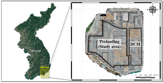
Figure 1.
Location of the study site in Busan Newport.
Figure 2 presents the location of the boreholes and the settlement plates within the study site. The boreholes were used for geotechnical investigation, while the settlement plates were installed to monitor the settlement during construction. Soil samples were collected from the boreholes, and laboratory tests were performed to determine the strength, properties, and profile of the ground. Laboratory tests included oedometer tests, unconfined compressive strength tests (UCS), and triaxial tests. Field tests including standard penetration tests (SPT) and flat dilatometer tests (DMT) were conducted to determine the strength of the ground further.
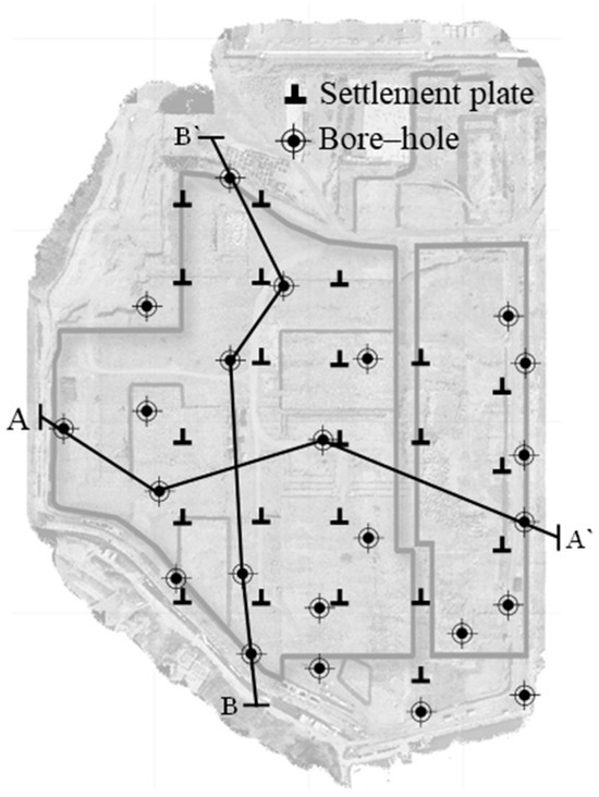
Figure 2.
Bore holes and settlement plates in the study site.
Figure 3 shows the soil profile across cross sections A-A’ and B-B’. In section A-A’, as shown in Figure 3a, a clay layer extends to a depth of around 45 m, with a thin gravel layer within it, followed by layers of sand, gravel, and rock. This clay layer is divided into a reclamation layer and a sedimentary layer; the reclamation layer reaches from the surface down to approximately 10 m, while the sedimentary layer continues from 10 m to 45 m. Figure 3b displays a similar profile in section B-B’, where the clay layer also extends to approximately 45 m, underlain by gravel, sand, and rock layers. In this section, the clay layer is similarly divided, with the reclamation layer ranging from the surface to 7.5 m and the sedimentary layer extending from 7.5 m to 45 m.
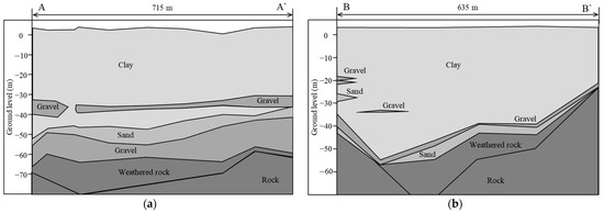
Figure 3.
Soil profiles of the study site: (a) cross section A-A’; (b) cross section B-B’.
Figure 4 depicts the soil strength and properties according to depth. In Figure 4a, the SPT-N values are presented; they indicate soft layers with SPT-N values below 6 up to a depth of 40 m, followed by a significant increase. Figure 4b shows the undrained shear strength (Su) determined from laboratory and field tests. Su increased linearly with depth and showed a notable transition beyond 20 m.
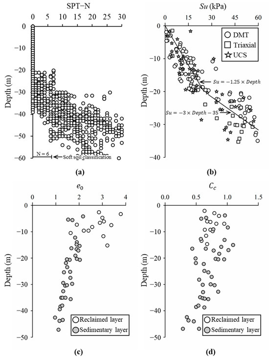
Figure 4.
Soil strength and properties of the study site: (a) SPT-N according to depth; (b) Su according to depth; (c) eo according to depth; (d) Cc according to depth.
Figure 4c,d presents the distribution of the initial void ratio (eo) and compression index (Cc) with respect to depth. The data points in these figures are categorized into the following two distinct layers: the reclaimed layer and the sedimentary layer. Within the reclaimed layer, the average eo was found to be 2.70, while the average Cc was 0.74. By contrast, the sedimentary layer exhibited lower values, with an average eo of 1.56 and an average Cc of 0.68. Across all data, the eo ranged from approximately 1.0 to 3.8 (mean = 2.4, standard deviation = 0.81), and the Cc ranged from about 0.3 to 1.1 (mean = 0.7, standard deviation = 0.23), confirming the highly compressible nature of the site soils and providing quantitative context for the magnitude of the observed settlement.
2.2. Measurements
Figure 5 shows the UAV LiDAR used in this study. UAV LiDAR is a remote sensing method that uses laser light to measure distances and create detailed 3D representations of the surface. LiDAR transmits light in the form of lasers to objects and analyzes the returned signal to derive the distance. The result is a point cloud, which is a set of measured points that can be connected to create a surface representation of an object.
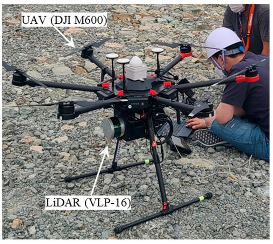
Figure 5.
UAV LiDAR used in this study.
In this study, UAV LiDAR measurements were conducted 19 times at biweekly intervals from May 2021 to March 2022. Measurements were not conducted during snowy or rainy conditions to avoid errors caused by water on the ground.
The UAV LiDAR equipment consisted of a DJI M600 drone (DJI, Shenzhen, China), an Applanix 15 GNSS/INS system (Applanix Corporation, Richmond Hill, ON, Canada), and a Velodyne Puck VLP-16 LiDAR sensor (Velodyne Lidar, Inc., San Jose, CA, USA). The DJI M600 has a maximum takeoff weight of 15 kg and a payload capacity of 6 kg, yielding a typical flight time of 16 min when carrying LiDAR and GNSS/INS payloads. The Applanix APX-15 provides real-time kinematic (RTK) positioning with RMS performance of 0.02–0.05 m horizontal accuracy and 0.015 m/s velocity accuracy, with 0.025° roll/pitch and 0.080° heading. The Velodyne Puck VLP-16 offers 16 laser channels with a ±15° vertical field of view and 360° horizontal coverage, delivering up to 300,000 points per second with a nominal range of 100 m and an accuracy of ±3 cm. Deploying such a UAV-based LiDAR system requires an initial investment of approximately USD 40,000, covering the UAV platform, LiDAR sensor, GNSS base station, processing software, and operator training. The UAV operated at a speed of 5 m/s and maintained an altitude of approximately 60 m, with the height of nearby hills being considered.
Real-time kinematic positioning was applied to enhance accuracy. This application eliminates the need for ground control point (GCP) corrections. Each measurement session was divided into four sections due to battery limitations. In areas with construction materials or other objects, triple reflection was employed to maximize data acquisition from the bare earth.
Point cloud processing was performed on a workstation equipped with an Intel Core i7-8700K, 64 GB of RAM, and an NVIDIA Quadro P4000 (NVIDIA Corporation, Santa Clara, CA, USA). Data preprocessing was performed using the DJI Terra v2.3.0, and the processing stage utilized the CloudCompare v2.12 and QGIS v3.16. Preprocessing involved merging the four measurement sections into a single 3D point cloud dataset of the entire site. The UAV LiDAR coordinates were then converted to latitude and longitude using the WGS84 ellipsoid and Eastern Origin coordinate system. A height correction was applied to address the ellipsoid height typically used in UAV LiDAR data. This correction was calculated based on the Korean National Geoid Model 2018 (KNGeoid18) for the external points of the research site to ensure an accurate representation of the terrain.
Figure 6 presents the schematic of the settlement plate, which is another measurement device used to monitor the settlement in the study site. The settlement plate consists of several components, including a plate, a stiffer, a settlement rod, a protection caisson, and a reference plate. The elevation changes in the settlement rod reflect the movement of the plate and, consequently, the compression of the soft clay layer. The stiffener and protection caisson help prevent the settlement rod from bending due to construction loads, which ensures accurate measurements of the elevation change in soft clay. The reference plate positioned on top of the settlement rod was used to validate the measurement results based on the UAV LiDAR.
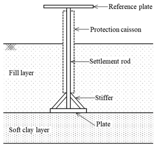
Figure 6.
Schematic of the settlement plate used in the study site.
A total of 50 settlement plates were installed at the site, with 15 positioned within the study area. Settlement measurements were conducted at these plates using a total station from January 2020 to March 2022, at intervals of 1 to 3 days. Each settlement plate in the study area covered approximately 10,400 m2, which highlights the relatively sparse instrumentation used over a large construction area. The daily measurements revealed a striking contrast in data volume, with the settlement plates providing 50 data points compared with the UAV LiDAR, which captured approximately 100 million data points.
3. Data Preprocessing
3.1. Denoising of the 3D Point Cloud
The effective preprocessing of 3D point cloud data, including denoising, interpolation, and bare-earth filtering, is essential for generating high-quality DEMs. Among these processes, denoising plays a critical role in enhancing surface data accuracy and ensuring the reliability of settlement analysis. Removing noise from the point cloud improves the clarity of surface representations, which leads to more accurate settlement calculations.
The LiDAR sensor used in this study operates on the time-of-flight principle, which generates approximately 300,000 points per second. Although these data provide high-resolution surface representation, noise in the point cloud can cause overlapping or distorted surface data due to laser reflection and refraction. If the noise remains unremoved, then noise can degrade the quality of 3D models or DEMs and significantly reduce the accuracy of precision analyses, such as settlement monitoring.
Various denoising techniques have been widely adopted to address the abovementioned challenges. Statistical outlier removal (SOR), moving least squares (MLS), and voxel grid (VG) are widely used methods for removing outliers [37,38,39]. The SOR method calculates the mean distance between a point and its neighbors to identify and remove outliers. The MLS method projects onto smooth and noise-free surface areas to improve data accuracy. The VG method divides the point cloud into 3D voxels and replaces each voxel with its centroid as a representative value [40].
This study evaluated the performance of SOR, MLS, and VG techniques for noise removal across three terrain types. These terrain types include construction materials, sloped terrain, and flat ground. Point cloud data were processed using CloudCompare v2.12 and QGIS v3.16 to compare the effectiveness of each denoising method under varying surface conditions.
Figure 7 presents three terrain types where denoising was performed using the SOR method. Figure 7a illustrates the aerial view of the study area, which highlights the location of the terrains. Figure 7b,c displays the corresponding point cloud representations before and after denoising, which allows for a comparative analysis of the effectiveness of the proposed method. Noise points removed by the SOR filter are highlighted in red, while the remaining ground points are shown in green. The results demonstrate the effectiveness of the method in reducing noise, while preserving key surface features.
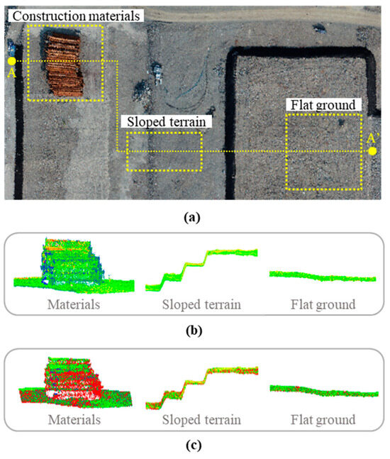
Figure 7.
Denoising of point cloud data in three terrain types: (a) three terrain types; (b) original point cloud data in section A-A’; (c) denoised point cloud data in section A-A’ by SOR.
For construction materials, the raw point cloud contains noise, which makes the 3D point cloud data unclear. After denoising, the data become more refined and show a well-defined stacked structure. In the sloped terrain, the pre-denoising point cloud presents outliers that distort the stepped elevation. The SOR method effectively removes these outliers, which preserves the natural terrain features. For flat ground, noise causes slight irregularities in the raw data. After denoising, the surface becomes smoother and more accurate.
To quantitatively assess the performance of the denoising techniques, the results were compared with ground truth data, as shown in Table 1. The evaluation considered three key metrics: the root mean square error (RMSE), the mean distance error (D) between points, and the mean angular error (θ) of normal vectors. These metrics provided insight into the accuracy of the noise removal process and its impact on surface representation.

Table 1.
RMSE, mean distance (D), and angular (θ) errors according to denoising methods and terrain types.
The analysis revealed several key findings from the noise removal results. Considering all terrain types collectively, the average RMSEs were 4.9 cm for both MLS and VG, and 5.1 cm for SOR. For the mean distance error, all methods produced errors ranging from 2 cm to 8 cm. The median error was approximately 1 cm, which demonstrated strong overall performance. The SOR method showed the best performance in terms of accuracy and processing efficiency when evaluating the mean angular error. The MLS method produced relatively higher errors on slopes. The VG method achieved similar accuracy to SOR but required more time due to voxelization. Based on these findings, the study identified the SOR method as the most effective technique for noise removal in terms of accuracy and computational efficiency.
3.2. Interpolation for the Optimal Grid Size
Interpolation involves converting irregularly distributed point cloud data into a uniform grid format to generate a DEM. This process is essential for accurate surface modeling. Smaller grid sizes have the advantage of capturing detailed surface features with high precision. However, smaller grids require more computation and are more susceptible to noise. On the contrary, larger grid sizes improve computational efficiency but risk losing detailed surface information. Therefore, determining the optimal grid size requires balancing precision and computational efficiency.
In this study, a flat ground surface and a settlement plate were used to determine the optimal grid size, as shown in Figure 8a,b. The flat ground surface was analyzed by incrementally increasing the grid size from 10 cm to 90 cm at 10 cm intervals. DEMs generated using the mean values at each grid size were compared with reference GPS survey data to evaluate their accuracy.
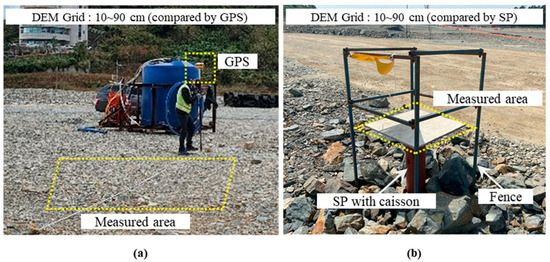
Figure 8.
Ground surface and settlement plate utilized for selecting optimal grid size: (a) ground surface; (b) settlement plate (SP).
For the settlement plate, the mean of the point cloud from the top-mounted reference plate was compared with the true instrumentation data. The side length of the reference plate was set to 50 cm. This length was chosen, given that it represents the protective barrier width area with the highest point density, which minimizes outlier influence on the mean. Smaller plates failed to achieve sufficient point density, which reduced reliability. Meanwhile, larger plates exceeded the dimensions of protective barriers, which introduced practical constraints. For the analysis of the optimal grid size, grid sizes were increased in 10 cm increments from 10 cm to 90 cm.
Table 2 illustrates the coefficient of determination (R2) of interpolation results on the ground surface and settlement plate in accordance with the grid size. The interpolation analysis showed high accuracy for grid sizes between 10 cm and 50 cm with the average R2 of 0.847 and 0.951. However, grid sizes larger than 60 cm exhibited increasing errors. This trend highlights the limitations of larger grid sizes in adequately reflecting detailed surface features. Subsequently, the rasterization of point cloud data was analyzed to determine the optimal grid size for generating DEMs. The analysis revealed that a grid size of 50 cm × 50 cm resulted in the highest accuracy with a maximum R2 of 0.870 and 0.967. Based on these results, this study determined the optimal grid size to be 50 cm × 50 cm, effectively balancing accuracy and feasibility for surface data and reference plate-based analyses.
Table 2.
Coefficient of determination (R2) of interpolation results on ground surface and settlement plate.
Given the LiDAR point density of tens of points per square meter, a 50 cm × 50 cm cell consistently contained multiple measurements, enabling robust averaging and noise reduction. Grids finer than 50 cm were overly sensitive to outliers and lacked sufficient point coverage; whereas, grids coarser than 50 cm began to smooth out critical localized settlement patterns. This analysis confirmed that 50 cm × 50 cm achieves the best trade-off among spatial detail, noise stability, and computational efficiency. By selecting a data-driven grid size optimization, we provide a novel methodological contribution and ensure robust, high-resolution spatial settlement analysis.
3.3. Bare-Earth Filtering for the DEM
Bare-earth filtering involves separating ground surface points from non-ground points to extract only ground surface data. Construction sites usually contain various obstacles, such as construction materials, vehicles, and workers on the ground surface. If these objects are ineffectively removed, then the quality of the DEM may be degraded. These elements can distort or obscure ground surface data, which reduces the accuracy of analysis. Therefore, bare-earth filtering is a crucial step in generating reliable DEMs.
A representative technique for bare-earth filtering is cloth simulation filtering (CSF). This method simulates draping a virtual cloth over the ground surface to extract ground surface points [41]. By adjusting various parameters that reflect the flexibility of the cloth and the characteristics of the data, the CSF technique can achieve high accuracy even in complex environments, such as construction sites.
This study utilized UAV LiDAR data acquired on 10 November 2021, to evaluate and optimize the parameters for bare-earth filtering, while data from the entire 10-month period were filtered using the established parameters. The CSF technique was used as the filtering method, and key parameters were optimized to enhance filtering accuracy. The rigidness parameter was set to two, and Slopesmooth was enabled to accommodate the site’s surcharge fill, which reached ten meters in height. A time-step of 0.65 was applied, and 500 iterations were run. An independent ground truth was established by manually classifying points in the construction material area as ground or non-ground. The primary parameters in the CSF method are threshold (hcc) and grid resolution (GR), which need to be adjusted depending on the data characteristics and terrain conditions.
hcc was varied from 0.01 to 0.3 in increments of 0.05 to ensure a diverse range of parameter combinations and derive optimal performance, while GR was varied from 0.1 to 3.5 in increments of 0.5. A total of 56 parameter combinations were applied for analysis. The parameter range was determined based on the terrain characteristics of the study site. Notably, the site included surcharge fill with a height of up to 10 m, which required the consideration of complex terrain conditions when setting the parameter range.
The filtering results were quantitatively evaluated using Cohen’s Kappa coefficient (k). Cohen’s Kappa coefficient quantifies the agreement between our LiDAR-based ground classification and an independent ground truth dataset, correcting for chance agreement. It is computed as shown in Equation (1).
where Po is the observed proportion of matching ground/non-ground labels, and Pe is the expected agreement by random assignment. This coefficient is an indicator of filtering accuracy, where k > 0.8 is generally considered to represent high accuracy [42]. The filtering performance of each parameter combination was compared using the Kappa coefficient, and the combination with the highest accuracy was selected as the optimal parameter setting.
k = (Po − Pe)/(1 − Pe),
Figure 9 presents the results of bare-earth filtering applied to construction materials. The bare-earth filtering results using the CSF technique showed significant variation depending on the parameter combinations. The Kappa coefficient ranged from a minimum of 0.1 to a maximum of 0.9, which highlights the critical impact of parameter settings on filtering accuracy. The parameter combination that achieved the highest accuracy resulted in a Kappa coefficient of k = 0.9.
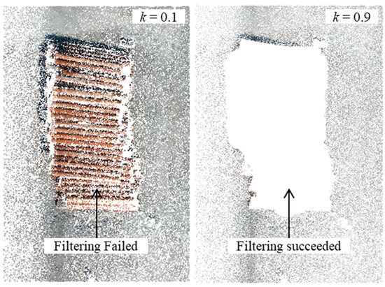
Figure 9.
Bare-earth filtering results applied to construction materials according to CSF parameters.
The achieved Kappa coefficient of 0.9 indicates almost perfect agreement with the independent ground truth, while visual inspection from Figure 9 confirmed that all above ground objects including construction materials were removed, and the true ground surface was preserved. These combined quantitative and qualitative validations confirm the robustness of our bare-earth filter and the high quality of the resulting DEMs used for subsequent settlement analyses.
Conversely, the combination with the lowest accuracy yielded a Kappa coefficient of k = 0.1. This result indicates that the separation between ground and non-ground points was inadequate, and some construction materials remained in the data. Based on these findings, this study applied the parameter combination with the highest accuracy to generate the DEM. This approach ensured the reliability of the filtering results and guaranteed the accuracy of subsequent analyses.
Figure 10 illustrates the monthly DEMs obtained from 26 May to 24 March through preprocessing UAV LiDAR data. In general, settlement can be evaluated by calculating the difference of DEMs (DoDs). This difference calculation reveals changes in elevation over time, which allows for the analysis of consolidation settlement.
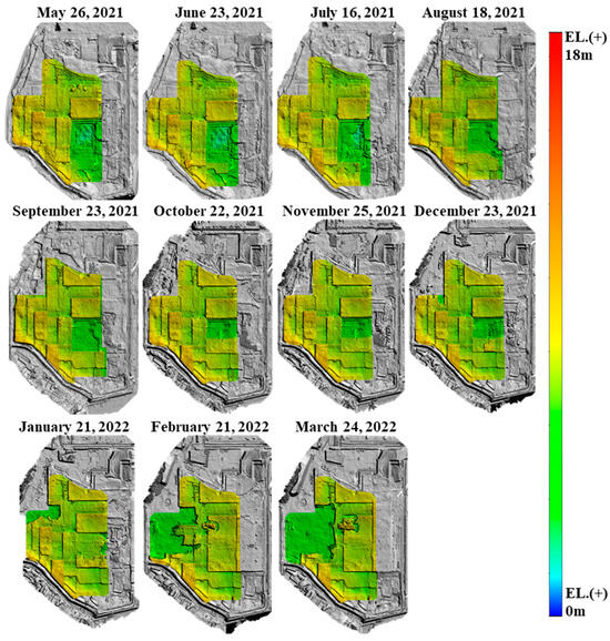
Figure 10.
Preprocessed monthly DEMs obtained by UAV LiDAR.
However, this approach can lead to significant errors in cases where staged loading (i.e., surcharge fill construction) occurs between measurements. Given that UAV LiDAR captures surface elevation, any surcharge fill construction data that occur between two measurement locations may cause the DoD calculations to show unreasonably large positive values (i.e., large heaving), which do not represent the true settlement.
Moreover, considering that large settlement occurs immediately following a load increase, accurately assessing this early-stage settlement is crucial to fully understand the soil behavior and consolidation progress. Therefore, this study introduces a simple settlement monitoring method designed to evaluate settlement even when staged loading events occur between UAV LiDAR measurements.
4. UAV LiDAR-Based Settlement Monitoring
4.1. Proposed Settlement Evaluation Method
Figure 11 illustrates the procedure for correcting timeseries settlement data during staged loading. The correction process accounts for periods where direct settlement measurements are impossible due to changes in ground elevation caused by fill operations. During resting periods when no additional fill is placed, such as between t1 and t2, settlement (s1 and s2) can be accurately evaluated using DoDs.
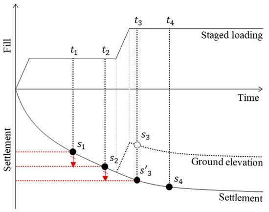
Figure 11.
Procedure of timeseries settlement data correction during staged loading.
However, during active filling periods, such as t2 to t3, accurate settlement estimation becomes challenging, because the observed change in ground elevation (s3) reflects actual settlement and the added fill thickness. As a result, using raw elevation data alone would lead to an overestimation of the surface level, making it impossible to isolate true settlement.
To address this issue, an interpolation method was applied, using settlement data from earlier stages (t1 to t2) to estimate settlement during the filling period (t2 to t3). This method offers several advantages. In soft ground, consolidation settlement generally decreases over time, meaning that directly applying earlier settlement trends could lead to overestimation. However, in staged preloading, rapid fill placement usually exceeds 1 m within a short period, which is typically less than a month. This sudden loading induces significant immediate settlement, which counterbalances the potential overestimation caused by using earlier data for interpolation.
By incorporating both the declining settlement trend over time and the increased settlement due to filling operations, this approach ensures a balanced and reliable estimation of cumulative settlement (s1-s2-s’3-s4). The correction method enhances the accuracy of timeseries settlement monitoring by effectively accounting for natural consolidation behavior and fill-induced settlement effects.
4.2. Settlement Evaluation and Analysis Using Proposed Method
Figure 12 shows the comparison of cumulative settlement range evaluated using UAV LiDAR and the proposed method over a 10-month period at four locations equipped with settlement plates. The cumulative settlement was calculated using the method from Figure 11, which was based on DoDs generated with a 0.5 m grid. The settlement distribution range, which was derived from UAV LiDAR measurements, is represented for the following three different sections centered on the settlement plate: 10 m × 10 m, 50 m × 50 m, and 100 m × 100 m.
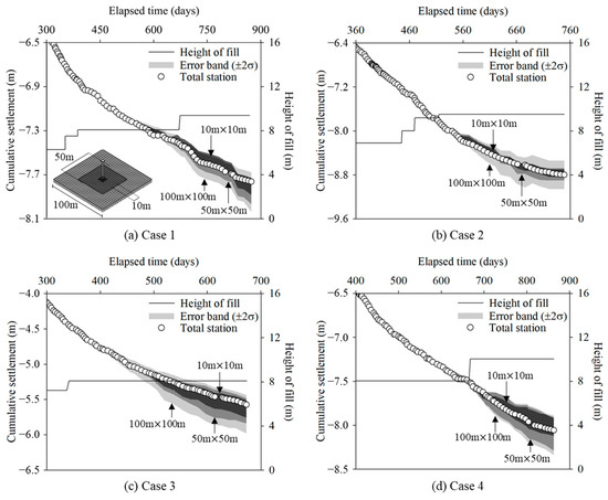
Figure 12.
Comparison of cumulative settlement range according to section size: (a) Case 1; (b) Case 2; (c) Case 3; (d) Case 4.
This study employed a confidence interval approach under the assumption of a normal distribution to ensure the reliability of UAV LiDAR-based settlement measurements and effectively account for measurement variability. In geotechnical engineering, the 95% confidence interval is widely used as a standard criterion for quantifying the variability of soil parameters and enhancing the reliability of analytical results based on statistical principles [43,44,45,46]. Accordingly, the reliability of the cumulative settlement distribution in this study was assessed based on a ±2 standard deviation range, which corresponds to an approximate 95% confidence interval.
Across all four cases (Figure 12), the settlement distribution ranges for the 10 m × 10 m and 50 m × 50 m sections generally align with total station measurements. However, the 100 m × 100 m sections show significantly broader distribution ranges, which highlights increased variability over larger areas. This consistent pattern indicates that, while UAV LiDAR effectively captures cumulative settlement trends, larger analysis areas introduce more variability, which should be considered in practical applications.
Figure 13 illustrates the comparison of cumulative settlement distribution across various section sizes, represented as normal distribution curves. For all cases, the average settlement values obtained from UAV LiDAR measurements for each section size of 10 m × 10 m align closely with those from the settlement plate measurements (TS). This close alignment indicates consistency in mean settlement across scales. However, the figures show that the deviation in the settlement distribution increases with larger section sizes.
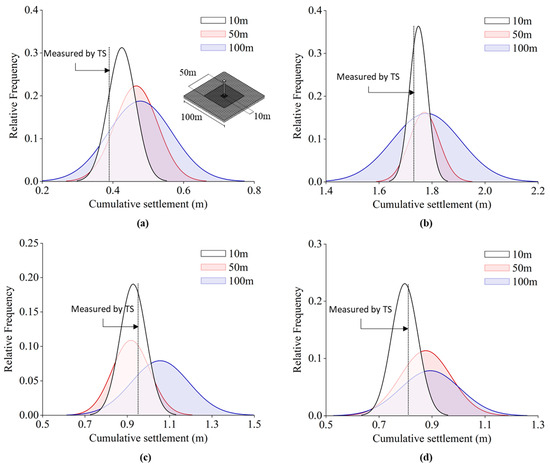
Figure 13.
Comparison of cumulative settlement distribution according to section size: (a) Case 1; (b) Case 2; (c) Case 3; (d) Case 4.
Notably, the 50 m × 50 m section displays a wider distribution than the 10 m × 10 m section, which reflects greater variability in settlement. By contrast, the distribution deviation between the 50 m × 50 m and 100 m × 100 m sections is comparable, which suggests an increase in deviation plateaus at larger scales. These results suggest that, while the average settlement remains stable, the variability of settlement distribution grows with section size, particularly when increasing from smaller to intermediate scales.
The results highlight the effectiveness of UAV LiDAR in delivering a precise spatial distribution of settlement that cannot be achieved by traditional methods using total stations. The differences in settlement observed across various section sizes reveal the impact of spatial variability in ground conditions. The increase in deviation with section size suggests that larger areas capture more localized variations in settlement behavior, which is potentially due to variations in soil properties or loading conditions.
4.3. Settlement Prediction and Analysis
This study utilized the proposed method and data from UAV LiDAR measurements to conduct settlement predictions and analyses. The hyperbolic method, which was proposed by Tan et al. [47], was employed for settlement forecasting. This approach is widely used for predicting future settlement based on post-preloading settlement observations, with the assumption that the settlement rate decreases hyperbolically over time. The time–settlement relationship is determined using field-measured settlement data following preloading.
Figure 14 presents the prediction of settlement based on the hyperbolic method. The coefficients α and β are determined by analyzing the relationship between (t − ti) and (t − ti)/(S − Si). In this study, we extended the hyperbolic method from its traditional application on single settlement gauges to a spatial framework by treating each 50 cm × 50 cm DEM grid cell as a virtual settlement gauge. Elevation changes recorded at each cell over successive UAV LiDAR surveys were assumed to follow a hyperbolic consolidation trend. Assuming that primary consolidation in soft clays produces a time–settlement response that follows a hyperbolic trend, we fitted a hyperbolic function to each cell’s time–settlement series and thereby extrapolated its final settlement. This approach utilized data from seven bi-weekly surveys conducted under relatively constant surcharge loading, conditions under which the hyperbolic method has proven reliable in field practice [13,47]. By applying hyperbolic extrapolation to DEM-derived spatial datasets, we achieve a novel integration of classical consolidation theory with high-resolution spatial monitoring.
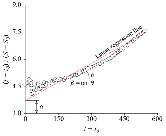
Figure 14.
Prediction of settlement based on the hyperbolic method.
Si and ti represent the settlement and time following the final fill, respectively. The coefficients are used in Equation (2) for forecasting settlement over time. In addition, the final settlement (Sf) can be calculated as demonstrated in Equation (3).
where St represents the predicted settlement at time t; Si represents the initial settlement; ti represents the initial time; and α and β represent the y-intercept and the slope of the regression line, respectively.
Figure 15 presents the settlement prediction results over time derived from the proposed method using UAV LiDAR measurements. Shaded area denotes the final−fill data period used for the hyperbolic prediction. The predictions are based on the average settlement within the following three section sizes: 10 m × 10 m, 50 m × 50 m, and 100 m × 100 m. These results are compared against predictions derived from settlement plate measurements using total station (TS) to evaluate the discrepancy between UAV LiDAR and settlement plate measurements.
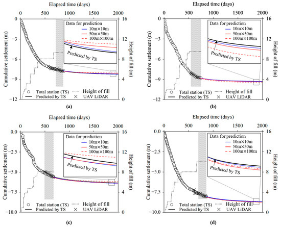
Figure 15.
Settlement predictions using the hyperbolic method according to section size: (a) Case 1; (b) Case 2; (c) Case 3; (d) Case 4.
Table 3 illustrates the discrepancy of predicted final settlement between UAV LiDAR and settlement plate measurements using the hyperbolic method (Equation (2)). Across all cases, the difference in predicted final settlement increases as the section size increases from 10 m × 10 m to 100 m × 100 m. For instance, the differences range from 0.01 to 0.36 for Case 1, 0.04 to 0.23 for Case 2, 0.01 to 0.44 for Case 3, and 0.05 to 0.06 for Case 4. This consistent trend highlights the impact of spatial variability on settlement predictions, which emphasizes the importance of considering section size when evaluating settlement data.
Table 3.
Final settlement prediction discrepancy between UAV LiDAR and settlement plate measurements according to section size.
For all cases, predictions based on the 10 m × 10 m section yielded an average discrepancy of 0.03 m. In contrast, when the section size increased to 50 m × 50 m, the prediction discrepancy increased by 5 times. For the 100 m × 100 m section, the discrepancy was on 10 times greater than that of the 10 m × 10 m section.
For all cases, the predictions based on the 10 m × 10 m section show the smallest discrepancy compared with the predictions based on the settlement plate measurements. The discrepancy increased as the section size rose to 50 m × 50 m and 100 m × 100 m. This trend aligns with the findings in Figure 12 and Figure 13, where variations in settlement across different section sizes were observed. The increase in the difference is primarily due to the spatial variability of the settlement, where larger sections tend to average out localized settlement variations, leading to discrepancies in prediction accuracy. These results indicate that, while settlement plates provide highly representative measurements at a local scale (approximately 10 m), their representativeness diminishes at larger scales due to increased spatial variability in settlement.
In addition to the spatial section analysis, the influence of UAV LiDAR measurement frequency on final settlement prediction accuracy was examined following the completion of surcharge fill construction. UAV LiDAR surveys were conducted at 2-week intervals, and predictions were generated based on four, five, six, and seven measurements using the 10 m × 10 m section. These predictions were then compared with the settlement plate results.
Figure 16 and Table 4 present the settlement prediction results according to the measurement frequency. Shaded area indicates the final−fill period used for the hyperbolic prediction, covering the 4−7 UAV LiDAR measurements taken at 2−week intervals. The results showed that increasing the measurement frequency led to enhanced prediction accuracy. With four and five surveys, the average prediction discrepancies were 0.23 m and 0.13 m, respectively. When six surveys were utilized, the average discrepancy decreased to 0.12 m. Predictions based on seven surveys exhibited final discrepancies ranging from 0.02 m to 0.08 m, all of which were less than 0.1 m. These findings suggest that a limited measurement frequency may fail to capture the initial settlement rate and subsequent consolidation settlement behavior accurately. This failure leads to the underestimation of the final settlement. On the contrary, a measurement frequency of at least seven surveys, which were conducted at 2-week intervals, provides sufficient data to reliably reflect the early-stage settlement rate and achieve high prediction accuracy.
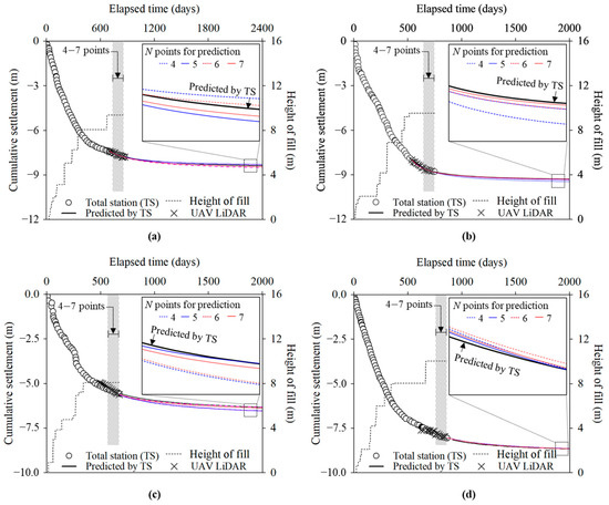
Figure 16.
Settlement predictions using the hyperbolic method according to measurement frequency: (a) Case 1; (b) Case 2; (c) Case 3; (d) Case 4.
Table 4.
Final settlement prediction discrepancy between UAV LiDAR and settlement plate measurements according to measurement frequency.
Collectively, these results demonstrate that settlement plates maintain high spatial representativeness at a fine section resolution (approximately 10 m), but UAV LiDAR data capture increased the variability at coarser section scales. This comparative analysis underscores the importance of selecting an appropriate section size and measurement frequency to balance spatial detail and prediction accuracy in settlement monitoring.
5. Conclusions
This study presented a comprehensive methodology for UAV LiDAR-based spatial representativeness analysis in soft ground settlement prediction. Its utility was validated through comparisons with conventional ground-based monitoring systems using settlement plates. The research database was constructed from UAV LiDAR measurements conducted at 2-week intervals at Busan Newport between May 2021 and March 2022. The contributions of this study can be summarized as follows:
- (1)
- A robust data preprocessing framework was developed by integrating advanced techniques. Specifically, the SOR method was applied for denoising, the optimal grid size was determined through interpolation analysis, and the CSF method was employed for effective bare-earth extraction. Therefore, these processes resulted in high-quality DEMs that significantly enhance data accuracy and computational efficiency.
- (2)
- A novel settlement evaluation method was proposed to overcome challenges associated with staged loading. By incorporating timeseries corrections and interpolation techniques, this approach accurately captures surcharge fill and consolidation settlement. An evaluation of cumulative settlement over various section sizes (10 m × 10 m, 50 m × 50 m, and 100 m × 100 m) demonstrated that, while average settlement values remain stable at finer scales, spatial variability increases with larger section sizes.
- (3)
- Comparative analysis revealed that settlement plates exhibit excellent spatial representativeness within a local area of approximately 10 m × 10 m. In contrast, larger section sizes resulted in significantly higher prediction discrepancies due to increased spatial variability. Furthermore, the findings confirm that a minimum of seven UAV LiDAR surveys at 2-week intervals is essential for reliably capturing early-stage settlement behaviors. This discovery provides clear guidelines for measurement frequency in geotechnical monitoring.
- (4)
- The methodology was both developed for and validated in a marine environment and is directly transferable to similar coastal infrastructure projects worldwide. For example, it can be applied to monitor settlement in newly reclaimed port and airport sites, to safeguard the stability of embankments and breakwaters founded on soft seabed deposits, and to optimize ground improvement schedules. Furthermore, the demonstrated requirement for at least seven UAV LiDAR surveys to capture early-stage settlement, together with our analysis of spatial variability, provides essential guidance for formulating monitoring strategies in large-scale marine projects operating under strict construction timelines. By enabling the early detection of differential settlement beneath structures on reclaimed land and facilitating prompt reinforcement measures, this framework can help prevent costly structural failures.
In summary, the UAV LiDAR-based framework for consolidation settlement monitoring developed in this study enables highly accurate settlement prediction and detailed spatial variability assessment in deep soft ground. Furthermore, this framework provides practical guidelines for optimal data preprocessing, section size selection, and measurement frequency. These contributions are expected to significantly advance geotechnical monitoring and settlement management practices.
Author Contributions
Conceptualization, S.-J.K. and S.H.; data curation, S.-J.K. and S.H.; formal analysis, S.-J.K. and S.H.; funding acquisition, T.-Y.K.; investigation, T.-Y.K.; methodology, T.-Y.K.; project administration, T.-Y.K.; resources, T.-Y.K.; software, S.-J.K.; supervision, S.H. and T.-Y.K.; validation, S.H. and T.-Y.K.; visualization, S.-J.K.; writing—original draft, S.-J.K.; writing—review and editing, S.H. and T.-Y.K. All authors have read and agreed to the published version of the manuscript.
Funding
Research for this paper was carried out under the KICT Research Program (project no. 20250270-001, Intelligent Geotechnical Data Analysis and Underground Infrastructure Stability Assessment Based on Data Fusion) funded by the Ministry of Science and ICT.
Data Availability Statement
The original contributions presented in this study are included in the article. Further inquiries can be directed to the corresponding authors.
Conflicts of Interest
Author Seok-Jun Ko was employed by the company GS E&C. The remaining authors declare that the research was conducted in the absence of any commercial or financial relationships that could be construed as a potential conflict of interest.
Abbreviations
The following abbreviations are used in this manuscript:
| Digital elevation model | DEM |
| Deep cement mixing | DCM |
| Unconfined compressive strength test | UCS |
| Standard penetration test | SPT |
| Flat dilatometer test | DMT |
| Real-time kinematic | RTK |
| Ground control point | GCP |
| Korean National Geoid Model 2018 | KNGeoid18 |
| Time-of-flight | TOF |
| Statistical outlier removal | SOR |
| Moving least squares | MLS |
| Voxel grid | VG |
| Mean distance error | D |
| Mean angular error | Θ |
| Coefficient of determination | R2 |
| Cloth simulation filtering | CSF |
| Threshold | hcc |
| Grid resolution | GR |
| Cohen’s Kappa coefficient | k |
| Difference of digital elevation models | DoDs |
| Total station | TS |
| Final settlement | Sf |
References
- An, S.; Yuan, L.; Xu, Y.; Wang, X.; Zhou, D. Ground subsidence monitoring based on UAV-LiDAR technology: A case study of a mine in the Ordos, China. Geomech. Geophys. Geo-Energy Geo-Resour. 2024, 10, 57. [Google Scholar] [CrossRef]
- Ćwiąkała, P.; Gruszczyński, W.; Stoch, T.; Puniach, E.; Mrocheń, D.; Matwij, W.; Wójcik, A. UAV applications for determination of land deformations caused by underground mining. Remote Sens. 2020, 12, 1733. [Google Scholar] [CrossRef]
- Barron, R.A. Consolidation of fine-grained soils by drain wells. Trans. Am. Soc. Civ. Eng. 1948, 113, 718–742. [Google Scholar] [CrossRef]
- Christian, J.T.; Carrier, W.D., III. Janbu, Bjerrum and Kjaernsli’s chart reinterpreted. Can. Geotech. J. 1978, 15, 123–128. [Google Scholar] [CrossRef]
- De Wet, J.A. Three-dimensional consolidation. Highw. Res. Board Bull. 1962, 342, 152–175. [Google Scholar]
- Janbu, N. Consolidation of clay layers based on non-linear stress-strain. In Proceedings of the Sixth International Conference on Soil Mechanics and Foundation Engineering, Montreal, QC, Canada, 8–15 September 1965; Volume 2, pp. 83–87. [Google Scholar]
- Pyrah, I.C. One-dimensional consolidation of layered soils. Geotechnique 1996, 46, 555–560. [Google Scholar] [CrossRef]
- Terzaghi, K. Theoretical Soil Mechanics; John Wiley & Sons: New York, NY, USA, 1943. [Google Scholar]
- Yin, J.H.; Chen, Z.J.; Feng, W.Q. A general simple method for calculating consolidation settlements of layered clayey soils with vertical drains under staged loadings. Acta Geotech. 2022, 17, 3647–3674. [Google Scholar] [CrossRef]
- Zhou, W.H.; Zhao, L.S.; Lok, T.M.H.; Mei, G.X.; Li, X.B. Analytical solutions to the axisymmetrical consolidation of unsaturated soils. J. Eng. Mech. 2018, 144, 04017152. [Google Scholar] [CrossRef]
- Jiang, X.; Chen, X.; Fu, Y.; Gu, H.; Hu, J.; Qiu, X.; Qiu, Y. Analysis of settlement behaviour of soft ground under wide embankment. Balt. J. Road Bridge Eng. 2021, 16, 153–175. [Google Scholar] [CrossRef]
- Tashiro, M.; Noda, T.; Inagaki, M.; Nakano, M.; Asaoka, A. Prediction of settlement in natural deposited clay ground with risk of large residual settlement due to embankment loading. Soils Found. 2011, 51, 133–149. [Google Scholar] [CrossRef][Green Version]
- Sridharan, A.; Murthy, N.S.; Prakash, K. Rectangular hyperbola method of consolidation analysis. Geotechnique 1987, 37, 355–368. [Google Scholar] [CrossRef]
- Tan, T.S.; Inoue, T.; Lee, S.L. Hyperbolic method for consolidation analysis. J. Geotech. Eng. 1991, 117, 1723–1737. [Google Scholar] [CrossRef]
- Asaoka, A. Observational procedure of settlement prediction. Soils Found. 1978, 18, 87–101. [Google Scholar] [CrossRef]
- Kwak, T.Y.; Hong, S.; Lee, J.H.; Woo, S.I. Analysis of the limitations of the existing subsidence prediction method based on the subsidence measurement data and suggestions for improvement method through weighted non-linear regression analysis. J. Korean Geotech. Soc. 2022, 38, 103–112. (In Korean) [Google Scholar]
- Kwak, T.Y.; Woo, S.I.; Hong, S.; Lee, J.H.; Baek, S.H. Settlement prediction accuracy analysis of weighted nonlinear regression hyperbolic method according to the weighting method. J. Korean Geotech. Soc. 2023, 38, 103–112. (In Korean) [Google Scholar]
- Hong, S.; Lee, M.H.; Yoo, B.S.; Kwak, T.Y.; Kim, S.R. Application of deep learning algorithms for predicting consolidation settlement. KSCE J. Civ. Eng. 2025, 29, 100072. [Google Scholar] [CrossRef]
- Hong, S.; Ko, S.J.; Woo, S.I.; Kwak, T.Y.; Kim, S.R. Time-series forecasting of consolidation settlement using LSTM network. Appl. Intell. 2024, 54, 1386–1404. [Google Scholar] [CrossRef]
- Tan, S.; Chew, S. Comparison of the hyperbolic and Asaoka observational method of monitoring consolidation with vertical drains. Soils Found. 1996, 36, 31–42. [Google Scholar] [CrossRef] [PubMed]
- Oladunjoye, O.; Fok, K.; Zaremba, G.; Smith, V.; Clayton, G. LiDAR and multispectral sensing for monitoring SMPs: A review of current applications and future opportunities. J. Sustain. Water Built Environ. 2025, 11, 04025001. [Google Scholar] [CrossRef]
- Vishweshwaran, M.; Sujatha, E.R. A review on applications of drones in geotechnical engineering. Indian Geotech. J. 2024, 55, 2091–2105. [Google Scholar] [CrossRef]
- Sankey, T.; Donager, J.; McVay, J.; Sankey, J.B. UAV lidar and hyperspectral fusion for forest monitoring in the southwestern USA. Remote Sens. Environ. 2017, 195, 30–43. [Google Scholar] [CrossRef]
- Chase, A.F.; Chase, D.Z.; Fisher, C.T.; Leisz, S.J.; Weishampel, J.F. Geospatial revolution and remote sensing LiDAR in Mesoamerican archaeology. Proc. Natl. Acad. Sci. USA 2012, 109, 12916–12921. [Google Scholar] [CrossRef] [PubMed]
- Giordan, D.; Hayakawa, Y.; Nex, F.; Remondino, F.; Tarolli, P. The use of remotely piloted aircraft systems (RPASs) for natural hazards monitoring and management. Nat. Hazards Earth Syst. Sci. 2018, 18, 1079–1096. [Google Scholar] [CrossRef]
- Adade, R.; Aibinu, A.M.; Ekumah, B.; Asaana, J. Unmanned aerial vehicle (UAV) applications in coastal zone management—A review. Environ. Monit. Assess. 2021, 193, 1–12. [Google Scholar] [CrossRef]
- Curcio, A.C.; Peralta, G.; Aranda, M.; Barbero, L. Evaluating the performance of high spatial resolution UAV-photogrammetry and UAV-LiDAR for salt marshes: The Cádiz Bay study case. Remote Sens. 2022, 14, 3582. [Google Scholar] [CrossRef]
- Kim, J.; Hong, I. Evaluation of the usability of UAV LiDAR for analysis of karst (doline) terrain morphology. Sensors 2024, 24, 7062. [Google Scholar] [CrossRef]
- Lin, Y.C.; Cheng, Y.T.; Zhou, T.; Ravi, R.; Hasheminasab, S.M.; Flatt, J.E.; Habib, A. Evaluation of UAV LiDAR for mapping coastal environments. Remote Sens. 2019, 11, 2893. [Google Scholar] [CrossRef]
- Sofonia, J.; Phinn, S.; Roelfsema, C.; Kendoul, F. Observing geomorphological change on an evolving coastal sand dune using SLAM-based UAV LiDAR. Remote Sens. Earth Syst. Sci. 2019, 2, 273–291. [Google Scholar] [CrossRef]
- Bi, R.; Gan, S.; Yuan, X.; Li, R.; Gao, S.; Yang, M.; Hu, L. Multi-view analysis of high-resolution geomorphic features in complex mountains based on UAV-LiDAR and SfM-MVS: A case study of the northern pit rim structure of the Mountains of Lufeng, China. Appl. Sci. 2023, 13, 738. [Google Scholar] [CrossRef]
- Lee, J.; Jo, H.; Oh, J. Application of drone LiDAR survey for evaluation of a long-term consolidation settlement of large land reclamation. Appl. Sci. 2023, 13, 8277. [Google Scholar] [CrossRef]
- Xing, X.; Zhu, L.; Liu, B.; Peng, W.; Zhang, R.; Ma, X. Measuring land surface deformation over soft clay area based on an FIPR SAR interferometry algorithm—A case study of Beijing Capital International Airport (China). Remote Sens. 2022, 14, 4253. [Google Scholar] [CrossRef]
- Zhang, X.; Bao, Y.; Wang, D.; Xin, X.; Ding, L.; Xu, D.; Shen, J. Using UAV LiDAR to extract vegetation parameters of Inner Mongolian grassland. Remote Sens. 2021, 13, 656. [Google Scholar] [CrossRef]
- Wang, G.; Zhang, X.; Liu, X.; Wang, H.; Xu, L.; Liu, H.; Peng, L. Soil arching effect in reinforced piled embankment for motor-racing circuit: Field tests and numerical analysis. Transp. Geotech. 2022, 37, 100844. [Google Scholar] [CrossRef]
- Wang, G.; Zhang, X.; Liu, X.; Chang, Z.; Liu, Z.; Li, Y. Development of a neutral plane in PHC-supported embankments over soft soils: A case study of a motor-racing circuit. Int. J. Geomech. 2024, 24, 05023013. [Google Scholar] [CrossRef]
- Carrilho, A.C.; Galo, M.; Santos, R.C. Statistical outlier detection method for airborne LiDAR data. Int. Arch. Photogramm. Remote Sens. Spatial Inf. Sci. 2018, 42, 87–92. [Google Scholar] [CrossRef]
- Kang, C.L.; Lu, T.N.; Zong, M.M.; Wang, F.; Cheng, Y. Point cloud smooth sampling and surface reconstruction based on moving least squares. Int. Arch. Photogramm. Remote Sens. Spatial Inf. Sci. 2020, 42, 145–151. [Google Scholar]
- Rusu, R.B.; Cousins, S. 3D is here: Point cloud library (PCL). In Proceedings of the IEEE International Conference on Robotics and Automation, Shanghai, China, 9–13 May 2011; pp. 1–4. [Google Scholar]
- Hu, J.S.; Kuai, T.; Waslander, S.L. Point density-aware voxels for LiDAR 3D object detection. In Proceedings of the IEEE/CVF Conference on Computer Vision and Pattern Recognition, New Orleans, LA, USA, 19–24 June 2022; pp. 8469–8478. [Google Scholar]
- Zhang, W.; Qi, J.; Wan, P.; Wang, H.; Xie, D.; Wang, X.; Yan, G. An easy-to-use airborne LiDAR data filtering method based on cloth simulation. Remote Sens. 2016, 8, 501. [Google Scholar] [CrossRef]
- Landis, J.R.; Koch, G.G. An application of hierarchical kappa-type statistics in the assessment of majority agreement among multiple observers. Biometrics 1977, 33, 363–374. [Google Scholar] [CrossRef]
- Fillion, M.H.; Hadjigeorgiou, J.; Grenon, M.; Caumartin, R. Practical considerations in establishing the statistical reliability of geomechanical data. Geotech. Geol. Eng. 2020, 38, 169–190. [Google Scholar] [CrossRef]
- Han, L.; Zhang, W.; Wang, L.; Fu, J.; Xu, L.; Wang, Y. A reliability analysis framework coupled with statistical uncertainty characterization for geotechnical engineering. Geosci. Front. 2024, 15, 101913. [Google Scholar] [CrossRef]
- Phoon, K.K.; Ching, J. Better correlations for geotechnical design. In A Decade of Geotechnical Advances 2008–2017; ASCE: Reston, VA, USA, 2017; pp. 73–102. [Google Scholar]
- Prästings, A.; Spross, J.; Larsson, S. Characteristic values of geotechnical parameters in Eurocode 7. Proc. Inst. Civ. Eng. Geotech. Eng. 2019, 172, 301–311. [Google Scholar] [CrossRef]
- Tan, S.A. Ultimate settlement by hyperbolic plot for clays with vertical drains. J. Geotech. Eng. 1993, 119, 950–956. [Google Scholar] [CrossRef]
Disclaimer/Publisher’s Note: The statements, opinions and data contained in all publications are solely those of the individual author(s) and contributor(s) and not of MDPI and/or the editor(s). MDPI and/or the editor(s) disclaim responsibility for any injury to people or property resulting from any ideas, methods, instructions or products referred to in the content. |
© 2025 by the authors. Licensee MDPI, Basel, Switzerland. This article is an open access article distributed under the terms and conditions of the Creative Commons Attribution (CC BY) license (https://creativecommons.org/licenses/by/4.0/).