Abstract
A passive time reversal method with a metamodel (PTR-MM) is proposed to improve underwater source localization under ocean conditions. PTR-MM eliminates model mismatch errors by replacing the conventional sound propagation model with a Kriging metamodel. This metamodel is optimally constructed based on measured sound field data. The method combines a metamodel with a passive time reversal (PTR) process to generate a focused sound field whose intensity peaks correspond to source positions. In numerical simulations using the KRAKEN model in a range-independent waveguide, PTR-MM accurately localizes single and multiple sources, is insensitive to mismatches in key environmental parameters, and maintains unbiased performance down to −20 dB signal-to-noise ratios (SNRs). Experimental validation on the SWellEx-96 Event S5 dataset confirms that PTR-MM outperforms conventional PTR in both single- and dual-source localizations, achieving most mean absolute percentage errors (MAPEs) below 10% when trained and tested in consistent environments. Further studies reveal that localization accuracy depends primarily on signal quality, array aperture, and element spacing, rather than on source frequency. However, PTR-MM performance degrades if the metamodel is trained in an environment that differs from the test conditions. The above findings demonstrate the potential of combining PTR with a metamodel for robust and real-time localization.
1. Introduction
Underwater source localization is used to detect various underwater targets, such as fish and submarines, making it a critical task in both civilian and military fields [1]. It has emerged as a research hotspot in applied ocean acoustics [2]. Common methods for underwater source localization include direction-of-arrival (DOA) approach, beamforming, the time-difference-of-arrival (TDOA) technique, matched field processing (MFP), and the phase conjugation (PC) or time reversal (TR) method [3,4]. In recent years, machine learning (ML) has introduced a new paradigm for underwater source localization [5].
The DOA approach locates sources by measuring the direction of arrival at multiple vector hydrophones, while TDOA is a time-domain source localization technique that estimates the source position by measuring the time differences at which the sound signal reaches different hydrophones [3]. In a complex ocean environment, both DOA and TDOA are highly affected by noise and multipath effects, which can significantly degrade localization accuracy [6,7,8]. Beamforming is a spatial filtering technique that processes the sound pressure signals recorded by an array, and it is widely used for sound source localization [2,3,9]. Numerous beamforming algorithms offer a variety of solutions for localizing sources in different environments, such as delay-and-sum [10], minimum-variance distortionless response (MVDR) [11], and multiple signal classification (MUSIC) [12]. Typically, beamforming is used to localize mid-to-high frequency sources. While localizing low-frequency sound sources, beamforming generally requires large-aperture arrays to achieve the necessary spatial resolution [4]. MFP, an extension of plane wave beamforming, is commonly used for source localization in complex but known multidimensional acoustic environments [13,14]. MFP has found applications in wind tunnels, structural vibration, and photoacoustics [3]. Compared to other localization techniques in known environments, MFP can achieve superior localization performance due to its ability to exploit environmental complexity [15]. However, MFP is known to suffer from model mismatch issues (i.e., differences between the actual acoustic field and the replica field) [16].
The PC or TR method is regarded as an active implementation of MFP, and PC in the frequency domain is equivalent to TR in the time domain [4]. Jackson and Dowling [17] introduced PC into underwater acoustics and detailed its fundamental theory. TR (or PC) operates by first reversing (or conjugating) the signals received by the source–receiver array in the time (or frequency) domain. These processed signals are then retransmitted as excitation signals through a transmitting array that is co-located with the receiving array. Depending on the TR field generation method, TR methods are divided into active time reversal (ATR) [18,19,20,21] or PTR [22,23,24,25,26,27]. ATR employs a physical vertical array to generate a TR pressure field between the detection source and the receiving array. In contrast, PTR simulates the TR pressure field using acoustic propagation models. ATR is primarily constrained by the unknown position of the detection source. PTR is limited by model mismatch [2]. ML is regarded as an optimization technique from a statistical perspective. ML-based methods localize sources by identifying patterns in pressure data. Compared to classical methods, ML-based methods are not limited by model mismatch [5]. Various ML methods have been applied to source localization, including support vector machines (SVMs) [28,29], feedforward neural networks (FNNs) [30], convolutional neural networks (CNNs) [31,32], generalized regression neural network (GRNNs) [33], and deep neural networks (DNNs) [34]. However, ML-based underwater source localization faces several challenges, such as localization in uncertain ocean environments, low SNR conditions, and simultaneous localization of multiple sources [5].
Metamodels are a data-driven modeling technique that centers on constructing a real-time analysis model to replace a high-accuracy physical model [35]. A metamodel is required to reduce computational cost while retaining high accuracy. Metamodel methods have been widely applied in acoustic areas such as vibro-acoustic radiation modeling [36], noise and vibration reduction design optimization [37,38], and ocean environment observatory or inversion [39,40]. Recently, metamodel methods have been also used to localize acoustic sources. Goupy [41] realized atmospheric source localization by combining Bayesian inversion with a polynomial chaos decomposition (PCE) metamodel. Chen and Li [42] proposed a dynamic weight meta-learning method (DWML) to localize an underwater source based on limited experimental data. Jenkins et al. [43] used a Bayesian optimization with a Gaussian process surrogate model to localize a source in a shallow-water waveguide. But all of the above metamodel-based source localization methods do not address the multi-source localization problem.
Given the high accuracy modeling capability of metamodels, this paper proposes a PTR-MM method by replacing the sound propagation model with a metamodel. In this method, the sound propagation metamodel is constructed using measured sound field signals and combined with a PTR process to localize underwater sound sources. By employing a data-driven metamodel instead of a physical propagation model, the method avoids the common model mismatch. Moreover, the multi-source localization capability of TR resolves the challenge of multiple-source localization in purely data-driven methods. The basic framework and theoretical foundation of PTR-MM are detailed in Section 2. Simulations in Section 3 and the experiment in Section 4.2 demonstrate the performance and noise robustness of PTR-MM. In Section 4.3, the effects of frequency and array parameters on PTR-MM are studied. The conclusions are summarized in Section 5.
2. Passive Time Reversal Method with Metamodel
2.1. The Framework of Passive Time Reversal Method with Metamodel
PTR-MM is mainly divided into two parts. The first part is constructing a sound propagation metamodel, and the second is generating a TR sound field. The source localization process using PTR-MM is shown in Figure 1. PTR-MM transforms the array sound signals into a TR sound field heat map with corresponding source position coordinates in real time, thus realizing the visualization and localization of single or multiple sound sources within the investigated area.
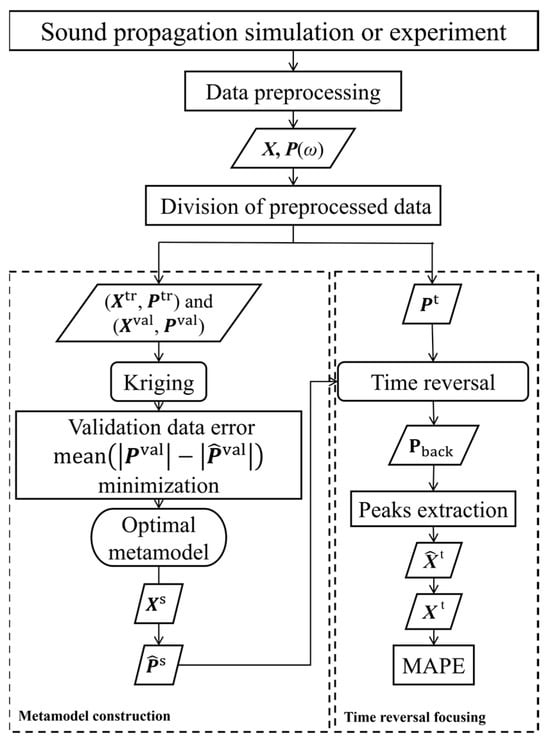
Figure 1.
Source localization process using PTR-MM.
The sound propagation simulation and experiment yield the source position and the time-domain sound pressure signals received by each array element. After data preprocessing, the source position and the frequency-domain sound pressure signals at the array are obtained, where denotes the angular frequency. The preprocessed data are divided into training , validation , and test sets . The training and validation sets are used to build the sound propagation metamodel, while the test set is employed to evaluate the localization performance of PTR-MM. The sound propagation metamodel is an optimal Kriging model designed to minimize the difference between the predicted and actual sound pressure amplitudes in the validation set. The discretized position coordinates of the potential source region are input to the sound propagation metamodel to obtain the sound pressures between the sound sources of the potential source region and each array element. The reverse-propagated sound field is obtained by TR using and . The location corresponding to the peak of serves as the predicted sources position of test set . The PTR-MM localization performance is quantified through the MAPE between and .
2.2. Data Preprocessing
Assume that the data obtained from sound propagation simulations or experiments consist of sound sources positions (where is the spatial dimensions and , is the set of real numbers) and the time-domain sound pressure signals are recorded by an array of hydrophones over time segments, (where and ). First, is segmented into segments based on the sound source positions, each of which is further divided into snapshots. Next, a discrete Fourier transform (DFT) is performed on the time-domain signals in each snapshot to convert it into frequency-domain sound pressure signals. Let the frequency-domain sound pressure data for the th sound source at the th snapshot be (where denotes frequency number, , and is the set of complex numbers). We assume that the frequency of is , and the angular frequency will be . Then the sound pressure at the th frequency can be expressed as
where and , is the noise, is the source intensity amplitude, is the Green’s function, and is the array position matrix. Next, the sound pressure is normalized to ensure that only the Green’s function between the sources and the array elements is used for localization
where and respectively represent the absolute value operator and Euclidean norm operator.
According to Equation (2), the sound pressures at frequencies are normalized, and the normalized frequency-domain sound pressure data for the th sound source at the th snapshot is . Finally, the sound pressure data between the th sound source and the array elements is defined as the average over snapshots
where is the snapshot number, and denotes the th snapshot.
Through DFT, normalization in Equation (2) and averaging in Equation (3), the time-domain sound pressure signals are transformed into the normalized frequency-domain sound pressure signals . The above signals are generated by sound sources and recorded in a vertical linear array (VLA) with hydrophones.
2.3. Division of Preprocessed Data
The sound source positions and the corresponding frequency-domain sound pressure data are divided into training , validation , and test sets . Importantly, the data in the training set must be distinct from those in the validation and test sets. The training set is used to train the sound propagation metamodel. The objective function for optimizing the metamodel parameters is which represents the Euclidean norm of the difference between the predicted and actual frequency-domain sound pressure amplitude for validation set. The localization performance of PTR-MM is quantified by MAPE between the predicted and the actual source positions of the test set
where is the number of sources in test set, and denotes the source, and .
2.4. Metamodel Construction
Given the widespread application of the Kriging model in vibration and acoustics, the sound propagation metamodel is still constructed by the Kriging method. Comparisons with alternative algorithms are beyond the scope of this study. The training set and validation set are used to train the metamodel. The inputs of the sound propagation metamodel are sound source positions, while outputs are the frequency-domain sound pressure data. If the training set contains sound sources, is a source positions matrix of dimensions and is a frequency-domain sound pressure matrix of dimensions . In this study, the Kriging metamodel is constructed by the UQLab toolbox [44], which performs independent modeling for each output variable in vector-valued (multi-output) models. However, the UQLab toolbox is limited to construct real-valued outputs models and does not support complex-valued outputs models. Therefore, metamodels are constructed for the real and imaginary part of , respectively, for each frequency, resulting in a total of metamodels whose inputs are final source positions.
For simplicity, the basic theory of the Kriging metamodel is briefly discussed by the real part of the complex sound pressure at the th frequency, and , where denotes the th source. The Kriging method models as a function of , and the general equation of the Kriging model is expressed as
where is an -dimension function set with trend functions, is an unknown coefficient set of the trend functions and , and is a Gaussian random process whose mean is 0 and whose covariance is expressed as
where and are different vectors of a source position matrix , is the variance of the Gaussian random process, and is the correlation function with an unknown parameter ; the correlation function is defined in Equation (9).
For the training set , , the predicted real part of the sound pressure at an arbitrary sound source position for the th frequency, and the th array element is given as follows using the real part of the complex sound pressure data at the same frequency and array element from , and .
where is an unknown coefficient vector prediction with dimensions , is an -dimension correlation function matrix between the source positions of training set, is a correlation function vector with dimensions of between and the training set source positions, and is an -dimension trend function matrix.
Since the sound propagation metamodel inherently accounts for all disturbances such as attenuation, dissipation, and noise, it is regarded as a “noiseless” regression model. For such noiseless models, the maximum likelihood estimation method can be employed to estimate the unknown parameters vector of the correlation functions and the process variance :
where is the determinant of . If the above model is used to simultaneously predict the real parts of the complex sound pressure recorded by array elements, expands to a matrix of dimensions , and becomes a vector of dimensions , and the prediction result naturally extends to a real-valued vector of dimension .
In the Kriging model, the separable correlation function is expressed as
The UQLab toolbox offers five types of correlation functions, as shown in Table 1: “EXP”, “GAUSS”, “LIN”, “SPHERICAL”, and “SPLINE”. The choice of a correlation function should be determined by the underlying relationship between inputs and outputs. However, this relationship is often unknown in practice, especially in real ocean environments. Therefore, the selection of the correlation function is treated as an optimization problem. For the Kriging model at the th frequency, the correlation function selection problem is formulated as
where is the Kriging predictions for the frequency-domain complex sound pressure of the th frequency at array elements generated by validation sources. The above Kriging models with optimal correlation functions are the sound propagation metamodels. The frequency-domain complex sound pressure predictions at each array element are obtained by inputting the coordinates of potential source positions into the metamodels, and serves as the Green’s function in the TR simulations.

Table 1.
Five types of correlation functions in UQLab toolbox.
2.5. Passive Time Reversal Focusing and Localization
For a single-sensor time reversal mirror (TRM), we assume that the sensor is located at and the sound source is located at . The sound field generated by the source is denoted by . The acoustic Green’s function of the environment is denoted by . The reverse-propagated TR sound field is given by
where denotes a field point position of the TR sound field [45].
The reverse-propagated TR sound field for the th source can be written as
and the TR fields of all test sources are . Subsequently, peak extraction is performed on each TR field, and the coordinates of a peak within the potential source domain are taken as a predicted location of a sound source in the test set. MAPE values are obtained by Equation (4) through the predicted and the actual source positions of the test set to evaluate the localization performance of PTR-MM.
During the peak extraction process, in order to better extract the peaks of the TR sound field, the sound pressure is converted into a normalized sound intensity according to the following rule:
where , and the position where is the predicted source location. However, when the number of TRM elements is large and the target source is far from the TRM, the intensity of the TR field near the TRM can be significantly higher than that at the actual source location. Therefore, if the maximum normalized sound intensity appears near the TRM (an undesired region), the extraction area must be appropriately reduced to make it be as far away from the TRM as possible. In addition, a peak vector result of peak extraction corresponds to the simultaneous localization of multiple sources.
3. Simulations
In practical ocean environments, source localization is affected by environmental parameter mismatch and ambient noise. Several source localization simulations based on PTR-MM are presented in a shallow water waveguide environment in this section, in order to demonstrate the capability of PTM-MM in addressing environmental mismatch and simultaneous localization of multiple sources. Furthermore, the robustness of PTR-MM to noise is also investigated. All simulations are carried out in a two-dimensional space in this section, where represents the range dimension and represents the depth dimension.
3.1. Simulation Model
The pressure data in this section are obtained using the KRAKEN model [46], with the SWellEx-96 Event S5 experimental environment [47]. The simulated environment shown in Figure 2a is a range-independent shallow water waveguide model. The water layer has a depth of 216.5 m, with a density of 1 g/cm3, and the SSP is illustrated in the upper part of Figure 2a. Below the water layer lies a 23.5 m thick sediment layer, with a density of 1.76 g/cm3 and an attenuation coefficient of 0.2 dB/kmHz. The sound speeds at the upper and lower boundaries of the sediment layer are 1572.3 m/s and 1593.0 m/s, respectively. Beneath the sediment layer is an 800 m thick mudstone layer, with a density of 2.06 g/cm3, an attenuation coefficient of 0.06 dB/kmHz, and sound speeds of 1881 m/s and 3245 m/s at its upper and lower boundaries, respectively. The seabed consists of a semi-infinite half-space structure with a density of 2.66 g/cm3, an attenuation coefficient of 0.02 dB/kmHz, and a sound speed of 5200 m/s.
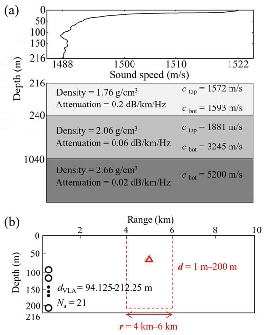
Figure 2.
Schematic diagram of simulation model: (a) the environmental model; (b) source–receiver configuration. The circles indicate hydrophones, and the dots mean the omitted hydrophones.
The sound pressure is assumed as a function of the source–receiver range. The configuration of the source and receiver is shown in Figure 2b. The receiver is a VLA configured identically to VLA in the SWellEx-96 experiment: 21 array elements are distributed between depths of 94.125 m and 212.25 m, array aperture is 118.125 m, and element spacing is about 5.6 m. The potential region for sources is defined as follows: the horizontal range extends from 4 km to 6 km with a grid spacing of 2.5 m, and the depth varies from 1 m to 200 m with a grid spacing of 1 m. The sound source positions are selected within the potential source domain and are individually specified for different simulations. The source frequency is set to [49,64,79,94,112,130,148,166,201,235,283,338,388] Hz, which is consistent with the deep source frequency in the SWellEx-96 Event S5 experiment. During the construction of the sound propagation metamodel, a uniform design method is applied to generate sample points. For the training set, the range sampling interval is set to 0.1 km and the depth sampling interval is set to 8 m. For the validation and test sets, the range sampling interval is set to 0.2 km while the depth sampling interval is set to 20 m.
During the investigation of the robustness to noise, different SNRs are achieved by adding appropriate Gaussian additive noise to the simulated complex pressure signals received. Since the sound source is moving within the range, and the source level is assumed to remain constant during its motion, the received sound pressure level decreases as the range increases. To simulate this condition, the SNR is defined over the farthest range interval between the source and the receiver
where represents the sound pressure signal received by the th element of the array at the farthest source–receiver range, and is the noise variance.
3.2. Main Results
Localization simulations for single and dual sound source are carried out using both the conventional PTR and PTR-MM. These simulations are performed under various key environmental mismatch parameters and different SNRs. The main results for sound source localization simulations are presented below.
3.2.1. Effect of Ocean Environment Parameter Mismatches
Figure 2a illustrates a range-independent shallow water waveguide model that incorporates 14 ocean environmental parameters. Since the effects of mismatches in these parameters on the TR method vary, a sensitivity analysis of PTR to 14 environmental parameters is first performed in this section. The sensitivity analysis goal is to find the environmental parameters whose mismatches have the most significant effects on source localization. The source for the sensitivity analysis is located at (5 km, 54 m), and the other configurations for the simulation are illustrated in Figure 2b. The sound pressure generated by the source at the array and the acoustic Green’s functions between the potential source region field points and the array elements are both obtained by KRAKEN. The values of the 14 ocean environmental parameters are detailed in Table 2. Different ocean environment conditions are achieved by modifying the environmental file of the KRAKEN model.
Table 2.
Ocean environmental parameter values for sensitivity analysis of source localization performance.
By applying Equation (12) to the sound pressure at the array and the Green’s functions between the potential source region points to the array elements, a TR field is obtained of the TRM. And the focusing localization performance of this TRM is quantified by focal bias (FB). Figure 3 illustrates the sensitivity analysis results of FB with respect to the 14 ocean environmental parameters, where the red dashed line indicates the default values for these parameters. The results of Figure 3 reveal that variations in 12 of the environmental parameters have no impact on FB, but the water layer depth and the sediment layer upper speed are found to significantly affect FB within the considered range. These results indicate that the water layer depth and the sediment layer upper speed are the most critical for the localization performance of the TRM in source localization by PTR.
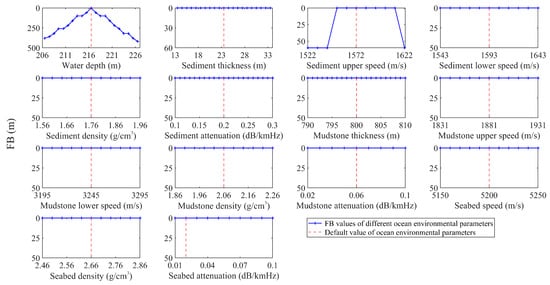
Figure 3.
Sensitivity analysis results of FB with respect to 14 ocean environmental parameters.
Next, PTR and PTR-MM are applied to study the focusing and localization of the sound source located at (5 km, 54 m) under mismatches in the water layer depth and the sediment upper speed. When water layer depth has a mismatch, a sound propagation model with a 226.5 m water layer depth for PTR is used, while all the other ocean environmental parameters remain as given in Table 2. When the sediment upper speed has a mismatch, this speed of the sound propagation model is set to 1622.3 m/s with the other parameters still following Table 2. In contrast, the sound propagation model for PTR-MM is a data-driven metamodel constructed by the sound field data without mismatches, and the training and validation sets are selected as described in Section 3.1. The sound field data of both PTR and PTR-MM are simulated by KRAKEN with different environmental parameters.
Figure 4 illustrates the source localization results of PTR and PTR-MM under these environmental parameter mismatches. Figure 4a,b show that both the water layer depth and the sediment upper speed mismatches lead to significant range bias between focal point and source position when employing PTR. In addition, large sidelobe interference appears near the focal point in both cases. The water layer depth mismatch has a more pronounced effect on the sound source localization accuracy of PTR. Figure 4c clearly demonstrates that PTR-MM accurately localizes the sound source and avoids the sidelobe interference that also affects the source localization. The unbiased source localization of PTR-MM is attributed to the fact that its sound propagation model is derived from a metamodel trained on actual ocean sound field data, ensuring that there is no mismatch between the data-driven sound propagation metamodel and the actual ocean environment.
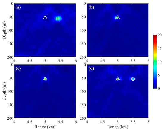
Figure 4.
Source localization results of PTR and PTR-MM under ocean environmental parameter mismatch: (a) PTR with water depth mismatch; (b) PTR with sediment upper speed mismatch; (c) single source using PTR-MM; (d) dual sources using PTR-MM. The white triangles and circle indicate source position.
Additionally, the capability of PTR-MM to simultaneously localize multiple sound sources is further investigated. In the dual-source condition, two coherent sound sources operating at the same frequency are located at positions (5 km, 54 m) and (5.5 km, 54 m), respectively. As illustrated in Figure 4d, PTR-MM accurately localizes both coherent sources. Moreover, the normalized sound intensity derived from the TR process exhibits a distinct contrast between the focal peak amplitudes corresponding to the two sources. This noticeable difference in peak strengths is attributed to the geometric spreading and environmental attenuation effects inherent in sound propagation.
To demonstrate the stability of the localization performance of PTR-MM, the localization of multiple single sources and dual sources is further investigated by PTR-MM. Figure 5 shows the source–receiver array configurations for the study of source localization stability. A total of 303 sources, 101 each at 10 m, 50 m, and 150 m depth, are selected as test sources when studying the localization stability of single sources in the range dimension, as shown in Figure 5a. A total of 150 sources at 4.5 km, 5 km, and 5.5 km range are chosen as test sources for the localization stability studying of a single source in the depth dimension, as shown in Figure 5b. Figure 5c illustrates the configuration of multiple dual sources: 50 test sources (test source 1) are uniformly distributed at a depth of 9 m over a range from 4.02 km to 5 km, and another 50 test sources (test source 2) are uniformly distributed at a depth of 54 m over a range from 5.02 km to 6 km.
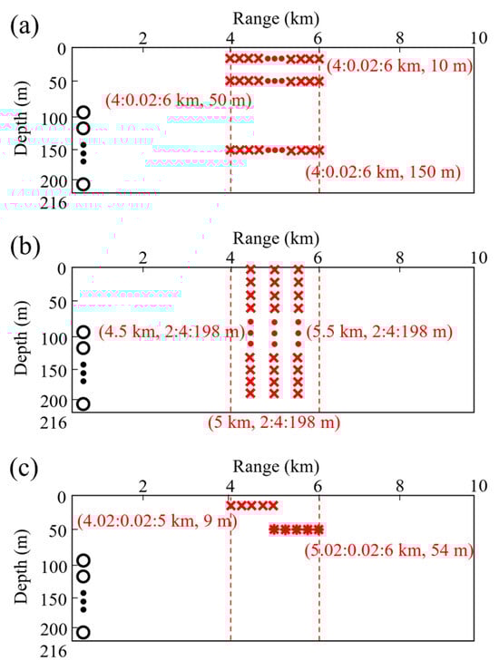
Figure 5.
Source–receiver array configurations for the study of source localization stability: (a) range localization stability of a single source; (b) depth localization stability of a single source; (c) dual-source localization stability. The circles indicate hydrophones, the crosses and asterisks indicate test sources, and the dots mean the omitted hydrophones or test sources.
The range and depth localization results for multiple single sources are shown in Figure 6, while those for multiple dual sound sources are presented in Figure 7. As observed from the results in Figure 6 and Figure 7, the predicted source ranges and depths of PTR-MM closely match the actual source positions for single and dual sources. This result indicates that the proposed method is capable of localizing one or multiple sources at various ranges and depths and demonstrates strong stability in localization performance. Further analysis of the range localization results in Figure 6a and Figure 7a reveals a piecewise pattern, where each segment exhibits a range interval of approximately 0.1 km. This interval corresponds to the sampling interval of the training set used in the metamodel. In other words, the source localization results obtained by PTR-MM tend to align with the training sample positions. This phenomenon can be explained by Figure 8, which presents the transmission loss maps of the potential source region obtained from KRAKEN simulation and the sound propagation metamodel.
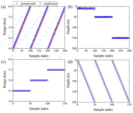
Figure 6.
Multiple single-source localization results for range and depth: (a,b) source localization results for different ranges at three depths; (c,d) source localization results for different depths at three ranges.
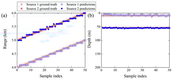
Figure 7.
Multiple dual-source localization results for (a) ranges and (b) depths.
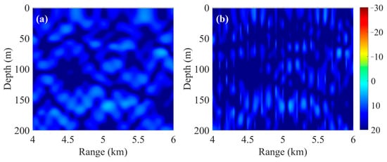
Figure 8.
Sound field transmission loss map in the potential region of the source: (a) KRAKEN; (b) sound propagation metamodel.
As shown in Figure 8, the metamodel exhibits good agreement with the actual sound field in the vicinity of the training sample points but worse agreement outside the sample points. The range sampling interval of the training set must be reduced to further improve the range localization accuracy of the metamodel-based method. However, reducing sampling interval inevitably increases the difficulty of data acquisition and the computational cost of metamodel construction. Therefore, the range sampling interval of the training set should be chosen appropriately based on the desired localization accuracy. Figure 6b and Figure 7b show that PTR-MM achieves higher localization accuracy for deep sources compared to shallow sources. This phenomenon is likely attributable to the increased complexity of the sound field generated by shallow sources near the sea surface, which is influenced by both surface refraction and reflection. The Green’s functions from shallow sources to array elements predicted by the metamodel may deviate more significantly from the actual propagation conditions compared to those of deep sources, resulting in larger localization errors for shallow sources.
3.2.2. Effect of the SNR
In addition to the ocean environmental parameters mismatches, ambient noise is also an important factor that reduces the localization accuracy of PTR method. Therefore, the noise robustness of PTR and PTR-MM is investigated in this section. The sources are located in (4:0.02:6 km, 54 m) among the simulation of noise robustness. The configurations of source frequencies, environmental parameters, array parameters, and metamodel sample points are all consistent with Section 3.1. The noise robustness simulation conditions for PTR and PTR-MM are shown in Table 3, where SNRs are obtained through Equation (14). Range and depth predictions of 101 sources are obtained under the five settings in Table 3, and the MAPE values of these predictions are calculated by Equation (4).
Table 3.
The noise robustness simulation conditions for PTR and PTR-MM.
Figure 9 illustrates the MAPE values of range and depth predictions versus SNRs of the sound pressure signal under 5 conditions. As shown in Figure 9, the MAPE values of range and depth predictions tend to zero when the SNR is larger than −20 dB under 5 conditions. In other words, both PTR and PTR-MM have a good noise robustness when the SNR of sound pressure signals exceeds −20 dB. The condition PTR2 reflects an ideal case where the sound field and the Green’s functions from sources to array elements are perfectly consistent. PTR provides unbiased predictions of the source ranges and depths under condition PTR2, as shown in Figure 9. All the results illustrate that a more precise sound propagation model is necessary for accurate sound source localization at lower SNRs. It is challenging to obtain a conventional sound propagation model that accurately reflects the actual ocean environment, while a data-driven sound propagation metamodel consistent with the actual ocean environment relies on a large amount of acoustic data.
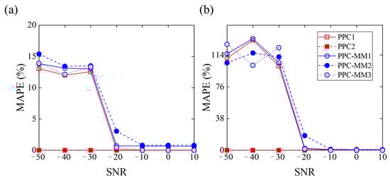
Figure 9.
MAPE values of source predictions versus SNRs under five working conditions: (a) range; (b) depth.
In summary, the results of the noise robustness study indicate that the PTR-MM has a good noise robustness when the SNR of sound pressure signals is above −20 dB. Such robust performance under high noise conditions is sufficient to meet the sound source localization requirements in most ocean environments.
4. Experiments
In this section, the open dataset from the SWellEx-96 experiment is used to investigate the source localization performance of PTR-MM in a real ocean environment. The experiment was conducted in 1996 near San Diego, California, as shown in Figure 10. Source localization experiments are conducted by PTR-MM for multiple single and dual sources based on the experimental dataset. The PTR-MM localization results are also compared with those obtained by PTR. Furthermore, the effect of source frequency (number of frequencies and frequency values) and array parameters (aperture and element spacing) on the localization performance of PTR-MM is studied. Since Event S5 of the SWellEx-96 experiment involves two sources located at different depths and moving along the range dimension (i.e., comprehensive model training data are only available in the range dimension), the source localization problem in this section is essentially a source range prediction problem.
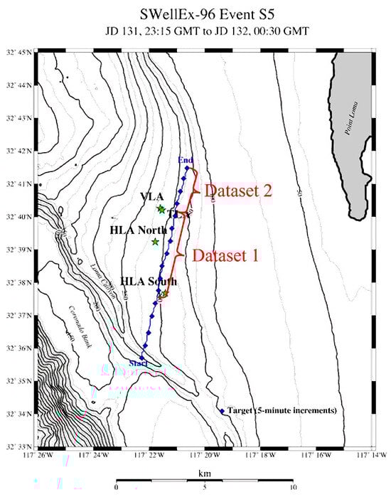
Figure 10.
Event S5 of the SWellEx-96 experiment and datasets division of our experiment.
4.1. Experimental Dataset
The experiment object is the time-domain sound pressure data recorded by the VLA in Event S5 of the SWellEx-96 experiment. The experiment condition and dataset division are illustrated in Figure 10. Table 4 presents the parameter configurations of the deep source (J-15), shallow source (J-13), and VLA. During the experiment, the signal ship started its track south of all of the arrays and proceeded northward at a speed of 5 knots (2.5 m/s), towing a deep source (depth is 54 m) and a shallow source (depth is 9 m). The VLA recorded the full 75 min time-domain sound pressure data during the experiment. These data are transformed into the frequency domain by Equations (2) and (3), resulting in frequency-domain pressure data at the VLA generated by 4500 sources. The frequency-domain pressure data for each source is averaged over four 1 s snapshots. The frequency spectrum recorded by the top hydrophone of the VLA and source–receiver ranges are shown in Figure 11a,c. The frequency spectrum in Figure 11a contains sound pressure signals generated by J-15 and J-13. J-15 and J-13 can be distinguished based on their frequency differences. However, since noise interference prevented clear identification of the J-15 and J-13 pressure signals in Figure 11a, we apply the order-truncate-average algorithm and spectral-peak extraction method [48] to obtain the distinct normalized sound pressure line spectra from Figure 11a, as shown in Figure 11b. In Figure 11b, the red annotations correspond to the signals of J-15, while the blue annotations denote the signals of J-13.
Table 4.
Experimental equipment parameter configurations.
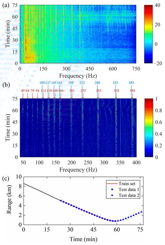
Figure 11.
(a) The frequency spectra recorded on the top hydrophone of VLA, (b) the normalized sound pressure line spectra of J-15 and J-13, and (c) source–receiver ranges during 75 min experiment.
The experimental data are divided into two segments based on the VLA position: one corresponding to the period when the source ship was approaching the array, and the other when it was moving away, as illustrated in Figure 10 and Figure 11c. The final 35 min of the first part are seen as Dataset 1, while all the 16 min of the second part are seen as Dataset 2. In the experiments, data within the same dataset are assumed to share an identical ocean environment, with random noise as the primary interference. In contrast, data from different datasets are associated with different environments, where environmental parameter mismatches dominate. Moreover, the source ship followed similar trajectories during the experimental procedures of Dataset 1 and Dataset 2, with the primary difference being the direction of motion. Given the range-independent characteristics of Event S5, the metamodel trained on Dataset 1 can still be effectively applied to source localization in Dataset 2.
Based on the aforementioned experimental settings, single- and dual-source localization performance experiments are conducted for both deep and shallow sources using Dataset 1. Localization performance experiments for PTR-MM and PTR in different environments are carried out using Datasets 1 and 2, respectively. Furthermore, the effects of frequency and array parameters on the localization performance of PTR-MM are investigated using shallow source data from Dataset 1. The sampling points for the sound propagation metamodel in PTR-MM are selected using a uniform experimental design method, as shown in Table 5. PTR does not require a training or validation set to develop a sound propagation model; instead, its model is simulated by KRAKEN based on the range-independent waveguide environment shown in Figure 2a. The test set for PTR is consistent with that used for PTR-MM.
Table 5.
Dataset configuration of sound propagation metamodel in the PTR-MM experiment.
4.2. Main Results of Source Localization Experiments
PTR-MM is applied to localize a shallow source and a deep source which are both at a range of 3468 m in Dataset 1 environment. The TR sound field relative peak intensities obtained by Equation (13) for the shallow and deep sources are shown in Figure 12, where the relative peak intensity reaches its maximum at a range of 3468 m of the shallow or deep source. This result demonstrates that PTR-MM is able to localize a source at the given range for both shallow and deep sources accurately. A total of 525 sources from the test set of Dataset 1, located at different ranges, are localized using both PTR and PTR-MM. The predicted ranges are presented in Figure 13. These results demonstrate that PTR-MM accurately estimates the ranges of most deep and shallow sources, whereas the range predictions by PTR exhibit significant deviations from the actual source locations. Moreover, the prediction accuracy for shallow sources is slightly higher than that for deep sources, which is consistent with the source localization results in Ref. [33]. Ref. [33] attributes the higher localization accuracy for shallow sources compared to deep sources to differences in signal quality. In this paper, signal continuity is employed as a metric for assessing signal quality, with greater continuity denoting higher quality. As shown in Figure 11b, the shallow-source line spectra exhibit fewer discontinuities than the deep-source spectra, indicating that the shallow-source signal quality exceeds that of the deep-source signal.
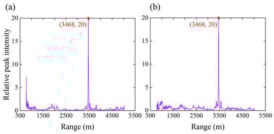
Figure 12.
Relative peak intensity of the PTR sound field by PTR-MM for 3468 m range sources: (a) shallow source; (b) deep source.
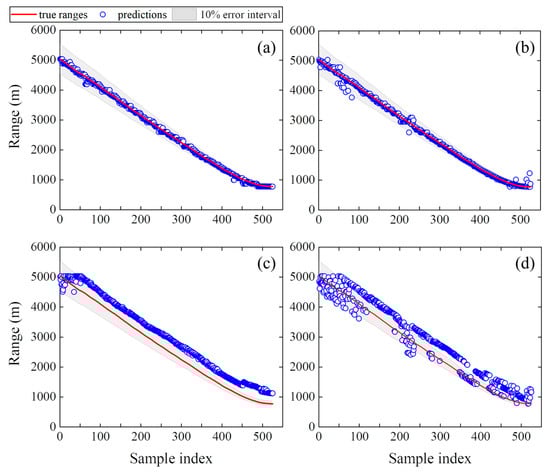
Figure 13.
(a,c) Shallow source and (b,d) deep source range prediction results of the test set in Dataset 1: (a,b) PTR-MM; (c,d) PTR.
PTR-MM is also applied to localize pairs of shallow or deep sources located at ranges of 2640.8 m and 4509.7 m in the Dataset 1 environment. The relative peak intensities of the time-reversed sound field, calculated using Equation (13), for both dual shallow and dual deep sources, are illustrated in Figure 14. As shown in Figure 14, for the dual shallow sources, the first peak in relative peak intensity appears near the VLA, while the second and third peaks are located close to the actual source ranges. For the dual deep sources, the first and second peaks are both positioned near the true source locations. These dual-source localization results confirm that PTR-MM is capable of accurately localizing the target sources while effectively avoiding the influence of peaks near the VLA.
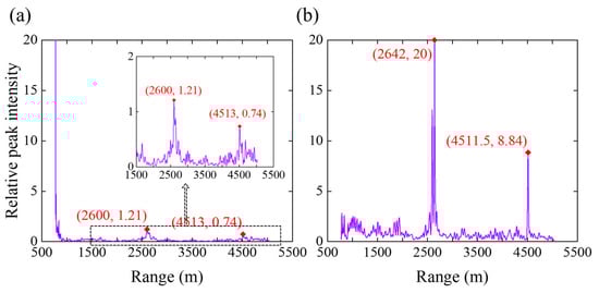
Figure 14.
Relative peak intensity of the PTR sound field by PTR-MM for 2640.8 m and 4509.7 m range dual sources: (a) shallow source; (b) deep source.
In the multiple pairs of sources localization experiments, the first source is drawn from the first 200 sources of Dataset 1 test set, and the second from the 201st to 400th sources of the same test set, yielding 200 pairs of sources. Figure 15 illustrates the range prediction results for the 200 pairs of sources obtained using PTR and PTR-MM. As shown in Figure 15, PTR-MM produces more accurate range predictions for dual sources than PTR, and the vast majority of absolute errors of PTR-MM between the predicted and true ranges are less than 10%. Consistent with the single-source localization results, the prediction accuracy for dual shallow sources is slightly higher than that for dual deep sources. PTR-MM achieves slightly better performance for single-source localization than for dual-source localization by comparing the results in Figure 13a,b and Figure 15a,b.
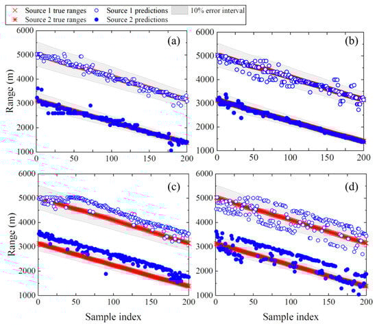
Figure 15.
(a,c) Dual shallow sources and (b,d) dual deep sources range prediction results of the test set in Dataset 1: (a,b) PTR-MM; (c,d) PTR.
In summary, the above results of single-source and dual-source localization experiments by PTR and PTR-MM show that PTR-MM outperforms PTR and remains robust to mismatches. Moreover, PTR-MM is able to simultaneously localize dual sources, but the localization accuracy for the dual sources is slightly lower than that for single sources.
In the aforementioned experiments, the training and test data are drawn from the Dataset 1 ocean environment in which the signal ship moves close to the VLA. Therefore, no errors arise from environmental parameter mismatches between the training and test sets. In order to further investigate PTR-MM localization performance under mismatches of sampling environment, PTR-MM based on a sound propagation metamodel trained on the training set of Dataset 1 is applied to localize 240 single sources in the Dataset 2 test set.
The range predictions for 240 single sources are illustrated in Figure 16. Figure 16a,b illustrates the range predictions of sources in the Dataset 2 test set by PTR-MM based on the training set of Dataset 1. The vast majority of absolute errors between the predicted and true ranges are more than 10% but less than 20%. Figure 16c,d further illustrate the range predictions of sources in the Dataset 2 test set by PTR-MM based on the training set of Dataset 2. The range predictions and the true ranges of 240 sources are in good agreement, except for shallow sources near the VLA. The prediction errors of shallow sources near the VLA are caused by the large sound intensity around the VLA. In summary, the source localization performance of PTR-MM is relatively sensitive to mismatches of sampling environment, and accurate source localization requires a metamodel trained on data obtained from the potential region of target sources.
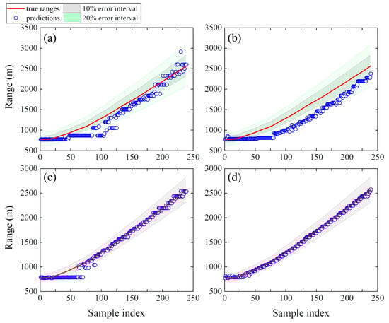
Figure 16.
(a,c) Shallow source and (b,d) deep source range prediction results for the test set in Dataset 2: (a,b) PTR-MM based on training data in Dataset 1; (c,d) PTR-MM based on training data in Dataset 2.
4.3. Effect of Frequency and Array Parameters
In addition to environment parameter mismatch and noise interference, the performance of underwater source localization methods is also affected by source frequency and array parameters. To investigate the effect of source frequency and array parameters on the localization performance of PTR-MM, this section conducts range prediction experiments using shallow source data from Dataset 1. The experiments examine different source frequency parameters (frequency values and the number of frequencies) and array parameters (array aperture and element spacing). The localization performance is evaluated by MAPE. The frequency and array parameter configurations are summarized in Table 6, where Freq represents the frequencies of the shallow source and PVLA represents the position of VLA. In addition, it is known that element 43 of the VLA was damaged during the SWellEx-96 experiment. To facilitate the selection of array aperture and element spacing, only the sound pressure data recorded by elements 8 through 21 of the VLA are used in these experiments.
Table 6.
Frequency and array parameter configurations for studying the effect of frequency and array parameters on sound source localization.
Figure 17 illustrates the MAPE values of range predictions for shallow sources in the test set of Dataset 1 versus different frequency parameters: the MAPE initially increases and then decreases as the frequency increases, while the MAPE remains unchanged with increasing number of frequencies. As demonstrated in Section 4.2, source localization accuracy may also depend on signal quality. Given the pronounced disparity in line spectrum continuity between the shallow and deep sources in Figure 11b, Section 4.2 employs signal continuity as a qualitative metric for signal quality. However, since the line spectra of shallow sources at different frequencies exhibits minimal variation, we introduce a signal quality metric (SQ). SQ is defined as the number of continuous segments in a line spectrum, and the greater SQ values mean the higher signal quality. The data for this section are drawn from Dataset 1, which contain the signal ship operation from 24 min to 59 min. Accordingly, the shallow source line spectra between 24 min and 59 min in Figure 11b are used to calculate SQs. First, the mean pressure values of the shallow source line spectra at 109–385 Hz over the 24 min to 59 min interval are calculated. Second, any pressure data of a line spectrum below the mean value are set to 0 at each frequency. Finally, SQ is the number of transitions from non-zero to zero in the pressure data for each shallow source line spectra at different frequencies. The calculation results of SQs are shown in Figure 17a. Except at 385 Hz, SQ initially decreases and then increases with rising frequency, exhibiting the inverse trend of MAPE. Furthermore, when SQ exceeds 700, the MAPEs converge to approximately 3%. According to the above results, we propose that the frequency dependence for PTR-MM localization performance of shallow sources is likely related to signal quality. As SQ increases, PTR-MM localization performance improves. But there exists a critical threshold beyond which further increases in SQ yield negligible gains in localization accuracy.
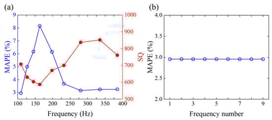
Figure 17.
Range prediction MAPEs of shallow sources for the test set in Dataset 1 versus frequency parameters: (a) frequency value; (b) number of frequencies.
MAPEs of range predictions for shallow sources in the test set of Dataset 1 versus different array parameters is illustrated in Figure 18: MAPE decreases as the aperture increases, while MAPE increases with increasing element spacing. The results above indicate that the localization performance of PTR-MM is significantly influenced by array parameters. A larger array aperture and smaller element spacing enhances its localization accuracy effectively.
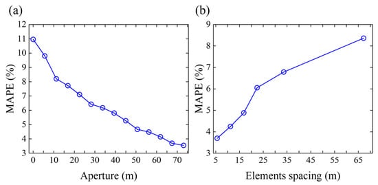
Figure 18.
Range prediction MAPEs of shallow sources for the test set in Dataset 1 versus array parameters: (a) aperture; (b) element spacing.
5. Conclusions
PTR-MM for underwater source localization is proposed to address the environment mismatch problem and, simultaneously, multiple-source localization difficulty. PTR-MM localizes sources by using the focusing properties of the PTR sound field. PTR-MM enhances robustness to environmental mismatch by replacing the conventional sound propagation model with a metamodel during the TR process. Simulation results using KRAKEN for the environment of Event S5 in the SWellEx-96 experiment demonstrate that PTR-MM localizes both single and multiple sources in the simulation environment accurately. The localization performance of PTR-MM is insensitive to mismatches in ocean environmental parameters and exhibits a degree of robustness to noise. Specifically, PTR-MM remains effective under noise interference with an SNR greater than −20 dB. Further validation using data from Event S5 in the SWellEx-96 experiment confirms the effectiveness of PTR-MM in practical underwater source localization applications.
In both the simulation and the experiment, PTR-MM outperforms PTR in terms of localization accuracy. However, the localization performance of PTR-MM degrades significantly under environmental mismatch between training and test data, which requires the metamodel be trained using data collected from an environment consistent with the potential region of the target sources. Moreover, experimental results on the effect of frequency and array parameters indicate that the localization performance of PTR-MM is determined primarily by signal quality and array parameters, rather than source frequency: higher signal quality, larger array aperture, and smaller element spacing contribute to improved localization accuracy of PTR-MM.
For our simulation and experiment, PTR-MM fails when the SNR is less than −20 dB or when the training data are not obtained from the potential region of the target sources. All source localization studies in this work are conducted in one- or two-dimensional spaces, with the size of the training sets for the metamodel kept below 1000 samples. However, as the problem dimension increases or the acoustic environment becomes more complex, the amount of training data required to construct an optimal metamodel inevitably grows. This increase poses challenges for data collection and may reduce the overall feasibility of the proposed method. Therefore, extending the approach to high-dimensional and complex acoustic environments will be a key direction for future research. For example, the PTR-MM could be combined with semi-supervised learning to develop source localization algorithms which are able to learn unlabeled data. Furthermore, a more realistic ocean noise model is important for source localization research. So, the effect of complex and high-intensity ocean noise on the localization performance of PTR-MM will be another key focus of our future research.
Author Contributions
Conceptualization, J.L.; methodology, J.L.; software, J.L.; validation, J.L.; formal analysis, J.L.; investigation, J.L.; resources, S.L.; data curation, J.L.; writing—original draft preparation, J.L.; writing—review and editing, S.L.; visualization, J.L.; supervision, S.L.; project administration, S.L.; funding acquisition, S.L. All authors have read and agreed to the published version of the manuscript.
Funding
This research received no external funding.
Data Availability Statement
The original contributions presented in this study are included in the article. Further inquiries can be directed to the corresponding author.
Conflicts of Interest
The authors declare no conflicts of interest.
References
- Hu, Z.; Huang, J.; Xu, P.; Nan, M.; Lou, K.; Li, G. Underwater Acoustic Source Localization via Kernel Extreme Learning Machine. Front. Phys. 2021, 9, 653875. [Google Scholar] [CrossRef]
- Liu, K.W.; Huang, C.J.; Too, G.P.; Shen, Z.Y.; Sun, Y.D. Underwater Sound Source Localization Based on Passive Time-Reversal Mirror and Ray Theory. Sensors 2022, 22, 2420. [Google Scholar] [CrossRef] [PubMed]
- Dowling, D.R.; Sabra, K.G. Acoustic Remote Sensing. Annu. Rev. Fluid Mech. 2015, 47, 221–243. [Google Scholar] [CrossRef]
- Rossing, T. Springer Handbook of Acoustics; Springer Science & Business Media: New York, NY, USA, 2007. [Google Scholar]
- Bianco, M.J.; Gerstoft, P.; Traer, J.; Ozanich, E.; Roch, M.A.; Gannot, S.; Deledalle, C.A. Machine learning in acoustics: Theory and applications. J. Acoust. Soc. Am. 2019, 146, 3590. [Google Scholar] [CrossRef] [PubMed]
- Carter, G.C. Passive ranging errors due to receiving hydrophone position uncertainty. J. Acoust. Soc. Am. 1979, 65, 528–530. [Google Scholar] [CrossRef]
- Ferguson, B.G.; Lo, K.W. Passive ranging errors due to multipath distortion of deterministic transient signals with application to the localization of small arms fire. J. Acoust. Soc. Am. 2002, 111 Pt 1, 117–128. [Google Scholar] [CrossRef]
- Kulkarni, S.; Thakur, A.; Soni, S.; Hiwale, A.; Belsare, M.H.; Raj, A.A.B. A Comprehensive Review of Direction of Arrival (DoA) Estimation Techniques and Algorithms. J. Electron. Electr. Eng. 2025, 4, 138–186. [Google Scholar] [CrossRef]
- Van Veen, B.D.; Buckley, K.M. Beamforming: A versatile approach to spatial filtering. IEEE ASSP Mag. 1988, 5, 4–24. [Google Scholar] [CrossRef]
- Karaman, M.; Pai-Chi, L.; O’Donnell, M. Synthetic aperture imaging for small scale systems. IEEE Trans. Ultrason. Ferroelectr. Freq. Control 1995, 42, 429–442. [Google Scholar] [CrossRef]
- Johnson, D.H. The application of spectral estimation methods to bearing estimation problems. Proc. IEEE 1982, 70, 1018–1028. [Google Scholar] [CrossRef]
- Schmidt, R. Multiple emitter location and signal parameter estimation. IEEE Trans. Antennas Propag. 1986, 34, 276–280. [Google Scholar] [CrossRef]
- Baggeroer, A.B.; Kuperman, W.A.; Mikhalevsky, P.N. An overview of matched field methods in ocean acoustics. IEEE J. Ocean. Eng. 1993, 18, 401–424. [Google Scholar] [CrossRef]
- Bucker, H.P. Use of calculated sound fields and matched-field detection to locate sound sources in shallow water. J. Acoust. Soc. Am. 1976, 59, 368–373. [Google Scholar] [CrossRef]
- Yonak, S.H.; Dowling, D.R. Parametric dependencies for photoacoustic leak localization. J. Acoust. Soc. Am. 2002, 112, 145–155. [Google Scholar] [CrossRef] [PubMed]
- Gerstoft, P. Inversion of seismoacoustic data using genetic algorithms and a posteriori probability distributions. J. Acoust. Soc. Am. 1994, 95, 770–782. [Google Scholar] [CrossRef]
- Jackson, D.R.; Dowling, D.R. Phase conjugation in underwater acoustics. J. Acoust. Soc. Am. 1991, 89, 171–181. [Google Scholar] [CrossRef]
- Kuperman, W.A.; Hodgkiss, W.S.; Song, H.C.; Akal, T.; Ferla, C.; Jackson, D.R. Phase conjugation in the ocean: Experimental demonstration of an acoustic time-reversal mirror. J. Acoust. Soc. Am. 1998, 103, 25–40. [Google Scholar] [CrossRef]
- Song, H.C.; Kuperman, W.A.; Hodgkiss, W.S. A time-reversal mirror with variable range focusing. J. Acoust. Soc. Am. 1998, 103, 3234–3240. [Google Scholar] [CrossRef]
- Fink, M.; Prada, C. Acoustic time-reversal mirrors. Inverse Probl. 2001, 17, R1–R38. [Google Scholar] [CrossRef]
- Kim, J.S.; Song, H.C.; Kuperman, W.A. Adaptive time-reversal mirror. J. Acoust. Soc. Am. 2001, 109 Pt 1, 1817–1825. [Google Scholar] [CrossRef]
- Walker, S.C.; Roux, P.; Kuperman, W.A. Synchronized time-reversal focusing with application to remote imaging from a distant virtual source array. J. Acoust. Soc. Am. 2009, 125, 3828–3834. [Google Scholar] [CrossRef] [PubMed]
- Zhang, T.; Yang, K.; Ma, Y. Matched-field localization using a virtual time-reversal processing method in shallow water. Chin. Sci. Bull. 2011, 56, 743–748. [Google Scholar] [CrossRef]
- Tan, T.W.; Godin, O.A.; Brown, M.G.; Zabotin, N.A. Characterizing the seabed in the Straits of Florida by using acoustic noise interferometry and time warping. J. Acoust. Soc. Am. 2019, 146, 2321. [Google Scholar] [CrossRef]
- Fu, Y.; Yu, Z. A Low SNR and Fast Passive Location Algorithm Based on Virtual Time Reversal. IEEE Access 2021, 9, 29303–29311. [Google Scholar] [CrossRef]
- Godin, O.A.; Uzhansky, E.M.; Tan, T.; Katsnelson, B.G.; Tan, D.Y.; Renucci, T.; Voyer, A.; McMullin, R.M. Acoustic characterization of the seabed with a single-element time-reversal mirror. Appl. Acoust. 2023, 210, 109442. [Google Scholar] [CrossRef]
- Im, S.; Lee, J.W.; Han, T.; Ohm, W.S. A single-channel virtual receiving array using a time-reversal chaotic cavity. J. Acoust. Soc. Am. 2023, 154, 1401–1412. [Google Scholar] [CrossRef]
- Niu, H.; Ozanich, E.; Gerstoft, P. Ship localization in Santa Barbara Channel using machine learning classifiers. J. Acoust. Soc. Am. 2017, 142, EL455–EL460. [Google Scholar] [CrossRef]
- Niu, H.; Reeves, E.; Gerstoft, P. Source localization in an ocean waveguide using supervised machine learning. J. Acoust. Soc. Am. 2017, 142, 1176–1188. [Google Scholar] [CrossRef]
- Diniz, P.; Calazan, R. Integrating modeled environmental variability into neural network training for underwater source localization. J. Acoust. Soc. Am. 2023, 153, 3201. [Google Scholar] [CrossRef]
- Ferguson, E.L.; Williams, S.B.; Jin, C.T. In Sound source localization in a multipath environment using convolutional neural networks. In Proceedings of the 2018 IEEE International Conference on Acoustics, Speech and Signal Processing (ICASSP), Calgary, AB, Canada, 15–20 April 2018; pp. 2386–2390. [Google Scholar]
- Chen, R.; Schmidt, H. Model-based convolutional neural network approach to underwater source-range estimation. J. Acoust. Soc. Am. 2021, 149, 405–420. [Google Scholar] [CrossRef]
- Wang, Y.; Peng, H. Underwater acoustic source localization using generalized regression neural network. J. Acoust. Soc. Am. 2018, 143, 2321–2331. [Google Scholar] [CrossRef] [PubMed]
- Huang, Z.; Xu, J.; Gong, Z.; Wang, H.; Yan, Y. Source localization using deep neural networks in a shallow water environment. J. Acoust. Soc. Am. 2018, 143, 2922–2932. [Google Scholar] [CrossRef] [PubMed]
- Lataniotis, C.; Wicaksono, D.; Marelli, S.; Sudret, B. UQLab User Manual—Kriging (Gaussian Process Modeling); Report UQLab-V2.0-105; Chair of Risk, Safety and Uncertainty Quantification, ETH Zurich: Zurich, Switzerland, 2022. [Google Scholar]
- Luegmair, M.; Dantas, R.; Schneider, F.; Müller, G. Gaussian Process Surrogate Models for Vibroacoustic Simulations; SAE International: Warrendale, PA, USA, 2024. [Google Scholar]
- Kim, J.S.; Jeong, U.C.; Kim, D.W.; Han, S.Y.; Oh, J.E. Optimization of sirocco fan blade to reduce noise of air purifier using a metamodel and evolutionary algorithm. Appl. Acoust. 2015, 89, 254–266. [Google Scholar] [CrossRef]
- Du, X.; Fu, Q. Surrogate model-based multi-objective design optimization of vibration suppression effect of acoustic black holes and damping materials on a rectangular plate. Appl. Acoust. 2024, 217, 109837. [Google Scholar] [CrossRef]
- Aoun, C.G.; Lagadec, L.; Habes, M. An extended modeling approach for marine/deep-sea observatory. In International Conference on Advanced Machine Learning Technologies and Applications; Springer International Publishing: Cham, Switzerland, 2022; pp. 502–514. [Google Scholar]
- Jenkins, W.F.; Gerstoft, P.; Park, Y. Geoacoustic inversion using Bayesian optimization with a Gaussian process surrogate model. J. Acoust. Soc. Am. 2024, 156, 812–822. [Google Scholar] [CrossRef]
- Goupy, A. A Spectral Approach of Multi-Scale Metamodelling Applied to Acoustic Propagation. Doctoral Dissertation, Université Paris-Saclay, Gif-sur-Yvette, France, 2021. [Google Scholar]
- Cheng, L.; Li, M. Underwater source localization based on dynamic weight meta-learning. In Proceedings of the 3rd International Conference on Signal Processing, Computer Networks and Communications, Sanya, China, 22–24 December 2024; pp. 107–112. [Google Scholar]
- Jenkins, W.F.; Gerstoft, P.; Park, Y. Bayesian optimization with Gaussian process surrogate model for source localization. J. Acoust. Soc. Am. 2023, 154, 1459–1470. [Google Scholar] [CrossRef]
- Marelli, S.; Sudret, B. UQLab: A framework for uncertainty quantification in Matlab. In Proceedings of the 2nd International Conference on Vulnerability, Risk Analysis and Management (ICVRAM2014), Liverpool, UK, 13–16 July 2014; pp. 2554–2563. [Google Scholar]
- Godin, O.A.; Katsnelson, B.G.; Qin, J.; Brown, M.G.; Zabotin, N.A.; Zang, X. Application of time reversal to passive acoustic remote sensing of the ocean. Acoust. Phys. 2017, 63, 309–320. [Google Scholar] [CrossRef]
- Porter, M.B. The KRAKEN Normal Mode Program. Available online: https://oalib-acoustics.org/website_resources/AcousticsToolbox/Kraken.pdf (accessed on 17 April 2025).
- Murray, J.; Ensberg, D. The SWellEx-96 Experiment. Available online: http://swellex96.ucsd.edu (accessed on 17 April 2025).
- Nielsen, R.O. Sonar Signal Processing; Artech House Inc.: London, UK, 1991. [Google Scholar]
Disclaimer/Publisher’s Note: The statements, opinions and data contained in all publications are solely those of the individual author(s) and contributor(s) and not of MDPI and/or the editor(s). MDPI and/or the editor(s) disclaim responsibility for any injury to people or property resulting from any ideas, methods, instructions or products referred to in the content. |
© 2025 by the authors. Licensee MDPI, Basel, Switzerland. This article is an open access article distributed under the terms and conditions of the Creative Commons Attribution (CC BY) license (https://creativecommons.org/licenses/by/4.0/).