Smart Maritime Transportation-Oriented Ship-Speed Prediction Modeling Using Generative Adversarial Networks and Long Short-Term Memory

Abstract

Ship-speed prediction is an emerging research area in marine traffic safety and other related fields, occupying an important position with respect to these areas. At present, the effectiveness of techniques used in in time-series forecasting methods in ship-speed prediction is poor, and there are accumulated errors in long-term forecasting, which is limited in its processing of ship-speed information combined with multi-feature data input. To overcome this difficulty and further optimize the accuracy of ship-speed prediction, this research proposes a new deep learning framework to predict ship speed by combining GANs (Generative Adversarial Networks) and LSTM (Long Short-Term Memory). First, the algorithm takes an LSTM network as the generating network and uses the LSTM to mine the spatiotemporal correlation between nodes. Secondly, the complementary characteristics linked between the generative network and the discriminant network are used to eliminate the cumulative error of a single neural network in the long-term prediction process and improve the prediction accuracy of the network in ship-speed determination. To conclude, the Generator–LSTM model advanced here is used for ship-speed prediction and compared with other models, utilizing identical AIS (automatic identification system) ship-speed information in the same scene. The findings indicate that the model demonstrates high accuracy in the typical error measurement index, which means that the model can reliably better predict the ship speed. The results of the study will assist maritime traffic participants in better taking precautions to prevent collisions and improve maritime traffic safety.

1. Introduction

1.1. Introductory Context

Over the past few years, with recent vigorous advancements in maritime transportation and trade, the investigation into intelligent ships has emerged as a key area of research in the shipping field. One crucial aspect of this research is the accurate prediction of ship speed, which plays a vital role in ensuring the continuous growth and stability of the shipping sector [1]. Therefore, it is necessary to make good predictions of ship speed.

Researchers worldwide have conducted extensive studies on the prediction of ship navigation dynamics, including factors such as speed and trajectory [2]. As the relevant applied technologies have advanced, there have been significant changes in forecasting methods at the technical level, which have transitioned from empirical formulas and physical approaches to data-driven models [3]. Early researchers constructed empirical formulas for speed within a specific tonnage range by fitting a collection of operational constants established from actual data, and some of these methods are still in use today. Li et al. utilized AIS (automatic identification system) data to model and predict ship trajectories. For this task, they employed five machine learning techniques: Kalman Filter (KF), Support Vector Regression (SVR), Backpropagation Network (BP), Gaussian Process Regression (GPR), and Random Forest (RF) [4]. In addition, seven deep learning approaches were used: Recurrent Neural Networks (RNNs), Long Short-Term Memory (LSTM), Gated Recurrent Unit (GRU), Bidirectional LSTM (Bi-LSTM), Sequence-to-Sequence (Seq2seq), Bidirectional GRU (Bi-GRU), and Transformer. The effectiveness of each method was demonstrated under various maritime conditions.

AI has been crucial in advancing the autonomous navigation of unmanned vessels, and collision risk has become a major concern as the shipping industry expands, and the number of ships rises, especially autonomous vessels functioning in intricate environments [5]. Aristov et al. focused on maritime ports and their associated terminals, using several ports along the east coast of the United States as case studies. They traced the historical routes of container ships and accurately mapped the areas in which ships docked within terminals. This research provided valuable insights into ship scheduling and offered significant value to stakeholders in the supply chain industry, contributing to both theoretical and practical applications in maritime logistics [6]. In addition, some scholars have used the existing knowledge of ship dynamics and fluid mechanics to build a physical model of a ship’s sailing motion in wind and waves, based on the descriptions of ship propulsion force and resistance, aiming to predict ship speed.

This paper presents a new deep learning framework for ship-speed prediction by combining GANs (Generative Adversarial Networks) and LSTMs. Unlike other deep learning models such as the GRU, LSTM, and WAGCN, this model takes geospatial dependence into consideration. Compared with the GAN–GRU and GAN–WAGCN combined with GAN, the proposed model can improve the prediction effectiveness by enhancing the diversity of models, capturing more complex data patterns, and improving the accuracy and stability of the prediction. First, the algorithm takes an LSTM network as the generating network and uses an LSTM to mine the spatiotemporal correlation between nodes. Secondly, the complementary characteristics linked between the generative network and the discriminant network are used to eliminate the cumulative error of a single neural network in the long-term prediction, optimizing and boosting the prediction accuracy of the network in ship-speed determination. Ultimately, the proposed Generator–LSTM model is used for vessel speed prediction, and compared with other models, using the same AIS ship-speed information in the same scene. The key contributions of this paper are following three aspects: (1) a ship-speed-prediction model which enhances model diversity is proposed; (2) more spatial features and complex data patterns can be captured by introducing GAN models; (3) the Generator–LSTM is verified using the data of two different types of ship scenarios. The organization of the paper is as follows: Section 2 covers the related research in speed prediction. Section 3 covers the specifics of the approach in this study. Section 4 presents the experimental settings and analyzes the results. Finally, Section 5 summarizes the research.

As sensor reception capabilities and computational power continue to improve, data-driven, technology-based speed-prediction methods have become increasingly feasible [7]. Previously, various relevant ship trajectory prediction tactics and techniques for ship-speed prediction have been proposed, among which deep learning methods have attracted significant attention due to the ability of this approach to take into account key factors and adjust to complex situations; nevertheless, the use of this technique in practice has been limited due to the insufficient extraction of environmental factors and feature data. Pensado et al. presented a real-time trajectory optimizer for shore-to-ship operations utilizing Unmanned Aerial Vehicles (UAVs), aiming to enhance the efficiency of the transportation system by leveraging UAVs for parcel deliveries to offshore ships, streamlining logistics and reducing delivery times [8].

1.2. Literature Review

With recent increases in maritime traffic flow and frequent navigation activities, ship collisions, as well as groundings and other accidents, have been occurring. In helping to mitigate such safety concerns, high-precision and stable ship trajectory prediction plays a vital role in the development of accident prevention technologies for the maritime IoT industry. Magalhães et al. considered ship trajectory prediction a challenge due to the difficulties that traditional deep learning techniques have in capturing complex changes in trajectories. To overcome this obstacle, they used the deep learning network encoded by Geohash to predict ship trajectory using clustering AIS data in an approach developed for the IoT industry, and applied a density-based, noise-aware spatial clustering algorithm to perform cluster analysis on the trajectories. Trajectory data across different categories were entered into the LSTM optimization network for the purpose of Geohash coding training [9]. A majority of the available research has indicated that deep learning-based methods for ship-speed prediction have been incorporated into the industry, significantly enhancing prediction accuracy and aiding maritime professionals in identifying potential safety risks. Padmavathi et al. proposed the use of the Kolmogorov–Arnold Networks (KAN) algorithm for prediction, which has effectively improved accuracy. The performance of the proposed method is evaluated using various metrics, including MAE, MSE, RMSE, and MAPE, based on the AIS dataset [10].

Accurate prediction using deep learning methods based on AIS data has become a key focus in modern maritime transportation research. Donandt et al. focused on inland Vessel Traffic Planning (VTP) and applied Gaussian Mixture Models to a fused dataset of AIS and discharge measurements. This approach generated multi-modal distribution curves that capture typical lateral vessel positioning in the fairway, as well as dislocation speeds along the waterway [11]. Data-driven models can integrate unmodeled physical phenomena into physical models, resulting in improved predictions, provided that the data and algorithms are used rationally. With the developments in the capabilities of computers, the utilization of AIS data allows for the estimation of ship speed. AIS is a ship-based proportional communication device utilized for both navigation and collision prevention. Some scholars have proposed a Support Vector Regression model based on adaptive chaotic differential evolution; this approach selected speed, course, time, latitude, and longitude as sample features from the AIS data, aiming to predict ship trajectory [12]. Owing to its extensive coverage and abundant information, including static information, dynamic information, and navigation-related information, AIS is widely used in ship-speed prediction. AIS is considered to be a key data source, in that it represents maritime traffic spatially and temporally in the context of marine spatial planning; it is widely used in ship-speed prediction research, and can offer informational support for navigation risk assessment.

Sigillo et al. tackled the challenging problem of vessel route forecasting using a vast number of AIS records. They proposed a novel deep learning architecture, SeaFormer, which leveraged transformer modules to capture long-term dependencies in the data. This approach enabled the forecasting of vessel routes even several hours ahead, improving the accuracy and timeliness of maritime navigation predictions [13]. Gülsoylu et al. addressed the problem by developing a technique that fused AIS data with data describing the vessels detected in the images to create enriched datasets. This fusion combined visual data with vessel-related information, such as type, size, speed, and direction, providing a more comprehensive understanding of vessel behavior and improving analysis capabilities [14]. In addition, AIS data are also used to predict ship tracks under uncertain conditions, extract ship-movement patterns, and identify abnormal ship behavior, in order to reduce threats to other nearby ships. Before using AIS data, it should be noted that because the communication channels of AIS are concentrated in traffic-intensive waterways, the transmission rates associated with the AIS data will change. Based on the navigation status of a given ship, there will be anomalies in the original AIS data, so data cleaning and interpolation are needed [15].

In recent years, the study of ship trajectory prediction has been developed rapidly due to the rich ship-movement information (including ship position, speed, course, and heading) provided by AIS [16]. Various data-driven approaches have been developed, including SVM (Support Vector Machines), BP, and LSTM. Ship track prediction contributes significantly to the maintenance of traffic safety in busy waterways. Conventional forecasting techniques often ignored the complex spatiotemporal interactions and the built-in collision prevention actions that take place during encounters between multiple vessels, resulting in lack of precision in the trajectory forecasting associated with the interaction. Pappagallo et al. focused on implementing a ’Port Classifier,’ evaluating several models, including Conv1D, MLP, and LSTM, on AIS trajectories labeled through heuristic algorithms. Their study showed promising results, with Conv1D demonstrating superiority in port classification tasks. They also conducted an Exploratory Data Analysis (EDA) to gain a deeper understanding of the data, further improving the classification performance [17]. As described in case studies, neural networks combined with GANs have demonstrated the capability to develop navigation rules beyond the current regulations, and provide valuable insights for improving safety in offshore operations.

Ship speed is a critical factor in the decision-making processes of maritime transportation, such as determining ETA (estimated time of arrival), estimating fuel usage, planning collision-free routes, and so on. Nevertheless, the speed of the ship is occasionally anomalously reduced because of increased wind/wave friction and decreased propulsion efficiency, so accurate ship-speed forecasting demands a thorough understanding of drag, propulsion, machinery, and more. Various models have been created for the prediction of ship speed; these could be classified as data-driven or semi-data-driven formulas, including computational liquid dynamic, as well as experimental, simulations [18]. In addition to the above methods, dynamic prediction utilizing time-series data has also found important uses in the shipping industry. Certain researchers have used AIS data and artificial intelligence approaches to forecast ship speed, and the prediction accuracy has been improved [19].

There are, occasionally, obvious present or potential trends in ship sailing states and marine meteorological conditions, and constructing time series for relevant predictions may achieve good results [20]. Comprehending the dynamics between a ship and its surroundings allows for optimal path prediction, which is essential for enhancing the safe navigation of autonomous vessels. Predicting future trajectories is a highly complex task because of the inherent uncertainties and the intricate temporal and spatial relationships between various ships. Nonetheless, current approaches disregard the continuity and cross-border aspects of ship-to-ship impacts. Chen et al. proposed a novel ship route planning method that took into account various factors, such as weather conditions and carbon emissions. Their research findings aimed to assist the maritime community in making ship routing decisions that were more reasonable and environmentally conscious under different navigation conditions, enhancing efficiency and sustainability in maritime operations [21]. Ourc et al. introduced a practical framework for predicting risky close encounters and gray-zone interactions, using historical AIS data and LSTM networks. Their methodology developed an extensive encounter model that identified ship-to-ship interactions and classified them as risky, gray-zone, or non-risky encounters, based on ship domain violations. This approach enhanced safety by providing early detection and classification of potential risks in maritime navigation [22]. Shin et al. studied port ship trajectory forecasting using a deep learning technique method for maritime data preprocessing and berthing-side integration, and this maritime special data preprocessing technology improved the performance of the model [23]. The model was trained using AIS data and the mean square error was used as an evaluation index, aiming to forecast future outcomes for sailing ship location.

Yang et al. combined the Transformer model, which was popular within the domain of artificial intelligence, with the traditional KF model, and proposed a new flight-path prediction model [24]. The experimental results showed that, compared to the use of a conventional method, this approach offered improved prediction accuracy and superior parallel processing of sequence data. Mehri et al. introduced a ship trajectory prediction approach utilizing RNN. For the data preprocessing stage, a method based on symmetric segmented path distance was developed to mitigate the impacts of redundant data and noise. For the prediction process, an RNN model based on the gated cycle unit was designed, attempting to achieve effective and timely prediction of ship position details [25].

In addition, the sailing sea area, loading state, and ship-type of the ship are obviously different for each voyage, which causes inconsistent data distribution and makes it difficult to extend the trained model to the new data [26]. Xian et al. studied a received signal strength (RSS)-based three-dimensional (3D) drowning target localization that simultaneously considered the absorption effect, uncertain transmission power (UTP), and the time-varying path loss exponent (PLE) for underwater search and rescue missions, induced by the frequent occurrence of maritime accidents [27]. Researchers in similar areas have been working on developing a series of ship-speed prediction models that are more accurate and robust, aiming to effectively monitor the future navigation statuses of ships. These models aim to enhance the safety and efficiency of maritime navigation by providing timely and reliable predictions, allowing for better decision-making in real-time navigation scenarios [28,29].

2. Materials and Methods

2.1. Research Area

It is known that relative to the world-wide carrying capacity for tankers, the present number of vessels constitutes less than 30%, while the counterpart for container ships is 13.5%. More specifically, both tankers and container ships are commonly used for the transfer of cargo goods within the maritime industry. Thus, tankers transport liquid cargoes, especially crude oil and chemicals, and their maritime safety is particularly important. Ship speed is a key parameter of maritime navigation safety. The ship-speed predictions for oil tankers and container ships play an important role in ensuring maritime safety [30]. Accurate ship-speed prediction can help the crew to perform better navigation planning, reduce risks, and improve efficiency [31]. Weather conditions, ship load, marine environment, and ship performance will directly or indirectly affect ship speed.

Actions relating to modern tankers and container ships can also be predicted using artificial intelligence and machine learning algorithms. These technologies build complex predictive models by analyzing large amounts of historical data, such as ship speed, weather, sea state, etc. AI can automatically recommend the best ship speed based on real-time input of weather data and information relating to the marine environment.

2.2. Methodology

2.2.1. AIS Data Preprocessing

The data we used is derived from AIS information, which contains some ship-related information, such as MMSI (Maritime Mobile Service Identification), location, heading and speed. Depending on the speed and route, the intervals between messages sent varies from 2 s to 3 min. The AIS data used in this study were located at https://marinecadastre.gov/ais/ (accessed on 24 March 2025), and were download from the website [32].

In terms of speed prediction, the original AIS information was gathered first. Then, five steps, comprising data outlier detection, speed statistics extraction, speed information for data interpolation determination, uniform interval processing, and data standardization, were carried out. Speed information was used for data interpolation, uniform interval processing, and data standardization. The data preprocessing workflow is illustrated in Figure 1.

After assigning the data as the input label for model training, anomaly detection is initially applied to identify deviant samples prior to executing de-duplication procedures. Following the initial data acquisition, velocity vectors are computationally derived, with subsequent application of threshold-based filtering to eliminate non-compliant kinematic measurements then performed. We used a low-pass filter to smooth out noise, especially in cases of drastic changes in speed or position, in order to reduce the interference of short-term abnormal fluctuations in model training. Furthermore, we have also enhanced the robustness of the model through data augmentation techniques, enabling it to better handle errors caused by noise.

AIS data play an important role in ship monitoring and navigation analysis, especially in applications such as ship-speed prediction. AIS data have some inherent limitations, such as missing values, transmission errors, and other problems, all of which would affect the accuracy and reliability of ship-speed prediction. Missing values in AIS data may lead to the discontinuity of the time series, affecting the training and prediction accuracy of the model. In this paper, the missing values are filled through linear interpolation, and when using time-series prediction models (such as the LSTM, GRU, etc.), the processing of missing data is taken as a specific input feature in optimizing the model. Transmission errors may lead to outliers or inconsistencies in AIS data, especially data that are abnormal in terms of speed and heading. This kind of error will directly affect the training of the ship-speed prediction model and may lead to the deviations in the prediction results. This paper identified and corrected the transmission errors by performing outlier detection on the data.

In the container-ship experiment scenario, due to the high loading and unloading speeds and short port-stop times of container ships, most of them utilize high speeds. In recent years, in order to save energy, a more economical speed was generally adopted, which was about 18 nautical miles per hour, while the speed of a container ship in short-distance coastal navigation is only about 10 nautical miles per hour. Therefore, data with velocity values outside the interval 10 ≤ v ≤ 18 knots were removed in the data preprocessing for the container-ship experiment scenarios. In the tanker experiment scenario, since the speed of the tanker is generally 13 to 17 knots, the data associated with speed values outside the interval 13 ≤ v ≤ 17 knots were removed in the data preprocessing for the tanker experiment scenarios. Next, the cubic spline interpolation technique was applied to set the interval between each data point to 10s, which met the need for a uniform time interval associated with the prediction task. Finally, in order to smooth the training and converge the network, normalization was required; the normalization value is expressed in Equation (1).

$$X_{normalized}={\displaystyle \frac{X_i-X_{min}}{X_{max}-X_{min}}}$$

(1)

where $X_{normalized}$ is the eigenvector after normalization, $X_i$ is the value prior to normalization, $X_{min}$ represents the minimum value in the sample data, and $X_{max}$ is the maximum data point in the sample.

2.2.2. Basic Research Ideas

The framework uses the Generator–LSTM model to achieve the ship-speed prediction task, as built upon AIS dynamic information. The Generator–LSTM model is composed of two components: the LSTM generator and the discriminator. The ship-speed prediction algorithm framework introduced in this research is shown in Figure 2. The research idea mainly includes four processes: the initial step is data preparation and preprocessing, the second process is network model design, the third process is model training and optimization adjustment, and the fourth process is model performance evaluation.

In the first process, data preparation is first carried out to obtain ship AIS data, including the ship’s latitude and longitude, course, and speed, as well as other information. These data are usually time-series data, and are subsequently organized and processed in chronological order. Then, AIS data is preprocessed, including data cleaning (removal of outliers and error data) and normalization processing, to verify that the data format is suitable for the input of the LSTM model.

In the second process, since an LSTM is appropriate for handling time-series data and capable of capturing the long-term dependencies in the data, an LSTM neural network model is structured to learn the time-series patterns in the AIS data. The designed LSTM model is embedded in the generator of a GAN network to produce sequential data for the prediction of ship speed.

In the third process, the processed AIS data are input into the LSTM generator, which learns the distribution of the provided data in order to generate sequential data to predict the ship speed. The role of the discriminator is to differentiate the generated ship-speed data from the real AIS data, so that the generator can learn to generate realistic ship-speed data. Then a GAN network is trained by using the GAN loss function, learning rate and Adam optimizer. In this study, the generator optimizer is Adam, with a relatively low initial learning rate of 10⁻⁴, and momentum parameters set at β₁ = 0.5 and β₂ = 0.999 to ensure stable gradient updates. The discriminator optimizer also uses Adam, but with a slightly higher learning rate of 5 × 10⁻⁴; this is aimed at accelerating the improvement of the discriminator’s ability. Additionally, a smaller learning rate of 10⁻⁵ is used for Adam to prevent overfitting and improve the model’s generalization ability. To prevent gradient explosion during GAN training, a concern which is particularly important when handling long-term dependencies in an LSTM, the gradient norm is limited to a threshold of 0.01. This approach ensures a more stable and effective training of the model.

Based on the training process, the model’s hyperparameters (e.g., the number of hidden units and layers of the LSTM) are adjusted to enhance both prediction accuracy and the quality of the generated data. In the fourth process, the MSE (Select Mean Square Error), RMSE (Root Mean Square Error), MAPE (Mean Absolut Percentage Error) and MAE (Mean Absolute Error) evaluation indices were used to quantify the accuracy of the model’s predictions and the fidelity of generated data, and to further evaluate the differences between the ship-speed data generated by the GAN network and the real data. Through the above steps, a GAN network combined with an LSTM as a generator can effectively learn and generate ship-speed forecasting using AIS data, and improve the efficiency and accuracy of ship transportation and navigation management.

2.2.3. Generator–LSTM Network

Figure 3 shows the GAN network architecture diagram. A GAN is a deep learning model founded on the concept of adversarial training and comprising two opposing neural networks, a generator and a discriminator, the competition between which enables them to replicate any data distribution. The generator’s role is to generate simulated data so that the discriminator cannot distinguish between the generated data and the actual data. The discriminator’s role is to differentiate between real data and generated data. The generator network should continuously refine the data it generates to make it difficult for the discriminant network to evaluate the data, and the discriminator network should also refine itself in order to enhance the accuracy of its judgment [33]. The connection between them is antagonistic, so it is called an antagonistic network. Generators have no tags and are unsupervised networks; the discriminator has a label and a supervisory network, and its label states are “false” and “true” (0 and 1).

When processing sequence data (like text and time-series data), an LSTM can be used as a generator; this research method can be utilized in the application scenario of ship-speed prediction research. The following is a description of the GAN network architecture utilized in this study, using an LSTM as generator.

The generator’s task is to generate a sequence similar to the training data from random noise. In this study, the LSTM network is used to build the generator. An LSTM is a unique variant form of recurrent neural network that can capture long-term dependencies and is ideal for analyzing and forecasting significant events with extended intervals and delays in the associated time-series data. Figure 4 illustrates the fundamental architectural diagram of an LSTM, which consists of the input gate, forget gate, and output gate, which work together to update the unit state and produce the hidden-state output. In this study, the model consists of 3 LSTM layers. The bottom LSTM layer is designed to capture short-term time dependencies, while the higher-level LSTM layers are responsible for learning the characteristics of long-term time series. Each LSTM layer contains 256 hidden units, allowing the model to effectively capture both short-term and long-term patterns in the data, improving the overall performance of the prediction task. This architecture strikes a balance between learning fine-grained short-term dynamics and understanding broader temporal trends in the data.

The input gate controls whether the input should be added to the memory. The formula is expressed in Equation (2).

$$i_t=\sigma \left(W_i\left[h_{t-1}{,x}_t\right]+b_i\right)$$

(2)

where $\sigma$ represents the sigmoid function, $W_i$ denotes the weight matrix of the input gate, $h_{t-1}$ represents the hidden layer state at time t − 1, $x_t$ represents the input quantity at time t, and $b_i$ represents the bias information of the input gate. The $\left[h_{t-1}{,x}_t\right]$ represents the splicing of the tensors $h_{t-1}$ and $x_t$ into a single tensor, using the cat function.

The forget gate controls whether the previous memory is retained in the present memory. This is expressed in Equation (3).

$$f_t=\sigma \left(W_f\left[h_{t-1}{,x}_t\right]+b_f\right)$$

(3)

where $W_f$ represents the weight matrix of the forget gate, and $b_f$ represents the bias term of the forget gate.

The output gate controls the output at the current time. This is expressed in Equation (4).

$$o_t=\sigma \left(W_o\left[h_{t-1}{,x}_t\right]+b_o\right)$$

(4)

where $W_o$ represents the weight matrix of the forget gate, and $b_o$ represents the bias term of the forget gate.

The cell status update can be carried out based on $i_t$ and $f_t$, and the formula is expressed in Equations (5) and (6).

$${\tilde{C}}_t=\mathrm{t}\mathrm{a}\mathrm{n}\mathrm{h}\left(W_C\left[h_{t-1}{,x}_t\right]+b_C\right)$$

(5)

$$C_t=f_t\ast C_{t-1}+i_t\ast {\tilde{C}}_t$$

(6)

where ${\tilde{C}}_t$ is the candidate memory unit state, $W_C$ is the weight matrix associated with the updated memory unit state, $b_C$ is the offset entry of the revised memory unit state, and $C_t$ is the memory unit state of the present time-step.

Finally, the hidden state at the present time-step can be generated based on the output gate and the memory cell state. The hidden-state output formula of an LSTM’s basic module is expressed in Equation (7).

$$h_t=o_t\ast {\mathrm{t}\mathrm{a}\mathrm{n}\mathrm{h} (C}_t)$$

(7)

where $h_t$ is the hidden state of the current time-step.

The loss function of the generated network is used to estimate the error, expressed as the difference between the predicted value of the model and the true value. The formula is expressed in Equation (8).

$$L_G=H(1,D(G(z)))$$

(8)

where G represents the generation network, D represents the discriminant network, H denotes the cross entropy, and z is the input random data. $D\left(G(z)\right)$ is the discriminator output of the posterior probability, for which 1 indicates that the data is absolutely true and 0 means that the data is absolutely false. $H(1,D(G(z)))$ represents the distance between the judgment result and 1. Obviously, for the generation network to obtain good results, it must be ensured that the discriminator can distinguish the generated data from the true data.

The discriminator is used to distinguish between real data and generated data. When using an LSTM as a generator, the discriminator is also a network capable of processing sequence data. The loss function is expressed in Equation (9).

$$L_D=H\left(1,D(x)\right)+H(0,D(G(z)))$$

(9)

where x is the real data, $H\left(1,D(x)\right)$ is the distance between the real data and 1, and $H(0,D(G(z)))$ represents the distance between the generated data and 0. Obviously, if the discriminant network obtained good results, this will make the distance between the real data and 1 small, and the distance between the generated data and 0 small.

2.2.4. Evaluation Index

In order to analyze the prediction accuracy of each model, a comparison experiment was conducted on the test datasets associated with two ships: a container and a tanker. MSE, RMSE, MAPE, and MAE, were the four indicators used to analyze the degree of sample-fitting of the prediction model. Lower values for the four indicators indicate that the predicted values of the model are closer to the true observed value. The specific formula is expressed in Equations (10)–(13).

$$MSE={\displaystyle \frac{1}{m}}\sum _{j=1}^m{\left({\tilde{x}}_j-x_j\right)}^2$$

(10)

$$RMSE=\sqrt{{\displaystyle \frac{1}{m}}\sum _{i=1}^m{\left({\tilde{x}}_j-x_j\right)}^2}$$

(11)

$$MAE={\displaystyle \frac{1}{m}}\sum _{i=1}^m\left|{\tilde{x}}_j-x_j\right|$$

(12)

$$MAPE={\displaystyle \frac{100\mathrm{\%}}{m}}\sum _{i=1}^m\left|{\displaystyle \frac{{\tilde{x}}_j-x_j}{x_j}}\right|$$

(13)

where ${\tilde{x}}_j$ and $x_j$ represent the forecasted and actual values of latitude and longitude, respectively, which can show the prediction strength of the model.

3. Experiments and Results

3.1. Data Description

In this study, the first type of ship is a container ship, and the second ship-type is an oil tanker; the rest are, severally, one bulk carrier, one passenger ship, one fishing boat, and one dredger. The motion information relating to the six ships is used to predict the ship speeds. In this study, four-dimensional historical data comprising the longitude, dimensions, headings, and speeds of the six ships under six sailing scenarios were selected for ship-speed prediction research. The data were uniformly sampled for 10 s in the experiment. For these six ships, the AIS data are filtered by using their ship position data, including longitude and dimension, and then only the ship-speed information is included; that is, the ship speed is predicted by the AIS speed information. In addition, in the task of speed prediction, the robustness of the proposed model is further verified due to the different variation trends associated with ship speed in the different scenarios.

Table 1. Details associated with each ship’s specific information.

Ship Experimental Data Information
MMSI	Ship Type	Navigation Area	Data Length	Ship Length	Ship Breadth
255805778	Container ship	Coastal navigation	3869	277 m	40 m
235085368	Oil tanker	Coastal navigation	4961	180 m	32 m
214182516	Bulk cargo ship	Coastal navigation	2217	91 m	14 m
246506000	Passenger ship	Coastal navigation	3658	220 m	32 m
257294000	Fishing vessel	Internal navigation	6059	76 m	17 m
210921000	Sand dredger	Coastal navigation	1554	98 m	22 m

shows the relevant information for the six different ship-types. (1) The first vessel, MMSI 255805778, is a container ship named PANDA 009 (Portugal) and is sailing in the southeastern waters near Hortaherkclep. Figure 5 illustrates the port location of this ship. The original AIS data selected for the experiment began at 1:12 a.m. on 8 February 2016 and ended at 5:08 a.m. on 13 February 2016. (2) The second MMSI is 235085368. It is of the oil tanker type and named KOHZAN MARU (UK). Figure 6 shows its navigation in the southeast sea near the city of Shima. The original AIS data selected for the experiment began from 6:03 a.m. on the 1 February 2016 and ended from 3:52 a.m. on the 7 February 2016. (3) The third vessel, MMSI of 214182516, is a bulk carrier named SARA REGINA(Moldova). Figure 7 shows its navigation area near Miami Beach. The start and end times of the original AIS data selected for the experiment were 0:15 a.m. on 7 February 2016 and 22:47 p.m. on 12 February 2016, respectively. (4) The MMSI of the fourth vessel is 246506000. It is a passenger ship named VEENDAM (Netherlands). Figure 8 shows its navigation area near Katakron. The start and end times of the original AIS data selected for the experiment were 0:03 a.m. on 13 March 2016 and 23:21 p.m. on March 31, 2016, respectively. (5) The MMSI of the fifth vessel is 257294000, and its type is a fishing boat, called INTER SCOTIA (Norway). Figure 9 shows its navigation area. The start and end times of the original AIS data selected for the experiment were 23:46 p.m. on 12 March 2016 and 5:20 a.m. on 31 March 2016, respectively. (6) The MMSI of the sixth vessel is 210921000, and its type is a dredger, called SHOREWAY (Cyprus). Figure 10 shows its navigation area near Taichung City. The start and end times of the original AIS data selected for the experiment were 22:02 p.m. on 8 March 2016 and 21:29 p.m. on 31 March 2016, respectively.

Figure 5 and Figure 6 show the geographical locations and travel areas of the container ship and the oil tanker, respectively.

3.2. Experimental Setup

In order to verify the capacity of the proposed model, the error of the ship-speed prediction model is evaluated against the errors of standard time-series prediction models, including the LSTM and GRU, and against those of the WAGCN. On the basis of this comparison test, for further assessment of the effectiveness of a GAN network in ship-speed prediction and to verify that Generator–LSTM has the most accurate ship-speed prediction results, the generator of the GAN network is replaced with the GRU and WAGCN, respectively, and two comparison experiments are conducted.

All models were implemented on the PyTorch 3.9.18 server with NVIDIA driver version 545.92 installed. The dataset is divided into three parts: training set, verification set, and test set, and the ratio is 7:1:2. We trained the model by minimizing MSE, because this value is widely used in ship-speed prediction research, facilitating the use of optimization algorithms such as gradient descent to train the model, determine the robustness of MSE to outliers, and the find direct correlations between MSE and prediction error. By trying different batch-size values and evaluating their performance on the validation set, it was found that batch sizes greater than 16 would cause performance degradation because each update would make it difficult for the model to escape the local minimum; therefore, it was decided to set the batch size to 16. The training period used in the experiment was 200 epochs. To prevent overtraining and overfitting, early stopping criteria were established as follows: ① monitoring indicators, verify losses; ② patience value, ten cycles; and ③ improvement threshold (min Delta), 0.001. These strategies ensured that training halts when no further significant improvement is observed, thus avoiding overfitting and ensuring a more generalizable model. The learning rate is the small step-size of each parameter update, which directly affects how fast the model’s parameters change during training. The learning rate for the initial setting was 10⁻³; increasing the learning rate during training will lead to the instability of the training process, although the convergence speed is accelerated. As a result, the learning rate was set at 10⁻³.

3.3. Experimental Results

3.3.1. Experimental Results for the Container Ship Scenario

Table 2. Comparison of results for speed-prediction accuracy of the models in the container-ship scenario.

Model	MSE	RMSE	MAPE (%)	MAE
LSTM	1.07 × 10−2	1.03 × 10−1	6.34 × 10−3	8.15 × 10−2
GRU	2.76 × 10−2	1.66 × 10−1	8.52 × 10−3	1.07 × 10−1
WAGCN	1.20 × 10−2	1.41 × 10−1	6.92 × 10−3	8.76 × 10−2
Generator–GRU	1.37 × 10−2	1.17 × 10−1	6.28 × 10−3	7.98 × 10−2
Generator–WAGCN	2.70 × 10−2	1.64 × 10−1	9.46 × 10−3	1.20 × 10−1
Generator–LSTM	7.42 × 10−3	8.61 × 10−2	4.81 × 10−3	6.10 × 10−2

gathers the evaluation index results for the Generator–LSTM model and the other five models in the container-ship scenario. As can be seen in Table 2, the Generator–LSTM model has the smallest value for each index among all models, and preceded other models, which indicated that it achieved the best speed-prediction effect, compared to other models. It can be found that, considering the time dependence, compared to the GRU model, the LSTM model belonging to the recurrent neural network is more effective in capturing and processing the long-term dependence relationships in the sequential data, and with higher prediction accuracy. Compared with the WAGCN model, an LSTM has better prediction effectiveness and reliability due to its unique time-series modeling ability and structural advantages. For example, the RMSE value for the LSTM model is 0.1036, which is about 6.3% lower than the GRU model and about 3.8% lower than the WAGCN model.

In contrast to the single neural network models such as the LSTM, GRU, and WAGCN, the MSE value of the Generator–LSTM model is 0.33%, 2.02%, and 1.26% lower than those of the LSTM, GRU, and WAGCN. RMSE values are lower by 1.75%, 8.01%, and 5.53%, respectively. The MAPE values were lower by 0.15%, 0.37%, and 0.21%, respectively. The MAE values are lower by 2.05%, 4.6%, and 2.66%, respectively, indicating that on the one hand, it is difficult for a single neural network model to capture complex spatiotemporal correlations in the data; on the other hand, compared with a single neural network model, the GAN–LSTM model demonstrates higher performance in ship-speed prediction and is more effective in capturing spatiotemporal correlations.

Compared with the GAN network model, the generators of which are the GRU and WAGCN, the MSE values of Generator–LSTM are 0.63% and 1.95% lower, the RMSE values are 3.08% and 7.82% lower, and the MAPE values are 0.15% and 0.47% lower, respectively, in the four error indicators. The MAE values are lower by 1.88% and 5.93%, respectively, which means that the raised GAN–LSTM model maintains the optimal speed-prediction effectiveness among the three GAN network models. This suggests that using Generative Adversarial Network (GAN) structures, in which the generator part is an LSTM, can improve prediction performance by increasing model diversity, capturing more complex data patterns, and improving prediction accuracy and stability.

For the container-ship scenario, the comparison of the results for the ship-speed prediction accuracy of each experimental model are shown in Table 2.

In order to understand the effectiveness of the raised model in predicting ship speed more intuitively, the subset segment of the current container-ship condition was used to analyze the results. Figure 11 exhibits the ship-speed predictions of the WAGCN, GRU, LSTM, and LSTM models, as well as the Generator–WAGCN, Generator–GRU, and Generator–LSTM models, with reference to the same actual ship speeds in the same time periods. As can be seen, the results in Figure 11 are in line with those in Table 2. The offset between the forecasted values and the observed values for the GRU and Generator–WAGCN models is maximal in all models, as illustrated in Figure 11b,d. The LSTM model has an optimal ship-speed prediction effectiveness relative to all models except the Generator–LSTM model, but the speed value predicted by Generator–LSTM is nearer to the true value than that predicted by the LSTM, and the true value and predicted value fit better, as shown in Figure 11c,f. This shows that the proposed model can utilize the available data, while the features of the dataset are enhanced by capturing higher-order statistical features of the data and the prediction performance is improved. Thus, it is rational to think that the Generator–LSTM model is superior to the other models.

In order to more clearly represent the ship-speed prediction results of all models within a subset segment of the current general situation of container ships, they are plotted on a coordinate axis, as illustrated in Figure 12. The solid black line represents the original input data, and the solid red line represents the forecast data of the Generator–LSTM model. It can be seen that with respect to the corresponding predicted ship-speed line segments of all models, the red solid line (i.e., the Generator–LSTM model) fits better with the black solid line (i.e., the original input data); that is, the model has better ship-speed prediction performance.

This study proposes that this model demonstrates optimal performance in ship-speed prediction, which is reflected not only in the excellent degree of fit between the predicted data and the original input data, but also in each error index. As shown in Figure 13, the abscissa represents the error index value, and the ordinate is used to represent the name of each model. Each model corresponds to four types of error indicators. Values for the same class of error indicators are represented by the same color. In observing the figure, it can be seen that the Generator–LSTM model has the smallest area of the histogram areas for the four kinds of error indicators; that is, the Generator–LSTM model has the lowest values for the four kinds of error indicators and the best performance in ship-speed prediction.

3.3.2. Experimental Results for the Tanker Scenario

In addition, the ship-speed prediction model introduced in this paper can also be applied to other contexts.

Table 3. Speed-prediction error for the different models in the tanker scenario.

Model	MSE	RMSE	MAPE (%)	MAE
LSTM	7.43 × 10−2	2.73 × 10−1	1.15 × 10−2	1.67 × 10−1
GRU	2.13 × 10−1	4.62 × 10−1	2.23 × 10−2	3.25 × 10−1
WAGCN	1.65 × 10−1	4.06 × 10−1	1.88 × 10−2	2.74 × 10−1
Generator–GRU	1.29 × 10−1	3.59 × 10−1	1.70 × 10−2	2.43 × 10−1
Generator–WAGCN	1.70 × 10−1	4.12 × 10−1	2.15 × 10−2	3.10 × 10−1
Generator–LSTM	5.83 × 10−2	2.41 × 10−1	1.14 × 10−2	1.65 × 10−1

shows the distribution of indicators in the tanker scenario. Similar to the experimental results for the container-ship scenario, from the perspectives of MSE, RMSE, MAPE, and MAE, the precision of LSTM prediction is vastly lower than that of the GRU and WAGCN model, possibly because LSTM introduces a more complex memory unit structure, including cell state and three gates (forgetting gate, input gate, and output gate). These structures enable an LSTM to arrest and maintain long-term dependencies more efficiently for sequential data such as ship speed.

By comparing the four indices for the Generator–LSTM and the LSTM model, it is evident that the prediction accuracy of the Generator–LSTM model is considerably lower compared to the LSTM model, indicating that due to the introduction of a GAN structure, the competitive learning process between generator and discriminator can prompt the generator to generate prediction results closer to the real data. Specifically, in the analysis of ship-speed forecasting, the accuracy and stability of the prediction are improved.

Compared with the GAN network model, the generators of which are the GRU and WAGCN, the MSE values of Generator–LSTM are 7.04% and 11.13% lower, the RMSE values are 11.73% and 17.03% lower, and the MAPE values are 0.56% and 1.01% lower, respectively, for the four error indicators. MAE values are lower by 7.82% and 14.49%, respectively, which means that the introduced Generator–LSTM maintains an optimal speed-prediction effectiveness among the three GAN network models. This suggests that using Generative Adversarial Network GAN structures, where the generator part is an LSTM, can improve prediction performance by increasing model diversity, capturing more complex data patterns, and improving prediction accuracy and stability.

Similarly, in order to more clearly understand the efficiency of the suggested model for ship-speed forecasting, the consequent of a sub-trajectory segment describing the current tanker situation is included as an illustration. Figure 14 illustrates the ship-speed predictions of the WAGCN, GRU, LSTM, and LSTM models, as well as those of the Generator–WAGCN, Generator–GRU, and Generator–LSTM models, corresponding to the same actual ship speeds in the same time periods. As can be seen, the results in Figure 14 are consistent with those in Table 3. Similar to the experimental results for the container-ship scenario, the gap between the predicted and actual values of the GRU model is maximal in all models, as illustrated in Figure 14b. The LSTM still has an optimal effectiveness in ship-speed prediction with respect to all models other than the Generator–LSTM model, as shown in Figure 14c. The Generator–LSTM model is the model with highest precision, which is to say, optimal prediction, compared to all models in the experiment. As shown in Figure 14f, its predicted values are nearer to the true values, as compared to the results from the LSTM, and the true values and predicted values fit better.

By contrasting the ship-speed forecasting accuracy of each model in the two different scenarios, it can be verified that the proposed model exceeds the other models in ship-speed forecasting. In the ship-speed-prediction task, an LSTM as a generator can help the model to better capture and simulate the complex time-series characteristics and change laws.

In order to more clearly represent the ship-speed prediction results of all the models of this subset segment within the current tanker scheme, they are drawn in a coordinate axis, as depicted in Figure 15. The solid black line represents the original input data, and the solid red line represents the forecast data of the Generator–LSTM. It is clear that within the predicted data of each model, the red solid line (i.e., the Generator–LSTM model) fits better with the black solid line (i.e., the original input data); that is, the model has better ship-speed prediction performance.

Similarly, observe the model-error histogram in this scenario. As shown in Figure 16, the Generator–LSTM model has the smallest area in the histogram area for the four types of error indicators; that is, the Generator–LSTM model has the lowest value for the four types of error indicators and the best ship-speed prediction performance.

3.3.3. Experimental Results in the Bulk Cargo Ship, Passenger Ship, Fishing Ship and Sand Dredger Scenarios

The experimental results of the first two scenarios, namely, the container experimental scenario and the oil tanker experimental scenario, indicate that the GAN–LSTM has a better effectiveness in ship-speed prediction. To expand the substantive nature of the experimental verification, four different types of experimental scenarios, namely, bulk carriers, passenger ships, fishing boats, and dredgers, have been added. And benchmark tests were conducted for two advanced models, namely, Transformer and GNN, as well as the target model GAN–LSTM.

Table 4. Comparison of results as to experimental model speed-prediction accuracy in the bulk cargo ship scenario.

Model	MSE	RMSE	MAPE (%)	MAE
LSTM	2.64 × 10−2	2.14 × 10−1	3.63 × 10−2	3.76 × 10−1
GRU	4.76 × 10−2	1.90 × 10−1	6.17 × 10−2	4.85 × 10−1
WAGCN	3.07 × 10−2	1.54 × 10−1	4.60 × 10−2	4.06 × 10−1
Generator–GRU	2.36 × 10−2	1.85 × 10−1	3.48 × 10−2	3.54 × 10−1
Generator–WAGCN	4.44 × 10−2	1.66 × 10−1	5.73 × 10−2	5.21 × 10−1
Transformer	9.59 × 10−2	3.10 × 10−2	1.96 × 10−2	1.53 × 10−1
GNN	1.77 × 10−1	1.33 × 10−1	7.26 × 10−2	1.94 × 100
Generator–LSTM	1.81 × 10−2	2.50 × 10−2	1.47 × 10−2	1.06 × 10−1

,

Table 5. Comparison of results for experimental model speed-prediction accuracy in the passenger ship scenario.

Model	MSE	RMSE	MAPE (%)	MAE
LSTM	3.59 × 10−3	5.99 × 10−2	4.84 × 10−2	3.18 × 10−1
GRU	1.22 × 10−2	1.10 × 10−1	1.41 × 10−1	6.70 × 10−1
WAGCN	5.72 × 10−3	7.57 × 10−2	1.00 × 10−1	5.26 × 10−1
Generator–GRU	4.52 × 10−3	6.72 × 10−2	6.75 × 10−2	4.32 × 10−1
Generator–WAGCN	5.22 × 10−3	7.22 × 10−2	8.89 × 10−2	5.28 × 10−1
Transformer	2.73 × 10−3	1.65 × 10−2	1.37 × 10−2	8.06 × 10−2
GNN	8.74 × 10−3	2.96 × 10−2	2.27 × 10−2	1.34 × 10−1
Generator–LSTM	2.50 × 10−3	3.82 × 10−3	1.10 × 10−2	1.70 × 10−2

,

Table 6. Comparison of results for experimental model speed-prediction accuracy in the fishing ship scenario.

Model	MSE	RMSE	MAPE (%)	MAE
LSTM	1.45 × 10−3	1.21 × 10−1	6.98 × 10−2	8.58 × 10−2
GRU	1.07 × 10−2	3.28 × 10−1	1.71 × 10−1	2.09 × 10−1
WAGCN	3.52 × 10−3	1.88 × 10−1	1.03 × 10−1	1.25 × 10−1
Generator–GRU	2.89 × 10−3	1.70 × 10−1	9.19 × 10−2	1.12 × 10−1
Generator–WAGCN	6.48 × 10−3	2.55 × 10−1	1.34 × 10−1	1.63 × 10−1
Transformer	5.04 × 10−3	2.24 × 10−2	1.86 × 10−2	1.95 × 10−1
GNN	6.14 × 10−3	2.48 × 10−2	1.70 × 10−2	1.77 × 10−1
Generator–LSTM	1.25 × 10−3	1.20 × 10−2	1.50 × 10−2	7.97 × 10−2

and

Table 7. Comparison of results for experimental model speed-prediction accuracy in the sand dredger scenario.

Model	MSE	RMSE	MAPE (%)	MAE
LSTM	9.95 × 10−3	9.98 × 10−2	5.40 × 10−2	7.69 × 10−2
GRU	5.69 × 10−2	2.39 × 10−1	1.29 × 10−1	1.85 × 10−1
WAGCN	3.92 × 10−2	1.98 × 10−1	9.78 × 10−2	1.42 × 10−1
Generator–GRU	1.73 × 10−2	1.31 × 10−1	6.43 × 10−2	9.28 × 10−2
Generator–WAGCN	6.02 × 10−2	2.45 × 10−1	1.39 × 10−1	1.98 × 10−1
Transformer	2.11 × 10−2	1.45 × 10−1	8.86 × 10−2	2.27 × 100
GNN	1.66 × 10−2	1.29 × 10−1	7.02 × 10−2	2.02 × 100
Generator–LSTM	6.77 × 10−3	8.23 × 10−2	3.71 × 10−2	5.29 × 10−2

, respectively, show the error index results of the seven comparison models in the experimental scenarios of bulk carriers, passenger ships, fishing boats, and dredgers.

The results of the model comparison error index for the bulk-carrier experimental scenario show that the minimum MSE value is that of GAN–LSTM, 1.81 × 10⁻²; this model also returns the minimum RMSE value, 2.50 × 10⁻²; the minimum MAPE value, 1.47 × 10⁻²; and the minimum MAE value, 1.06 × 10⁻¹. The four error indicators of GAN-LSTM are the lowest indicators for the benchmark tests, including Transformer and GNN, relative to the remaining five models, indicating that it is the most effective in ship-speed prediction.

The results of the comparison of the model error index for the passenger ship experimental scenario show that the minimum value of MSE is that of GAN–LSTM, which is 2.50 × 10⁻³; this model also returns the minimum RMSE value, 3.82 × 10⁻³; the minimum MAPE value, 1.10 × 10⁻²; and the minimum MAE value, 1.70 × 10⁻². The four error indicators of GAN–LSTM have the lowest indicators among the benchmark tests, including Transformer and GNN, relative to the remaining four models, indicating that it is the most effective in ship-speed prediction.

The results of the model comparison error index for the fishing ship experimental scene show that the minimum MSE value is that of GAN–LSTM, 1.25 × 10⁻³; this model also returns the minimum RMSE value, 1.20 × 10⁻²; the minimum MAPE value, 1.50 × 10⁻²; and the minimum MAE value, 7.97 × 10⁻². The four error indicators of GAN–LSTM have the lowest indicators among the benchmark tests, including Transformer and GNN, relative to the remaining five models, indicating that it is the most effective in ship-speed prediction.

The results of the model comparison error index for the dredger experimental scene show that the minimum MSE value is that of GAN–LSTM, at 6.77 × 10⁻³; this model also reports the lowest values for RMSE, at 8.23 × 10⁻²; MAPE, at 3.71 × 10⁻², and MAE, at 5.29 × 10⁻². The four error indicators of GAN–LSTM have the lowest indicators among the benchmark tests, including Transformer and GNN, relative to the remaining five models, indicating that it is the most effective in ship-speed prediction.

4. Discussion

4.1. An In-Depth Critical Discussion of the Experimental Results

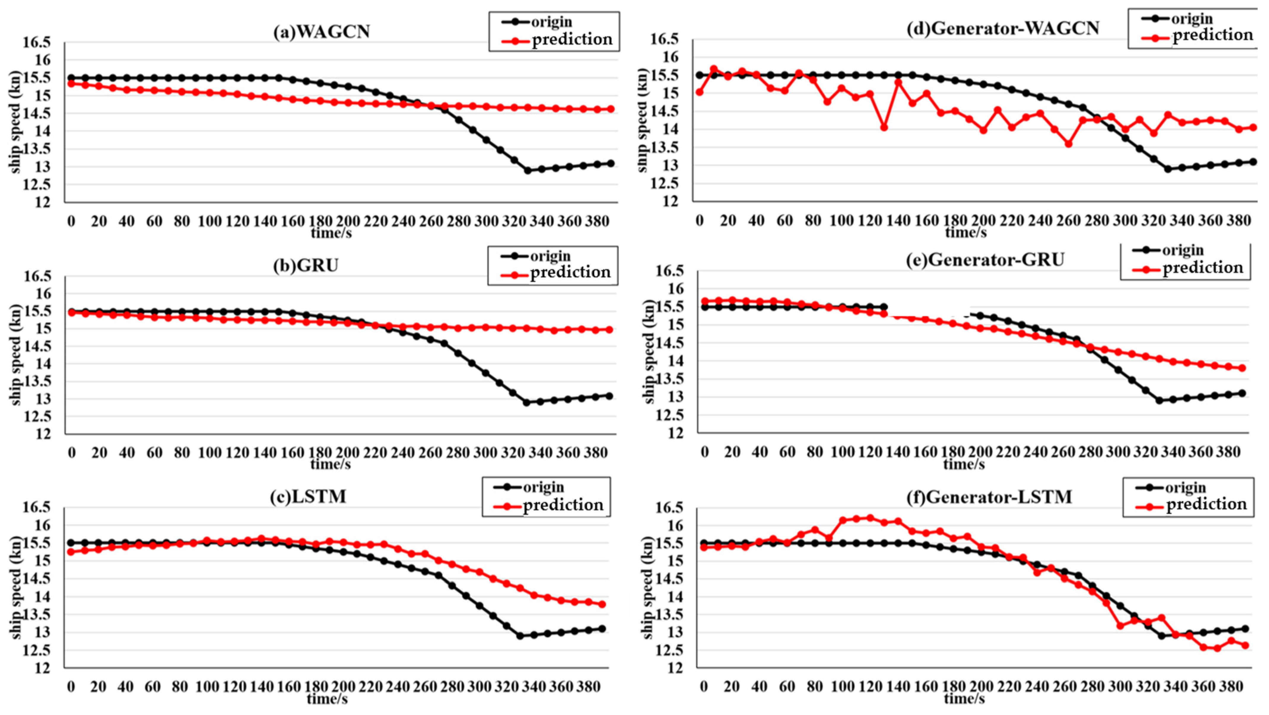
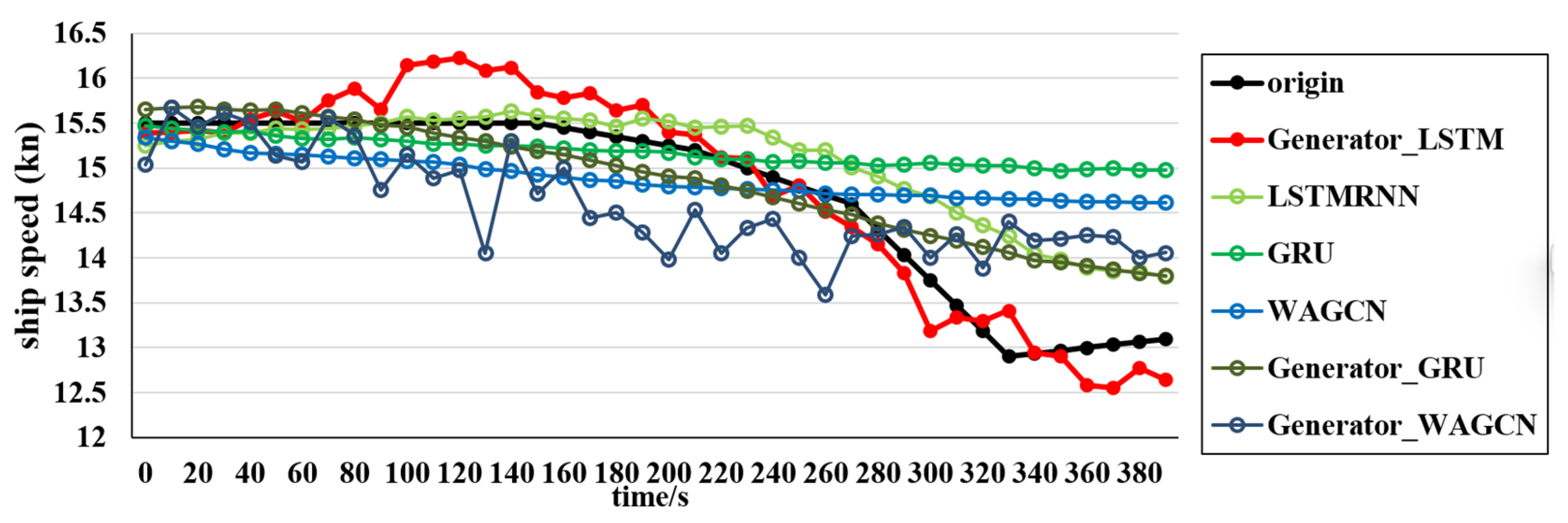
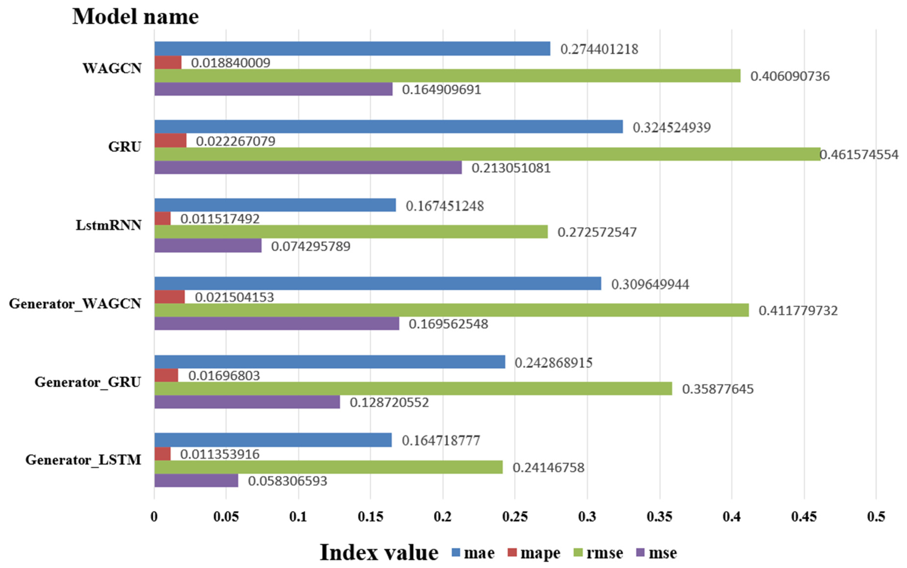
The experimental scenarios selected six types of ships, namely, container ships, oil tankers, bulk carriers, passenger ships, fishing boats, and dredgers; these can represent the ship scenarios within a certain range. The experimental comparison models include the LSTM, GRU, WAGCN, GAN–GRU, and GAN–WAGCN. Meanwhile, the benchmark tests of the target model GAN–LSTM on Transformer and GNN are included, and have certain substantive significance for the experimental verification. The comparison of the experimental index results for the six types of ships shows that GAN–LSTM has the best effectiveness in predicting ship speed. However, for the purpose of a more in-depth and critical discussion of the experimental results, it encompasses three aspects: limitations, error analysis, and practical significance. The following is a detailed elaboration of these dimensions.

4.1.1. Limitations

(1)

Discussion relating to the limitations of GAN–LSTM in predicting ship speed

In terms of data quality and quantity, the performance of the GAN–LSTM model usually depends on the quality and diversity of the training data. If the data contain noise, or are incomplete or biased, the generated prediction results may not be accurate. In the application of ship-speed prediction, collecting complete and accurate historical data is a challenge, especially due to the influence of factors such as having different types of ships, different routes, and weather conditions. A GAN–LSTM usually requires a large amount of historical data to train the model. For certain specific areas or special types of ships, it may be difficult to collect sufficient training data, which limits the performance of the model.

In terms of the complexity of model training, a GAN–LSTM requires the training of both the generator and the discriminator simultaneously, and the LSTM part also needs to handle long-term series data. This may lead to the model training process becoming extremely complex, requiring a large amount of computing resources and time for convergence. The generator in a GAN may experience pattern collapse; that is, the generated prediction results might lack diversity, resulting in the model’s inability to accurately capture the complex changes in ship speed, especially when ships are affected by various factors such as weather and sea conditions. Both the GAN and the LSTM themselves have many hyperparameters. The selection of these parameters will affect the performance of the model, and the parameter tuning process requires a large number of experiments. If the model is overly dependent on the training data, it may lead to overfitting, that is, performing poorly on new data. Especially in the prediction of ship speed, the different navigation conditions of ships may lead to gaps between the training data and the actual scenarios, which will affect the generalization ability of the model.

In addition, the speed of a ship is not only affected by historical speed data, but also by many external environmental factors, such as wind speed, ocean currents, weather, and tides [34]. Although a GAN–LSTM can capture certain patterns of ship speed through historical data, it is difficult for it to directly simulate these complex external factors, resulting in limitations to its prediction accuracy.

(2)

Discussion relating to the respective limitations of the remaining experimental models compared as to ship-speed prediction

As to the limitations of an LSTM, when dealing with long-term series data, although the LSTM represents an improvement, compared to traditional RNN, with respect to extremely long series of data, it may encounter problems such as vanishing or exploding gradients, resulting in a decline in its ability to capture long-term dependencies. The computational overhead of an LSTM is relatively high, especially when dealing with complex time-series data, which may reduce the real-time performance of the model. This is a limitation for application scenarios with high real-time requirements, such as ship-speed prediction [35].

As to the limitations of a GRU, the GRU performs slightly worse, relative to the LSTM, when modeling long-term and short-term dependencies. Although it has fewer parameters and higher computational efficiency, when capturing very long-term dependencies, the GRU performs worse, relative to the LSTM. The structure of the GRU is simpler than that of the LSTM, which also means that it is not as flexible as an LSTM when dealing with complex time-series data, especially under complex navigation conditions.

As to the limitations of a WAGCN, the WAGCN is a graph convolutional network, and is usually used to handle graph-structured data. In the context of ship-speed prediction, although it can effectively handle information with graph structures, if the task data do not have a clear graph structure, the WAGCN cannot function effectively. A WAGCN requires that the input data have a good graph-based informational structure, or that the relationships between ships needed to be modeled, which would increase the complexity of data processing and the cost of preprocessing.

As to the limitations of a GAN–GRU, similar to a GAN–LSTM, the GAN–GRU also faces the problem of generator pattern collapse, which affects the accuracy of the model. The GRU has fewer parameters compared to an LSTM, but its ability to handle long-term series is poor and it cannot effectively capture long-term dependencies in the changes of ship speed.

As to the limitations of a GAN–WAGCN, the GAN–WAGCN combines the advantages of graph convolution and Generative Adversarial Networks, but is also limited to graph-structured data. If there is no clear graph structure of the relationships between ships, it would be difficult to model, and the effectiveness of the model would be affected. A GAN–WAGCN faces a training instability problem similar to those of other GAN models and requires a good training strategy to avoid the problems of generator pattern collapse and the inability of the discriminator to be effectively trained.

(3)

Discussion of the limitations of the benchmark tests for the GAN–LSTM, the Transformer and GNN

The discussion and analysis of the limitations of a GAN–LSTM have been elaborated specifically in “(1) Discussion on the limitations of a GAN–LSTM in predicting ship speed” in this section and will not be repeated here.

The limitations of Transformer are mainly manifested in the following four aspects:

High memory consumption occurs when processing long sequences. Although Transformer is more efficient than are the RNN and LSTM when dealing with long sequences, its self-attention mechanism requires calculating the interaction information for all input sequences, which leads to high computational and memory overhead. For particularly long time series, the problem of low computational efficiency may be faced.

Transformer has a strong dependence on data quality. The Transformer model performs very well on high-quality and large-scale data. However, if the data quality is poor or the data volume is insufficient, Transformer may not achieve the expected effect, and this may even lead to overfitting due to the instability of the training data [36].

The lack of time-dependent modeling makes it difficult to handle the sequential nature of time series. Although the self-attention mechanism of Transformer can capture the dependencies at long distances in the sequence, it itself lacks an inherent mechanism for handling temporal order, which makes it less direct and effective than an LSTM when dealing with tasks that strictly rely on temporal order, such as ship-speed prediction.

Real-time prediction of delay proves difficult. Since Transformer needs to perform global calculations on the entire sequence when calculating self-attention, it will encounter computational bottlenecks in real-time or low-latency prediction tasks. Especially in application scenarios that require rapid response, Transformer cannot complete the prediction in a timely manner.

The limitations of GNN are mainly manifested in the following four aspects:

The construction of graph data is complex and the construction of graph structure is difficult. GNN mainly relies on graph structures to represent the relationships between data points. For ship-speed prediction, constructing an appropriate graph structure can be very complex, especially when the relationships between data are relatively implicit or difficult to model clearly.

It is difficult to capture global dependencies in the balance between local information and global information. Although GNN can model the relationships between local nodes well, it is not as direct and effective as an RNN or LSTM when dealing with long-term global dependencies. Ship-speed prediction involves rather complex global relationships in terms of time and space, and GNN performs poorly in this aspect.

The computational complexity of graph networks is high. When graph neural networks handle large-scale graphs, the computational and memory overheads will also increase rapidly, especially when the graph structure needs to be updated frequently and complex graph convolution needs to be performed, which will lead to a decrease in the efficiency of the model in the training and inference stages [37].

It is prone to overfitting small-scale data. In the practical application of ship-speed prediction, the dataset is not particularly large. Especially in the case of missing data or a substantial amount of noise, GNN is prone to overfitting, resulting in a poor generalization ability of the model.

4.1.2. Analysis of Errors

(1)

Sources of error

The first source of error is in the AIS data quality issues. The AIS system itself may be affected by environmental factors such as weather, sea conditions, or terrain, resulting in errors or inaccuracies during data collection. For example, ships may lose signals, or signals may be interfered with, resulting in positional errors. Inaccurate position and velocity information will affect the training and prediction results of the GAN and LSTM models. In addition, AIS data usually have a time delay, especially when the vessel is far away or the signal coverage is poor. The AIS system sometimes loses data due to hardware or communication issues. The delay or absence of historical data can lead to the inability to obtain complete information during model training, which may result in the inability to accurately capture the changing trends in ship speed during the training process, thereby affecting the prediction accuracy.

The second source of error is in the dynamic environmental factors. The speed of a ship not only depends on the operation of the vessel itself, but is also affected by the marine environment. These external factors may not have been fully considered or might be difficult to quantify accurately. If these external factors are not fully modeled or reflected in the AIS data, the prediction results of the model may not accurately reflect the actual changes in ship speed.

The third source of error is in the complexity of time-series characteristics. The variations in ship speed may present complex nonlinear and periodic characteristics. Although an LSTM is suitable for processing time-series data, it may be difficult to fully capture all time-varying patterns associated with ship speed. If the LSTM model fails to fully capture these complex time-series patterns, this may lead to an increase in prediction errors, especially during long-term predictions, in which the errors will accumulate over time.

(2)

Biases of datasets

The first dataset bias is the time synchronization bias. AIS data typically contain the timestamps and positions of ships, but due to network delays, communication issues or equipment failures, the reporting times of ships may not be completely synchronized. Therefore, there may be a certain deviation between the timestamp and the actual ship speed. Time synchronization deviation can lead to the disruption of the temporal order of data, thereby affecting the learning effectiveness of the LSTM model for the time series.

The second dataset bias consists of data noise and outliers. AIS data may sometimes contain noise or outliers, which may be caused by factors such as sensor failure and signal interference. Data noise and outliers can make it difficult for the LSTM model to learn effective patterns from normal data, affecting the training effectiveness of the model.

The third dataset bias is in the nonlinear relationship between ship speed and position. The relationship between the speed of a ship and its position may be a complex nonlinear one, and the speed of a ship may be affected by factors such as waterways, traffic density, and wind speed. In AIS data, the relationship between ship speed and position is not a simple linear one, but has strong dynamic changes. An LSTM is capable of handling nonlinear relationships in a time series. However, if the nonlinear relationships in AIS data are not modeled correctly, the LSTM model may have difficulty accurately capturing the true laws of ship-speed changes.

4.1.3. Practical Significance

The first element of practical significance is that a GAN–LSTM can improve the prediction accuracy of ship-speed prediction in practical applications, enhance the robustness of the model, and achieve ship-speed optimization.

Traditional time-series prediction methods may have limitations when dealing with complex ship-speed data, especially when the data are affected by multiple factors such as the marine environment, climate change, and ship-types. By combining LSTM with a GAN, the time-series characteristics and potentially nonlinear relationships in the ship-speed data can be effectively captured. Meanwhile, training samples that are more diverse are generated through the GAN to enhance the generalization ability of the model, thereby improving the prediction accuracy. Combining the generation ability of a GAN and the time-series modeling ability of an LSTM can enhance the model’s adaptability to various forms of complex and nonlinear data. By generating synthetic samples, a GAN can expand the training dataset, especially in the case of scarce data, enhancing the robustness of the model, enabling the model to better cope with incomplete or variable data in practical applications. In addition, accurate prediction of ship speed not only helps to enhance the safety of shipping, but also plays a positive role in optimizing routes, saving fuel, and reducing shipping costs. Through more accurate ship-speed prediction, ship managers can better plan the voyage and avoid unnecessary speed fluctuations, and thereby improve operational efficiency.

The second element of practical significance is that the GAN–LSTM can achieve automated and real-time prediction in predicting ship speed in practical applications, improving shipping logistics and achieving the goal of energy conservation and emission reduction.

The GAN–LSTM model can achieve automated ship-speed prediction in shipping systems. With the advancement of self-driving ships, real-time prediction of ship speed is of great significance in aspects such as navigation control, collision avoidance, and channel selection. The GAN–LSTM model can be utilized to provide real-time speed adjustment suggestions for ships, helping crew members better cope with varying sea conditions. In the shipping and logistics industry, accurate prediction of ship speed not only helps ships better control their voyage time, but also enables logistics companies to schedule ships more efficiently, optimizing the cargo transportation process, reducing delays, and thereby enhancing overall logistics efficiency and customer satisfaction. Accurate ship-speed prediction can help shipping companies adjust the speed of a ship based on its real-time conditions, thereby optimizing fuel consumption and reducing carbon emissions. This is of positive significance for achieving the green transformation and energy conservation and emission reduction goals of the shipping industry.

Finally, deploying the ship-speed prediction model based on a GAN–LSTM in the actual maritime traffic management system has significant practical significance.

Firstly, it can enhance navigation safety, optimize the voyage range, and reduce navigation delays, thereby improving traffic flow management and strengthening the real-time response capability of the system. Accurate prediction of ship speed helps ensure that ships can navigate as planned and reduces potential safety hazards caused by excessive fluctuations in ship speed. By using the GAN–LSTM model, the real-time speed of ships can be accurately predicted, helping the maritime traffic management system to monitor and adjust the navigation routes in real time, avoiding accidents such as collisions and stranding, and ensuring navigation safety. Traditional voyage planning usually relies on historical data and preset speeds, while the GAN–LSTM model can conduct dynamic prediction in combination with real-time data. This means that shipping companies and maritime traffic management institutions can adjust routes and speeds in real time based on accurate ship-speed predictions and optimize voyages, thereby reducing delays, improving the operational efficiency of vessels, and enhancing the overall logistics operation speed. A GAN–LSTM combines the advantages of Generative Adversarial Networks and Long Short-Term Memory networks and can quickly adapt to the changes in ship-speed prediction in the unpredictable marine environment.

Secondly, it can enhance fuel efficiency and reduce emissions, improve the efficiency of resource allocation, and provide significant support for automated navigation and intelligent shipping. In maritime traffic management, the reasonable prediction of ship speed can help ships better control their speed and avoid sailing too fast or too slow. A reasonable speed can not only save fuel but also reduce carbon emissions, which is in line with the green and environmental protection goals increasingly emphasized by the modern shipping industry. With the gradual application of automation technology, the role of accurate ship-speed prediction in automated navigation is particularly crucial [38]. The ship-speed prediction based on the GAN–LSTM model can provide accurate real-time data for the automated navigation system, helping ships automatically adjust the speed and route without manual intervention to ensure the safety and efficiency of navigation.

4.2. Construction of Marine Ship Intelligence and a Self-Navigation System

With the advancement of smart vessels, the automated navigation systems on ships must handle real-time dynamic data processing, such as weather conditions, ocean currents, hull status, and more [39]. A GAN can generate ship-speed data that match these conditions, help automated systems predict ship speed in real time, and adjust the speed according to the predicted results. This is vital for the automated operation of ships, especially in the absence of human operators, where the reliability of ship-speed forecasts directly affects the safety and efficiency of navigation [40]. In the self-navigation system of intelligent ships, a GAN can combine real-time data to predict ship-speed changes, especially the ship-speed adjustments made in bad weather or complex sea conditions.

When actually deploying the GAN–LSTM model to predict the speeds of oil tankers and container ships, the computational efficiency is associated with high requirements for real-time performance, accuracy, and resource consumption [41].

(1)

In terms of training time: The GAN–LSTM model combines the advantages of a GAN and an LSTM, but at the same time requires a longer training time. Especially when it comes to complex time-series data (such as ship speed, position, etc.), the training process can be very time-consuming. Adversarial training in a GAN requires repeated iterations of the generator and discriminator, and an LSTM needs to effectively learn the long-term dependencies in the time series [42]. The datasets of oil tankers and container ships usually include multi-dimensional time-series information (such as ship speed, heading, longitude and latitude, etc.), and a large amount of computing time and resources are consumed during the training process.

(2)

In terms of the required resources: The GAN–LSTM model requires a large amount of computing resources during the training process. Since the model contains a generator, a discriminator, and an LSTM module, all of these parts require high computational power in terms of calculation [43]. In actual deployment, this high demand may limit this application under the condition of limited resources. Speed prediction for oil tankers and container ships involves a large amount of data and usually requires real-time calculation. Therefore, the computing resource requirements during training may place higher demands on hardware platforms (such as GPU, TPU) [44]. High demands for memory and computing power may lead to performance degradation when deployed on low-configuration hardware.

4.3. Collaborative Optimization of Smart Ports and Ship-Speed Prediction

With the development of the maritime industry, the research on ship-speed prediction cannot ignore the necessity of the collaborative optimization of smart ports and routes. Smart ports can leverage IoT and Big Data technologies to monitor a wide range of dynamic information both inside and outside the port in real time, including ship locations, cargo loading and unloading progress, port weather, and more [45,46]. A GAN can optimize coordination between ships and ports through real-time ship-speed prediction and navigation data generation. For example, by predicting the accurate arrival times of ships, ports can better arrange berths, scheduling, and cargo handling plans, thereby reducing port congestion and waiting times and improving port operational efficiency [47]. In addition, the ship-speed prediction not only affects the ship sailing process but also has an important impact on the port logistics chain. Therefore, precise ship-speed prediction is a key prerequisite for optimizing the port logistics chain. The logistics management system of a smart port can use the ship-speed data generated by a GAN to optimize the cargo handling efficiency of all links from the ship to the port [48,49]. By accurately predicting ship speed, the port can reasonably arrange the flow of goods and the times at which ships enter and exit the port, and adjust the equipment and personnel configuration in advance, reducing the overall logistics cost.

With the improvements in environmental protection requirements, ship energy optimization has become the key [50]. By utilizing a GAN for ship-speed prediction, ships can more precisely manage their speed to achieve minimum fuel consumption and optimal energy use. Ship speed and fuel consumption are related in a nonlinear fashion. A GAN can generate predictive models for ship speed and fuel consumption under various sea conditions and loads, assisting ships in adjusting their speed to achieve green shipping objectives and reduce carbon emissions [51].

The GAN model is essentially a complex deep learning model that lacks sufficient interpretability. This makes the model’s predictions difficult to understand and verify, especially when key decisions require transparency and interpretability (e.g., port scheduling decisions, channel optimization) [52]. In this study, GAN architectures with better stability, such as the LSTM–GAN or WAGCN–GAN, are used, which can reduce the phenomenon of training instability by improving the loss function and regularization method. Additionally, the study began with simple tasks used to train the GAN models and progressively increased the complexity of the models. The model’s capabilities are enhanced through incremental training, facilitating easier convergence [53].

Ship-speed prediction not only aims to accurately predict ship speed, but also involves the collaborative optimization of multiple objectives, such as port scheduling, channel planning, etc., some of which may conflict with each other [54,55]. In this research, according to the importance of different target data, different types of data are prioritized and weighted, and some important targets are given priority in the training process in order to balance the conflicts between different targets [56,57]. By introducing the multi-objective optimization function into the generator and discriminator, the model can not only generate ship-speed prediction but also consider many factors such as port resource utilization efficiency and channel safety.

5. Conclusions

A GAN can be used to generate a richer training dataset. In cases where traditional models have less data or unbalanced data, a GAN can be combined in certain scenarios to enhance the training process and improve the generalization ability of the model by using the data generated by a GAN. However, the combination of traditional models and GANs can lead to unstable training, high demand for computing resources, unreliable quality of generated data, complex parameter adjustment, and difficulties in model fusion, etc. An LSTM is a kind of neural network specifically used for processing time-series data (such as the change in ship speed over time), and it can capture the long-term dependencies in the time series. Compared with traditional machine learning models, an LSTM can better capture the temporal characteristics and dynamic patterns of ship speed when processing time-series data.

In this study, a GAN–LSTM model used for ship-speed prediction is proposed, one which combines a GAN network and an LSTM model. First, the algorithm takes an LSTM network as the generating network and utilizes the LSTM to capture spatiotemporal dependencies between nodes. Secondly, the complementary characteristics linked between the generative network and the discriminant network are used to eliminate the cumulative error of a single neural network over the long-term prediction process, improving the accuracy of the network in ship-speed determination. Ultimately, the Generator–LSTM model is utilized for predicting ship speed and compared with other models, using the same AIS ship-speed information, and in the same scene. The results show that the model achieves high accuracy in typical error metrics, which means that the model can more accurately predict ship speed. In addition, the performance of the Generator–LSTM model shows the superiority of this method in the task of speed prediction. This can be attributed to the Generator–LSTM model’s ability to realize the task of speed prediction by using the spatiotemporal correlations in velocity-related data. In addition, the Generator–LSTM model has a high prediction accuracy, indicating that good temporal and spatial correlation is a crucial component of a model for accurate ship-speed prediction.

This study still has some limitations, such as the limited nature of the dataset. Although we used datasets from multiple sources, these data may not fully cover all possible actual situations. Therefore, under certain specific conditions, the prediction accuracy of the model may be reduced. Secondly, there is also a limitation related to the universality of the model. The neural network (or LSTM) model used in the research performs well in certain specific scenarios, but as to situations involving extreme or uncommon situations, the robustness of the model still needs to be further verified. Furthermore, due to the limitations in computing resources, this study failed to conduct more hyperparameter optimizations or train on larger-scale datasets. Therefore, the performance of the model may not have reached its optimum level.

In future research, it is important to further investigate the performance of this model in long-term speed-prediction tasks, and research on the expression of water-traffic situational knowledge based on AIS data is an area also worthy of further study.

References

1. Goncharov, V.K.; Klementieva, N.Y. Parameterization of the propeller thrust for modelling ship braking in ice channel behind icebreaker. Transp. Saf. Environ. 2023, 5, tdac042. [Google Scholar] [CrossRef]
2. Goncharov, V.K.; Chugaeva, A.E.; Kviatkovskaia, E.S.; Zueva, E.S. Analysis of the impact of Arctic environment conditions on the psychophysical status of navigators and the safety of ice navigation. Transp. Saf. Environ. 2024, 6, tdae019. [Google Scholar] [CrossRef]
3. Korupoju, A.K.; Kapadia, V.; Vilwathilakam, A.S.; Samanta, A. Ship Collision Risk Evaluation using AIS and weather data through fuzzy logic and deep learning. Ocean. Eng. 2025, 318, 120116. [Google Scholar] [CrossRef]
4. Li, H.; Jiao, H.; Yang, Z. AIS data-driven ship trajectory prediction modelling and analysis based on machine learning and deep learning methods. Transp. Res. Part E Logist. Transp. Rev. 2023, 175, 103152. [Google Scholar] [CrossRef]
5. Klemm, J.; Niemi, A.; Torres, F.S. Predicting Ship Tracks in Waterways Using Long Short-Term Memory. In Proceedings of the 7th International Conference on Transportation Information and Safety, Halifax, NS, Canada, 23–26 September 2024. [Google Scholar] [CrossRef]
6. Aristov, N.; Li, Z.; Koch, T.; Dugundji, E.R. Elucidating US Import Supply Chain Dynamics: A Spatial-Temporal Graph Neural Network Approach. In Proceedings of the IEEE High Performance Extreme Computing Conference, Wakefield, MA, USA, 23–27 September 2024. [Google Scholar] [CrossRef]
7. Lee, G.; Kim, D.; Park, S.; Sim, S.; Liu, L.; Bae, H. Neural Bezier Interpolation with Manifold Learning for Reliable Vessel Trajectory Prediction. In Proceedings of the IEEE 6th International Conference on Cognitive Machine Intelligence, Washington, DC, USA, 28–31 October 2024. [Google Scholar] [CrossRef]
8. Pensado, E.A.; López, F.V.; Jorge, H.G.; Pinto, A.M. UAV Shore-to-Ship Parcel Delivery: Gust-Aware Trajectory Planning. IEEE Trans. Aerosp. Electron. Syst. 2024, 60, 6213–6223. [Google Scholar] [CrossRef]
9. Magalhães, A.; Estima, J.; Cardoso, A. Vessel Voyage Trajectory Extrapolation: Comparing the Performance of Kalman Filters. In Proceedings of the 2023 6th Experiment@ International Conference, Évora, Portugal, 5–7 June 2023. [Google Scholar] [CrossRef]
10. Padmavathi, A.; Parameshachari, B.D.; Fallah, M.H.; Pushpalakshmi, G.; Saranya, N.N. A Marine Traffic Pattern Prediction System Based on Graph Convolutional and Kolmogorov-Arnold Networks. In Proceedings of the International Conference on Integrated Intelligence and Communication Systems, Kalaburagi, India, 22–23 November 2024. [Google Scholar] [CrossRef]
11. Donandt, K.; Söffker, D. Incorporating Navigation Context into Inland Vessel Trajectory Prediction: A Gaussian Mixture Model and Transformer Approach. In Proceedings of the 2024 27th International Conference on Information Fusion (FUSION), Venice, Italy, 8–11 July 2024. [Google Scholar] [CrossRef]
12. Ivanovic, P.; Windmann, A.; Neumann, P. SmartShip: Data Decoding Optimization for Onboard AI Anomaly Detection. In Proceedings of the 2024 23rd International Symposium on Parallel and Distributed Computing (ISPDC), Chur, Switzerland, 8–10 July 2024. [Google Scholar] [CrossRef]
13. Sigillo, L.; Marzilli, A.; Moretti, D.; Grassucci, E.; Greco, C.; Comminiello, D. Sailing the Seaformer: A Transformer-Based Model for Vessel Route Forecasting. In Proceedings of the 2023 IEEE 33rd International Workshop on Machine Learning for Signal Processing (MLSP), Rome, Italy, 17–20 September 2023. [Google Scholar] [CrossRef]
14. Gülsoylu, E.; Koch, P.; Yıldız, M.; Constapel, M.; Kelm, A.P. Image and AIS Data Fusion Technique for Maritime Computer Vision Applications. In Proceedings of the IEEE/CVF Winter Conference on Applications of Computer Vision Workshops, Waikoloa, HI, USA, 1–6 January 2024. [Google Scholar] [CrossRef]
15. Nitish, R.; Prabhat, K.; Divyanshi, G. Predicting Vessel Speed Using Ensemble MLR and RF Models on AIS Data. Def. Sci. Inf. Doc. Cent. 2025, 75, 250–256. [Google Scholar] [CrossRef]
16. Oleg, T.; Danila, E.; Alex, T. A benchmark study on ship speed prediction models in arctic conditions: Machine learning, process-based and hybrid approaches. Ocean. Eng. 2024, 311, 118884. [Google Scholar] [CrossRef]
17. Pappagallo, A.; Ortame, F.; Massacci, G.; Sisti, F.; Pugliese, F. Deep Learning for the Classification of Ports in Maritime Transport Statistics via AIS Data; Lecture Notes in Computer Science; Springer: Cham, Switherland, 2025; pp. 318–332. [Google Scholar] [CrossRef]
18. Kumar, R.H.; Ramanarayanan, C.P.; Bharath, R. Machine Learning Based Automated Process for Predicting the Anomaly in AIS Data; Lecture Notes on Data Engineering and Communications Technologies; Springer: Singapore, 2023; pp. 303–314. [Google Scholar] [CrossRef]
19. Marta, S.; Ireneusz, C. VAR vs XGBoost: Performance of both models in AIS data reconstruction. Procedia Comput. Sci. 2024, 246, 5084–5093. [Google Scholar] [CrossRef]
20. Xian, J.; Li, Z.; Wu, H. Novel Polarization Construction Method and Synchronization Algorithm for Underwater Acoustic Channel Under T-Distribution Noise Environment. J. Mar. Sci. Eng. 2025, 13, 362. [Google Scholar] [CrossRef]
21. Chen, X.; Hu, R.; Luo, K.; Wu, H.; Biancardo, S.A.; Zheng, Y.; Xian, J. Intelligent Ship route planning via an A* search model enhanced double-deep Q-Network. Ocean. Eng. 2025, 327, 120956. [Google Scholar] [CrossRef]
22. Ourc, M.F.; Altan, Y.C. Deep learning for risky encounter prediction: Leveraging LSTM networks and AIS data. In Advances in the Collision and Grounding of Ships and Offshore Structures; Taylor & Francis: Abingdon, UK, 2023; pp. 83–89. [Google Scholar] [CrossRef]
23. Shin, G.-H.; Yang, H. Vessel trajectory prediction in harbors: A deep learning approach with maritime-based data preprocessing and Berthing Side Integration. Ocean. Eng. 2025, 316, 119908. [Google Scholar] [CrossRef]
24. Yang, Y.; Liu, Y.; Li, G.; Zhang, Z.; Liu, Y. Harnessing the power of Machine learning for AIS Data-Driven maritime Research: A comprehensive review. Transp. Res. Part E Logist. Transp. Rev. 2024, 183, 103426. [Google Scholar] [CrossRef]
25. Mehri, S.; Alesheikh, A.A.; Basiri, A. A context-aware approach for vessels’ trajectory prediction. Ocean. Eng. 2023, 282, 114916. [Google Scholar] [CrossRef]
26. Liao, W.; Wu, Y.; Zhou, P.; Wang, H.; Yu, W.; Zhang, C.; Luo, C. Dynamic navigation: Integrating GL-STGCNN and MPC for collision avoidance with future Awareness. Ocean Eng. 2024, 309 Pt 1, 118416. [Google Scholar] [CrossRef]
27. Xian, J.; Ma, J.; Chen, X. Robust and Precise Drowning Target Localization under Dual-parameters Uncertainty. Reg. Stud. Mar. Sci. 2025, 85, 104131. [Google Scholar] [CrossRef]
28. Waltz, M.; Paulig, N.; Okhrin, O. 2-level reinforcement learning for ships on inland waterways: Path planning and following. Expert Syst. Appl. 2025, 274, 126933. [Google Scholar] [CrossRef]
29. Alam, M.M.; Spadon, G.; Etemad, M.; Torgo, L.; Milios, E. Enhancing short-term vessel trajectory prediction with clustering for heterogeneous and multi-modal movement patterns. Ocean. Eng. 2024, 308, 118303. [Google Scholar] [CrossRef]
30. Li, Y.; Liang, M.; Li, H.; Yang, Z.; Du, L.; Chen, Z. Deep learning-powered vessel traffic flow prediction with spatial-temporal attributes and similarity grouping. Eng. Appl. Artif. Intell. 2023, 126 Pt B, 107012. [Google Scholar] [CrossRef]
31. Chen, X.; Wu, S.; Shi, C.; Huang, Y.; Yang, Y.; Ke, R. Sensing Data Supported Traffic Flow Prediction via Denoising Schemes and ANN: A Comparison. IEEE Sens. J. 2020, 20, 14317–14328. [Google Scholar] [CrossRef]
32. Chen, X.; Ling, J.; Yang, Y.; Zheng, H.; Xiong, P.; Postolache, O.; Xiong, Y. Ship Trajectory Reconstruction from AIS Sensory Data via Data Quality Control and Prediction. Math. Probl. Eng. 2020, 2020, 1–9. [Google Scholar] [CrossRef]
33. Peel, G.J.; Gedikli, E.D.; Hendrikse, H. Navigating Arctic Waters: A Summary of Ship Activities and Ice-Ship Interactions in Alaskan Waters. In Proceedings of the International Conference on Port and Ocean Engineering Under Arctic Conditions, Glasgow, UK, 12–16 June 2023. [Google Scholar]
34. Chen, X.; Wei, C.; Xin, Z.; Zhao, J.; Xian, J. Ship Detection under Low-Visibility Weather Interference via an Ensemble Generative Adversarial Network. J. Mar. Sci. Eng. 2023, 11, 2065. [Google Scholar] [CrossRef]
35. Wang, D.; Jing, Y. Ship collision risk analysis in port waters integrating GRA algorithm and BPNN. Transp. Saf. Environ. 2025, 7, tdaf012. [Google Scholar] [CrossRef]
36. Liu, X.; Qiu, L.; Fang, Y.; Wang, K.; Li, Y.; Rodríguez, J. Event-Driven Based Reinforcement Learning Predictive Controller Design for Three-Phase NPC Converters Using Online Approximators. IEEE Trans. Power Electron. 2025, 40, 4914–4926. [Google Scholar] [CrossRef]
37. Gao, X.; Dai, W.; Yu, L.; Yu, Q. Study on factors contributing to severity of ship collision accidents in the Yangtze River estuary. Transp. Saf. Environ. 2024, 6, tdae014. [Google Scholar] [CrossRef]
38. Liu, X.; Qiu, L.; Fang, Y.; Wang, K.; Li, Y.; Rodríguez, J. Combining Data-Driven and Event-Driven for Online Learning Predictive Control in Power Converters. IEEE Trans. Power Electron. 2025, 40, 563–573. [Google Scholar] [CrossRef]
39. Huu, K.D. A Speed Prediction Model Using A HIL Simulator and Neural Network for Cargo Ships. In Proceedings of the International Russian Smart Industry Conference, Sochi, Russia, 25–29 March 2024. [Google Scholar] [CrossRef]
40. Zhu, Q.; Xi, Y.; Weng, J.; Han, B.; Hu, S.; Ge, Y.-E. Intelligent ship collision avoidance in maritime field: A bibliometric and systematic review. Expert Syst. Appl. 2024, 252 Pt A, 124148. [Google Scholar] [CrossRef]
41. Chen, J.; Zhuang, C.; Shi, J.; Jiang, H.; Xu, J.; Liu, J. Risk factors extraction and analysis of Chinese ship collision accidents based on knowledge graph. Ocean Eng. 2025, 322, 120536. [Google Scholar] [CrossRef]
42. Karachalios, T.; Moschos, P.N.; Fanariotis, A.; Orphanoudakis, T.; Leligou, H.-C. Integration of AIS Data for Efficient Drone Navigation in Maritime Real-Time Ship Inspection Missions. In Proceedings of the IEEE/SICE International Symposium on System Integration, Munich, Germany, 21–24 January 2025. [Google Scholar] [CrossRef]
43. Dai, Y.; He, Y.; Zhao, X.; Xu, K. Testing method of autonomous navigation systems for ships based on virtual-reality integration scenarios. Ocean Eng. 2024, 309 Pt 2, 118597. [Google Scholar] [CrossRef]
44. Han, Z.; Wu, D.; Zhang, J.; Huan, T.; Han, Q.-L.; Zhang, M. COLREGs-Adaptive trajectory planning and decision-making in maritime autonomous surface ships. Ocean Eng. 2024, 312 Pt 3, 119308. [Google Scholar] [CrossRef]
45. Purcell, E.; Nejad, A.R.; Böhm, A.; Sapp, L.; Lund, J.; Von Bock und Polach, F.; Nickerson, B.M.; Bekker, A.; Gilges, M.; Saleh, A.; et al. On Methodology for a digital twin of ship propulsion under harsh environmental conditions. In Proceedings of the International Conference on Offshore Mechanics and Arctic Engineering, Singapore, 9–14 June 2024. [Google Scholar] [CrossRef]
46. Zhen, R.; Lv, P.; Shi, Z.; Chen, G. A novel fuzzy multi-factor navigational risk assessment method for ship route optimization in costal offshore wind farm waters. Ocean. Coast. Manag. 2023, 232, 106428. [Google Scholar] [CrossRef]
47. Zhao, L.; Song, Y.; Xiong, J.; Xu, J.; Li, D.; Liu, F.; Shen, T. A time-delay neural network for ship-radiated noise recognition based on residual block and attention mechanism. Digit. Signal Process. 2024, 149, 104504. [Google Scholar] [CrossRef]
48. Hummel, H.I.; van der Mei, R.; Bhulai, S. A survey on machine learning in ship radiated noise. Ocean Eng. 2024, 298, 117252. [Google Scholar] [CrossRef]
49. Acharya, D.; Farazi, M.; Rolland, V.; Petersson, L.; Rosebrock, U.; Smith, D.; Ford, J.; Wang, D.; Tuck, G.N.; Little, L.R.; et al. Towards automatic anomaly detection in fisheries using electronic monitoring and automatic identification system. Fish. Res. 2024, 272, 106939. [Google Scholar] [CrossRef]
50. Meng, X.; Li, H.; Zhang, W.; Zhou, X.-Y.; Yang, X. Analyzing risk influencing factors of ship collision accidents: A data-driven Bayesian network model integrating physical knowledge. Ocean. Coast. Manag. 2024, 256, 107311. [Google Scholar] [CrossRef]
51. Park, M.-H.; Lee, C.-H.; Hur, J.-J.; Lee, W.-J. Prediction of fuel consumption and shaft torque using machine learning and analysis of engine curve diagrams. Meas. J. Int. Meas. Confed. 2025, 248, 116984. [Google Scholar] [CrossRef]
52. Xian, J.; Ma, J.; Mei, X.; Wu, H.; Saeed, N.; Han, D.; Marino, M.D.; Li, K.-C. Robust Coarse-to-fine 3D-Target-Localization Algorithm for Underwater-IoT-Based Networks: Design and Performance Evaluation Under Uncertain Multi-Parameter. IEEE Internet Things J. 2025, 104131. [Google Scholar] [CrossRef]
53. Umar, Z.; Junaid, K.; Eunkyu, L.; Sajjad, H.; Salim, B.A.; Yahya, A.R.; Kyungsup, K. An Efficient Long Short-Term Memory and Gated Recurrent Unit Based Smart Vessel Trajectory Prediction Using Automatic Identification System Data. Comput. Mater. Contin. 2024, 81, 1789–1808. [Google Scholar] [CrossRef]
54. Wang, W.; Liu, B.; Tian, Q.; Xu, X.; Peng, Y.; Peng, S. Predicting dust pollution from dry bulk ports in coastal cities: A hybrid approach based on data decomposition and deep learning. Environ. Pollut. 2024, 350, 124053. [Google Scholar] [CrossRef]
55. Lin, C.; Zhen, R.; Tong, Y.; Yang, S.; Chen, S. Regional ship collision risk prediction: An approach based on encoder-decoder LSTM neural network model. Ocean Eng. 2024, 296, 117019. [Google Scholar] [CrossRef]
56. Xian, J.; Wu, H.; Mei, X.; Zhang, Y.; Chen, X.; Zhang, Q.; Liang, L. Novel energy-efficient opportunistic routing protocol for marine wireless sensor networks based on compressed sensing and power contro. J. Ocean. Univ. China 2022, 21, 1504–1516. [Google Scholar] [CrossRef]
57. Watanabe, E.; Samanta, S.; Kowatari, K.; Shibasaki, R. On Vessel Schedule Delay and Its Recoveries in Liner Services Using AIS Data. In Proceedings of the IEEE International Conference on Big Data, Washington, DC, USA, 15–18 December 2024. [Google Scholar] [CrossRef]
Figure 1. Data preprocessing flow chart.
Jmse 13 01045 g001
Figure 2. Basic block diagram.
Jmse 13 01045 g002
Figure 3. GAN network architecture diagram.
Jmse 13 01045 g003
Figure 4. LSTM: basic structure diagram.
Jmse 13 01045 g004
Figure 5. The container ship.
Jmse 13 01045 g005
Figure 6. The oil tanker.
Jmse 13 01045 g006
Figure 7. The bulk cargo ship.
Jmse 13 01045 g007
Figure 8. The passenger ship.
Jmse 13 01045 g008
Figure 9. The fishing vessel.
Jmse 13 01045 g009
Figure 10. The sand dredger.
Jmse 13 01045 g010
Figure 11. Comparison of model ship-speed prediction results in the tanker scenario.
Jmse 13 01045 g011
Figure 12. Comparison of overall prediction results of 6 models under container ship scenario.
Jmse 13 01045 g012
Figure 13. Comparison of the model indicators in the container-ship scenario.
Jmse 13 01045 g013
Figure 14. Comparison of model ship speed prediction results in tanker scenario.
Jmse 13 01045 g014
Figure 15. The overview of the prediction results from the six models in the tanker scenario.
Jmse 13 01045 g015
Figure 16. Comparison of model indices in the tanker scenario.
Jmse 13 01045 g016