NMPC-Based 3D Path Tracking of a Bioinspired Foot-Wing Amphibious Robot

Abstract

To achieve accurate 3D path tracking of a foot-wing hybrid-driven amphibious biomimetic robot under periodically varying forces, this study analyzes the periodic propulsion forces generated by the flapping motion of the robot’s feet and wings, along with the nonlinear hydrodynamic effects during underwater motion. To simplify the resulting complex force expressions, the scaling function averaging method is applied. Consequently, an accurate six-degree-of-freedom (6-DOF) dynamic model is established, in which the characteristic parameters of foot-wing flapping are adopted as control inputs. Based on this dynamic model, a nonlinear state-space representation of the robot’s underwater motion is constructed. In this formulation, 3D path tracking—derived from the Line-of-Sight (LOS) guidance method—and attitude stabilization are jointly defined as control objectives. To this end, a nonlinear model predictive control (NMPC) algorithm is employed to compute optimal control inputs, as it effectively addresses the challenges of strong nonlinearity, coupling effects, and multi-objective optimization. Finally, simulation experiments are conducted to validate the proposed control strategy. The results demonstrate that the robot is capable of accurately following the desired path. Furthermore, compared with conventional PID control, the NMPC approach significantly improves tracking stability and enhances the overall motion performance.

1. Introduction

In recent years, the growing demand for underwater operations—such as marine resource exploration, environmental monitoring, underwater archaeology, defense reconnaissance, and search and rescue—has driven the development of advanced marine equipment. Among these, underwater robots play a vital role in both underwater exploration and resource acquisition. However, conventional underwater robots face significant limitations when applied to biological data collection, military reconnaissance, and operations in complex terrains [1]. To overcome these challenges, biomimetic underwater robots have been developed by mimicking the morphology and locomotion mechanisms of aquatic organisms. Compared to traditional propulsion systems, biomimetic propulsion offers higher efficiency, enhanced maneuverability, and reduced hydrodynamic disturbance [2]. Equipped with multi-degree-of-freedom biomimetic actuators, these robots demonstrate highly flexible motion, which makes them well-suited for complex and dynamic underwater environments. Furthermore, their resemblance to marine life, combined with low-disturbance propulsion, enables effective observation and tracking of aquatic animals. These features also contribute to improved performance in specific military reconnaissance tasks.

The motion control of biomimetic underwater robots serves two primary purposes: replicating the locomotion patterns of aquatic organisms and ensuring navigation along a designated trajectory or at a specified speed. These tasks can be classified into five key aspects: direction, depth, speed, stability, and trajectory control [3]. Trajectory control functions as a closed-loop system that integrates direction and depth control to enable basic path tracking. The inclusion of speed control further enhances tracking accuracy by minimizing position errors. In addition, stability control plays a vital role in underwater locomotion. It is typically achieved by adjusting the robot’s pitch and roll angles to maintain dynamic equilibrium during motion.

Various control strategies have been applied to underwater robotic motion control, including proportional-integral-derivative (PID) control [4], linear quadratic regulators (LQR) [5], sliding mode control (SMC) [6], model predictive control (MPC) [7], fuzzy logic control (FLC) [8], and neural network-based control methods [9]. These approaches have demonstrated reliable performance in terms of both control accuracy and system stability. To address the path tracking problem of underactuated surface vessels, So-Ryeok Oh et al. [10] developed a three-degree-of-freedom (3-DOF) dynamic model for an unmanned surface vehicle within an MPC framework. Line-of-Sight (LOS) guidance was integrated, and the optimal control inputs were computed using quadratic programming (QP). For planar underwater robotic motion, Shen et al. [11] derived nonlinear state-space equations and applied linear feedback techniques to compute the required propulsion forces. Path tracking inputs were then generated through MPC-based optimization. Simulation results confirmed the effectiveness of this method. In another study, Wang et al. [12] developed a two-dimensional dynamic model of a biomimetic robotic fish driven by a single joint. The model considered flow field disturbances, and a hybrid control strategy combining MPC and PID was implemented in a still-water environment. This approach enabled the robot to effectively reach target points. Yang et al. [13] proposed a two-layer control architecture that integrated robust model predictive control (RMPC) with central pattern generators (CPG). This method significantly improved trajectory tracking accuracy and enhanced the closed-loop stability of biomimetic underwater robots operating in complex disturbance environments.

The bipedal amphibious biomimetic robot investigated in this study integrates terrestrial walking mechanisms with flapping wing technology. Its multi-degree-of-freedom wing-foot structure enables three primary modes of locomotion: walking on land, crawling on the seabed, and swimming underwater. During underwater swimming, propulsion is generated by the flapping motion of the foot-wings. This driving force is regulated by adjusting the characteristic parameters of the limb joints, thereby controlling both the posture and position of the robot. The robot’s underwater dynamics are subject to strong coupling and various nonlinear hydrodynamic effects, which significantly complicate motion control. Moreover, the generated propulsion force is inherently periodic and time-varying, posing challenges to system stability. Since the propulsion acts in three dimensions, the direction and magnitude of the overall force vector change dynamically as the limb parameters are modified. These variations further influence the robot’s balance and posture during underwater movement.

Considering the three aforementioned issues and the task requirements for 3D path tracking, this study first employs blade element theory to accurately calculate the propulsion force generated by the flapping motion of the foot-wings. Nonlinear hydrodynamic effects, including viscous forces and added mass, are incorporated to establish a precise six-degree-of-freedom (6-DOF) dynamic model of the robot. To simplify the periodic characteristics of the propulsion force, a scale function averaging method is applied, which facilitates subsequent controller design. The path tracking objective, based on LOS guidance, along with the robot’s balance parameters, is then embedded into the state-space model. An NMPC algorithm is subsequently utilized to perform optimization and determine the optimal control inputs. Simulation results demonstrate that the proposed strategy enables accurate path tracking while maintaining stable attitude control throughout 3D underwater motion.

2. Overall Control Scheme

The foot-wing hybrid amphibious robot employs winged feet as its primary propulsion mechanism. By adjusting key parameters—such as the amplitude, frequency, phase difference, and equilibrium position of the foot-wing joints—the flapping-generated propulsion force can be modulated, thereby influencing the robot’s buoyancy and stability during underwater motion [14]. According to the findings in [14], multiple CFD simulations were conducted to identify the parameters affecting the forces and moments generated by fin flapping. The amplitude, frequency, and phase of the joints primarily influence thrust, while the equilibrium position mainly affects lift with minimal impact on thrust. Based on this analysis, the robot’s horizontal and vertical motions can be controlled independently.

The robot generates three-dimensional propulsion forces. During yaw maneuvers, differential thrust between the left and right foot-wings is applied. However, such adjustments often disrupt the force balance in other directions. Excessive yaw angles or prolonged yawing may result in the accumulation of rolling moments, which can destabilize the robot or even lead to capsizing. Therefore, it is essential to incorporate attitude stabilization control into the path-tracking system to ensure motion stability and overall balance during 3D navigation.

In previous studies, Chen’s work [15] did not consider the coupling effects among multiple degrees of freedom in underwater robot motion. The use of conventional PID control limited the system to single-variable regulation, making it ineffective for addressing multivariable coupling challenges during underwater operations. Moreover, the neural network-based PID controller demonstrated limited precision and robustness, falling short of the requirements for complex and dynamic underwater environments. In Yang’s study [13], a transformation function was introduced to connect RMPC with the CPG layer by mapping the forces and torques generated by RMPC to characteristic parameters—such as frequency and phase—within the CPG network. However, the design of this mapping function is complex and requires additional consideration of nonlinear phenomena, including saturation and dead zones. These factors increase implementation difficulty and reduce engineering practicality.

Given the objective of achieving both accurate trajectory tracking and stable posture control, conventional single-objective methods such as PID are insufficient. These approaches lack the ability to coordinate multiple control objectives simultaneously. In addition, the mapping and inverse mapping functions designed in Yang’s work are highly complex, creating significant challenges for real-world implementation. To address these limitations, this study proposes a direct derivation of the mapping relationship between flapping-fin parameters and the resulting forces and moments. An optimization-based control algorithm is then employed to compute these parameters directly. This approach simplifies the control pipeline and improves both real-time performance and engineering applicability.

Since the equilibrium position of the joints significantly influences the lift generated by the foot-wings while having only a limited effect on thrust, the 3D path tracking task is decomposed into horizontal trajectory tracking and vertical depth regulation. The implementation framework of the proposed path-tracking controller is presented in Figure 1.

In the horizontal plane, path tracking is achieved by generating differential thrust between the left and right foot-wings. However, this approach can introduce force imbalances in other directions, thereby requiring the integration of attitude stabilization control into the horizontal motion controller. This results in a multi-objective control problem that demands both accurate horizontal tracking and stable body posture. Given the strong coupling and high nonlinearity of the robot’s underwater dynamics, a combined LOS and NMPC strategy is adopted for the design of the horizontal motion controller, based on a comprehensive analysis of system characteristics.

For depth control, the objective is to guide the robot to reach and maintain a specified depth. To this end, a simple LOS–PID strategy is employed for the design of the snorkeling motion controller. The desired pitch angle for vertical motion is calculated using the LOS method, and the robot is steered toward this angle by adjusting the equilibrium positions of the limb joints through PID control.

Finally, the 3D desired path, together with the robot’s actual position and attitude angles, is provided as input to the control system. The horizontal and snorkeling motion controllers subsequently generate the corresponding control inputs for the robot model, thereby enabling accurate tracking of the desired 3D trajectory.

3. Dynamics Modeling of the Flapping-Based Underwater Robot

The dynamic model provides the mathematical foundation for the design of the robot’s control system. Due to the pronounced nonlinearities and strong coupling effects present in the robot’s underwater hydrodynamics, an in-depth analysis of its swimming dynamics is essential for accurate modeling and effective control design.

3.1. Coordinate System Definition

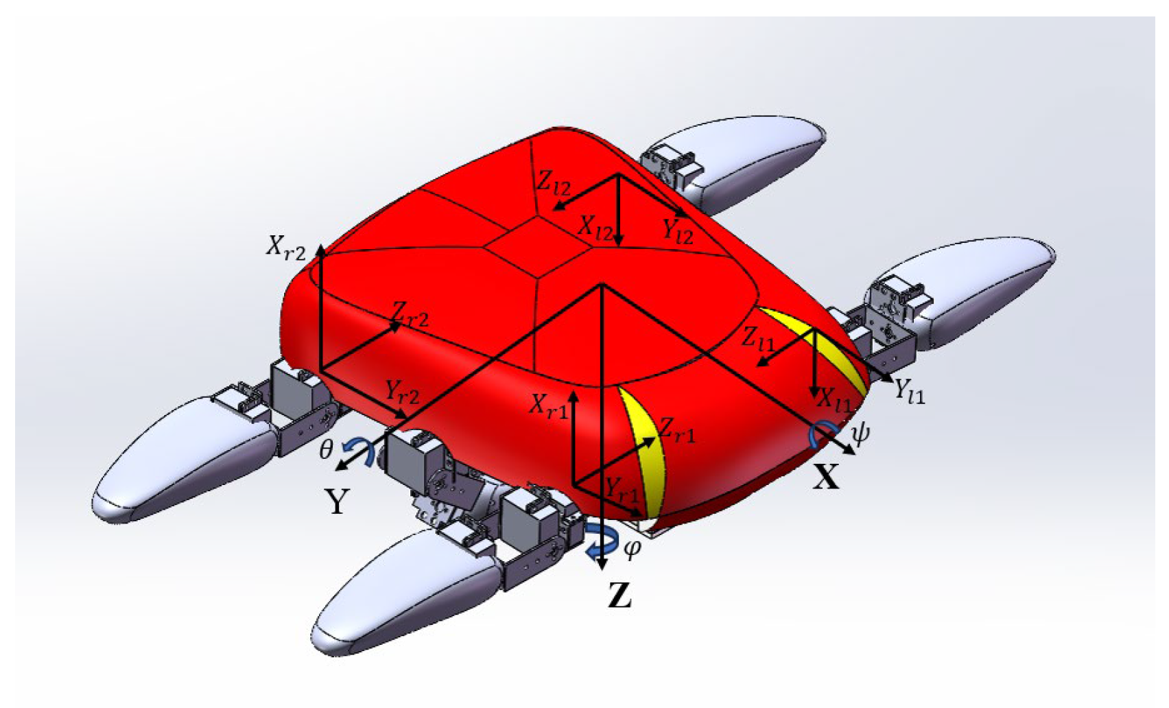
To facilitate motion analysis of the foot-wing hybrid amphibious robot, the coordinate systems shown in Figure 2 are defined in this study. When the robot is stationary, the earth-fixed coordinate system E-XYZ coincides with the body-fixed coordinate system O-XYZ, whose origin O is located at the robot’s center of mass. The positive OX-axis points forward, OY corresponds to the lateral direction, and OZ indicates the vertical motion. To compute and represent the propulsion forces generated by the four foot-wings, four local coordinate systems are established at the joints connecting the limbs to the main body. These local systems are denoted as $O_{l1}-x_{l1}{y}_{l1}{z}_{l1}$, $O_{l2}-x_{l2}{y}_{l2}{z}_{l2}$, $O_{r1}-x_{r1}{y}_{r1}{z}_{r1}$, and $O_{r2}-x_{r2}{y}_{r2}{z}_{r2}$, corresponding to the first and second foot-wings on the left and right sides, respectively. The origin of each local coordinate system is placed at the attachment point between the respective limb and the robot’s torso. Among the coordinate systems defined above, only the earth-fixed frame E-XYZ remains constant, while the body-fixed frame O-XYZ and the four local frames vary with the robot’s pose, as they are rigidly attached to the body.

In 3D space, the robot’s orientation relative to the earth-fixed coordinate system is described by three Euler angles: $\theta$, $\psi$, and $\phi$, which correspond to pitch, roll, and yaw, respectively. The robot’s motion state is defined as the vector [u, v, w, p, q, r], where u, v, and w represent surge, sway, and heave velocities, and p, q, and r represent roll, pitch, and yaw angular velocities.

3.2. Flapping-Based Swimming Dynamics Modeling

During underwater swimming, the robot is subjected to nonlinear hydrodynamic forces, including added mass effects and viscous drag. In addition, the flapping motion of each foot-wing significantly influences the overall dynamic behavior of the system. To facilitate controller design and reduce computational complexity, this study adopts a simplified dynamic model proposed in [16] to represent the robot’s swimming dynamics. This choice is based on the similarity between the robot’s configuration and actuation method and those described in [16]. The model is formulated as follows:

$$\mathbf{F}=\mathbf{M}{\mathit{v}}^{\prime }+\mathbf{c}(\mathit{v})\mathit{v}$$

(1)

The resultant force F consists of the robot’s weight and buoyancy, the thrust generated by the flapping foot-wings, and the viscous hydrodynamic forces exerted by the surrounding fluid. The matrix M denotes the generalized mass matrix, composed of the rigid-body mass matrix ${\mathbf{M}}_{\mathbf{r}}$ and the added mass matrix ${\mathbf{M}}_f$. The Coriolis matrix $\mathbf{c}(\mathit{v})$ also consists of two components: the rigid-body Coriolis and centrifugal matrix ${\mathbf{c}}_{\mathbf{r}}\left(\mathit{v}\right)$, and the added mass Coriolis matrix ${\mathbf{c}}_{\mathbf{f}}\left(\mathit{v}\right)$. The vector $\mathit{v}$, defined as $\mathit{v}$ = [${\mathit{v}}_{\mathit{r}}^{\mathit{T}};{\mathit{w}}_{\mathit{r}}^{\mathit{T}}$], represents the spatial velocity of the robot. The expressions for the rigid-body mass matrix and Coriolis matrix are given as follows:

$${\mathrm{M}}_{\mathrm{r}}=\left[\begin{array}{cccccc}m& 0& 0& 0& 0& 0\\ 0& m& 0& 0& 0& 0\\ 0& 0& m& 0& 0& 0\\ 0& 0& 0& I_{xx}& -I_{xy}& -I_{xz}\\ 0& 0& 0& -I_{xy}& I_{yy}& -I_{yz}\\ 0& 0& 0& -I_{xz}& -I_{yz}& I_{zz}\end{array}\right]$$

(2)

$${\mathbf{c}}_{\mathbf{r}}(\mathit{v})=\left[\begin{array}{cccccc}0& 0& 0& 0& mw& -mv\\ 0& 0& 0& -mw& 0& mu\\ 0& 0& 0& mv& -mu& 0\\ 0& 0& 0& 0& -I_{yz}q-I_{xz}p+I_{zz}r& I_{yz}r+I_{xy}p-I_{yy}q\\ 0& 0& 0& I_{yz}q+I_{xz}p-I_{zz}r& 0& -I_{xz}r-I_{xy}q+I_{xx}p\\ 0& 0& 0& -I_{yz}r-I_{xy}p+I_{yy}q& I_{xz}r+I_{xy}q-I_{xx}p& 0\end{array}\right]$$

(3)

where m denotes the mass of the robot body, $I_{xx}$, $I_{yy}$, and $I_{zz}$, represent the moments of inertia about the body-fixed axes Ox, Oy, and Oz, respectively, and $I_{xy}$, $I_{xz}$, and $I_{yz}$, denote the products of inertia. Considering the robot’s low swimming speed and approximate symmetry with respect to the YOZ and XOZ planes, the added mass matrix and the added Coriolis matrix are simplified as diagonal matrices, as shown below:

$${\mathbf{M}}_f=\mathrm{diag}[-X_u;-Y_v;-Z_w;-L_p;-M_q;-N_r;]$$

(4)

where $X_u$, $Y_v$, and $Z_w$ represent the linear acceleration coefficients of the robot body, and $L_p$, $M_q$, and $N_r$ denote the angular acceleration coefficients.

$${\mathbf{c}}_{\mathbf{f}}(\mathit{v})=\left[\begin{array}{cccccc}0& 0& 0& 0& -Z_{w}w& Y_{v}v\\ 0& 0& 0& Z_{w}w& 0& -X_{u}u\\ 0& 0& 0& -Y_{v}v& X_{u}u& 0\\ 0& -Z_{w}w& Y_{v}v& 0& -N_{r}r& M_{q}q\\ Y_{v}v& 0& -X_{u}u& N_{r}r& 0& -L_{p}p\\ -Y_{v}v& X_{u}u& 0& -M_{q}q& L_{p}p& 0\end{array}\right]$$

(5)

To facilitate subsequent controller design, Equation (1) is reformulated in state-space form. The state vector is defined as $\mathit{v}$ = [u, v, w, p, q, r], and the control input vector as F = $\left[F_x,F_y,F_z,M_x,M_y,M_z\right]$.

$${\mathit{v}}^{\prime }=-{\mathbf{M}}^{-1}\mathbf{c}(\mathit{v})\mathit{v}+{\mathbf{M}}^{-1}\mathbf{F}$$

(6)

A complete physical model of the robot was constructed in the relevant software, and the values of the variables in Equations (2)–(5) were obtained through the following measurement: m = 7 kg, $S_x$ = 0.0194 ${\mathrm{m}}^2$, $S_y$ = 0.0106 ${\mathrm{m}}^2$, and $S_z$ = 0.126 ${\mathrm{m}}^2$. The remaining variables adopt the same values as reported in [17]. By substituting these parameter values into Equation (6), the resulting expression is obtained as follows:

$$\left[\begin{array}{c}{u}^{\prime }\\ v^{\prime }\\ w^{\prime }\\ p^{\prime }\\ q^{\prime }\\ r^{\prime }\end{array}\right]=\left[\begin{array}{c}0.7653wq+3.2041vr\\ -0.2389wp-0.31214ur\\ 4.1867vp-1.3067uq\\ -0.0404uw+20.1926vw-0.0003pr-0.7685qr\\ -16.032uw+0.0909vw+0.5616pr-0.0002qr\\ -9.0188uv+0.2995pq+0.0017p^2-0.0017q^2\end{array}\right]+{\mathbf{M}}^{-1}\left[\begin{array}{c}{F}_x\\ F_y\\ F_z\\ M_x\\ M_y\\ M_z\end{array}\right]$$

(7)

3.3. Gravity and Buoyancy

When the robot is stationary underwater, it exhibits neutral buoyancy, meaning that its weight is equal to the buoyant force. However, the center of gravity does not coincide with the center of buoyancy. To satisfy mass distribution requirements and ensure stability through a restoring buoyant moment, the center of buoyancy is typically positioned slightly above the center of gravity. The buoyant moment acting on the robot, expressed in the body-fixed coordinate system, is given by:

$${\mathbf{M}}_{\mathbf{B}}=B\left[\begin{array}{c}{z}_b\cos \theta \sin \psi -y_b\cos \theta \cos \psi \\ x_b\cos \theta \cos \psi +z_b\sin \theta \\ -x_b\cos \theta \sin \psi -y_b\sin \theta \end{array}\right]$$

(8)

Since the robot is neutrally buoyant, the net effect of gravity and buoyancy forces is neglected. In the above equation, B denotes the magnitude of the robot’s buoyant force, and $(x_b,y_b,z_b)$ represents the position vector of the center of buoyancy in the body-fixed coordinate system.

3.4. Modeling of Foot-Wing Flapping Force

The flapping motion of the robot’s foot-wings generates a three-dimensional, time-varying, and periodic propulsion force, which serves as the primary driving source for underwater locomotion. To achieve effective motion control, it is essential to accurately calculate the forces produced during flapping. Based on blade element theory, each foot-wing is discretized into multiple infinitesimal elements along the spanwise direction. For an arbitrary element iii, the lift, thrust, and added mass forces generated during flapping are calculated using the Kutta–Joukowski lift theorem. These elemental forces are then transformed into the local coordinate system defined at the foot-wing joint through a coordinate transformation. By integrating the transformed forces across all elements, the total flapping force of the foot-wing is obtained.

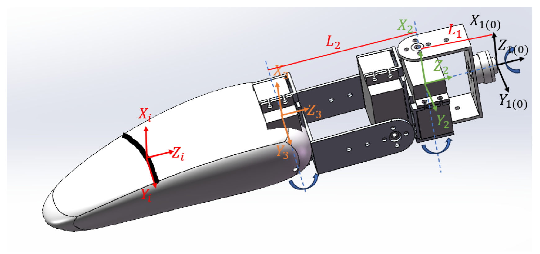
The robot’s foot-wing possesses three degrees of freedom: swing motion about the Z-axis, up-and-down flapping about the Y-axis, and forward-and-backward flapping about the X-axis. Correspondingly, a coordinate system is established for the fin, as shown in Figure 3. Coordinate system $O_0-x_0{y}_0{z}_0$ (marked in black in the figure) is established at the joint between the foot-wing and the robot body, fixed to the body with its origin at the connection point. Coordinate system $O_1-x_1{y}_1{z}_1$ (marked in black in the figure) is attached to the first joint, which performs swing motion around the Z-axis. Coordinate system $O_2-x_2{y}_2{z}_2$ (marked in green in the figure) is associated with the second joint, enabling forward-and-backward flapping around the X-axis. Coordinate system $O_3-x_3{y}_3{z}_3$ (marked in orange in the figure) is placed at the third joint, allowing up-and-down flapping about the Y-axis. In addition, a local coordinate system $O_i-x_i{y}_i{z}_i$ (marked in red in the figure) is defined at the i-th blade element of the foot-wing to facilitate force transformation. In the corresponding figure, $L_1$ denotes the Z-axis distance between coordinate systems $O_1$ and $O_2$, and $L_2$ denotes the Z-axis distance between $O_2$ and $O_3$. The motion principles and coupling relationships among the foot-wing’s degrees of freedom are detailed in [17].

The transformation matrix T between coordinate systems is defined by the three joint rotation angles $[{\phi }_1,{\phi }_2,{\phi }_3]$. Specifically, ${\phi }_1$ represents the swing angle of Joint 1 (rotation about the Z-axis), ${\phi }_2$ denotes the forward–backward flapping angle of Joint 2 (rotation about the X-axis), and ${\phi }_3$ indicates the up-and-down flapping angle of Joint 3 (rotation about the Y-axis).

$$\mathbf{T}=\left[\begin{array}{ccc}\cos {\phi }_1\cos {\phi }_3-\sin {\phi }_1\sin {\phi }_2\sin {\phi }_3& -\sin {\phi }_1\cos {\phi }_2& \cos {\phi }_1\sin {\phi }_3+\sin {\phi }_1\sin {\phi }_2\cos {\phi }_3\\ \sin {\phi }_1\cos {\phi }_3+\cos {\phi }_1\sin {\phi }_2\sin {\phi }_3& \cos {\phi }_1\cos {\phi }_2& \sin {\phi }_1\sin {\phi }_3-\cos {\phi }_1\sin {\phi }_2\cos {\phi }_3\\ -\cos {\phi }_1\sin {\phi }_3& \sin {\phi }_2& \cos {\phi }_2\cos {\phi }_3\end{array}\right]$$

(9)

Meanwhile, the flapping velocity of blade element i in the $O_0$ coordinate system can be expressed using a Jacobian transformation as ${\mathit{v}}_i^0={\mathbf{J}}_{\mathbf{i}}[{{\phi }_1}^{\prime };{{\phi }_2}^{\prime };{{\phi }_3}^{\prime }]$.

$$\begin{gathered} {\mathbf{J}}_{\mathbf{i}}=\left[\begin{array}{cc}-\sin {\phi }_1\sin {\phi }_{3}r+\cos {\phi }_1\sin {\phi }_2\cos {\phi }_{3}r+\cos {\phi }_1\sin {\phi }_2{l}_2& \sin {\phi }_1\cos {\phi }_2\cos {\phi }_{3}r+\sin {\phi }_1\cos {\phi }_2{l}_2\\ \cos {\phi }_1\sin {\phi }_{3}r+\sin {\phi }_1\sin {\phi }_2\cos {\phi }_{3}r+\sin {\phi }_1\sin {\phi }_2{l}_2& -\cos {\phi }_1\cos {\phi }_2\cos {\phi }_{3}r-\cos {\phi }_1\cos {\phi }_2{l}_2\\ 0& -\sin {\phi }_2\cos {\phi }_{3}r-\sin {\phi }_2{l}_2\end{array}\right. \\ \left.\begin{array}{c}\cos {\phi }_1\cos {\phi }_{3}r-\sin {\phi }_1\sin {\phi }_2\sin {\phi }_{3}r\\ \sin {\phi }_1\cos {\phi }_{3}r+\cos {\phi }_1\sin {\phi }_2\sin {\phi }_{3}r\\ -\cos {\phi }_2\sin {\phi }_{3}r\end{array}\right] \end{gathered}$$

(10)

During underwater motion, the robot maintains a forward velocity denoted by $U_0$. As a result, the relative velocity of the i-th foot-wing element with respect to the incoming flow, expressed in the local coordinate frame $O_1$, is the vector sum of the flapping velocity and the translational velocity of the robot. According to the Kutta–Joukowski lift theorem, the hydrodynamic force acting on the i-th foot-wing element consists of three components: lift $L_i$, viscous drag $D_i$, and added mass force $m_i$. The corresponding expression is given by:

$$L_i=0.5\rho {\left(v_3\right)}^2{c}_i{C}_{L\max }\sin (2{\gamma }_i)$$

$$D_i=0.5\rho {\left(v_3\right)}^2{c}_i{C}_{D\max }\cos (1-\cos (2{\gamma }_i))$$

$$m_i=\pi C_L{\gamma }_i\rho {(c_i/2)}^2{v}_3^{\prime }$$

(11)

where $c_i$ denotes the chord length of the foot-wing corresponding to blade element i. The parameters $C_{L\max }$ and $C_{D\max }$ represent the maximum lift and drag coefficients, respectively, with their values adopted from [18]. The variable ${\gamma }_i$ denotes the angle of attack relative to the incoming flow.

In the subsequent controller design, the generated propulsion force is primarily regulated by adjusting the amplitude of the vertical flapping joint. Therefore, it is necessary to express this force as a function of the flapping amplitude. However, the original formulation depends on multiple variables, including time t and the joint angles ${\phi }_1$, ${\phi }_2$, and ${\phi }_3$, which makes the computation relatively complex. To reduce complexity, a period-wise integration is performed to simplify the expression. The detailed formulation is presented in Section 4.

3.5. Additional Hydrodynamic Components

When the robot swims underwater, it is subjected to hydrodynamic forces, which can be categorized into inertial and viscous components. The inertial hydrodynamic forces have already been incorporated in Equation (1); therefore, only the viscous components are considered in this section. Viscous hydrodynamic forces refer to the fluid resistance acting on the robot’s body along the direction of motion during steady swimming. These forces depend on both the robot’s geometry and its motion state, and they exhibit complex nonlinear behavior, which makes it difficult to obtain an exact analytical expression. To address this, researchers often adopt an approximate linearization approach, where the forces are expressed as functions of the robot’s velocity states, projected areas, and dimensionless drag coefficients. The viscous drag forces in the surge, sway, and heave directions are denoted by $F_{Hx}$, $F_{Hy}$, and $F_{Hz}$, respectively, while the corresponding viscous drag moments are represented by $M_{Hx}$, $M_{Hy}$, and $M_{Hz}$. According to [16], the viscous hydrodynamic force model for the AQUA robot is given by:

$$\left[\begin{array}{c}{F}_{Hx}\\ F_{Hy}\\ F_{Hz}\end{array}\right]=\left[\begin{array}{c}0.5\rho C_{Dx}{S}_{x}u\left|u\right|\\ 0.5\rho C_{Dy}{S}_{y}v\left|v\right|\\ 0.5\rho C_{Dz}{S}_{z}w\left|w\right|\end{array}\right]$$

(12)

$$\left[\begin{array}{c}{M}_{Hx}\\ M_{Hy}\\ M_{Hz}\end{array}\right]=\left[\begin{array}{c}{K}_{x}p\left|p\right|\\ K_{y}q\left|q\right|\\ K_{z}r\left|r\right|\end{array}\right]$$

(13)

where $S_x$, $S_y$, and $S_z$ represent the projected areas of the robot along the X, Y, and Z axes, respectively, and are obtained from the robot model. The terms $C_{Dx}$, $C_{Dy}$, and $C_{Dz}$ denote the dimensionless hydrodynamic drag coefficients along the three principal axes, while $K_x$, $K_y$, and $K_z$ represent the dimensionless moment resistance coefficients. Since the robot’s shape and mass distribution are similar to those of the AQUA robot, the above coefficients are adopted from the AQUA model.

4. Averaging Simplification of Scaling Function

Based on the preceding analysis of the robot’s underwater force mechanisms, the relationships between the flapping joint amplitudes of the foot-wings and the resulting forces and moments have been derived with precision. However, since these forces and moments exhibit periodic variation over time, they may negatively impact controller stability. In addition, the resulting expressions are too complex to be directly applied in controller design. To address these challenges, this section adopts the method proposed in [19], which simplifies the original expressions using an averaging technique combined with a scaling function. When the flapping amplitude ${\phi }_{3a}$ of the third joint on the right foot-wing varies, the corresponding flapping force and moment in the local foot-wing coordinate frame $O_0$ are expressed as follows:

$$\begin{array}{l}{f}_x=f_{x1}({\phi }_{3a})·v_0\sin \theta \\ \begin{array}{l}{f}_y=f_{y1}({\phi }_{3a})+f_{y2}({\phi }_{3a})·[v_0^2+u^2+{{\phi }^{\prime }}^2{l}^2+v^2+2v_0\cos \theta (v\sin \phi +u\cos \phi )+2v_0{\phi }^{\prime }\cos \theta (x_0\sin \phi +y_0\cos \phi )+2{\phi }^{\prime }(x_{0}v+y_{0}u)]\\ \begin{array}{cc}& +f_{y3}({\phi }_{3a})·\end{array}[v_0\cos \theta \sin \phi +v+{\phi }^{\prime }{x}_0]+f_{y4}({\phi }_{3a})·[u+v_0\cos \theta \cos \phi +{\phi }^{\prime }{y}_0]\end{array}\\ \begin{array}{l}{f}_z=f_{z1}({\phi }_{3a})+f_{z2}({\phi }_{3a})·[v_0^2+u^2+{{\phi }^{\prime }}^2{l}^2+v^2+2v_0\cos \theta (v\sin \phi +u\cos \phi )+2v_0{\phi }^{\prime }\cos \theta (x_0\sin \phi +y_0\cos \phi )+2{\phi }^{\prime }(x_{0}v+y_{0}u)]\\ \begin{array}{cc}& +f_{z3}({\phi }_{3a})·[u+v_0\cos \theta \cos \phi +{\phi }^{\prime }{y}_0]\end{array}\end{array}\\ \begin{array}{l}{m}_x=m_{x1}({\phi }_{3a})+m_{x2}({\phi }_{3a})·[v_0^2+u^2+{{\phi }^{\prime }}^2{l}^2+v^2+2v_0\cos \theta (v\sin \phi +u\cos \phi )+2v_0{\phi }^{\prime }\cos \theta (x_0\sin \phi +y_0\cos \phi )+2{\phi }^{\prime }(x_{0}v+y_{0}u)]\\ \begin{array}{cc}& +\end{array}{m}_{x3}({\phi }_{3a})·[v_0\cos \theta \sin \phi +v+{\phi }^{\prime }{x}_0]+m_{x4}({\phi }_{3a})·[u+v_0\cos \theta \cos \phi +{\phi }^{\prime }{y}_0]\end{array}\\ m_y=m_{y1}({\phi }_{3a})·[u+v_0\cos \theta \cos \phi +{\phi }^{\prime }{y}_0]+m_{y2}({\phi }_{3a})·[v_0\cos \theta \sin \phi +v+{\phi }^{\prime }{x}_0]\\ m_z=m_{y1}({\phi }_{3a})·v_0\sin \theta \end{array}$$

(14)

Note: to facilitate computation, a simulation-based approach is employed to determine the angle of attack during foot-wing flapping by varying the flapping amplitude and observing the corresponding angle of attack. A polynomial fitting method is then applied to approximate the angle of attack as follows: $\gamma =f({\phi }_{3\mathrm{a}})\sin (2\pi t)$.

In the above equation, $v_0$ denotes the velocity of the surrounding fluid in which the robot operates, and ${\phi }^{\prime }$ represents the yaw angular velocity of the robot. The pair $(x_0,y_0)$ denotes the coordinates of the origin of the single wing’s coordinate frame $O_0$ with respect to the robot’s body-fixed frame. The distance is defined as $l^2=x_0^2+y_0^2$, and $f_{x1}({\phi }_{3a})$, $f_{y1}({\phi }_{3a})$, $f_{y2}({\phi }_{3a})$ and so on are all polynomials with ${\phi }_{3a}$ as the variable parameter.

In Equation (14), the flapping force generated by the foot-wing is a function of the robot’s motion state. To facilitate the derivation of the scaling function, the flapping force and moment are evaluated under steady, straight swimming conditions. Specifically, the swing joint amplitude is set to 0.6109 rad, and the forward–backward flapping joint amplitude is fixed at 0°. The fluid velocity is defined as $v_0$ = 0.2 m/s, while both the yaw angle $\phi$ and yaw rate ${\phi }^{\prime }$ are set to zero. The pitch angle $\theta$ is also maintained at zero throughout one motion cycle.

Through multiple simulation experiments, the resulting scaling coefficient is determined as follows:

$$\left[\begin{array}{c}{K}_{force\_x}\\ K_{force\_y}\\ K_{force\_z}\\ K_{moment\_x}\\ K_{moment\_y}\\ K_{moment\_z}\end{array}\right]=\left[\begin{array}{c}0.018{\phi }_{3a}+0.003\\ 0.018{\phi }_{3a}+0.003\\ 0.0002{\phi }_{3a}+0.003\\ 0.008{\phi }_{3a}+0.08\\ 0.008{\phi }_{3a}+0.08\\ 0.008{\phi }_{3a}+0.08\end{array}\right]$$

(15)

Under steady swimming conditions, the lift force generated by a single foot-wing in the X-direction and the moment generated in the Z-direction average to zero over one motion cycle. By summing the forces and moments produced by all four foot-wings and transforming them into the robot’s body-fixed coordinate system, the net effect of foot-wing flapping on the robot over one cycle can be obtained.

$$\left[\begin{array}{c}{F}_{Hx}\\ F_{Hy}\\ F_{Hz}\\ M_{Hx}\\ M_{Hy}\\ M_{Hz}\end{array}\right]=2\left[\begin{array}{c}{\overline{f}}_{yl}+{\overline{f}}_{yr}\\ {\overline{f}}_{zl}-{\overline{f}}_{zr}\\ {\overline{f}}_{xl}-{\overline{f}}_{xr}\\ ({\overline{m}}_{yl}+{\overline{m}}_{yr})-y_0({\overline{f}}_{xl}+{\overline{f}}_{xr})\\ {\overline{m}}_{zl}-{\overline{m}}_{zr}\\ ({\overline{m}}_{xl}-{\overline{m}}_{xr})-y_0({\overline{f}}_{yl}-{\overline{f}}_{yr})\end{array}\right]$$

(16)

where ${\overline{f}}_l$ and ${\overline{f}}_r$ represent the averaged forces generated by the left and right foot-wings, respectively, while ${\overline{m}}_l$ and ${\overline{m}}_r$ denote the corresponding averaged moments, obtained using the scaling coefficient.

Finally, by combining Equations (7), (8) and (12)–(16), an expression is derived that relates the robot’s overall motion state to the flapping amplitudes of the left and right foot-wing joints.

5. Path Tracking Controller

In the previous two sections, the hydrodynamic forces acting on the foot-wing hybrid-driven amphibious robot during underwater swimming were analyzed. In addition, the relationship between the vertical flapping joint amplitudes and the resulting propulsion force was derived and subsequently simplified. Based on the established dynamic model, a path tracking controller is developed for the robot. Moreover, balance and stability control are integrated into the overall control strategy to ensure robust posture regulation during 3D motion.

5.1. LOS Guidance Method

LOS guidance is a classical algorithm originally inspired by the navigation strategies of experienced sailors, who align a vessel’s heading with a visible reference point. It has since been widely applied in control systems for missiles, autonomous robots, and marine vehicles. The core principle of LOS guidance involves computing the desired heading angle based on the line connecting the current position to a specified target point. The vehicle is then steered such that its heading gradually converges to this direction, thereby enabling accurate trajectory tracking [20].

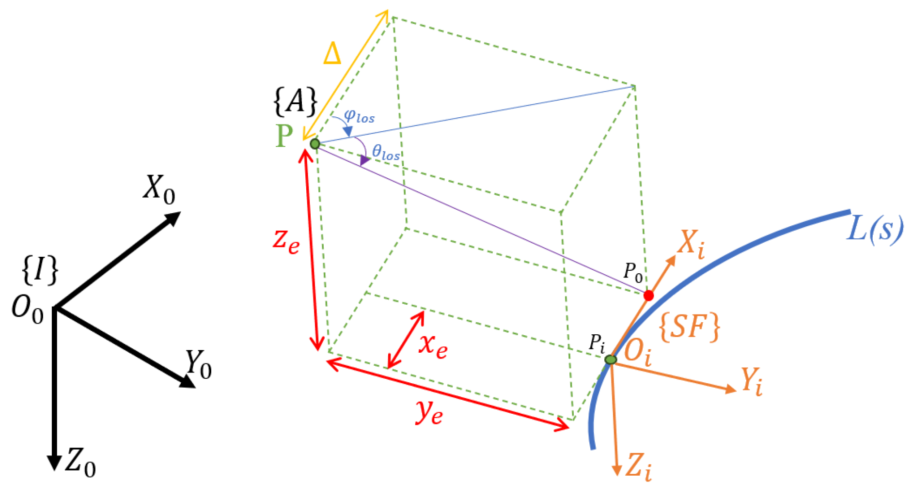
In this study, a look-ahead distance-based LOS guidance method is employed. Specifically, a tracking target point is defined at a distance $\Delta$ ahead of point P, which is the projection of the robot’s current position onto the desired path L, along the tangent direction at that point. The desired yaw and pitch angles are computed with respect to the target point and are then transformed into the corresponding attitude angles in the earth-fixed coordinate frame via coordinate transformation. Finally, a controller is designed to drive the robot’s actual attitude angles to converge to the desired values.

Figure 4 illustrates the reference coordinate frames used in the 3D LOS guidance strategy. SF denotes the tangential coordinate frame at point $P_i$ on the desired path L(s), representing the virtual tracking point. The angles ${\theta }_i$ and ${\phi }_i$ correspond to the pitch and yaw angles between the tangential frame at $P_i$ and the earth-fixed frame I, and can be computed directly from the geometry of the desired path L(s). The parameter $\Delta$ represents a user-defined look-ahead distance.

To facilitate the computation of the desired yaw and pitch angles, the tracking error is transformed from the inertial coordinate frame I to the tangential coordinate frame SF:

$$\left[\begin{array}{c}{x}_e\\ y_e\\ z_e\end{array}\right]=\left[\begin{array}{ccc}\cos {\theta }_i\cos {\phi }_i& \cos {\theta }_i\sin {\phi }_i& -\sin {\theta }_i\\ -\sin {\phi }_i& \cos {\phi }_i& 0\\ \sin {\theta }_i\cos {\phi }_i& \sin {\theta }_i\sin {\phi }_i& \cos {\theta }_i\end{array}\right]\left[\begin{array}{c}x-x_i\\ y-y_i\\ z-z_i\end{array}\right]$$

(17)

where $(x,y,z)$ represents the actual position P of the robot in the inertial coordinate frame I, while $(x_i,y_i,z_i)$ denotes the position of point $P_i$ on the desired path, also expressed in frame I. By differentiating the above expression, the error dynamics can be derived as follows [21]:

$$\left\{\begin{array}{c}{x}_e^{\prime }=U\cos {\phi }_{los}\cos {\theta }_{los}+{\phi }_i^{\prime }\cos {\theta }_i{y}_e-{\theta }_i^{\prime }{z}_e-U_i^{*}{s}^{\prime }\\ y_e^{\prime }=U\sin {\phi }_{los}\cos {\theta }_{los}-{\phi }_i^{\prime }\cos {\theta }_i{x}_e-{\phi }_i^{\prime }\sin {\theta }_i{z}_e\\ z_e^{\prime }=-U\sin {\theta }_{los}+{\theta }_i^{\prime }{x}_e+{\phi }_i^{\prime }\sin {\theta }_i{y}_e\\ U_i^{*}=\sqrt{{x_i^{\prime }}^2+{y_i^{\prime }}^2+{z_i^{\prime }}^2}\end{array}\right.$$

(18)

Since the snorkeling motion is controlled using a PID controller, a precise dynamic model is not required. Therefore, only the kinematic constraint associated with the lateral tracking error $y_e$ is considered in the control design. To ensure that the trajectory generated by the LOS guidance remains close to the desired path, the convergence and stability of the guidance system are analyzed in the vicinity of the equilibrium point $y_e=0$. Assuming that the robot accurately follows the desired path during tracking, the corresponding desired yaw angle ${\phi }_{de}$ and pitch angle ${\theta }_{de}$ are given by:

$$\left\{\begin{array}{c}{\phi }_{de}={\phi }_i-{\phi }_{los}\\ {\theta }_{de}={\theta }_i-{\theta }_{los}\\ {\phi }_{los}=\arctan ({\displaystyle \frac{y_e}{\Delta }})\\ {\theta }_{los}=\arctan ({\displaystyle \frac{z_e}{\sqrt{y_e^2+{\Delta }^2}}})\end{array}\right.$$

(19)

To facilitate subsequent controller design, the error dynamics equation is appropriately simplified. When the robot’s actual path remains close to the desired path, it is assumed that ${\phi }_{los}\to 0$, ${\theta }_{los}\to 0$, and the actual yaw angle $\phi \to {\phi }_{de}$; therefore, $\sin ({\phi }_i-{\phi }_{de})\to {\phi }_i-{\phi }_{de}\to {\phi }_i-\phi$ and $\cos ({\theta }_i-\theta )\to 1$. By simplifying Equation (18), the following expression is obtained:

$$y_e^{\prime }=U({\phi }_i-\phi )-{\phi }_i^{\prime }(\cos {\theta }_i{x}_e+\sin {\theta }_i{z}_e)$$

(20)

The variables ${\phi }_i^{\prime }$ and ${\theta }_i$ in the equation are associated with the virtual tracking point $P_i$. Since this study focuses on designing a path tracking algorithm for bionic-driven amphibious robots operating under nonlinear and time-varying force conditions, the desired path is simplified to facilitate algorithm implementation. Specifically, the path adopted in this work is composed of multiple piecewise linear segments, with curvature discontinuities occurring only at the turning points. Within each segment, the curvature remains constant, and its rate of change is zero. Therefore, in the computation of Equation (20), terms related to curvature variation can be neglected.

5.2. NMPC-Based Horizontal Motion Controller

In this study, the horizontal motion tracking controller is designed not only to accurately follow the desired trajectory in the horizontal plane, but also to maintain the robot’s attitude balance and stability during motion. Considering the strong nonlinear characteristics of underwater robot dynamics and the presence of practical constraints such as actuator saturation, a comprehensive analysis is conducted on the applicability and limitations of conventional control methods, including PID control, fuzzy control, and sliding mode control. Based on the results of this analysis, the NMPC strategy is adopted due to its capability for multi-objective optimization, its suitability for nonlinear dynamic systems, and its ability to explicitly handle system constraints.

MPC is a model-based control method that operates on the principle of rolling optimization. At each sampling instant, it predicts the system’s future behavior, solves a constrained optimal control problem over a finite prediction horizon, and applies only the first control input to the system. This process is repeated at every time step, enabling continuous dynamic optimization [22]. NMPC extends MPC to nonlinear dynamic systems. In each sampling period, it solves an optimal control problem that incorporates a nonlinear system model along with input, state, and output constraints. This typically results in a nonlinear programming (NLP) problem, which requires advanced numerical optimization techniques for real-time implementation [23]. Compared to linear MPC, NMPC entails higher computational complexity and longer solution times, but offers superior control performance for systems with significant nonlinearities.

In the preceding sections, the robot’s dynamic model and the LOS guidance strategy were analyzed, and the corresponding state equations governing motion and path tracking were derived. Based on the two control objectives, the state vector is defined as $x=[y_e,\overline{\phi },u,v,w,p,q,r]$. For notational simplicity, let $\overline{\phi }={\phi }_i-\phi$, and define the control input vector as $\mathit{u}=[{\phi }_{3al},{\phi }_{3ar}]$, representing the flapping amplitudes of the left and right foot-wings, respectively. The state-space equation can then be expressed as:

$$\left\{\begin{array}{c}{\mathit{x}}^{\prime }=\mathit{f}(\mathit{x},\mathit{u})\\ \mathit{y}=\mathit{C}\mathit{x}\end{array}\right.$$

(21)

$$\left[\begin{array}{c}{y^{\prime }}_e\\ {\overline{\phi }}^{\prime }\\ u^{\prime }\\ v^{\prime }\\ w^{\prime }\\ p^{\prime }\\ q^{\prime }\\ r^{\prime }\end{array}\right]=\left[\begin{array}{c}U\overline{\phi }\\ r\\ 0.7953wq+3.2041vr-8.9082u\left|u\right|\\ -0.2389wp-0.3121ur-1.8229v\left|v\right|\\ 4.1867vp-1.3067uq+102.48\left|w\right|\\ -0.0404uw+20.1926vw-0.0003pr-0.769qr-0.0057p\left|p\right|\\ -16.032uw+0.0909vw+0.5616pr-0.002qr-0.0034q\left|q\right|\\ -9.0188uv+0.2995pq+0.0017p^2-0.0017q^2-0.0029r\left|r\right|\end{array}\right]+\left[\begin{array}{c}0\\ 0\\ 1.0204F_{Hx}({\phi }_{3al},{\phi }_{3ar})\\ 0.3185F_{Hy}({\phi }_{3al},{\phi }_{3ar})\\ -1.333F_{Hz}({\phi }_{3al},{\phi }_{3ar})\\ 56.8182M_{Hx}({\phi }_{3al},{\phi }_{3ar})\\ 0.0234M_{Hx}({\phi }_{3al},{\phi }_{3ar})\\ 4.175M_{Hz}({\phi }_{3al},{\phi }_{3ar})\end{array}\right]$$

(22)

Both MPC and NMPC perform optimization based on a discrete-time system model. However, the dynamic model established in this study is formulated in continuous time and must therefore be discretized prior to implementation. Common discretization methods in the literature include the forward Euler method, zero-order hold (ZOH), and the fourth-order Runge–Kutta method [24]. Among these, the forward Euler method is preferred due to its simplicity and computational efficiency, and it is generally sufficient to meet typical control accuracy requirements. Accordingly, this study adopts the forward Euler method to discretize the continuous-time system equations.

$$\left\{\begin{array}{c}\mathit{x}(k+1)=\mathit{x}(k)+T_{s}f(\mathit{x}(k),\mathit{u}(k))\\ \mathit{y}(k)=C_k\mathit{x}(k)\end{array}\right.$$

(23)

where $T_s$ denotes the sampling time, which defines the discrete-time step of the controller. In this study, it is set to 0.001 s.

In constructing the objective function, multiple factors are considered, including the lateral tracking error in a horizontal motion, the deviation from the desired attitude angles, the magnitude of the control inputs, and the rate of change of these inputs (i.e., control increments). This formulation enables joint optimization of tracking accuracy and controls smoothness, ensuring both a precise trajectory following and a stable actuator behavior.

$$J(k)={\displaystyle \sum _{i=1}^{N_p}\left|\right|\mathit{x}(i|k)|{|}_Q^2}+{\displaystyle \sum _{i=1}^{N_c}\left|\right|\mathit{u}(i|k)|{|}_R^2}+{\displaystyle \sum _{i=1}^{N_c}\left|\right|{\mathit{u}}_i(i|k)-{\mathit{u}}_{i-1}(i-1|k)|{|}_P^2}$$

(24)

where ${\mathit{u}}_0(0|k)$ denotes the control input from the previous time step in the simulation model. J is the cost function, $N_p$ is the prediction horizon length, and $N_c$ is the control horizon length. Q, R, and P are the weighting matrices corresponding to the system state, control input, and control input increment, respectively. In this study, both $N_p$ and $N_c$ are set to 10, but only the first control input is applied to the system at each time step.

In designing the state weighting matrix Q, appropriate simplifications and selections were made based on the control objectives and the dynamic characteristics of the system. First, the forward velocity u is inherently generated by the flapping motion of the foot-wings and does not require explicit regulation; therefore, it is excluded from the weighting matrix. The vertical velocity www is controlled independently by a PID controller, and its associated state is similarly omitted. Additionally, the pitch rate q is primarily affected by asymmetry between the front and rear foot-wing motions. However, since the front and rear wings are set to flap synchronously in this study, q can also be neglected. As a result, the weighting matrix Q assigns nonzero weights only to the lateral position error, yaw-angle error, lateral velocity v, roll rate p, and yaw rate r.

Since the magnitudes of the state variables during system operation are significantly smaller than those of the control inputs, and the variations in control input increments are typically smaller than the absolute values of the control inputs, it is necessary to normalize the scales of these terms in the objective function. This normalization ensures a balanced trade-off among tracking accuracy, control effort, and control smoothness. Accordingly, scale unification is applied to the weighting terms in the objective function. The specific values of the weighting matrices Q, R, and P are provided in

Table 1. NMPC simulation parameters.

Simulation Parameters	Value
sampling time $T_s$	0.001 s
prediction horizon length $N_p$	10
control horizon length $N_c$	1
system state weighting matrices Q	$\mathrm{diag}([20,30,0,60,0,50,0,60])$
control input weighting matrices R	$\mathrm{diag}([0.06.0.06])$
control input increment weighting matrices P	400
state variable x	$[\pm 5,\pm 1.5,\pm 1,\pm 1,\pm 1,\pm 1,\pm 1,\pm 1]$
input lower bound $u_{\min }$	[0.6109; 0.6109] (rad)
input upper bound $u_{\max }$	[0.7854; 0.7854] (rad)

.

In practical control scenarios, it is essential to incorporate constraint conditions into the system to ensure the feasibility of control inputs and to maintain the state variables within acceptable bounds. Based on the physical limitations of the actuators and the safety requirements of system operation, the following constraints are defined in this study:

s.t.

$$\left\{\begin{array}{c}{u}_{\min }(k+i)\le u(k+i)\le u_{\max }(k+i)\begin{array}{cc}& \forall i=0,1,\dots ,N_C-1\end{array}\\ x_{\min }(k+i)\le x(k+i)\le x_{\max }(k+i)\begin{array}{cc}& \forall i=0,1,\dots ,N_P-1\end{array}\\ x(0|k)=x(k)\\ x(i+1|k)=x(k)+T_{s}f(x(i|k),u(i|k)),\forall i=0,1,\dots ,N_P-1\end{array}\right.$$

(25)

Based on simulation experiments of the robot during normal forward swimming and turning maneuvers, the approximate range of state variables can be preliminarily determined as $[\pm 5,\pm 1.5,\pm 1,\pm 1,\pm 1,\pm 1,\pm 1,\pm 1]$. Reference [17] employed a CFD-based approach to account for factors such as forward velocity and energy consumption, and determined the optimal flapping joint amplitudes to be ${\phi }_1$ = 0.6109 rad and ${\phi }_3$ = 0.6981 rad. Accordingly, this study sets the amplitude of Joint 1 to 0.6109 rad, and defines the allowable range of flapping amplitudes for all three joints as [0.6109, 0.7854], i.e., $u_{\min }$ = 0.6109 rad, $u_{\max }$ = 0.7854 rad.

6. Simulation Experiments

In this study, a physical simulation model of the foot-wing hybrid-driven amphibious robot was developed using a co-simulation platform based on SolidWorks 2022 and Simulink Simscape R2023b. The hydrodynamic and other external forces acting on the robot during motion were computed using theoretical formulations. For control optimization, MATLAB’s built-in nonlinear constrained optimization function fmincon was employed. The Sequential Quadratic Programming (SQP) algorithm was selected to numerically solve the NMPC problem.

The snorkeling motion controller adopts a PID with LOS strategy to track the target depth, with the PID parameters set to $K_P$ = 0.003, $K_I$ = 0, and $K_D$ = 0.006. The horizontal motion controller is implemented using a PID with NMPC framework for path tracking in the horizontal plane, with a prediction horizon of $N_p$ = 10, control horizon $N_c$ = 1, and time step T = 0.001.

The desired path defined in this study is a piecewise linear trajectory composed of a series of discrete coordinate points. At the initial moment, the robot is stationary and positioned at the starting point of the path. The robot’s single foot-wing performs a two-degree-of-freedom motion, consisting of a one-joint flapping motion and a three-joint vertical beating motion. During the time interval from t = 0 to 8 s, the swing amplitudes of the first and third joints are set to 0.6109 rad and 0.6981 rad, respectively, with a quarter-period phase difference between them. This configuration produces a figure-of-eight flapping motion at the foot-wing tip. The detailed coupling relationships between the joints are provided in Reference [17]. The flapping cycle is set to 1 s in the simulation. During the first 4 s, the robot undergoes an acceleration phase. Over time, the thrust and drag forces generated by the flapping motion gradually reach equilibrium, and the robot transitions to a steady-speed state after 4 s. At t = 8 s, the robot begins executing the path tracking control algorithm proposed in this study. Upon completion of the simulation, a comparison between the robot’s center-of-gravity trajectory and the desired path is presented in Figure 5.

In the figure, the green line on the bottom plane represents the projection of the reference path onto the XOY plane.

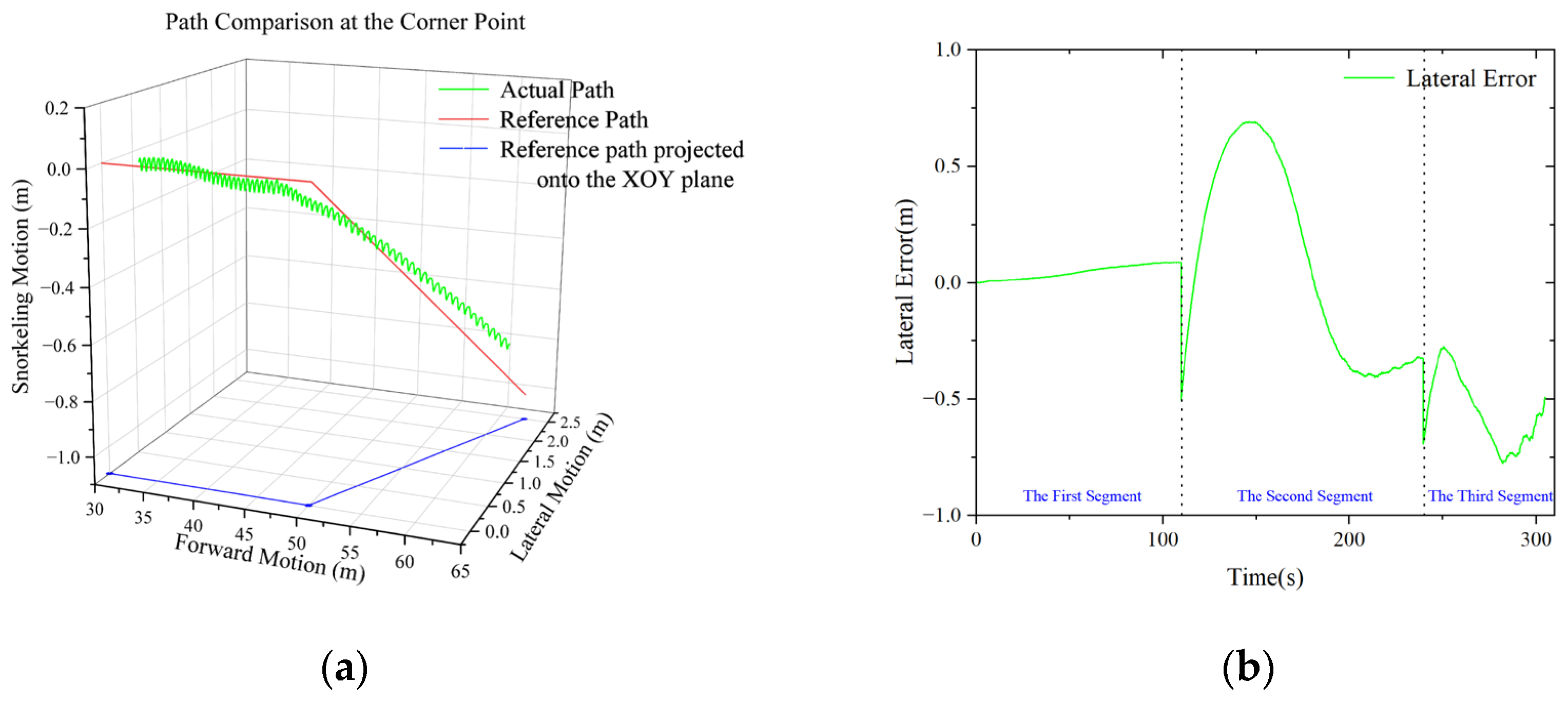
To prevent excessive path deviation at the turning points of the piecewise linear trajectory, this study introduces a preemptive waypoint-switching strategy. Specifically, when the robot’s longitudinal distance to a turning point is less than 3 m, the tracking target is switched in advance to the next waypoint. Figure 6a presents an enlarged comparison between the desired and actual trajectories at the path inflection point. This approach reserves sufficient turning space for the robot, ensuring smooth transitions and stable path tracking performance.

Figure 6b indicates that the robot can accurately follow the predefined trajectory, with the lateral tracking error remaining within a small range throughout the motion. During turning maneuvers, the proposed control algorithm effectively balances the steering torque and roll torque, enabling the robot to complete turns while maintaining stable attitude control.

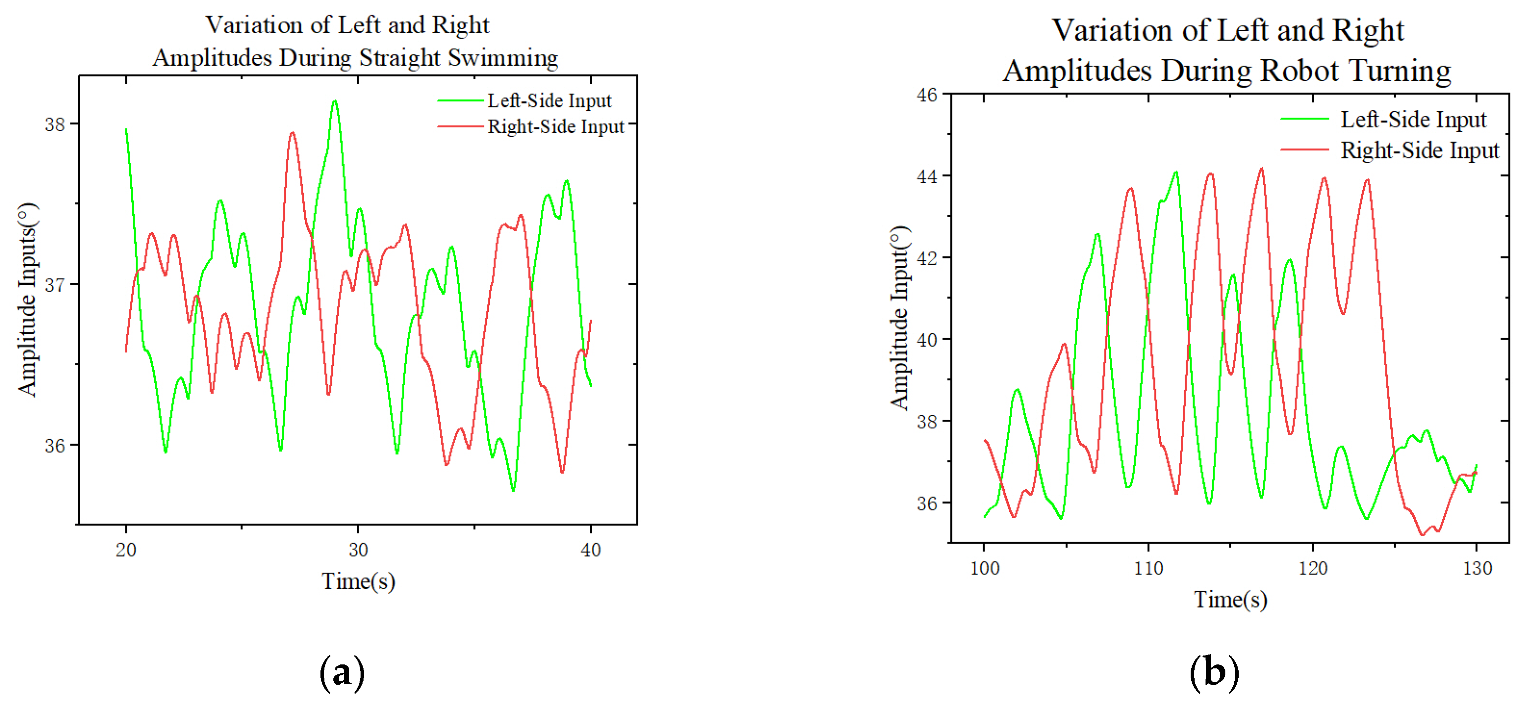
Figure 7a and Figure 7b show the amplitude inputs of the robot’s left and right foot-wings during forward locomotion and turning, respectively.

Furthermore, to verify that the proposed NMPC algorithm can achieve accurate path tracking while maintaining body attitude stability, this study selects the LOS + PID and LOS + fuzzy PID algorithms as comparative benchmarks. These methods are used to perform tracking control of the robot along the same reference path. Under the PID-based control strategy, the flapping amplitudes of the three joints on one side of the foot-wing are fixed, while those on the other side are adjusted using a PID controller to generate asymmetric flapping forces for turning control. The PID controller parameters are set to $K_P$ = 0.452, $K_I$ = 0, and $K_D$ = 1.03. In the fuzzy PID controller, the fuzzy universes of discourse for the input error e and its rate of change ec are defined as [−0.3, 0.3] and [−0.3, 0.3], respectively. The fuzzy control rules are adopted from Reference [25]. The outputs of the fuzzy inference rules are scaled by corresponding scaling factors to obtain the correction values $\Delta K_p^{\prime }$, $\Delta K_I^{\prime }$, and $\Delta K_D^{\prime }$. These correction values are then used in the following equations to compute the fuzzy PID gains $K_{fuzzy\_p}$, $K_{fuzzy\_I}$, and $K_{fuzzy\_D}$.

$$\left\{\begin{array}{c}{K}_{fuzzy\_p}=K_p^{\prime }+\Delta K_p^{\prime }\\ K_{fuzzy\_I}=K_I^{\prime }+\Delta K_I^{\prime }\\ K_{fuzzy\_D}=K_D^{\prime }+\Delta K_D^{\prime }\end{array}\right.$$

(26)

where parameters $K_p^{\prime }$, $K_I^{\prime }$, and $K_D^{\prime }$ serve as the initial values of the controller and are set the same as those used in the aforementioned PID.

Figure 8a and Figure 8b respectively present a comparison of the trajectories generated by the three algorithms during tracking of the desired path, along with the corresponding variations in the robot’s roll angular velocity p under different control methods. These results are used to comprehensively evaluate both path tracking accuracy and attitude stability.

Table 2. Comparison of path tracking experimental data.

Simulation Method	Max Error (m)	Average Error (m)	Standard Deviation (rad/s)	Simulation Time
NMPC	1.7621	0.3244	0.1262	$\approx$12 h
PID	0.7951	0.3137	0.1671	$\approx$10 min
Fuzzy PID	0.7699	0.2944	0.1337	$\approx$9 h

summarizes the simulation results of the three control methods. The evaluation metrics include maximum tracking error, average tracking error, standard deviation of roll angular velocity, and total simulation time. Here, the simulation time refers to the actual time consumed in Simulink for the model to complete the path tracking task.

As shown in the figure, all three control methods are capable of effectively tracking the desired path. Among them, the PID and fuzzy PID controllers exhibit similar maximum and average tracking errors, indicating relatively consistent and stable performance. In contrast, the NMPC method demonstrates a significantly higher maximum tracking error compared to the other two approaches, while its average error remains comparable. This suggests certain limitations in local transient response, despite maintaining acceptable overall tracking accuracy.

In terms of attitude control, the NMPC algorithm explicitly incorporates posture stability into the control process by accounting for the robot’s dynamic balance. As a result, it achieves a significantly lower standard deviation of roll angular velocity compared to the PID and fuzzy PID controllers, demonstrating superior attitude stability. The fuzzy PID controller adjusts the PID parameters in real time based on fuzzy inference rules, which helps suppress fluctuations in roll angular velocity to some extent. However, since both PID and fuzzy PID strategies are designed primarily for path tracking accuracy without considering attitude balance, roll angular velocity tends to accumulate during the later stages of the simulation. This issue becomes more pronounced during large-angle turns, where these two controllers rely mainly on yaw-angle adjustment and do not account for torque balance in other directions. As a result, lateral torque imbalance may occur, potentially leading to loss of stability or even robot overturning. In contrast, the roll angular velocity under NMPC control remains within a small range, and the robot maintains a stable posture throughout the motion. With respect to simulation time, NMPC requires solving a nonlinear optimization problem at each control step, resulting in the highest computational load and the longest simulation time. The fuzzy PID controller also performs rule matching and parameter adjustment during each cycle, which introduces additional computational overhead compared to conventional PID, thereby leading to a relatively longer simulation time.

However, several additional factors must be considered when applying the NMPC algorithm to the underwater robot investigated in this study. On one hand, the developed hydrodynamic model does not fully capture external disturbances, which reduces the controller’s robustness to unknown perturbations. On the other hand, the high computational complexity of NMPC presents challenges for real-time implementation on embedded systems. Although a relatively accurate dynamic model is established in this work, the inherent complexity and unpredictability of real underwater environments may still impact the accuracy and robustness of the controller.

A comprehensive analysis indicates that although the instantaneous tracking accuracy of NMPC may be inferior to that of conventional PID control, its overall control performance is superior in long-distance path tracking tasks. Nevertheless, in practical engineering applications, a trade-off must be made between the algorithm’s computational complexity and its real-time control capability. This trade-off remains a key challenge limiting the widespread adoption of NMPC.

7. Conclusions

This paper addresses the challenge of achieving high-precision 3D path tracking for bionically actuated amphibious robots operating in complex underwater environments characterized by periodic and time-varying thrust forces, through systematic modeling and control design. First, the hydrodynamic forces acting on the robot during underwater hovering, along with the thrust generated by foot-wing flapping, were thoroughly analyzed, leading to the development of a complete six-degree-of-freedom dynamic model. To simplify the periodic actuation inputs, an averaging method based on a scaling function was introduced. This enabled the derivation of an explicit functional relationship between the joint flapping amplitude and the resulting thrust force, thereby enhancing model controllability and facilitating controller design.

Finally, a horizontal path tracking controller was developed by integrating NMPC with the LOS guidance strategy. Simulation results demonstrate that the proposed control approach not only achieves high-precision trajectory tracking, but also effectively maintains attitude stability throughout underwater motion.

Nevertheless, several limitations remain in this study. Certain secondary hydrodynamic terms were simplified during the modeling process, which may affect the overall accuracy of the dynamic model. Although the averaging-based model reduces computational complexity, it still retains a relatively complex structure that may hinder the real-time performance and implementation efficiency of the controller. Moreover, the controller design does not account for common environmental disturbances such as ocean currents and waves, which limits its robustness under complex operating conditions. In addition, the stability of the NMPC controller has not been systematically analyzed from a theoretical perspective, and thus lacks rigorous theoretical justification.

Therefore, future research should focus on more comprehensive hydrodynamic modeling, enhanced robustness to environmental disturbances, and a rigorous theoretical analysis of controller stability. These improvements are expected to enhance the practicality and engineering scalability of the proposed control system.