Global Fast Terminal Sliding Mode Control of Underwater Manipulator Based on Finite-Time Extended State Observer

Abstract

This study investigates the trajectory-tracking control problem of a two-degree-of-freedom underwater manipulator operating in a complex disturbance environment. A dynamic model of the multi-link serial manipulator is first established. In this study, water resistance and additional mass forces acting on the manipulator are analyzed and calculated using differential analysis and the Morrison formula. To account for coupling between joints, the concept of equivalent gravity is introduced to precisely calculate the underwater manipulator’s buoyancy and gravity. As a result, a relatively accurate dynamic model of the underwater manipulator is established. To mitigate the influences of external disturbances and unmodeled parts on the manipulator, a finite-time extended state observer (FTESO) is designed to estimate system quantities that are difficult to measure directly. The robustness of the controller is enhanced using a feedforward compensation mechanism, and it is demonstrated that the observation error of the observer converges in finite time. Finally, a global fast terminal sliding mode controller (GFTSMC) is developed for trajectory tracking, integrated with the aforementioned observer, and designed to smooth and limit the controller’s output. The controller’s stability is proven using Lyapunov stability theory, and its effectiveness is verified through simulation-based comparison experiments.

1. Introduction

Since the beginning of the 21st century, underwater robots have played an increasingly vital role in underwater archaeology, underwater facility operation and maintenance, underwater target search, and other fields. As a core actuator for marine engineering equipment, underwater manipulators can be installed on a variety of platforms to perform complex underwater tasks, such as deep-sea resource exploration and emergency rescue. Their high-precision trajectory-tracking capability is crucial for ensuring successful task completion [1,2,3]. In complex marine environments, underwater manipulators must achieve fast and stable tracking of a predetermined trajectory while accounting for the combined effects of the water environment, unknown disturbances, and unpredictable contact loads. However, the manipulator system is a multi-input, multi-output, nonlinear, and strongly coupled dynamic system, which presents significant challenges for both the modeling and controller design of the underwater manipulator [4]. Therefore, these technical difficulties make research in this field particularly valuable, with important implications for both theoretical advancement and practical applications.

In recent years, scholars from various countries have conducted extensive research on the trajectory-tracking control of underwater manipulators. Traditional control methods (e.g., PID and model predictive control) frequently fail to satisfy the stringent requirements of deep-sea operations, particularly in terms of dynamic response and robustness. These shortcomings typically are due to strong model dependence, insufficient anti-interference ability, or slow convergence speeds [5,6,7,8,9,10]. In contrast, sliding mode control has the advantages of rapid response, insensitivity to parameter changes and disturbances, no need for online system identification, and simple physical implementation. It is widely used in the design of underwater manipulator controllers, and a variety of improved sliding mode control methods have been derived from it. Yuguang Zhong et al. proposed a dynamic modeling method with an improved adaptive fuzzy sliding mode control algorithm for multi-link underwater manipulators. The control gain is adjusted by the fuzzy logic system to reduce underwater disturbances and suppress chattering. The effectiveness of their control method was validated through simulations [11]. Minghao Liu et al. designed a sliding mode controller for flutter suppression in underwater manipulators based on time delay estimation, aimed at achieving precise control of the underwater manipulator. Simulations and experiments show that the designed controller has better trajectory-tracking accuracy and stronger anti-interference ability than both the sliding mode controller and the one solely based on time delay estimation [12]. Zaare, Saeed et al. proposed a predefined-time nonsingular terminal sliding mode control method based on an uncertainty and speed observer, and proved the global asymptotic stability of the system within a predefined time in the presence of uncertainty. The simulation was carried out on a two-link underwater manipulator, and high-precision trajectory tracking was achieved within the predefined time [13]. Aiming at the field of fine underwater structure repair, Juzheng Mao et al. developed a new lightweight manipulator and established a trajectory-tracking control algorithm based on a disturbance observer and sliding mode control. Experiments showed that the control algorithm significantly improved the trajectory-tracking accuracy of the manipulator under high flow rate conditions [14]. Dahui Ge et al. studied the trajectory-tracking control problem of a two-joint underwater manipulator in a wave environment. They combined sliding mode control with different reaching laws, and carried out experiments under different wave conditions. The experiments showed that the exponential reaching law of sliding mode control performs best in trajectory tracking and chattering suppression [15]. Lihui Liao et al. proposed an adaptive super-twisting sliding mode control method based on an extended state observer, designed to achieve high-precision position control of underwater manipulators in the presence of uncertainties and external disturbances. The effectiveness of the controller was verified through simulations and comparative experiments with the adaptive fuzzy sliding mode control method [16]. Borlaug, Ida Louise G et al. introduced a sliding mode control law with an adaptive-gain super-twisting algorithm and proposed a high-order sliding mode observer for state estimation in the control of an underwater swimming manipulator. Experiments showed that the proposed method significantly reduced position error and enhanced immunity compared to the linear PD controller [17]. Yang Wang et al. designed a finite-time sliding mode control method based on a fixed-time observer to address the control problem of flexible joint manipulators. The effectiveness of the proposed scheme was validated through numerical simulations, showing that it simplifies the measurement system while ensuring control accuracy [18]. Yazhou Fan et al. designed a novel controller based on an adaptive arctangent nonsingular terminal sliding mode control method to handle uncertainties and disturbances in complex underwater environments. Compared with the traditional nonsingular terminal sliding mode controller and the non-adaptive arctangent nonsingular variant, the proposed controller achieved accelerated convergence and improved tracking precision [19]. Haobin Xue et al. analyzed hydrodynamic effects on a flexible connecting rod manipulator and designed a piecewise smoother to reduce the coupling vibration between water flow and the rod. Simulation results verified the effectiveness of the control method, showing a significant reduction in the vibration amplitude of the connecting rod compared to traditional methods [20]. Wen Fu et al. proposed an adaptive sliding mode control method for underwater manipulators based on nonlinear dynamic model compensation, aimed at achieving precise control in complex underwater environments. Comparative results demonstrated the proposed method’s superiority in both tracking accuracy and system stability over the adaptive sliding mode control incorporating dual-loop PID and RBF neural network [21]. Kangsen Huang et al. formulated a robust fuzzy logic sliding mode control method to improve the control accuracy and anti-interference capability of a two-joint underwater manipulator. Compared with the traditional sliding mode control, the proposed method achieved smaller tracking errors and faster convergence speeds [22]. Zengcheng Zhou et al. developed an adaptive nonsingular fast terminal sliding mode control method for underwater manipulators subject to unknown time-varying external disturbances, which achieved precise trajectory tracking [23]. Fei Wang et al. formulated a fuzzy sliding mode tracking control method based on RBFNN for a three-joint underwater manipulator, with its efficacy validated through numerical simulations [24]. To address the problem of actuator saturation in the process of underwater vehicle trajectory tracking, Zhu Danjie et al. applied fuzzy logic methodology to dynamically constrain the amplitude of output signals, ensuring that all control signals remain strictly within the actuator’s effective operational range. They also proposed a fuzzy backstepping−sliding mode composite control method. Simulation results indicated that the method is suitable for precise operational tasks in complex marine environments [25]. Phuong Nam Dao et al. proposed two novel TSMC schemes to overcome the limitations of conventional TSMC in handling time-varying communication delays and actuator saturation. The controller’s tracking performance under the influence of actuator saturation and variable time communication delay was validated through simulation experiments [26]. Zhenhua Zhao et al. proposed a double-edge continuous terminal sliding mode control method based on an enhanced nonlinear disturbance observer to handle high-order time-varying disturbances in teleoperation systems. The designed bilateral controller not only guarantees the continuity of the control action, but also converges the position and forces tracking errors to a small bounded region, despite these high-order time-varying disturbances. The effectiveness of the proposed method was verified through simulations [27].

In summary, while extensive research has been conducted on underwater manipulator trajectory-tracking control, significant challenges remain. These include the precise modeling of underwater manipulators, hydrodynamic compensation, and underwater disturbance rejection. To enhance the trajectory-tracking performance of underwater manipulators, this study proposes a global fast terminal sliding mode control (GFTSMC) method based on a finite-time extended state observer. The main contributions are as follows:

1. A dynamic model of the manipulator was derived using the Lagrange equation. The Morrison equation was employed to calculate water resistance and additional mass forces. Joint coupling effects in the marine environment, as well as buoyancy and water resistance, were considered, resulting in a more accurate dynamic model of the underwater manipulator;

2. A finite-time extended state observer (FTESO) was designed for state estimation, with feedforward compensation applied in the controller. It is strictly proved that the proposed extended state observer converges in finite time. The FTESOs detailed in this paper were compared with the extended state observers in [28,29], demonstrating superior observability;

3. A global fast terminal sliding mode controller was developed and integrated with the above FTESO. It was applied for trajectory-tracking control of an underwater manipulator, incorporating a smooth limiting design for the control output. The asymptotic stability of the designed controller is proven using the Lyapunov method. The experimental results demonstrate that the proposed control method maintains tracking accuracy even under external underwater disturbances.

The remaining sections of this paper are arranged as follows: The second section presents the dynamic model of the underwater manipulator. The third section presents the design of the global fast terminal sliding mode controller of the underwater manipulator based on the finite-time extended state observer and proves its stability. The fourth section describes the simulation experiment and discusses the results. Finally, the fifth section provides the conclusion.

2. Problem Formation

2.1. Dynamic Model of Land Manipulator

The dynamic model of the manipulator is mainly used to describe the force and torque acting on each joint while the manipulator is in motion. Inspired by [11], the dynamic model of multi-joint serial manipulator can be described by the following formula:

$$M\left(\theta \right)\ddot{\theta }+C\left(\theta ,\dot{\theta }\right)\dot{\theta }+G\left(\theta \right)=\mathit{\tau }$$

(1)

where $\theta$, $\dot{\theta }$, $\ddot{\theta }$ represent the angle, angular velocity, and angular acceleration of the manipulator joint, respectively; $M\in {\mathit{R}}^{n\times n}$ represents the inertia matrix of the manipulator system; $C$ represents the Coriolis force and centripetal force matrix; $G\in {\mathit{R}}^n$ represents the gravity term matrix; $\mathit{\tau }$ denotes the joint torque of the manipulator [11].

2.2. Hydrodynamic Model and Analysis

Underwater robotic manipulators are subject to dynamic coupling effects between joint movements and environmental factors during operation. Compared with manipulators operating on land, underwater manipulators are mainly affected by buoyancy, lift, water resistance, and additional mass forces. A schematic diagram of the underwater manipulator is shown in Figure 1. The force $F$ of the underwater manipulator in water can be expressed as follows:

$$F_{\mathrm{w}}=F_{\mathrm{d}}+F_{\mathrm{m}}+F_{\mathrm{f}}+F_{\mathrm{l}}$$

(2)

where $F_{\mathrm{d}}$ refers to the water resistance of the manipulator moving in water; $F_{\mathrm{m}}$ represents the additional mass force on the underwater manipulator; $F_{\mathrm{f}}$ is the buoyancy of the underwater manipulator; $F_{\mathrm{l}}$ denotes the lift force of the underwater manipulator.

Before proceeding with the hydrodynamic modeling and analysis of the manipulator, the following reasonable assumptions were made:

• This study focuses solely on the self-motion of the manipulator under water, specifically its hydrodynamic modeling in a hydrostatic environment;
• The underwater manipulator is modeled as a regular cylinder with a uniform mass distribution. It has no airfoil structure and is unaffected by lift, that is, $F_{\mathrm{l}}=\mathbf{0}$;
• The center of mass of the underwater manipulator and its center of buoyancy can be aligned, and the weight of the manipulator is assumed to exceed the buoyant force;
• Fluid is considered incompressible;
• External disturbances acting on the underwater manipulator are bounded.

Next, the water resistance and additional mass force of the underwater manipulator are calculated using the Morrison formula. The specific form of the Morrison formula is as follows:

$$\mathrm{d}F=\mathrm{d}{F}_{\mathrm{d}}+\mathrm{d}{F}_{\mathrm{m}}={\displaystyle \frac{1}{2}}\rho c_{\mathrm{d}}Dv‖v‖\mathrm{d}l+\rho c_{\mathrm{m}}A{\displaystyle \frac{\mathrm{d}v}{\mathrm{d}t}}\mathrm{d}l$$

(3)

where $\rho$ denotes the density of water; $c_{\mathrm{d}}$ represents the water resistance coefficient; $D$ denotes the diameter of the connecting rod of the manipulator; $v$ represents the velocity function of the connecting rod; $c_{\mathrm{m}}$ represents the additional mass force coefficient; $A$ represents the projection area of the manipulator connecting rod perpendicular to the direction of water flow velocity.

2.2.1. Analysis of Water Resistance

According to Formula (3), the water resistance and water resistance torque of the manipulator connecting rod can be obtained as follows:

$${\mathbf{F}}_{\mathrm{d}}=\frac{1}{2}\rho c_{\mathrm{d}}D{\int }_0^L\mathbf{v}(x)\Vert \mathbf{v}(x)\Vert \mathrm{d}x$$

(4)

$${\mathit{\tau }}_{\mathrm{d}}=\frac{1}{2}\rho c_{\mathrm{d}}D{\int }_0^L{[x\hspace{1em}0\hspace{1em}0]}^{\top }\mathbf{v}(x)\Vert \mathbf{v}(x)\Vert \mathrm{d}x$$

(5)

where $v(x)$ denotes the normal velocity of the connecting rod; $L$ denotes the length of the connecting rod; $\mathrm{d}x$ denotes the unit thickness of the connecting rod. When the force of joint 1 rotates, it drives the displacement of both connecting rod 1 and connecting rod 2. $v_{1-1}$ and $v_{2-2}$ represent the normal velocities generated by the angular velocities of joint 1 and joint 2, respectively, on the unit length of connecting rod 1. $v_{2-1}$ represents the normal velocity generated by the angular velocity of joint 2 on the unit length of the connecting rod. According to the analysis and calculations of the motion diagram of the underwater manipulator, it is concluded that $v_{1-1}={\dot{\theta }}_1{x}_1$, $v_{2-1}={\dot{\theta }}_1\left(L_1\cos {\theta }_2+x_2\right)$, $v_{2-2}={\dot{\theta }}_2{x}_2$. Binding Formula (5), the water resistance moment of joint 1 is obtained as the following:

$$\begin{array}{cc}\hfill {\mathit{\tau }}_{d1}& ={\displaystyle \frac{1}{2}}\rho c_{\mathrm{d}}{D}_1{\displaystyle {\int }_0^{L_1}{r}_{1-1}}{v}_{1-1}‖v_{1-1}‖\mathrm{d}{x}_1 \hfill \\ \hfill & +{\displaystyle \frac{1}{2}}\rho c_{\mathrm{d}}{D}_2{\displaystyle {\int }_0^{L_2}{r}_{2-1}}{v}_{2-1}‖v_{2-1}‖\mathrm{d}{x}_2\hfill \\ \hfill & ={\displaystyle \frac{1}{2}}\rho c_{\mathrm{d}}{D}_1{\displaystyle {\int }_0^{L_1}{\dot{\theta }}_1}{x}_1‖{\dot{\theta }}_1{x}_1‖x_1\mathrm{d}{x}_1 \hfill \\ \hfill & +{\displaystyle \frac{1}{2}}\rho c_{\mathrm{d}}{D}_2{\displaystyle {\int }_0^{L_2}\left[{\dot{\theta }}_1{L}_1\cos {\theta }_2+({\dot{\theta }}_1+{\dot{\theta }}_2)x_2\right]} \hfill \\ \hfill & \hspace{1em} \cdot (L_1\cos {\theta }_2+x_2)‖{\dot{\theta }}_1{L}_1\cos {\theta }_2+({\dot{\theta }}_1+{\dot{\theta }}_2)x_2‖\mathrm{d}{x}_2\hfill \end{array}$$

(6)

When the force of joint 2 rotates, it drives the connecting rod 2 to produce displacement. For $\mathrm{d}{x}_2$ on connecting rod 2, the angular velocity around the joint axis $Z_2$ is ${\omega }_2={\dot{\theta }}_2$, the direction vector is $r_{2-2}=x_2$, and the normal velocity is $v_{2-2}={\omega }_2{r}_{2-2}={\dot{\theta }}_2{x}_2$. From Formula (5), it can be concluded that the water resistance torque of joint 2 is

$$\begin{array}{cc}\hfill {\mathit{\tau }}_{d2}& ={\displaystyle \frac{1}{2}}\rho c_d{D}_2{\displaystyle {\int }_0^{L_2}{r}_{2-2}}{v}_{2-2}‖v_{2-2}‖\mathrm{d}{x}_2\hfill \\ \hfill & ={\displaystyle \frac{1}{2}}\rho c_d{D}_2{\displaystyle {\int }_0^{L_2}\left[{\dot{\theta }}_1{L}_1\cos {\theta }_2+({\dot{\theta }}_1+{\dot{\theta }}_2)x_2\right]}\hfill \\ \hfill & \hspace{1em} \cdot ‖{\dot{\theta }}_1{L}_1\cos {\theta }_2+({\dot{\theta }}_1+{\dot{\theta }}_2)x_2‖\cdot x_2\mathrm{d}{x}_2\hfill \end{array}$$

(7)

2.2.2. Analysis of Additional Mass Force

According to Formula (3), the additional mass force and additional mass moment of the manipulator connecting rod can be obtained as follows:

$$F_m={\displaystyle \frac{\pi }{4}}\rho D^2{c}_m{\displaystyle {\int }_0^L\frac{dv(x)}{dt}dx}$$

(8)

$${\mathit{\tau }}_m={\displaystyle \frac{\pi }{4}}\rho D^2{c}_m{\displaystyle {\int }_0^L{\left[\begin{array}{ccc}x& 0& 0\end{array}\right]}^{\top }}{\displaystyle \frac{\mathrm{d}v(x)}{\mathrm{d}t}}\mathrm{d}x$$

(9)

According to Formula (8), when the force of joint 1 rotates, the additional mass moment of the joint 1 can be obtained as follows:

$$\begin{array}{cc}\hfill {\mathit{\tau }}_{m1}& ={\displaystyle \frac{\pi }{4}}\rho {D_1}^2{c}_m{\displaystyle {\int }_0^{L_1}{r}_{1-1}}{\displaystyle \frac{d{v}_{1-1}}{dt}}\mathrm{d}{x}_1 \hfill \\ \hfill & +{\displaystyle \frac{\pi }{4}}\rho {D_2}^2{c}_m{\displaystyle {\int }_0^{L_2}{r}_{2-1}}{\displaystyle \frac{d{v}_{2-1}}{dt}}\mathrm{d}{x}_2\hfill \\ \hfill & ={\displaystyle \frac{\pi }{4}}\rho {D_1}^2{c}_m{\displaystyle {\int }_0^{L_1}{x}_1 }{\displaystyle \frac{d({\dot{\theta }}_1{x}_1)}{dt}}\mathrm{d}{x}_1 \hfill \\ \hfill & +{\displaystyle \frac{\pi }{4}}\rho {D_2}^2{c}_m{\displaystyle {\int }_0^{L_2}\left[L_1\cos {\theta }_2+x_2\right]} \hfill \\ \hfill & \hspace{1em} \cdot {\displaystyle \frac{d\left[{\dot{\theta }}_1{L}_1\cos {\theta }_2+({\dot{\theta }}_1+{\dot{\theta }}_2)x_2\right]}{dt}}\mathrm{d}{x}_2\hfill \end{array}$$

(10)

When the force of joint 2 rotates, the additional mass moment of joint 2 can be obtained in the same way:

$$\begin{array}{l}{\mathit{\tau }}_{m2}={\displaystyle \frac{\pi }{4}}\rho {D_2}^2{c}_m{\displaystyle {\int }_0^{L_2}{r}_{2-2}}{\displaystyle \frac{d{v}_{2-2}}{dt}}\mathrm{d}{x}_2\\ \begin{array}{cc}& =\end{array}{\displaystyle \frac{\pi }{4}}\rho {D_2}^2{c}_m{\displaystyle {\int }_0^{L_2}{x}_2}{\displaystyle \frac{d\left[{\dot{\theta }}_1{L}_1\cos {\theta }_2+({\dot{\theta }}_1+{\dot{\theta }}_2)x_2\right]}{dt}}\mathrm{d}{x}_2\end{array}$$

(11)

By summarizing Formulas (6), (7), (10) and (11), the water resistance matrix and the additional mass force matrix of the two-link manipulator can be obtained as follows:

$${\mathit{\tau }}_d={\left(\begin{array}{cc}{\mathit{\tau }}_{d1}& {\mathit{\tau }}_{d2}\end{array}\right)}^{\top }$$

(12)

$${\mathit{\tau }}_m={\left(\begin{array}{cc}{\mathit{\tau }}_{m1}& {\mathit{\tau }}_{m2}\end{array}\right)}^{\top }$$

(13)

Moreover, the two sets of matrices have the following relationship with the two joint angles:

$${\mathit{\tau }}_d=C_d\left(\theta ,\dot{\theta }\right)\dot{\theta }$$

(14)

$${\mathit{\tau }}_m=M_m\left(\theta \right)\ddot{\theta }+C_m\left(\theta ,\dot{\theta }\right)\dot{\theta }$$

(15)

where $M_m$ is the inertia matrix; $C_d$ and $C_m$ are the Coriolis force and centripetal force matrix, respectively.

2.2.3. Analysis of Equivalent Gravity

When the manipulator is submerged in water, it will continue to be affected by buoyancy. Under the assumed conditions, the direction of buoyancy is always opposite to the direction of the gravity, and the centers of buoyancy and gravity are the same. Therefore, the concept of equivalent gravity can be introduced to express the resultant force of gravity and buoyancy of the underwater manipulator:

$$F_{G_{\mathrm{i}}}=m_{{\mathrm{l}}_{\mathrm{i}}}g-V_{{\mathrm{l}}_{\mathrm{i}}}\rho g=m_{{\mathrm{l}}_{\mathrm{i}}}\left(1-{\displaystyle \frac{\rho }{{\rho }_{\mathrm{m}}}}\right)$$

(16)

In the formula, $F_{G_{\mathrm{i}}}$ represents the equivalent gravity of the $\mathrm{i}$ th connecting rod; $m_{{\mathrm{l}}_{\mathrm{i}}}$ represents the mass of the connecting rod $\mathrm{i}$; $\rho$ represents the density of water; ${\rho }_{\mathrm{m}}$ represents the density of the manipulator connecting rod; $g$ represents the acceleration of gravity; $V_{{\mathrm{l}}_{\mathrm{i}}}$ represents the volume of the manipulator connecting rod $\mathrm{i}$.

Combined with the Formulas (12)–(16), it can be concluded that the dynamic model of the manipulator with hydrodynamic term is as follows:

$$M_{\mathrm{w}}\left(\theta \right)\ddot{\theta }+C_{\mathrm{w}}\left(\theta ,\dot{\theta }\right)\dot{\theta }+G_{\mathrm{w}}\left(\theta \right)={\mathit{\tau }}_{\mathrm{w}}$$

(17)

in which $M_{\mathrm{w}}\left(\theta \right)=M\left(\theta \right)+M_{\mathrm{m}}\left(\theta \right)$, $C_{\mathrm{w}}\left(\theta ,\dot{\theta }\right)=C\left(\theta ,\dot{\theta }\right)+C_{\mathrm{m}}\left(\theta ,\dot{\theta }\right)+C_{\mathrm{d}}\left(\theta ,\dot{\theta }\right)$, $G_{\mathrm{w}}\left(\theta \right)=G_{\mathrm{f}}\left(\theta \right)$, ${\mathit{\tau }}_{\mathrm{w}}=\mathit{\tau }+{\mathit{\tau }}_{\mathrm{d}}+{\mathit{\tau }}_{\mathrm{m}}$. After considering the unknown disturbance ${\mathbf{d}}_{\mathrm{w}}$, the dynamic equation of the underwater manipulator in Formula (17) can be rewritten as

$$M_{\mathrm{w}}\left(\theta \right)\ddot{\theta }+C_{\mathrm{w}}\left(\theta ,\dot{\theta }\right)\dot{\theta }+G_{\mathrm{w}}\left(\theta \right)={\mathit{\tau }}_{\mathrm{w}}+d_{\mathrm{w}}$$

(18)

Since the disturbance of the manipulator in practical engineering is not greater than its limit, the unknown disturbance could be considered bounded. The state equation of the system is derived from Formula (18):

$$\left\{\begin{array}{l}{x}_1=\theta \\ {\dot{x}}_1=x_2\\ {\dot{x}}_2={M_{\mathrm{w}}}^{-1}(\theta )({\mathit{\tau }}_{\mathrm{w}}+{\mathbf{d}}_{\mathrm{w}}-C_{\mathrm{w}}\left(\theta ,\dot{\theta }\right)-G_{\mathrm{w}}\left(\theta \right))\\ y=x_1\end{array}\right.$$

(19)

where $x_1={\left(\begin{array}{cc}{\theta }_1& {\theta }_2\end{array}\right)}^{\top }$ and $x_2={\left(\begin{array}{cc}{\dot{\theta }}_1& {\dot{\theta }}_2\end{array}\right)}^{\top }$ denote the state variables of the system.

3. Design of FTESO−GFTSMC

In this section, to achieve high-precision trajectory-tracking control of an underwater manipulator in an environment with unknown disturbances, a global fast terminal sliding mode control strategy based on a finite-time extended state observer is proposed. The controller incorporates feedforward compensation, enabled by the FTESO’s finite-time accurate observation of unmeasurable system states and lumped disturbances. In order to improve trajectory-tracking accuracy and reduce chattering in sliding mode control, a global fast terminal sliding mode controller was developed, with limited controller output to protect the actuator.

3.1. Design of Finite-Time Extended State Observer

A schematic diagram of the finite-time extended state observer is shown in Figure 2.

According to Formula (19), the extended state can be defined as

$$x_3={M_{\mathrm{w}}}^{-1}(\theta )({\mathbf{d}}_{\mathrm{w}}-C_{\mathrm{w}}\left(\theta ,\dot{\theta }\right)-G_{\mathrm{w}}\left(\theta \right))$$

(20)

According to the state equation, the extended state observer of this system is established as the following:

$$\left\{\begin{array}{l}{\tilde{x}}_1={\widehat{x}}_1-x_1\\ {\dot{\widehat{x}}}_1={\widehat{x}}_2-k_{1}si{g}^{{\alpha }_1}({\tilde{x}}_1)-{\eta }_1\mathrm{sgn}({\tilde{x}}_1)\\ {\dot{\widehat{x}}}_2={\widehat{x}}_3+{M_{\mathrm{w}}}^{-1}(\theta ){\mathit{\tau }}_{\mathrm{w}}-k_{2}si{g}^{{\alpha }_2}({\tilde{x}}_1)-{\eta }_2\mathrm{sgn}({\tilde{x}}_1)\\ {\dot{\widehat{x}}}_3=-k_{3}si{g}^{{\alpha }_3}\left({\tilde{x}}_1\right)-{\eta }_3\mathrm{sgn}({\tilde{x}}_1)\end{array}\right.$$

(21)

where ${\widehat{x}}_1$ represents the estimated value of the joint angle; ${\widehat{x}}_2$ represents the estimated value of the joint angular velocity; ${\widehat{x}}_3$ represents the estimated value of the extended state; ${\tilde{x}}_1={\widehat{x}}_1-x_1$ represents the error of the designed observer; $k_{\mathrm{i}}$ and ${\eta }_{\mathrm{i}}$ represent the positive parameters of the designed observer $\left(\mathrm{i}=1,2,3\right)$; ${\displaystyle \frac{2}{3}}<{\alpha }_1<1$, ${\alpha }_2=2{\alpha }_1-1$, ${\alpha }_2=2{\alpha }_1-1$, ${\alpha }_3=3{\alpha }_1-2$, $si{g}^{{\alpha }_i}({\tilde{x}}_1)={\left|{\tilde{x}}_1\right|}^{{\alpha }_i}\mathrm{sgn}\left({\tilde{x}}_1\right)\left(i=1,2,3\right)$, $\mathrm{sgn}\left(·\right)$ is the sign function.

According to Formulas (19) and (22), the observer error equation is obtained as follows:

$$\left\{\begin{array}{l}{\dot{\tilde{x}}}_1={\tilde{x}}_2-k_{1}si{g}^{{\alpha }_1}({\tilde{x}}_1)-{\eta }_1\mathrm{sgn}({\tilde{x}}_1)\\ {\dot{\tilde{x}}}_2={\tilde{x}}_3-k_{2}si{g}^{{\alpha }_2}({\tilde{x}}_1)-{\eta }_2\mathrm{sgn}({\tilde{x}}_1)\\ {\dot{\tilde{x}}}_3=-{\dot{x}}_3-k_{3}si{g}^{{\alpha }_3}\left({\tilde{x}}_1\right)-{\eta }_3\mathrm{sgn}({\tilde{x}}_1)\end{array}\right.$$

(22)

Theorem 1.

For the underwater manipulator model described in (19), in the presence of unknown dynamics and external disturbances—and satisfying assumptions 1–5—the FTESO established in (22) can be used to estimate external disturbances, with the estimation error converging to zero in finite time.

Proof of Theorem 1.

By simultaneously omitting $-{\eta }_1\mathrm{sgn}({\tilde{x}}_1)$, $-{\eta }_2\mathrm{sgn}({\tilde{x}}_1)$ and $-{\eta }_3\mathrm{sgn}({\tilde{x}}_1)$, the observation error of FTESO can be written as follows:

$$\left\{\begin{array}{l}{\dot{\tilde{x}}}_1={\tilde{x}}_2-k_{1}si{g}^{{\alpha }_1}({\tilde{x}}_1)\\ {\dot{\tilde{x}}}_2={\tilde{x}}_3-k_{2}si{g}^{{\alpha }_2}({\tilde{x}}_1)\\ {\dot{\tilde{x}}}_3=-{\dot{x}}_3-k_{3}si{g}^{{\alpha }_3}\left({\tilde{x}}_1\right)\end{array}\right.$$

(23)

According to Definition A1 in Appendix A, the observation error formula is ${\alpha }_1-1$ times homogeneous under the given weight $(1,{\alpha }_1,2{\alpha }_1-1)$. Defining the system matrix $\mathbf{A}=\left[\begin{array}{ccc}-k_1{\mathit{I}}_2& {\mathit{I}}_2& \mathbf{0}\\ -k_2{\mathit{I}}_2& \mathbf{0}& {\mathit{I}}_2\\ -k_3{\mathit{I}}_2& \mathbf{0}& \mathbf{0}\end{array}\right]$, which is a Hurwitz matrix. Consequently, the Lyapunov function is constructed as follows:

$${\mathit{V}}_{\alpha }({\tilde{x}}_1,{\tilde{x}}_2,{\tilde{x}}_3)={\mathit{Z}}^{\top }\mathit{P}\mathit{Z}$$

(24)

where $\mathit{Z}={\left[{\left[si{g}^{{\displaystyle \frac{1}{\delta }}}({\tilde{x}}_1)\right]}^{\top },{\left[si{g}^{{\displaystyle \frac{1}{\delta {\alpha }_1}}}({\tilde{x}}_2)\right]}^{\top },{\left[si{\mathrm{g}}^{{\displaystyle \frac{1}{\delta {\alpha }_2}}}({\tilde{x}}_3)\right]}^{\top }\right]}^{\top }$, $\delta ={\alpha }_1{\alpha }_2{\alpha }_3$. The positive definite matrix $\mathit{P}$ is the solution of Lyapunov function ${\mathit{A}}^{\top }\mathit{P}+\mathit{P}\mathit{A}=-{\mathit{I}}_6$; ${\mathit{V}}_{\alpha }({\tilde{x}}_1,{\tilde{x}}_2,{\tilde{x}}_3)$ denotes the Lyapunov function corresponding to Formula (23). According to [30], $f_{\alpha }$ can be defined as the vector field of this system. $L_{f_{\alpha }}{\mathit{V}}_{\alpha }({\tilde{x}}_1,{\tilde{x}}_2,{\tilde{x}}_3)$ is the Lie derivative of ${\mathit{V}}_{\alpha }({\tilde{x}}_1,{\tilde{x}}_2,{\tilde{x}}_3)$ along the vector field $f_{\alpha }$. From Definition A1, it follows that ${\mathit{V}}_{\alpha }({\tilde{x}}_1,{\tilde{x}}_2,{\tilde{x}}_3)$ and $L_{f_{\alpha }}{\mathit{V}}_{\alpha }({\tilde{x}}_1,{\tilde{x}}_2,{\tilde{x}}_3)$ are ${\displaystyle \frac{2}{\delta }}$ and ${\displaystyle \frac{2}{\delta }}+{\alpha }_1-1$ homogeneous of $(1,{\alpha }_1,2{\alpha }_1-1)$, respectively. According to Lemma 7.2 in [31], the following inequality holds: $L_{f_{\alpha }}{\mathit{V}}_{\alpha }({\tilde{x}}_1,{\tilde{x}}_2,{\tilde{x}}_3)\le -c_1{[{\mathit{V}}_{\alpha }({\tilde{x}}_1,{\tilde{x}}_2,{\tilde{x}}_3)]}^{\epsilon }$, where $c_1=-{\max }_{\{x_i:{\mathit{V}}_{\alpha }(x)=1\}}{L}_{f_{\alpha }}{\mathit{V}}_{\alpha }(x)$ and $\epsilon =1+{\displaystyle \frac{{\alpha }_1\delta }{2}}-{\displaystyle \frac{\delta }{2}}<1$. The Lyapunov function for the FTESO error term is selected as follows:

$${\mathit{V}}_{of}({\tilde{x}}_1,{\tilde{x}}_2,{\tilde{x}}_3)={\mathit{Z}}^{\top }\mathit{P}\mathit{Z}$$

(25)

and the definition of $\mathit{Z}$ remains consistent with the aforementioned formulation. Derivation of function ${\mathit{V}}_{of}({\tilde{x}}_1,{\tilde{x}}_2,{\tilde{x}}_3)$ leads to

$${\dot{\mathit{V}}}_{of}=L_{f_{\alpha }}{\mathit{V}}_{\alpha }({\tilde{x}}_1,{\tilde{x}}_2,{\tilde{x}}_3)+2{\mathit{Z}}^T\mathit{P}\left[\begin{array}{c}{\displaystyle \frac{-diag\left(|{\tilde{x}}_1{|}^{\frac{1}{\partial }-1}\right){\eta }_1\mathrm{sgn}({\tilde{x}}_1)}{\delta }}\\ \\ {\displaystyle \frac{-diag\left(|{\tilde{x}}_2{|}^{\frac{1}{\partial {\alpha }_1}-1}\right){\eta }_2\mathrm{sgn}({\tilde{x}}_1)}{\delta {\alpha }_1}}\\ \\ {\displaystyle \frac{-diag\left(|{\tilde{x}}_3{|}^{\frac{1}{\partial {\alpha }_2}-1}\right)({\dot{x}}_3+{\eta }_3\mathrm{sgn}({\tilde{x}}_1))}{\delta {\alpha }_2}}\end{array}\right]$$

(26)

$$\begin{array}{ll}\le -c_1{\mathit{V}}_{of}^{\epsilon }& +{\displaystyle \frac{2{\eta }_1{\lambda }_{\max }(\mathit{P})‖\mathit{Z}‖{\displaystyle \sum _{i=1}^2{\left|{\tilde{x}}_{1i}\right|}^{\frac{1}{\partial }-1}}}{\sigma }}\hfill \\ & +{\displaystyle \frac{2{\eta }_2{\lambda }_{\max }(\mathit{P})‖\mathit{Z}‖{\displaystyle \sum _{i=1}^2{\left|{\tilde{x}}_{2i}\right|}^{\frac{1}{\partial {\alpha }_1}-1}}}{\sigma {\alpha }_1}}\hfill \\ & +{\displaystyle \frac{2({\sigma }_m+{\eta }_3){\lambda }_{\max }(\mathit{P})‖\mathit{Z}‖{\displaystyle \sum _{i=1}^2{\left|{\tilde{x}}_{3i}\right|}^{\frac{1}{\partial {\alpha }_2}-1}}}{\delta {\alpha }_2}}\hfill \end{array}$$

Based on Lemma A1 in Appendix B and inequality ${(a+b)}^2\le 2(a^2+b^2)$, it can be concluded that

$${\displaystyle \sum _{i=1}^2{\left|{\tilde{x}}_{1i}\right|}^{\frac{1}{\delta }-1}}\le 2^{\delta }{\left({\displaystyle \sum _{i=1}^2{\left|{\tilde{x}}_{1i}\right|}^{\frac{1}{\delta }}}\right)}^{1-\delta }\le 2^{{\displaystyle \frac{1+\delta }{2}}}{‖\mathit{Z}‖}^{1-\delta }$$

(27)

$${\displaystyle \sum _{i=1}^2{\left|{\tilde{x}}_{2i}\right|}^{\frac{1}{\delta {\alpha }_1}-1}}\le 2^{\delta {\alpha }_1}{\left({\displaystyle \sum _{i=1}^2{\left|{\tilde{x}}_{2i}\right|}^{\frac{1}{\delta {\alpha }_1}}}\right)}^{1-\delta {\alpha }_1}\le 2^{{\displaystyle \frac{1+\delta {\alpha }_1}{2}}}{‖\mathit{Z}‖}^{1-\delta {\alpha }_1}$$

(28)

$${\displaystyle \sum _{i=1}^2{\left|{\tilde{x}}_{3i}\right|}^{\frac{1}{\delta {\alpha }_2}-1}}\le 2^{\delta {\alpha }_2}{\left({\displaystyle \sum _{i=1}^2{\left|{\tilde{x}}_{3i}\right|}^{\frac{1}{\delta {\alpha }_2}}}\right)}^{1-\delta {\alpha }_2}\le 2^{{\displaystyle \frac{1+\delta {\alpha }_2}{2}}}{‖\mathit{Z}‖}^{1-\delta {\alpha }_2}$$

(29)

Substituting the preceding inequalities into Formula (26) yields the following:

$$\begin{array}{c}{\dot{\mathit{V}}}_{of}\le -c_1{\mathit{V}}_{of}^{\epsilon }+{\displaystyle \frac{2\times 2^{\frac{1+\delta }{2}}{\eta }_1{\lambda }_{\max }(\mathit{P}){‖\mathit{Z}‖}^{2-\delta }}{\delta }}\\ +{\displaystyle \frac{2\times 2^{\frac{1+\delta {\alpha }_1}{2}}{\eta }_2{\lambda }_{\max }(\mathit{P}){‖\mathit{Z}‖}^{2-\delta {\alpha }_1}}{\delta {\alpha }_1}}\\ +{\displaystyle \frac{2\times 2^{\frac{1+\delta {\alpha }_2}{2}}({\sigma }_m+{\eta }_3){\lambda }_{\max }(\mathit{P}){‖\mathit{Z}‖}^{2-\delta {\alpha }_2}}{\delta {\alpha }_2}}\\ \le -c_1{\mathit{V}}_{of}^{\epsilon }+c_2{\mathit{V}}_{of}^{1-{\displaystyle \frac{\delta }{2}}}+c_3{\mathit{V}}_{of}^{1-{\displaystyle \frac{\delta {\alpha }_1}{2}}}+c_4{\mathit{V}}_{of}^{1-{\displaystyle \frac{\delta {\alpha }_2}{2}}}\end{array}$$

(30)

where $c_2={\displaystyle \frac{2\times 2^{\frac{1+\delta }{2}}{\eta }_1{\lambda }_{\max }(\mathit{P})}{\delta {[{\lambda }_{\min }(\mathit{P})]}^{1-\frac{\delta }{2}}}}$, $c_3={\displaystyle \frac{2\times 2^{\frac{1+\delta {\alpha }_1}{2}}{\eta }_2{\lambda }_{\max }(\mathit{P})}{\delta {\alpha }_1{\left[{\lambda }_{\min }(\mathit{P})\right]}^{1-\frac{\delta {\alpha }_1}{2}}}}$, $c_4={\displaystyle \frac{2\times 2^{\frac{1+\delta {\alpha }_2}{2}}({\sigma }_m+{\eta }_3){\lambda }_{\max }(\mathit{P})}{\delta {\alpha }_2{[{\lambda }_{\min }(\mathit{P})]}^{1-\frac{\delta {\alpha }_2}{2}}}}$.

Under the condition that $0<1-{\displaystyle \frac{\delta }{2}}<1-{\displaystyle \frac{\delta {\alpha }_1}{2}}<1-{\displaystyle \frac{\delta {\alpha }_2}{2}}<\epsilon <1$ is satisfied, the following two cases can be simplified.

When ${\mathit{V}}_{of}\ge 1$, (30) can be simplified as follows:

$${\dot{\mathit{V}}}_{of}\le -c_1{\mathit{V}}_{of}^{\epsilon }+c_o{\mathit{V}}_{of}$$

(31)

where $c_0=c_2+c_3+c_4$. Applying Lemma A2 in Appendix B, we can deduce the time when ${\mathit{V}}_{of}$ converges to ${\mathit{V}}_{of}=1$ and is bounded by $t_{o1}$, and $t_{o1}\le \ln {\displaystyle \frac{1-\frac{c_o}{c_1}{\mathit{V}}_{of}^{1-\epsilon }(0)}{c_o\epsilon -c_o}}$.

When ${\mathit{V}}_{of}<1$, Formula (30) can be expressed in a simplified form as follows:

$$\begin{array}{ll}{\dot{\mathit{V}}}_{of}& \le -c_1{\mathit{V}}_{of}^{\epsilon }+c_o{\mathit{V}}_{of}^{1-{\displaystyle \frac{\delta }{2}}}\\ & \le -c_1{\overline{c}}_o{\mathit{V}}_{of}^{\epsilon }-\left[c_1\left(1-{\overline{c}}_o\right){\mathit{V}}_{of}^{\epsilon -1+\delta /2}-c_o\right]{\mathit{V}}_{of}^{1-{\displaystyle \frac{\delta }{2}}}\end{array}$$

(32)

where $0<{\overline{c}}_0<1-{\displaystyle \frac{c_0}{c_1}}$, when ${\mathit{V}}_{of}^{\epsilon -1+\delta /2}>{\displaystyle \frac{c_o}{c_1(1-{\overline{c}}_o)}}$, ${\dot{\mathit{V}}}_{of}\le -c_1{\overline{c}}_o{\mathit{V}}_{of}^{\epsilon }$ and ${\mathit{V}}_{of}$ are reduced. According to Lemma A3 in Appendix B, the convergence time $t_{o2}\le {\displaystyle \frac{{\mathit{V}}_{of}^{1-\epsilon }(\mathit{Z}(t_{o1}))}{c_1{\overline{c}}_{o1}(1-\epsilon )}}$ is such that ${\mathit{V}}_{of}$ converges to the domain.

$${\mathit{V}}_{of}<{\left[{\displaystyle \frac{c_o}{c_1\left(1-{\overline{c}}_o\right)}}\right]}^{{\displaystyle \frac{2}{\delta {\alpha }_1}}}$$

(33)

In summary, the Lyapunov function ${\mathit{V}}_{of}$ converges to the region Formula (33) within the time $T_1=t_{o1}+t_{o2}<\infty$.

Substituting Formula (25) into Formula (33), it can be derived that

$$‖\mathit{Z}‖<{\displaystyle \frac{1}{\sqrt{{\lambda }_{\min }(\mathit{P})}}}{\left[{\displaystyle \frac{c_o}{c_1\left(1-{\overline{c}}_o\right)}}\right]}^{{\displaystyle \frac{1}{\delta {\alpha }_1}}}$$

(34)

By Lemma A1 in Appendix B, it can be concluded that

$$‖{\tilde{x}}_1‖\le {\displaystyle \sum _{i=1}^2{\left({\left|{\tilde{x}}_{1i}\right|}^{\frac{1}{\delta }}\right)}^{\delta }}\le 2^{1-\delta }{\left({\displaystyle \sum _{i=1}^2{\left|{\tilde{x}}_{1i}\right|}^{\frac{1}{\delta }}}\right)}^{\delta }\le 2^{1-\delta /2}{‖\mathit{Z}‖}^{\delta }$$

(35)

$$‖{\tilde{x}}_2‖\le {\displaystyle \sum _{i=1}^2{\left({\left|{\tilde{x}}_2\right|}^{\frac{1}{\delta {\alpha }_1}}\right)}^{\delta {\alpha }_1}}\le 2^{1-\delta {\alpha }_1}{\left({\displaystyle \sum _{i=1}^2{\left|{\tilde{x}}_{2i}\right|}^{\frac{1}{\delta {\alpha }_1}}}\right)}^{\delta {\alpha }_1}\le 2^{1-\delta {\alpha }_1/2}{‖\mathit{Z}‖}^{\delta {\alpha }_1}$$

(36)

$$‖{\tilde{x}}_3‖\le {\displaystyle \sum _{i=1}^2{\left({\left|{\tilde{x}}_{3i}\right|}^{\frac{1}{\delta {\alpha }_2}}\right)}^{\delta {\alpha }_2}}\le 2^{1-\delta {\alpha }_2}{\left({\displaystyle \sum _{i=1}^2{\left|{\tilde{x}}_{3i}\right|}^{\frac{1}{\delta {\alpha }_2}}}\right)}^{\delta {\alpha }_2}\le 2^{1-\delta {\alpha }_2/2}{‖\mathit{Z}‖}^{\delta {\alpha }_2}$$

(37)

Substituting Formula (34) into Formulas (35)–(37), respectively, leads to

$$‖{\tilde{x}}_1‖\le {\displaystyle \frac{2^{1-\delta /2}}{{\sqrt{{\lambda }_{\min }(\mathit{P})}}^{\delta }}}{\left[{\displaystyle \frac{c_o}{c_1\left(1-{\overline{c}}_o\right)}}\right]}^{{\displaystyle \frac{1}{{\alpha }_1}}}$$

(38)

$$‖{\tilde{x}}_2‖\le {\displaystyle \frac{2^{1-\delta {\alpha }_1/2}}{{\sqrt{{\lambda }_{\min }(\mathit{P})}}^{\delta {\alpha }_1}}}\left[{\displaystyle \frac{c_o}{c_1\left(1-{\overline{c}}_o\right)}}\right]$$

(39)

$$‖{\tilde{x}}_3‖\le {\displaystyle \frac{2^{1-\delta {\alpha }_2/2}}{{\sqrt{{\lambda }_{\min }(\mathit{P})}}^{\delta {\alpha }_2}}}{\left[{\displaystyle \frac{c_o}{c_1\left(1-{\overline{c}}_o\right)}}\right]}^{{\displaystyle \frac{{\alpha }_2}{{\alpha }_1}}}$$

(40)

This confirms that the observation error ${\tilde{x}}_i(i=1,2,3)$ of the proposed FTESO converges to a bounded domain in finite time. Furthermore, by appropriate selection of the parameter ${\eta }_i(i=1,2,3)$, the error ${\tilde{x}}_i(i=1,2,3)$ converges to the equilibrium state when the appropriate parameter ${\eta }_i(i=1,2,3)$ is selected.

The corresponding Lyapunov function of the observation error ${\tilde{x}}_1$ is constructed as follows:

$${\mathit{V}}_{o1}={\displaystyle \frac{1}{2}}{{\tilde{x}}_1}^{\top }{\tilde{x}}_1$$

(41)

The time derivative of ${\mathit{V}}_{o1}$ is as below:

$$\begin{array}{c}{\dot{\mathit{V}}}_{o1}={{\tilde{x}}_1}^{\top }{\dot{\tilde{x}}}_1={{\tilde{x}}_1}^{\top }[{\tilde{x}}_2-k_{1}si{g}^{{\alpha }_1}({\tilde{x}}_1)-{\eta }_1\mathrm{sgn}({\tilde{x}}_1)]\\ \le ‖{\tilde{x}}_1‖‖{\tilde{x}}_2‖-k_1{\displaystyle \sum _{i=1}^2{\left|{\tilde{x}}_{1i}\right|}^{{\alpha }_1+1}}-{\eta }_1{\displaystyle \sum _{i=1}^2\left|{\tilde{x}}_{1i}\right|}\\ \le -({\eta }_1-‖{\tilde{x}}_2‖)‖{\tilde{x}}_1‖-{\displaystyle \frac{k_1}{2^{{\alpha }_1}}}{‖{\tilde{x}}_1‖}^{{\alpha }_1+1}\end{array}$$

(42)

Since $‖{\tilde{x}}_2‖\le {\displaystyle \frac{2^{1-\delta {\alpha }_1/2}}{{\sqrt{{\lambda }_{\min }(\mathit{P})}}^{\delta {\alpha }_1}}}\left[{\displaystyle \frac{c_o}{c_1(1-{\overline{c}}_o)}}\right]$, $c_0=c_2+c_3+c_4$, $c_2={\displaystyle \frac{2\times 2^{\frac{1+\delta }{2}}{\eta }_1{\lambda }_{\max }(\mathit{P})}{\delta {[{\lambda }_{\min }(\mathit{P})]}^{1-\frac{\delta }{2}}}}$, choose ${\eta }_1>‖{\tilde{x}}_2‖$, i.e., ${\eta }_1>{\displaystyle \frac{2^{1-\delta {\alpha }_1/2}\delta {[{\lambda }_{\min }(\mathit{P})]}^{1-\frac{\delta }{2}}(c_3+c_4)}{\left[\delta {[{\lambda }_{\min }(\mathit{P})]}^{\epsilon }{c}_1(1-{\overline{c}}_o)-2\times 2^{\frac{3+\delta -\delta {\alpha }_1}{2}}{\lambda }_{\max }(\mathit{P})\right]}}$. It can be proven that the required design parameter ${\eta }_1$ is independent of the system variables. Under this condition, Formula (42) can be reformulated as ${\dot{\mathit{V}}}_{o1}\le -c_{o1}{\mathit{V}}_{o1}^{({\alpha }_1+1)/2}$, where $c_{o1}={\displaystyle \frac{2^{({\alpha }_1+1)/2}{k}_1}{2^{{\alpha }_1}}}$. Therefore, the observation error ${\tilde{x}}_1$ can converge to zero within finite time $t_{o3}$, and $t_{o3}<{\displaystyle \frac{2{\mathit{V}}_{of}^{(1-{\alpha }_1)/2}({\tilde{x}}_1(T_1))}{c_{o1}(1-{\alpha }_1)}}$. After $T_2=T_1+t_{o3}$, the ${\tilde{x}}_2$ in the observation error formula can be expressed as ${\dot{\tilde{x}}}_2={\tilde{x}}_3-{\eta }_2\mathrm{sgn}({\tilde{x}}_2)$. For the observation error ${\tilde{x}}_2$, the second Lyapunov function is designed as follows:

$${\mathit{V}}_{o2}={\displaystyle \frac{1}{2}}{{\tilde{x}}_2}^T{\tilde{x}}_2$$

(43)

The derivation of Formula (43) is

$${\dot{\mathit{V}}}_{o2}={{\tilde{x}}_2}^T{\dot{\tilde{x}}}_2={{\tilde{x}}_2}^T\left[{\tilde{x}}_3-{\eta }_2\mathrm{sgn}({\tilde{x}}_2)\right]\le -\left({\eta }_2-‖{\tilde{x}}_3‖\right)‖{\tilde{x}}_2‖$$

(44)

By designing the appropriate parameters ${\eta }_2$, ${\eta }_2>‖{\tilde{x}}_3‖+{\epsilon }_1$, and $‖{\tilde{x}}_3‖\le {\displaystyle \frac{2^{1-\delta {\alpha }_2/2}}{{\sqrt{{\lambda }_{\min }(\mathit{P})}}^{\delta {\alpha }_2}}}{\left[{\displaystyle \frac{c_o}{c_1(1-{\overline{c}}_o)}}\right]}^{{\displaystyle \frac{{\alpha }_2}{{\alpha }_1}}}$, $c_3={\displaystyle \frac{2\times 2^{\frac{1+\delta {\alpha }_1}{2}}{\eta }_2{\lambda }_{\max }(\mathit{P})}{\delta {\alpha }_1{\left[{\lambda }_{\min }(\mathit{P})\right]}^{1-\frac{\delta {\alpha }_1}{2}}}}$, it can be proven that the parameter ${\eta }_2$ remains independent of the system variable. From Lemma A3 in Appendix B, it can be concluded that the time $t_{o4}<{\displaystyle \frac{\sqrt{2}}{{\epsilon }_1}}{\mathit{V}}_{02}{({\tilde{x}}_2)}_{T_2}^{1/2}$ when the variable ${\tilde{x}}_2$ converges to zero. After time $T_3=T_2+t_{o4}$, the FTESO observation error ${\tilde{x}}_3$ can be rewritten as ${\dot{\tilde{x}}}_3=-{\dot{x}}_3-{\eta }_3\mathrm{sgn}({\tilde{x}}_3)$. For ${\tilde{x}}_3$, the third Lyapunov function is designed as follows:

$${\mathit{V}}_{o3}={\displaystyle \frac{1}{2}}{{\tilde{x}}_3}^T{\tilde{x}}_3$$

(45)

The derivate of ${\mathit{V}}_{o3}$ is

$${\dot{\mathit{V}}}_{o3}={{\tilde{x}}_3}^T{\dot{\tilde{x}}}_3={\tilde{x}}_3\left[-{\tilde{x}}_3-{\eta }_3\mathrm{sgn}({\tilde{x}}_3)\right]\le -\left(‖{\tilde{x}}_3‖+{\eta }_3\right)‖{\tilde{x}}_3‖$$

(46)

By designing the appropriate parameter ${\eta }_3$ such that $‖{\dot{x}}_3‖+{\eta }_3>{\epsilon }_2$ holds and $‖{\dot{x}}_3‖\le x_{3m}$, the parameter ${\eta }_3$ remains independent of the system variables. Similarly, the observation error $x_3$ can converge to zero in finite time $t_{o5}$, $t_{o5}<{\displaystyle \frac{\sqrt{2}}{{\epsilon }_2}}{\mathit{V}}_{o3}{({\tilde{x}}_3)}_{T_3}^{1/2}$.

The preceding analysis proves that the observation error ${\tilde{x}}_1$, ${\tilde{x}}_2$, ${\tilde{x}}_3$ of the designed FTESO can converge to zero in finite time $T_4=T_3+t_{o5}$. This result constitutes a complete proof of Theorem 1. □

3.2. Design of Global Fast Terminal Sliding Mode Control

The structure diagram of the trajectory-tracking control system for the underwater manipulator, as designed in this paper, is shown in Figure 3. Using the lumped disturbance provided by the FTESO observation system, the state variables that are difficult to measure in the system are accurately estimated. This enables effective feedforward compensation in the GFTSMC, thereby achieving the high-precision trajectory-tracking control of the underwater manipulator.

Firstly, the system error is defined according to the system state equation:

$$\left\{\begin{array}{l}e={\theta }_d-\theta \\ \dot{e}={\dot{\theta }}_d-\dot{\theta }\\ \ddot{e}={\ddot{\theta }}_d-\ddot{\theta }\end{array}\right.$$

(47)

in which ${\theta }_d$ is the desired angle, ${\dot{\theta }}_d$ is the desired angular velocity, ${\ddot{\theta }}_d$ is the desired angular acceleration.

The global fast terminal sliding surface is defined as

$$S=\dot{e}+{\mathtt{K}}_{1}e+{\mathtt{K}}_2{e}^{{\displaystyle \frac{p}{q}}}$$

(48)

where ${\mathtt{K}}_1$ and ${\mathtt{K}}_2$ both denote positive diagonal matrices, $p$ and $q$ are positive odd numbers, and $1<{\displaystyle \frac{p}{q}}<2$. By deriving Formula (48), we obtain the following:

$$\dot{S}=\ddot{e}+{\mathtt{K}}_1\dot{e}+{\displaystyle \frac{p}{q}}{\mathtt{K}}_2{\dot{e}}^{{\displaystyle \frac{p}{q}}-1}$$

(49)

Substituting Formula (19) into Formula (49), the equivalent control law of the system is designed as follows:

$${\mathit{\tau }}_{eq}=M_{\mathrm{w}}(\theta )[{\ddot{\theta }}_d-{\widehat{x}}_3+{\mathtt{K}}_1({\dot{\theta }}_d-{\dot{\widehat{x}}}_1)+{\displaystyle \frac{p}{q}}{\mathtt{K}}_2{({\theta }_d-{\widehat{x}}_1)}^{{\displaystyle \frac{p}{q}}-1}({\dot{\theta }}_d-{\dot{\widehat{x}}}_1)]$$

(50)

The convergence time of the arrival stage is closely related to the reaching law. In this paper, the exponential reaching law is designed as follows:

$$\dot{S}=-\epsilon \mathrm{sgn}(\psi S)-\varpi S$$

(51)

where $\epsilon >0$, $\varpi >0$, $\psi >0$. The switching control term is designed as follows. To reduce chattering, the sign function is replaced by the hyperbolic tangent function:

$${\mathit{\tau }}_{sw}=M_{\mathrm{w}}(\theta )[\epsilon \tanh (\psi S)+\varpi S]$$

(52)

In summary, the control input of the system is

$$\begin{array}{l}{\mathit{\tau }}_w={\mathit{\tau }}_{eq}+{\mathit{\tau }}_{sw}\\ \begin{array}{l}\hfill \end{array}=M_{\mathrm{w}}(\theta )[{\ddot{\theta }}_d-{\widehat{x}}_3+{\mathtt{K}}_1({\dot{\theta }}_d-{\dot{\widehat{x}}}_1)+{\displaystyle \frac{p}{q}}{\mathtt{K}}_2({\theta }_d-{\widehat{x}}_1{)}^{{\displaystyle \frac{p}{q}}-1}({\dot{\theta }}_d-{\dot{\widehat{x}}}_1)+\epsilon \tanh (\psi S)+\varpi S]\end{array}$$

(53)

In order to prevent the controller’s initial output from being too large or drastic, which can damage the actuator, the following design is determined:

$$\mathit{\tau }={\mathit{\tau }}_w(1-e^{-{\displaystyle \frac{\mu }{t}}})$$

(54)

$$\mathit{\tau }=\left\{\begin{array}{ll}\mathrm{sgn}(\mathit{\tau })\phi \hfill & ,if‖\mathit{\tau }‖>\phi \hfill \\ \mathit{\tau }\hfill & ,else if\hfill \end{array}\right.$$

(55)

where $\mu$ and $\phi$ are constant parameters. The image of the function corresponding to Formula (54) starts from the initial value ${\mathit{\tau }}_w$ and gradually decays to zero as time $t$ increases, with the decay rate slowing as $t$ becomes larger. This behavior enables control of the initial strong action. In Figure 4, the upper half shows the function image when ${\mathit{\tau }}_w=1$, $\mu =5$, while the lower half displays the sine function processed by the saturation function with a threshold of 1.

Theorem 2.

For the underwater manipulator model described in (19), the tracking error of the controller designed in (53) can converge to zero in finite time in the presence of unknown dynamics and external disturbances while satisfying Assumptions 1−5.

Proof of Theorem 2.

According to Formulas (19), (47) and (49):

$$\dot{S}={\ddot{\theta }}_d-{M_{\mathrm{w}}}^{-1}(\theta )({\mathit{\tau }}_{\mathrm{w}}+{\mathbf{d}}_{\mathrm{w}}-C_{\mathrm{w}}\left(\theta ,\dot{\theta }\right)-G_{\mathrm{w}}\left(\theta \right))+K_1\dot{e}+{\displaystyle \frac{p}{q}}{K}_2{e}^{{\displaystyle \frac{p}{q}}-1}\dot{e}$$

(56)

Bring the control rate ${\mathit{\tau }}_w$ into Formula (56):

$$\dot{S}=-\epsilon \tanh (\psi S)-\varpi S+{M_{\mathrm{w}}}^{-1}(\theta ){\mathbf{d}}_{\mathrm{w}}$$

(57)

Constructing Lyapunov functions:

$$\mathit{V}={\displaystyle \frac{1}{2}}{S}^{\top }S$$

(58)

Derivation of Formula (58) and substituting Formula (57) can be obtained as follows:

$$\begin{array}{l}\dot{\mathit{V}}=S^{\top }\dot{S}\\ =S[-\epsilon \tanh (\psi S)-\varpi S+{\Delta }_d]\end{array}$$

(59)

where ${\Delta }_d={M_{\mathrm{w}}}^{-1}(\theta ){\mathbf{d}}_{\mathrm{w}}$ is the equivalent disturbance, and satisfies Assumption 5. According to the boundedness of $\tanh (\psi S)$ and the upper bound ${\Delta }_d$ of the equivalent perturbation, the following inequality can be obtained:

$$\dot{\mathit{V}}\le -\varpi S^2-(\epsilon -{\epsilon }_0)‖S‖$$

(60)

Further organized as:

$$\dot{\mathit{V}}\le -2\varpi \mathit{V}-(\epsilon -{\epsilon }_0)\sqrt{2\mathit{V}}$$

(61)

Let $u={\displaystyle \frac{1}{2}}$, ${\mathfrak{h}}_1=2\varpi$, ${\mathfrak{h}}_2=\sqrt{2}(\epsilon -{\epsilon }_0)$, then the inequality can be written as

$$\dot{\mathit{V}}\le -{\mathfrak{h}}_1\mathit{V}-{\mathfrak{h}}_2{\mathit{V}}^u$$

(62)

According to the finite-time stability theorem, the convergence time $T$ satisfies

$$T\le {\displaystyle \frac{1}{{\mathfrak{h}}_1(1-u)}}\ln \left(1+{\displaystyle \frac{{\mathfrak{h}}_1}{{\mathfrak{h}}_2}}\mathit{V}{(0)}^{1-u}\right)$$

(63)

Substitute the parameters into Formula (63):

$$T\le {\displaystyle \frac{1}{\varpi }}\ln \left(1+{\displaystyle \frac{2\varpi }{\sqrt{2}(\epsilon -{\epsilon }_0)}}\sqrt{\mathit{V}(0)}\right)$$

(64)

This result constitutes a complete proof of Theorem 2. □

4. Simulation

In this section, the effectiveness of the proposed method is verified through simulation experiments. Before the start of the simulation experiment, the physical parameters of the manipulator are provided (see

Table 1. Model data.

Parameter	Value	Unit
$L_1$	0.14	m
$L_2$	0.26	m
$m_1$	1	kg
$m_2$	2	kg
$D_1$	0.06	m
$D_2$	0.1	m
$\rho$	1000	kg/m3
${\rho }_m$	1680	kg/m3
$g$	9.8	m/s2

). The actuator used in the simulation was a patch piezoelectric actuator, with a peak output torque of 60 N·m. The initial values of the joint angles were set to ${\theta }_1=0$, ${\theta }_2=0$, and the initial value of the angular velocity was set to ${\dot{\theta }}_1=0$, ${\dot{\theta }}_2=0$. The tracking target was set to ${\theta }_d={[\begin{array}{cc}\sin (t)& \sin (t)\end{array}]}^{\top }$ and ${\mathbf{d}}_{\mathrm{w}}=\left[sin\left(0.2\pi t\right);sin\left(0.4\pi t\right)\right]$. The sliding mode control parameters were as follows: ${\mathtt{K}}_1=diag\left\{\begin{array}{cc}60& 60\end{array}\right\}$, ${\mathtt{K}}_2=diag\left\{\begin{array}{cc}60& 60\end{array}\right\}$, $p=7$, $q=5$, $\epsilon =10$, $\psi =5$, $\varpi =80$, $\mu =5000$, $\phi =50$.

In order to verify the superiority of the proposed FTESO, this paper compares it with the extended state observer in [28] and the finite-time extended state observer in [29], using the global fast terminal sliding mode controller developed in this paper.

The design of the extended state observer (ESO) in [28] is as follows:

$$\left\{\begin{array}{l}{\tilde{x}}_1={\widehat{x}}_1-x_1\\ {\dot{\widehat{x}}}_1={\widehat{x}}_2-k_{1}s{\tilde{x}}_1\\ {\dot{\widehat{x}}}_2={\widehat{x}}_3+{M_{\mathrm{w}}}^{-1}(\theta ){\mathit{\tau }}_{\mathrm{w}}-k_2{\tilde{x}}_1\\ {\dot{\widehat{x}}}_3=-k_3{\tilde{x}}_1\end{array}\right.$$

(65)

The finite-time extended state observer (FTESO) in [29] is as follows:

$$\left\{\begin{array}{l}{\tilde{x}}_1={\widehat{x}}_1-x_1\\ {\dot{\widehat{x}}}_1={\widehat{x}}_2-k_{1}si{g}^{3/4}({\tilde{x}}_1)\\ {\dot{\widehat{x}}}_2={\widehat{x}}_3+{M_{\mathrm{w}}}^{-1}(\theta ){\mathit{\tau }}_{\mathrm{w}}-k_{2}si{g}^{3/4}({\tilde{x}}_1)\\ {\dot{\widehat{x}}}_3=-k_{3}si{g}^{1/2}\left({\tilde{x}}_1\right)\end{array}\right.$$

(66)

The three observers were compared and analyzed after reviewing the FTESO developed in Formula (22). The results are shown in

Table 2. Comparison of three observers.

Design Elements	ESO in [28]	FTESO in [29]	FTESO in This Article
Input signal	actual measurement output	actual measurement output	actual measurement output
Disturbance compensation logic	direct output estimates	estimated output after filtering	output estimation after variable parameter filtering
Anti-noise ability	weaker	relatively strong	strong

.

The parameter settings of the observer are shown in

Table 3. Observer parameters.

Parameter	Value	Parameter	Value
$k_1$	180	${\alpha }_3$	0.1
$k_2$	16,880	${\eta }_1$	0.0001
$k_3$	30,000	${\eta }_2$	0.0001
${\alpha }_1$	0.7	${\eta }_3$	0.0001
${\alpha }_2$	0.4

. The corresponding parameter values for the three observers are the same. To evaluate the performance of the controller developed in this study, another controller was developed for comparison (traditional sliding mode controller and fast terminal sliding mode controller). The expression of the controller is shown in Formulas (67) and (68) as follows:

$${\tau }_{SMC}=M_{\mathrm{w}}(\theta )[{\ddot{\theta }}_d-{\widehat{x}}_3+{\mathtt{K}}_1({\dot{\theta }}_d-{\dot{\widehat{x}}}_1)+\epsilon \tanh (\psi S)+\varpi S]$$

(67)

$${\tau }_{FTSMC}=M_{\mathrm{w}}(\theta )[{\ddot{\theta }}_d-{\widehat{x}}_3+{\displaystyle \frac{p}{q}}{\mathtt{K}}_2{({\theta }_d-{\widehat{x}}_1)}^{{\displaystyle \frac{p}{q}}-1}({\dot{\theta }}_d-{\dot{\widehat{x}}}_1)+\epsilon \tanh (\psi S)+\varpi S]$$

(68)

The experimental results show that all three extended state observers can estimate the joint angle and angular velocity of the underwater manipulator under external disturbances. However, as shown in Figure 5 and Figure 6, the FTESO proposed in this paper demonstrates higher observation accuracy. In particular, when estimating joint angular velocity, the ESO and the FTESO from the comparison literature exhibit noticeable estimation errors. The accuracy of the extended state observer directly affects the quality of the estimation: the higher the accuracy, the closer the observed system states and disturbances are to their actual values. Improved observation accuracy enables more accurate feedforward compensation, thereby reducing deviation and enhancing the overall accuracy of the controller output.

The proposed FTESO−GFTSMC was compared to ESO−GFTSMC, FTESO−SMC, FTESO−FTSMC and FTESO−GFTSMC without output limit. For the fairness of experimental comparison, the three control schemes of ESO−GFTSMC, FTESO−SMC, and FTESO−FTSMC are treated with the same output limit in this paper. The comparison results are shown in Figure 7, Figure 8 and Figure 9.

Figure 7 shows the joint angle tracking performance of the underwater manipulator. It can be seen that all five control methods used in the experiment have good angle tracking results. However, the local close-up reveals that the tracking performance of FTESO−GFTSMC and FTESO−GFTSMC without output restriction is clearly superior to those of the other three methods. Figure 8 further quantifies the trajectory-tracking errors of the three controllers. As shown in Figure 8, the same conclusion can be drawn as from Figure 7, namely, that FTESO−GFTSMC and FTESO−GFTSMC without output restriction outperform the other three methods.

Table 4. Control accuracy of five different controllers.

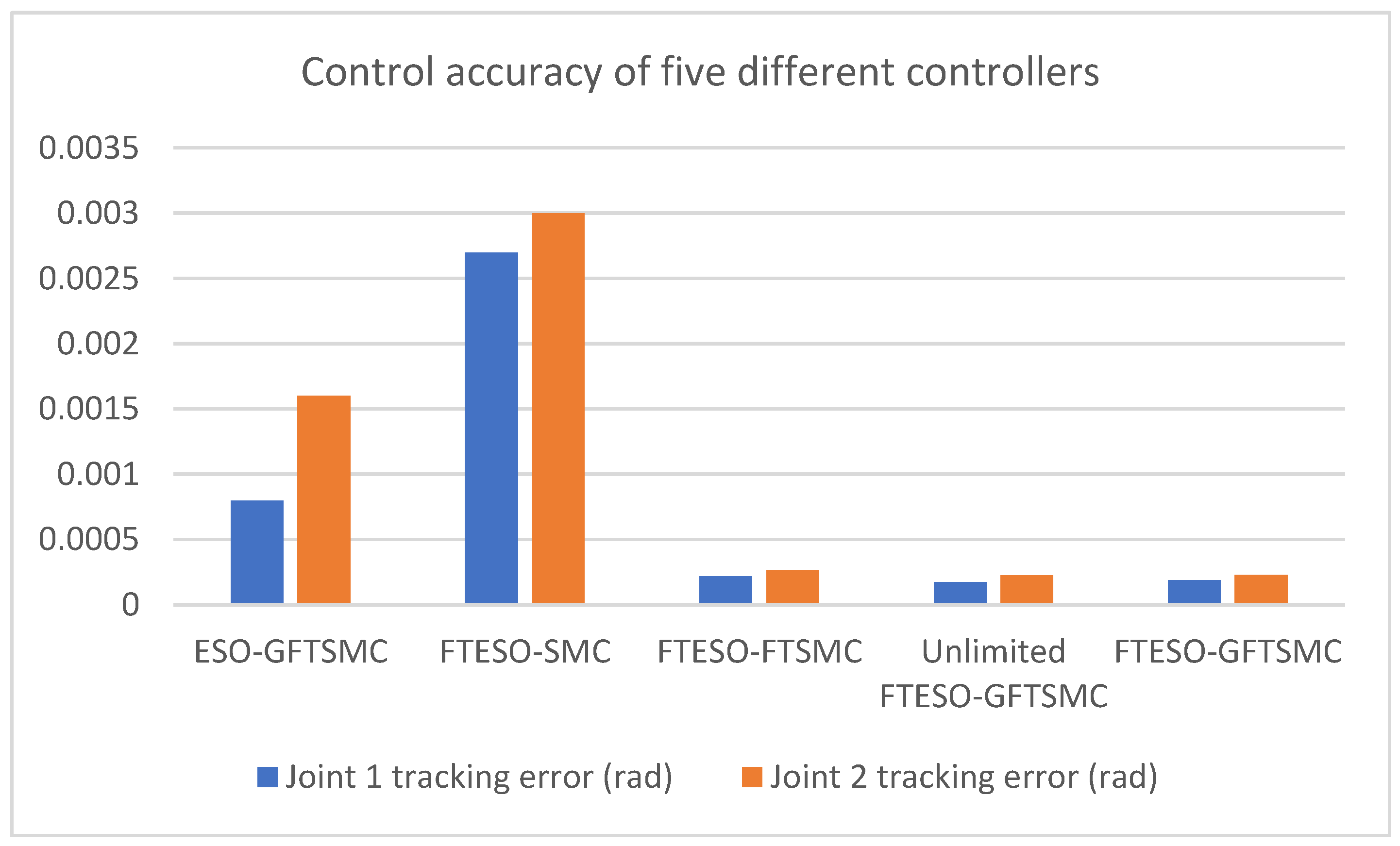
Controller	Joint 1 Tracking Error (Rad)	Joint 2 Tracking Error (Rad)
ESO−GFTSMC	7.98 × 10−4	1.6 × 10−3
FTESO−SMC	2.7 × 10−3	3 × 10−3
FTESO−FTSMC	2.18 × 10−4	2.67 × 10−4
Unlimited FTESO−GFTSMC	1.74 × 10−4	2.25 × 10−4
FTESO−GFTSMC	1.87 × 10−4	2.31 × 10−4

shows the control accuracy of the five controllers, further supporting these conclusions. Figure 9 provides a histogram comparing the control accuracy of the five control schemes.

Figure 10 presents the output torque of the five control methods used in the experiment. From the figure, the initial output torque peak of the FTESO−GFTSMC without output limitation reaches 98.4581 N·m, exceeding the maximum torque of the given actuator and far surpassing the torque required during the control process. In practical control applications, it may damage the actuator, potentially leading to failure in completing the control task. Figure 10 shows the effectiveness of the proposed output limiting component. While enhancing control precision, the controller’s computational load remains a critical factor in underwater vehicle control applications. In the computer simulation experiment (Intel (R) Core (TM) i7-7700HQ CPU @ 2.80 GHz 2.81 GHz processor, 16.0 GB RAM, 64-bit operating system, x64-based processor), the single-step running times of the above five control algorithms were measured as follows: 0.1827 s for ESO+GFTSMC, 0.2044 s for FTESO+SMC, 0.2199 s for FTESO+FTSMC, 0.2150 s for Unlimited FTESO+GFTSMC, and 0.2152 s for FTESO+GFTSMC. These results indicate that the proposed method exhibits only a negligible increase in computational load compared with other advanced control methods.

5. Conclusions

To address the challenge of trajectory-tracking control for underwater manipulators operating in disturbed underwater environments, this study proposed an enhanced dynamic model and designed a global fast terminal sliding mode controller based on a finite-time extended state observer. To mitigate excessive control output variations, the controller implements both output limitation and smoothing mechanisms. Simulation results demonstrated that the proposed finite-time extended state observer achieves superior observation accuracy and effectively provides feedforward compensation for the controller. By combining the FTESO with the global fast terminal sliding mode control, the high-precision trajectory-tracking control of the underwater manipulator is achieved, with the controller successfully constraining the output torque while maintaining the tracking error below 2.4 × 10⁻⁴ rad. The tracking accuracy of the proposed method was improved by 76.57%, 30.74%, and 14.22%, respectively, when compared with ESOGFTSMC, FTESOSMC, and FTESOFTSMC. Due to experimental constraints, this study did not include physical or hardware-in-the-loop (HIL) experiments. Future research will extend to multi-joint underwater manipulator control and parameter optimization. Emphasis will be placed on developing physical validation frameworks encompassing both shallow-water tank experiments and deep-sea robotic platform trials, while implementing a comprehensive evaluation system that integrates tracking performance with engineering metrics such as actuator energy consumption and disturbance recovery time.

References

- Martin, S.C.; Whitcomb, L.L. Nonlinear Model-Based Tracking Control of Underwater Vehicles with Three Degree-of-Freedom Fully Coupled Dynamical Plant Models: Theory and Experimental Evaluation. IEEE Trans. Control Syst. Technol. 2018, 26, 404–414. [Google Scholar] [CrossRef]
- Sivcev, S.; Coleman, J.; Omerdic, E.; Dooly, G.; Toal, D. Underwater Manipulators: A Review. Ocean Eng. 2018, 163, 431–450. [Google Scholar] [CrossRef]
- Pistone, A.; Ludovico, D.; Casareto, L.D.V.M.; Leggieri, S.; Canali, C.; Caldwell, D.G. Modelling and Control of Manipulators for Inspection and Maintenance in Challenging Environments: A Literature Review. Annu. Rev. Control 2024, 57, 100949. [Google Scholar] [CrossRef]
- Wang, R.; Huang, W.; Tang, Y.; Zhang, Z.; Bai, D.; Lv, Y. Global Fast Terminal Sliding Mode Control for Underwater Manipulators Based on Extended State Observer Compensation. In Proceedings of the OCEANS 2024—Singapore, Singapore, 14–17 April 2024. [Google Scholar]
- Venkataramanan, K.; Arun, M.; Jha, S.; Sharma, A. Analyzing Stability and Structural Aspects of Embedded Fuzzy Type 2 PID Controller for Robot Manipulators. J. Intell. Fuzzy Syst. 2024, 46, 1429–1442. [Google Scholar] [CrossRef]
- Silva, F.; Batista, J.; Souza, D.; Lima, A.; dos Reis, L.; Barbosa, A. Control and Identification of Parameters of a Joint of a Manipulator Based on PID, PID 2-DOF, and Least Squares. J. Braz. Soc. Mech. Sci. Eng. 2023, 45, 327. [Google Scholar] [CrossRef]
- Zhou, Y.; He, X.; Shao, F.; Zhang, X. Research on the Optimization of the PID Control Method for an EOD Robotic Manipulator Using the PSO Algorithm for BP Neural Networks. Actuators 2024, 13, 386. [Google Scholar] [CrossRef]
- Hu, Y.; Li, B.; Jiang, B.; Han, J.; Wen, C.-Y. Disturbance Observer-Based Model Predictive Control for an Unmanned Underwater Vehicle. J. Mar. Sci. Eng. 2024, 12, 94. [Google Scholar] [CrossRef]
- Null, W.D.; Edwards, W.; Jeong, D.; Tchalakov, T.; Menezes, J.; Hauser, K. Automatically-Tuned Model Predictive Control for an Underwater Soft Robot. IEEE Robot. Autom. Lett. 2024, 9, 571–578. [Google Scholar] [CrossRef]
- Liu, W.; Xu, J.; Li, L.; Zhang, K.; Zhang, H. Adaptive Model Predictive Control for Underwater Manipulators Using Gaussian Process Regression. J. Mar. Sci. Eng. 2023, 11, 1641. [Google Scholar] [CrossRef]
- Zhong, Y.; Yang, F. Dynamic Modeling and Adaptive Fuzzy Sliding Mode Control for Multi-Link Underwater Manipulators. Ocean Eng. 2019, 187, 106202. [Google Scholar]
- Liu, M.; Tang, Q.; Li, Y.; Liu, C.; Yu, M. A Chattering-Suppression Sliding Mode Controller for an Underwater Manipulator Using Time Delay Estimation. J. Mar. Sci. Eng. 2023, 11, 1742. [Google Scholar] [CrossRef]
- Zaare, S.; Soltanpour, M.R. Uncertainty and Velocity Observer-Based Predefined-Time Nonsingular Terminal Sliding Mode Control of the Underwater Robot Manipulators. Eur. J. Control 2024, 75, 100939. [Google Scholar] [CrossRef]
- Mao, J.; Song, G.; Hao, S.; Zhang, M.; Song, A. Development of a Lightweight Underwater Manipulator for Delicate Structural Repair Operations. IEEE Robot. Autom. Lett. 2023, 8, 6563–6570. [Google Scholar] [CrossRef]
- Ge, D.; Wang, G.; Ge, J.; Xiang, B.; You, Y.; Feng, A. Trajectory Tracking Control of Two-Joint Underwater Manipulator in Ocean-Wave Environment. Ocean Eng. 2024, 292, 116329. [Google Scholar] [CrossRef]
- Liao, L.; Gao, L.; Ngwa, M.; Zhang, D.; Du, J.; Li, B. Adaptive Super-Twisting Sliding Mode Control of Underwater Mechanical Leg with Extended State Observer. Actuators 2023, 12, 373. [Google Scholar] [CrossRef]
- Borlaug, I.L.G.; Gravdahl, J.T.; Sverdrup-Thygeson, J.; Pettersen, K.Y.; Loria, A. Trajectory Tracking for Underwater Swimming Manipulators Using a Super Twisting Algorithm. Asian J. Control 2019, 21, 208–223. [Google Scholar] [CrossRef]
- Wang, Y.; Guan, Y.; Li, H. Observer-Based Finite-Time Sliding-Mode Control of Robotic Manipulator with Flexible Joint Using Partial States. Int. J. Intell. Syst. 2023, 2023, 8859892. [Google Scholar] [CrossRef]
- Fan, Y.; Sun, L.; Bai, X.; Zhao, Y.; Hui, X.; Wang, Y. Trajectory Tracking Control of Underwater Manipulator Based on Adaptive Arctangent Nonsingular Terminal Sliding Mode. Control Decis. 2025, 40, 205–213. [Google Scholar]
- Xue, H.; Huang, J. Dynamic Modeling and Vibration Control of Underwater Soft-Link Manipulators Undergoing Planar Motions. Mech. Syst. Signal Process. 2022, 181, 109540. [Google Scholar] [CrossRef]
- Fu, W.; Wen, H.; Huang, J.; Sun, B.; Chen, J.; Chen, W.; Feng, Y.; Duan, X. Adaptive Sliding Mode Control of Underwater Manipulator Based on Nonlinear Dynamics Model Compensation. J. Tsinghua Univ. (Sci. Technol.) 2023, 63, 1068–1077. [Google Scholar]
- Huang, K.; Wang, Z. Research on Robust Fuzzy Logic Sliding Mode Control of Two-DOF Intelligent Underwater Manipulators. Math. Biosci. Eng. 2023, 20, 16279–16303. [Google Scholar] [CrossRef] [PubMed]
- Zhou, Z.; Tang, G.; Huang, H.; Han, L.; Xu, R. Adaptive Nonsingular Fast Terminal Sliding Mode Control for Underwater Manipulator Robotics with Asymmetric Saturation Actuators. Control Theory Technol. 2020, 18, 81–91. [Google Scholar] [CrossRef]
- Wang, F.; Chao, Z.-Q.; Huang, L.-B.; Li, H.-Y.; Zhang, C.-Q. Trajectory Tracking Control of Robot Manipulator Based on RBF Neural Network and Fuzzy Sliding Mode. Clust. Comput. 2019, 22, 5799–5809. [Google Scholar] [CrossRef]
- Zhu, D.; Yang, S.X.; Biglarbegian, M. A Fuzzy Logic-Based Cascade Control without Actuator Saturation for the Unmanned Underwater Vehicle Trajectory Tracking. J. Intell. Robot. Syst. 2022, 106, 39. [Google Scholar] [CrossRef]
- Dao, P.N.; Dang, N.T.; Nguyen, T.L.; Dinh, G.K. Finite-Time Sliding Mode Control Strategies for Perturbed Input-Constrained Nonlinear Bilateral Teleoperation Systems with Variable-Time Communication Delays. Intell. Serv. Robot. 2025, 18, 363–378. [Google Scholar] [CrossRef]
- Zhao, Z.; Li, T.; Cao, D.; Yang, J. Bilateral Continuous Terminal Sliding Mode Control for Teleoperation Systems with High-Order Disturbances. Nonlinear Dyn. 2023, 111, 5345–5358. [Google Scholar] [CrossRef]
- Liu, X.; Wei, C.; Shan, Z.; Shan, Z.; Liu, Y. Trajectory Tracking Control of Unmanned Vehicles with Odometer Positioning Compensation Based on Extended State Observer. Chin. J. Sci. Instrum. 2024, 45, 313–320. [Google Scholar]
- Wang, N.; Zhu, Z.; Qin, H.; Deng, Z.; Sun, Y. Finite-Time Extended State Observer-Based Exact Tracking Control of an Unmanned Surface Vehicle. Int. J. Robust Nonlinear Control 2021, 31, 1704–1719. [Google Scholar] [CrossRef]
- Perruquetti, W.; Floquet, T.; Moulay, E. Finite−Time Observers: Application to Secure Communication. IEEE Trans. Autom. Control 2008, 53, 356–360. [Google Scholar] [CrossRef]
- Bhat, S.P.; Bernstein, D.S. Geometric Homogeneity with Applications to Finite−Time Stability. Math. Control Signals Syst. 2005, 17, 101–127. [Google Scholar] [CrossRef]
- Nie, J.; Wang, H.; Lu, X.; Lin, X.; Sheng, C.; Zhang, Z.; Song, S. Finite-Time Output Feedback Path Following Control of Underactuated MSV Based on FTESO. Ocean Eng. 2021, 224, 108660. [Google Scholar] [CrossRef]
- Hardy, G.H.; Littlewood, J.E.; Pólya, G. Inequalities (Cambridge Mathematical Library); Cambridge University Press: Cambridge, UK, 1934. [Google Scholar]
- Song, Z.; Li, H.; Sun, K. Finite−time control for nonlinear spacecraft attitude based on terminal sliding mode technique. ISA Trans. 2013, 53, 117–124. [Google Scholar] [CrossRef] [PubMed]
- Fu, M.Y.; Wang, Q.S. Safety−Guaranteed, Robust, Nonlinear, Path−Following Control of the Underactuated Hovercraft Based on FTESO. J. Mar. Sci. Eng. 2023, 11, 1235. [Google Scholar] [CrossRef]