Article

Multi-Objective Optimization Based on Response Surface Methodology and Multi-Objective Particle Swarm Optimization for Pipeline Selection of Replenishment Oiler

1
State Key Laboratory of Ocean Engineering, Shanghai Jiao Tong University, Shanghai 200240, China
2
Institute of Power Plants and Automation, Shanghai Jiao Tong University, Shanghai 200240, China
3
Marine Design & Research Institute of China, Shanghai 200011, China
*
Author to whom correspondence should be addressed.
J. Mar. Sci. Eng. 2025, 13(6), 1037; https://doi.org/10.3390/jmse13061037
Submission received: 27 April 2025 / Revised: 17 May 2025 / Accepted: 22 May 2025 / Published: 25 May 2025
(This article belongs to the Section Ocean Engineering)

Abstract

:
Ship pipeline selection, as a crucial component of ship pipeline design, is often a time-consuming process due to its high complexity. In this study, the response surface methodology combined with the multi-objective particle swarm optimization algorithm was used to optimize the fuel pipeline resistance and its space volume, aiming to select the optimal design scheme for an X-type replenishment oiler. Firstly, a one-dimensional pipeline system simulation model of a replenishment oiler was established based on the Flowmaster software (version 4.2_0 2020), and the fueling process was simulated. The simulation results were validated against the experimental results, and good agreements were obtained. Then, the response surface methodology was employed to establish regression models for the pipeline resistance, pipeline space volume, and imbalance degree of branch flows. Finally, multi-objective particle swarm optimization was used to optimize the target and select the optimal virtual solution from the Pareto front. Constrained by the international application standard, the optimal real solution was determined. Compared with the original scheme, the optimized scheme reduced the resistance by 3.57% for the #1 pipeline system and by 3.51% for the #2 pipeline system, respectively, and the space volume of the pipeline system was reduced by 5.72% while ensuring the flow balance.

1. Introduction

The globalization of trade has contributed to a booming shipping industry. Studies show that marine transportation accounts for about 80% or more of international trade and is still growing [1,2]. Booming maritime economics have contributed to the development of the shipbuilding industry [3]. Nowadays, ship construction is a complicated compound of art and science, especially for ship pipeline design (SPD) [4]. The primary objective of SPD is to deliver a reliable and durable pipeline system while minimizing the consumption of high-cost materials and installation resources [5], and it generally includes pipeline layout and selection. For mature commercial ships, pipeline selection often relies on the designer’s experience and database. However, for special ships, a lack of design experience can pose great challenges in pipeline selection and can also affect the realization of a ship’s function. Replenishment oilers, unlike normal cargo ships, are designed to address the modern replenishment requirements for oil and other liquid substances for offshore operations, especially to provide reliable fuel support to vessels and facilities far from land. These facilities do not return to port bases for replenishment due to special maritime operational missions [6]. Therefore, material replenishment is carried out by replenishment oilers, which require a high fuel storage capacity and a high fuel replenishment efficiency. In addition, most of the supply process requires that the flow between different supply ports should be as similar as possible to prevent local equipment overload. Accordingly, pipeline design for replenishment oilers has become more crucial, and it needs to ensure minimal resistance, a low weight, and a balanced flow rate at different supply ports as much as possible. Reducing the resistance of pipeline systems is conducive to improving fuel replenishment efficiency and saving on replenishment time, and decreasing the pipeline weight can save more space for storing oil and improve replenishment endurance at sea. Hence, pipeline selection is an important task in the SPD of replenishment oilers.
As the main way of transporting liquids or gases in ships, pipelines are known as the “blood vessel of the ship”, and their significance is self-evident [7,8]. Researchers have paid much attention to ship pipeline design [9]. Due to limited space in the ship’s cabin, the pipeline route needs to be scheduled [10]. However, due to the high complexity of pipeline design, engineers usually use drawing software to construct basic drawings and then combine their experience to complete pipeline layouts and selections [11]. Nevertheless, due to the complexity and diversity of ship pipeline system functions, it is often difficult to satisfy the design requirements only based on experience. For example, the hull structure and the layout of the ship equipment will affect the direction of the pipeline route. Furthermore, the functions and performance requirements of the pipeline system will also influence the selection of pipeline parameters. This interdependency necessitates iterative redesign cycles, which account more than 50% of the total design time in the vessel design phases [12]. With the development of computers and intelligent algorithm technology, more researchers have started taking advantage of professional software and intelligent algorithms to proceed with pipeline design. Zhang et al. [13] developed a layout method integrating a bidirectional guidance mechanism and layering concept, subsequently validating the methodology’s practicality through standardized testing involving diverse marine vessel compartment configurations from practical engineering scenarios. Based on the multi-objective optimization algorithm, Lin et al. [14] introduced a multi-objective collaborative particle swarm optimization algorithm based on mixed dimensions, implementing it in a real ship’s cabin pipeline system to obtain an enhanced engineering pipeline arrangement scheme. However, for a specialized pipeline design, a single algorithm may require more work to ensure the desirable design results. Ha et al. [15] proposed an intelligent ship pipe routing design method integrating a dual-core knowledge model with pathfinding algorithms. They compared the results with manual design results, which showed that the proposed method could obtain a preferable pipeline system design. Wang et al. [16] introduced an enhanced ant colony optimization framework incorporating collaborative human–machine interaction, with numerical simulations validating its functional robustness and optimization capability in complex ship engineering scenarios. In order to accelerate the pathfinding speed, Min et al. [17] developed a modified jump point search (JPS) algorithm for the pipeline layout, and the results showed that the improved jump point search algorithm could obtain a faster pathfinding speed in complex maritime engineering environments.
Even though there has been great progress in pipeline design in the literature, most studies have only focused on the pipeline layout for mature ships with rich design experience, omitting the pipeline selection. In the actual design of a special ship’s pipeline system, such as replenishment oilers, the selection of pipeline parameters is also an important section, affecting the pipeline transportation performance and impacting the subsequent pipeline layout. Moreover, the present literature is mostly concerned with the pipeline layout inside ship cabins without addressing the design of the ship deck pipeline system. However, ship deck pipelines are very long, contributing to a large proportion of the resistance, material weight, and flow balance. Because of the special function of a replenishment oiler, its deck pipeline system design should not be neglected. In addition, unlike the cabin environment, the ship deck is not subjected to strict spatial constraints, and the pipeline layouts can be ignored. Therefore, the priority in the deck pipeline design of replenishment oilers is to develop a good selection program that not only reduces weight but also reduces resistance to improve the efficiency of the fuel recharge. Therefore, focusing on an X-type replenishment oiler, this study combines machine learning methods with multi-objective optimization algorithms to determine the optimal pipeline selection. In this paper, machine learning (response surface methodology, RSM) and intelligent algorithms (multi-objective particle swarm optimization, MOPSO) are used for pipeline selection for special ships, which provides a new method for pipeline design. The proposed RSM-MOPSO optimization framework enables the rapid generation of pipeline system configuration recommendations for specialized vessels, effectively supporting engineers in conducting pipeline design tasks. This approach addresses a critical research gap in methodological studies for pipeline selection within ship engineering.
The paper is organized as follows: in Section 2, a fuel transportation pipeline system is established and verified against experimental data. Then, in Section 3, a regression equation of the fuel transportation pipeline system is constructed based on RSM, and analysis of variance (ANOVA) of the regression equation is performed. Section 4 introduces the multi-parameter and multi-objective optimization based on the MOPSO algorithm, and optimal parameter design is obtained. Finally, the main conclusions of this study are drawn in Section 5.

2. Methodology

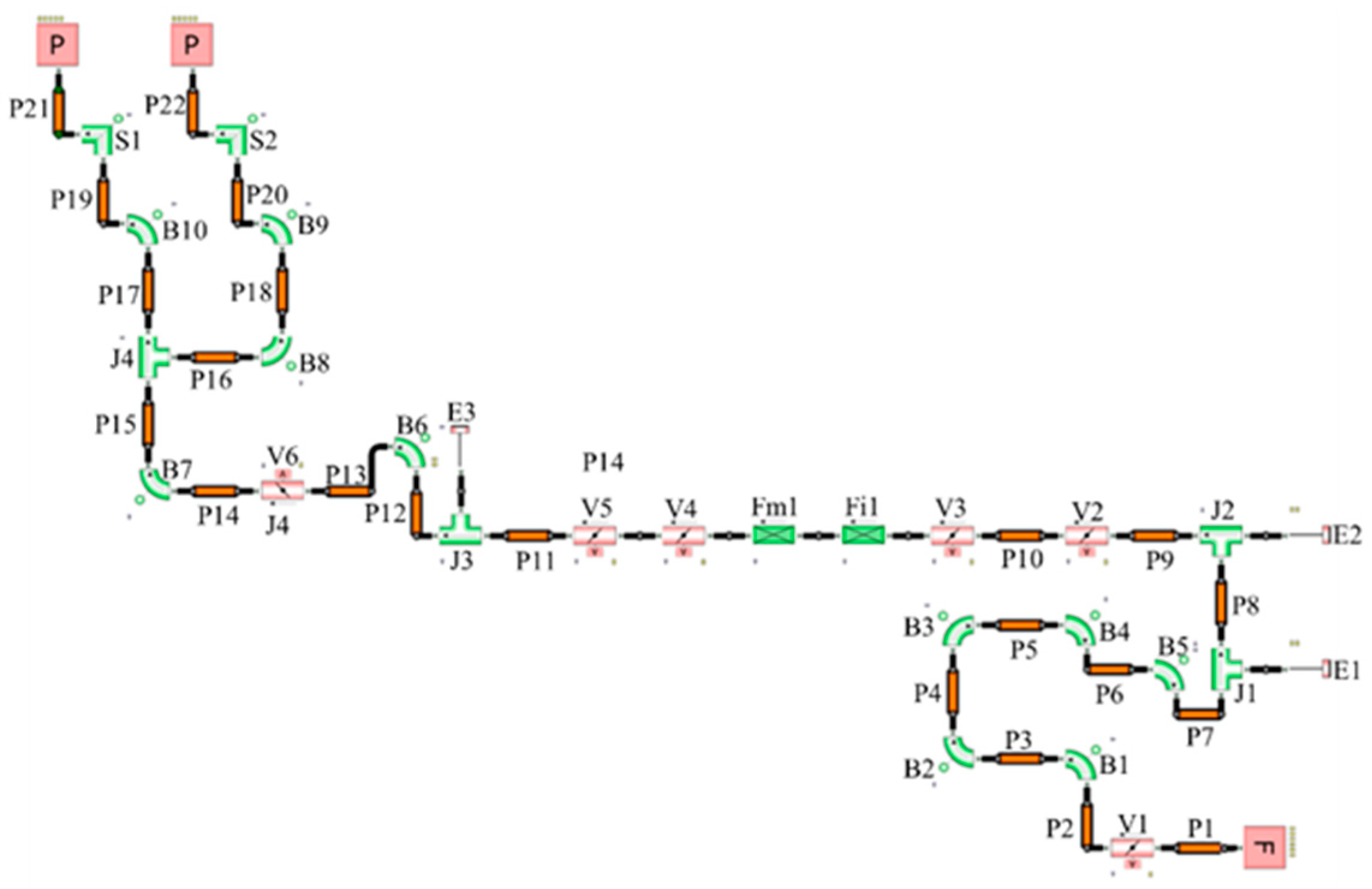
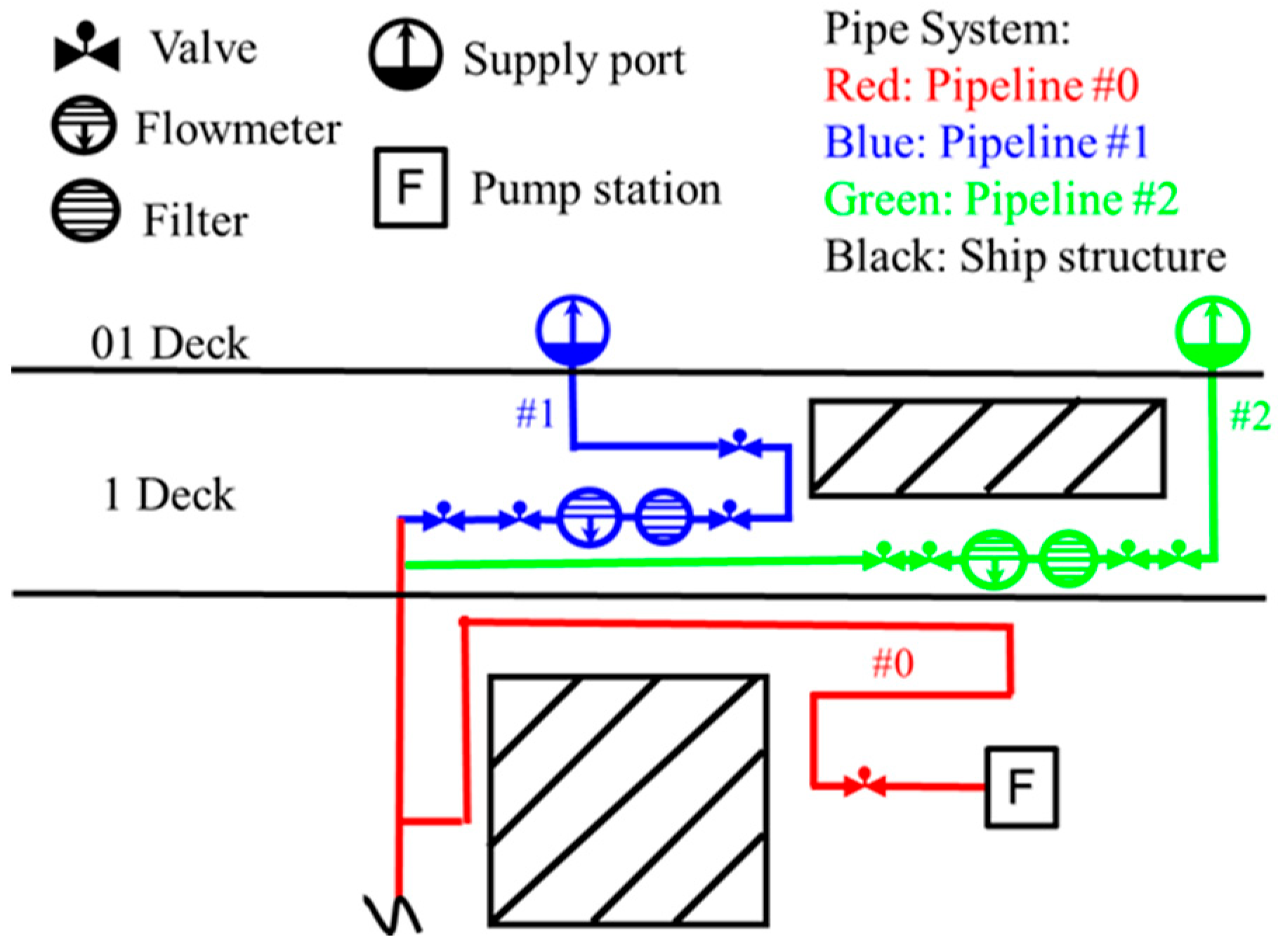
2.1. Problem Description

Figure 1 shows a schematic diagram of a deck refueling pipeline system for an X-type replenishment oiler. It can be seen that the pipeline system mainly consists of three parts, including main oil pipeline #0 (red) and deck refueling pipelines #1 (blue) and #2 (green). The oil is first pumped from the pump station into the main oil pipe (#0) and then diverted through the #1 and #2 branches to reach the supply port to complete the external refueling. The following parameters are involved in pipeline selection: The pipe diameters of main oil pipeline #0 and deck refueling pipelines #1 and #2, which are represented by D0, D1, and D2, respectively. The bend–diameter ratios (R/D) of the pipeline are characterized by R0, R1, and R2. The resistance forces of the external refueling #1 and #2 pipeline systems are expressed as Y1 and Y2. The pipeline volume of the entire system is expressed as Y3. The flow imbalance between the two refueling stations is termed as Y4. The supply process was simulated by the Flowmaster software, and the dependent variables Y1, Y2, and Y4 were obtained. Y3 was calculated based on the selected pipe and bend parameters, assuming their occupied cylindrical volume, as expressed in Equation (1).
V b e n d = n i π d i / 2 2 1 4 π R i R i = R i / d i V p i p e = π D i 2 2 L i Y 3 = 0 2 V b e n d , i + V p i p e , i , i = 0 , 1 , 2
where V b e n d and V p i p e are the bend and pipe volumes, respectively; n is the number of bends; d i is the bend diameter; R i is the bend radius; R i is the bend–diameter ratio; D i is the pipe diameter; and L i is the pipe length. Y4 is expressed as per Equation (2).
Y 4 = F 1 F 2 F 1 100 %
where F 1 and F 2 are the flow of supply ports #1 and #2, respectively.
According to the special ship design specifications, each branch of the system should have a minimum resistance and space volume, and two branches should satisfy the flow balance [18]. Therefore, this is a multi-objective optimization problem, and the mathematical equation is formulated as per Equation (3).
min Y 1 min Y 2 min Y 3 Y 4 5 %

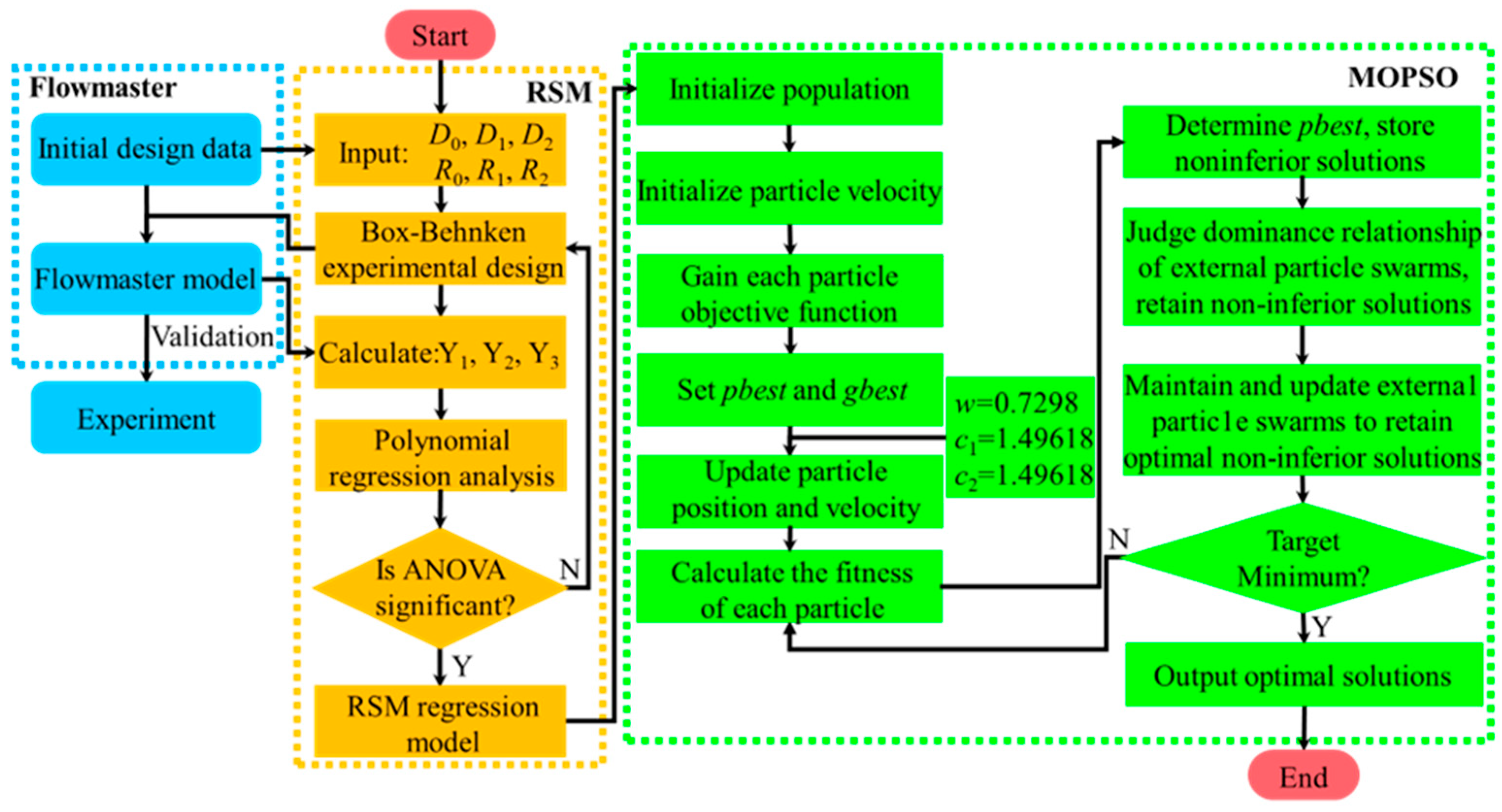
2.2. Response Surface Methodology

Response surface methodology (RSM) serves as a computational optimization framework that utilizes statistical regression analysis to construct predictive models, mapping the interdependencies between input variables and system outputs. Widely used in engineering design, this technique enables the explanation of complex multivariate relationships through planned experimental designs, significantly reducing required tests while preserving analytical precision [19,20]. In this study, RSM was used to analyze the effect of the pipe diameters and bend–diameter ratio on the pipeline resistance and the space volume. Usually, the interdependency between the design variables and the system response can be captured by Equation (4).
f = a 0 + i = 1 n a i x i + i = 1 n j = 1 , i < j n a i j x i x j + i = 1 n a i i x i 2 + c
where f is the predicted output, including Y1, Y2, Y3, and Y4; x is the optimization parameter, covering the pipe diameter and bend–diameter ratio; n is the number of variables; c represents the residual error between approximations; and a is the model coefficient of each order.
Once a regression model has been established, the predictive performance of the RSM model needs to be systematically assessed. According to the statistical metrics, a significance check is used to evaluate the predictive ability of the response surface model, and the judgment criteria are calculated based on Equations (5)–(7). Specifically, the determination coefficient ( R 2 ), defined in Equation (5), is introduced to explain the variability in the data.
R 2 = 1 S S r e s i d u a l S S r e s i d u a l + S S model
R 2 should be greater than 0.8 in the engineering field [21]. Although R 2 is a commonly used metric for assessing a model’s fit, it tends to increase with the addition of more predictors, even if those predictors lack real predictive power. To overcome this shortcoming, the adjustment coefficient ( R A d j . 2 ) introduces a penalty factor that accounts for both the number of predictors and the sample size. This adjustment mechanism effectively suppresses the R A d j . 2 enlargement caused by irrelevant predictors while retaining the ability to detect model validity. R A d j . 2 for the regression model is formulated as per Equation (6).
R A d j . 2 = 1 S S r e s i d u a l d f r e s i d u a l / S S r e s i d u a l + S S model d f r e s i d u a l + d f model
This R A d j . 2 reflects the overall strength of the relationship between the independent and dependent variables, and a value closer to 1.0 indicates a stronger correlation [22]. The prediction degree coefficient ( R Pred . 2 ) is often used to validate the generalization performance and evaluate the ability of the model to predict new data. R Pred . 2 for the RSM model can be written as per Equation (7).
R Pred . 2 = 1 S S p r e d i c t e d S S r e s i d u a l + S S model
The closer the value of R Pred . 2 is to 1.0, the more reliable the predictive model is. To maintain model robustness and prevent overfitting risks, the difference between R Pred . 2 and R A d j . 2 should be controlled within 0.2 [23]. In the RSM model, S S represents the quadratic sum, S S p r e d i c t e d is the sum of the squared prediction error, and d f represents the degrees of freedom.

2.3. MOPSO Algorithm

Engineering optimization problems inherently involve multi-objective formulations with complex trade-offs between competing parameters. These objectives typically exhibit nonlinear interdependencies, and it is difficult to achieve a single solution that optimizes all objectives concurrently [24,25,26]. The Pareto frontier scheme has emerged as a principal methodology for such cases [27,28,29]. Within the Pareto frontier framework, non-dominated solutions, which are termed as the Pareto-optimal solutions, exhibit mutual non-dominance, characterized by two axiomatic properties: (1) solutions within the frontier strictly dominate external alternatives; and (2) inter-solution comparisons within the Pareto-optimal set inherently exhibit mutual non-comparability of solution superiority [30]. As a population-based metaheuristic in computational intelligence optimization algorithms, particle swarm optimization (PSO) has demonstrated prominent applicability in multi-objective optimization scenarios due to its computationally efficient architecture and rapid convergence characteristics [31]. Pipeline selection is a multi-objective optimization problem, since it involves three objective variables, Y1, Y2, and Y3. The multi-objective particle swarm optimization (MOPSO) algorithm proposed by Coello et al. [32] was induced in this study because the simple PSO algorithm cannot solve multi-objective optimization problems. The MOPSO algorithm updates the particles in each iteration by tracking the individual and population extremes with a fitness function to calculate the particles’ fitness values. As the particles adjust their positions, their fitness values are recalibrated in real time and compared against personal best and global best archives, enabling the identification of non-dominated solutions through competitive analysis [32,33]. In order to better control the algorithm’s searchability and convergence, the MOPSO algorithm with a weight factor [34] was used in this study. The particle motion for iteration (t + 1) is calculated as per Equation (8) [35].
x i t + 1 = x i t + v i t + 1 v i t + 1 = ω × v i t + c 1 r 1 × p b e s t i t x i t + c 2 r 2 g b e s t t x i t
where i = 1 , 2 , 3 n represents the index particle; x i represents the location of the i-th particle at the i-th iteration; v i represents the velocity of the i-th particle at the i-th iteration; g b e s t represents the global optimal location; p b e s t represents the optimal location of the i-th particle found so far; ω represents the weight factor of the particle; c 1 and c 2 represent the acceleration factor; and r 1 and r 2 represent a random value that is uniformly distributed in the interval [0, 1] [36]. ω is decisive for the convergence of the algorithm: when ω > 1, the particle velocity grows exponentially with time, which triggers the system to diverge, whereas ω < 0 will cause the velocity to decay to a stagnant state. In addition, more prominent acceleration factors ( c 1 , c 2 ) cause the velocity to explode to a large value quickly. Both the weight factor ( ω ) and acceleration factors ( c 1 , c 2 ) will affect the algorithm’s convergence [37,38]. Eberhart et al. [39] showed that the algorithm converged well when the weight factor ω = 0.7298 and the acceleration factor c 1 = c 2 = 1.49618 (For the sensitivity analysis of parameters, see Appendix A for details.). In summary, the parameters of the MOPSO algorithm used in this study were set as follows: the population size was 100, the maximum number of iterations was 100, the weight factor ω = 0.7298, and the acceleration factor c 1 = c 2 = 1.49618. In this work, a 1D simulation model was developed based on the original design. The simulation model was calibrated by real ship pipeline replenishment data from a shipyard. The decision variables included D0, D1, and D2 and R0, R1, and R2, with Y1, Y2, and Y3 as the target variables. The design of the experiments incorporating multiple variables was conducted using the Design-Expert 13.0 software, resulting in the selection of 54 representative test configurations. These cases were subsequently simulated using the Flowmaster software to obtain the relevant outputs. A polynomial nonlinear regression model was established through RSM to characterize the relationships between the independent and dependent variables. The MOPSO algorithm with weight was used for optimization to obtain a Pareto optimal solution, with the minimum pipeline resistance and volume as the objectives and the flow imbalance as the constraints. Several optimization cases were analyzed in detail from the Pareto front to determine the optimal solution. The comprehensive optimization framework is summarized in Figure 2.

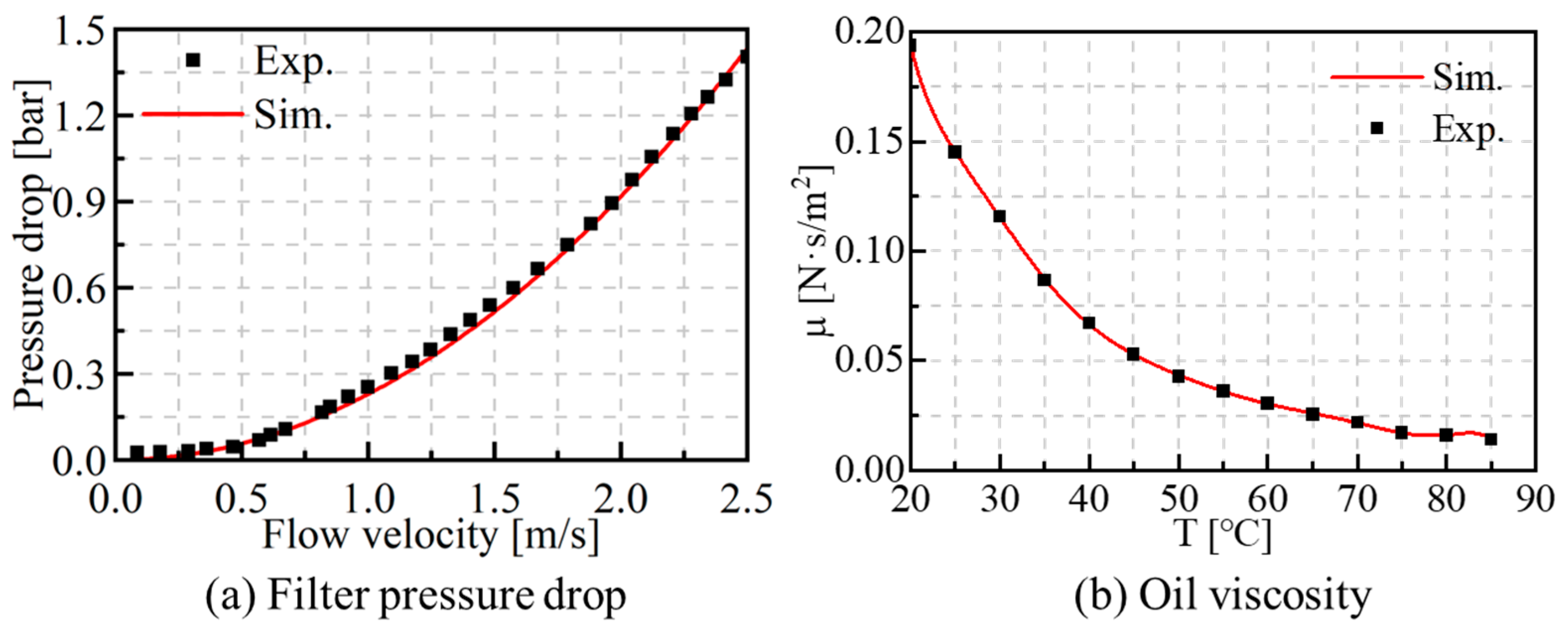
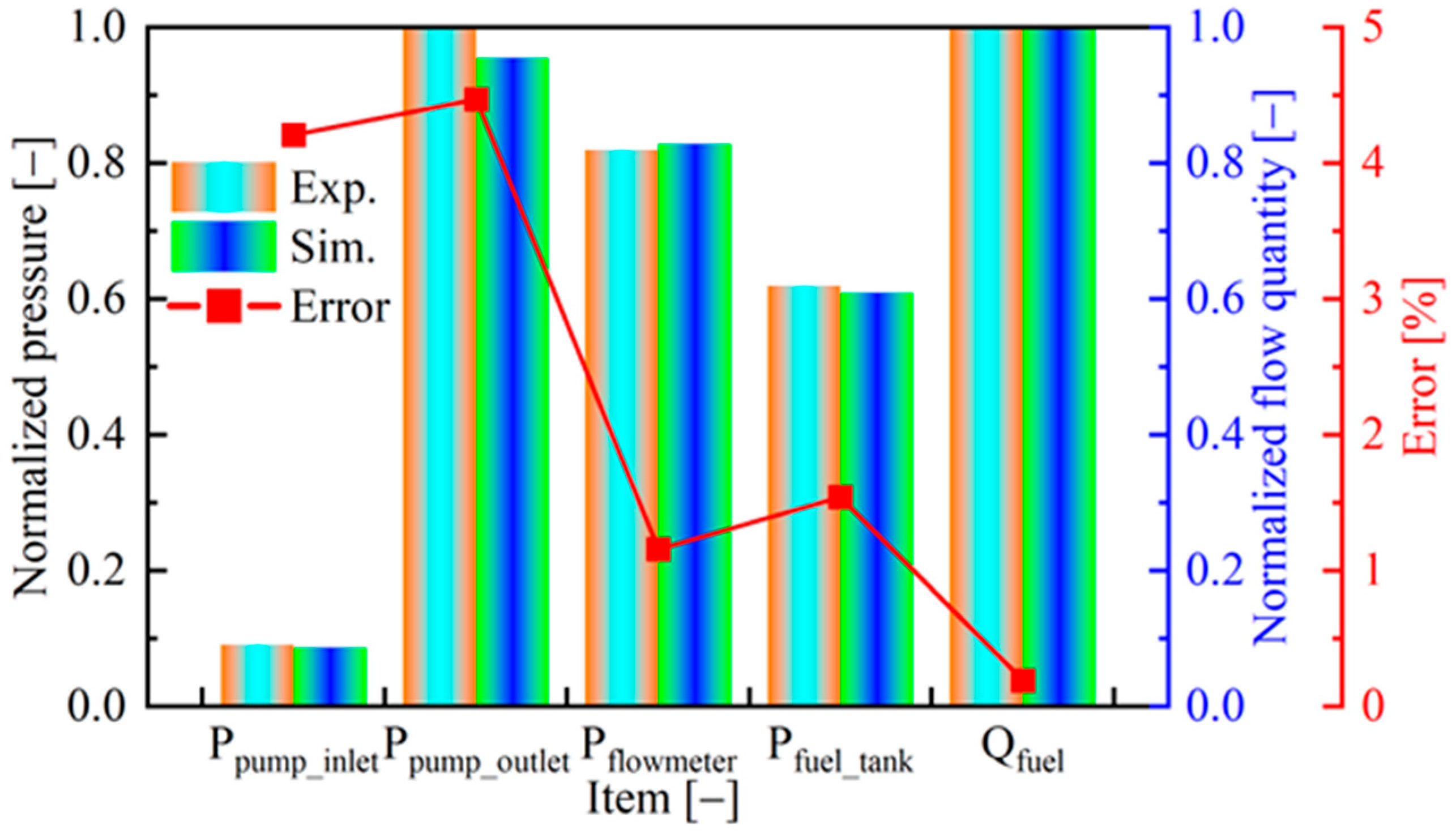
2.4. Establishment and Calibration of Simulation Model

In the Flowmaster software (version 4.2_0 2020), the pressure loss ( h p ) for a circular pipe is calculated as per Equation (9).
h p = f t L v 2 g D
where L is the length of the pipe; D is the diameter of the pipe; g is the acceleration due to gravity; v is the flow velocity inside the pipe; and f t is the along-track loss coefficient, which is specifically calculated by the Colebrook–White equation, as per Equation (10).
f t = 0.25 log k 3.7 D + 5.74 Re 0.9 2
where k is the pipe roughness and Re is the Reynolds number. The pressure loss of the valve ( h v ) is written as per Equation (11).
h v = λ c Re ρ v 2 2
where λ is the flow loss coefficient; c Re is the Reynolds number correction coefficient; and ρ is the fluid density. Based on the above theory, a 1D simulation model was established using the Flowmaster software. Combined with the pipeline layout shown in Figure 1, the 1D simulation model in the Flowmaster software is shown in Figure 3.
Since the pipeline system studied in this research is still in the design stage, there were no available experimental data. Therefore, this work applied the same numerical settings to establish a 1D simulation model for a completed A-type replenishment oiler, aiming to illustrate the reasonability of the numerical settings in the Flowmaster model. As shown in Figure 4, the basic schematic diagram of the A-type replenishment oiler used the #d-1 supply port for external refueling.
Based on the measured data of the A-type replenishment oiler from the shipyard, the simulation results were validated, as shown in Figure 5. Herein, the back pressure of the #d-1 supply port was 2.8 bar, and the external refueling was performed by the No. ④ oil pump. The flow rate at the refueling station was 0.998 (normalized value) when the backflow valve opening degree was 3%. In this study, both the pressure drop of the filter and the oil viscosity were validated, and good agreements were obtained, as presented in Figure 5. Figure 6 shows a comparison of the pressure at different equipment points between the simulation results and the experimental data. As can be seen, the present simulation model could accurately predict the refueling process, including the pressure variation across the pump, flowmeter, and oil tank. The prediction error was within the range of 0.19–4.44%, and the maximum error was obtained for the pump outlet pressure. This may have been due to the fact that the simulation did not consider the resistance of the rappelling pipe near the pump, which resulted in an underestimation of the local along-pipeline loss. Overall, the prediction error for the system was less than 5%, indicating that the present model can be used for further research.

3. RSM Prediction Model

3.1. Model Parameters

According to the RSM modeling theory described in Section 2.2, the Design-Expert 13.0 software was used to establish the response surface alternative model of the refueling pipeline system. Based on the pipeline design demands, the pipe diameter and bend ratios should be in the following range: D0 ∈ [0.293, 0.437], D1, D2 ∈ [0.208, 0.310], R0, R1, R2 ∈ [1, 3]. Combining the Flowmaster and Design-Expert simulation results, the resistance of the external refueling pipeline #1 and #2 obtained from the RSM model can be written as per Equations (12) and (13), respectively.
Y 1 = 23.59167 37.43461 D 0 24.66997 D 1 32.83033 D 2 0.239773 R 0 0.154261 R 1 0.021024 R 2 + 0.019063 D 0 D 1 2.07312 D 1 D 2 + 0.328967 D 0 R 0 0.000087 D 0 R 0 0.000139 D 0 R 2 + 13.36313 D 1 D 2 + 4.08541 × 10 14 D 1 R 0 + 0.257684 D 1 R 1 + 0.035123 D 1 R 2 + 2.5 × 10 5 D 2 R 0 + 0.022941 D 2 R 1 + 0.0706 D 2 R 2 1.25 × 10 6 R 0 R 1 1.25 × 10 6 R 0 R 2 + 0.001624 R 1 R 2 + 42.61207 D 0 2 + 31.93457 D 1 2 + 48.32185 D 2 2 + 0.022022 R 0 2 + 0.015463 R 1 2 0.003531 R 2 2
Y 2 = 23.67834 37.37168 D 0 23.37819 D 1 34.78775 D 2 0.240651 R 0 0.146951 R 1 0.021234 R 2 + 0.019063 D 0 D 1 2.19669 D 0 D 2 + 0.328967 D 0 R 0 0.000087 D 0 R 1 0.000156 D 0 R 2 + 13.84804 D 1 D 2 + 6.52356 × 10 14 D 1 R 0 + 0.242782 D 1 R 1 + 0.033186 D 1 R 2 + 0.000025 D 2 R 0 + 0.022819 D 2 R 1 + 0.074902 D 2 R 2 1.25 × 10 6 R 0 R 1 1.25 × 10 6 R 0 R 2 + 0.001528 R 1 R 2 + 42.56687 D 0 2 + 29.66423 D 1 2 + 51.33763 D 2 2 + 0.022242 R 0 2 + 0.014898 R 1 2 0.00367 R 2 2
The pipeline volume of the entire system (Y3) obtained from the RSM model can be expressed as per Equation (14).
Y 3 = 3.10658 11.83629 D 0 5.95859 D 1 1.98651 D 2 0.705942 R 0 0.252336 R 1 0.084104 R 2 + 0.003745 D 0 D 1 + 0.002723 D 0 D 2 + 2.99692 D 0 R 0 0.000035 D 0 R 1 0.000035 D 0 R 2 0.000481 D 1 D 2 0.000025 D 1 R 0 + 1.50903 D 1 R 1 + 0.000245 D 1 R 2 + 0.000221 D 2 R 0 + 0.000172 D 2 R 1 + 0.502929 D 2 R 2 + 2.38854 × 10 16 R 0 R 1 1.25 × 10 6 R 0 R 2 + 0.000013 R 1 R 2 + 61.9456 D 0 2 + 25.92005 D 1 2 + 44.60838 D 2 2 5.27778 × 10 6 R 0 2 + 4.30556 × 10 6 R 1 2 9.86111 × 10 6 R 2 2
The flow imbalance between the two supply ports (Y4) obtained from the RSM model can be calculated as per Equation (15).
Y 4 = 23.37711 + 16.91295 D 0 + 342.05419 D 1 521.13033 D 2 0.215917 R 0 + 1.8627 R 1 0.070387 R 2 + 6.25559 × 10 12 D 0 D 1 32.88783 D 0 D 2 0.123396 D 0 R 0 + 0.246791 D 0 R 1 0.002307 D 0 R 2 + 128.94351 D 1 D 2 + 4.03757 × 10 13 D 1 R 0 3.95577 D 1 R 1 0.50811 D 1 R 2 + 2.09022 × 10 15 D 2 R 0 0.042343 D 2 R 1 + 1.15791 D 2 R 2 + 0.017769 R 0 R 1 + 2.93828 × 10 16 R 0 R 2 0.025581 R 1 R 2 12.71033 D 0 2 600.91957 D 1 2 + 803.12389 D 2 2 + 0.054874 R 0 2 0.159576 R 1 2 0.034829 R 2 2

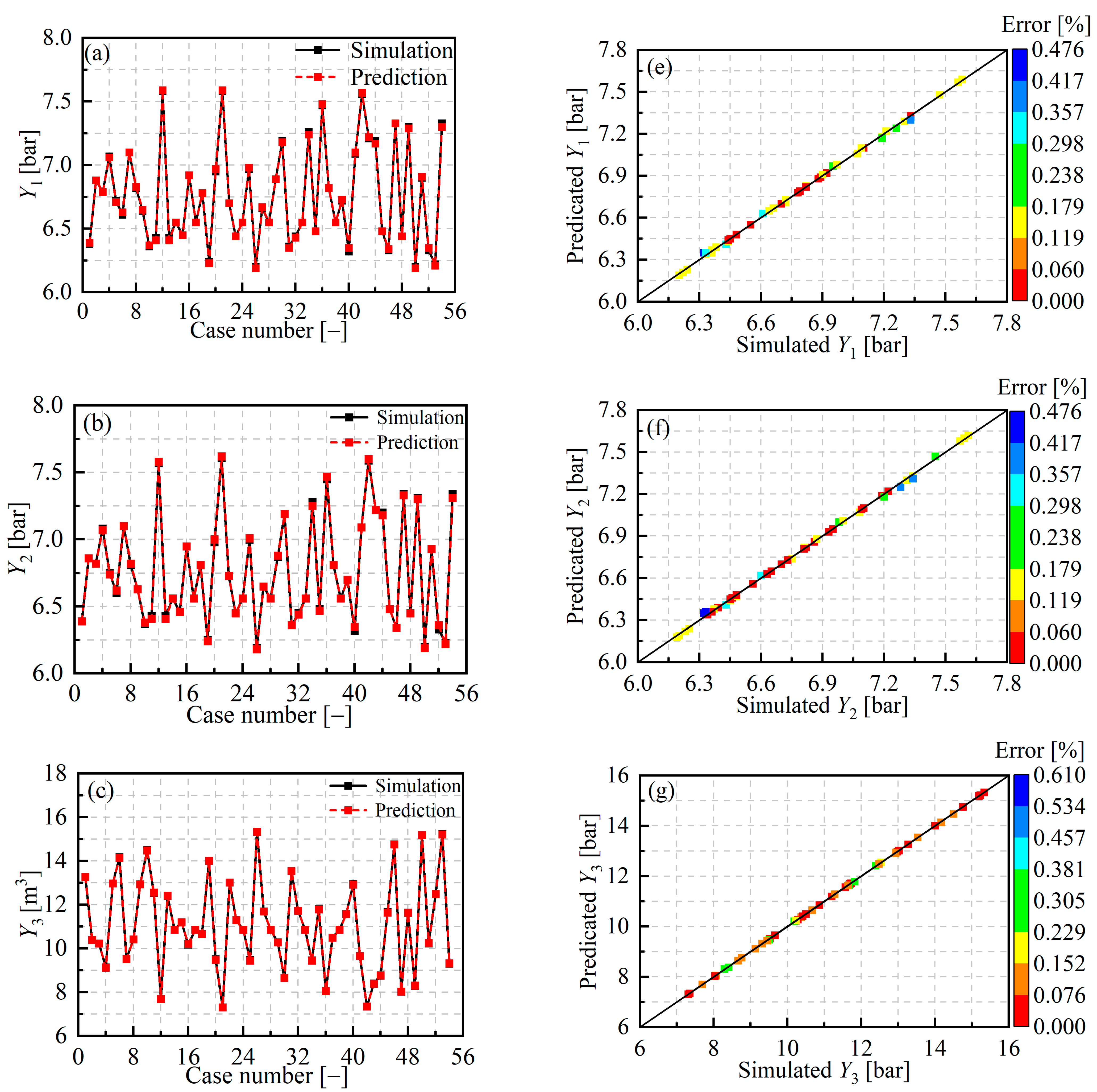
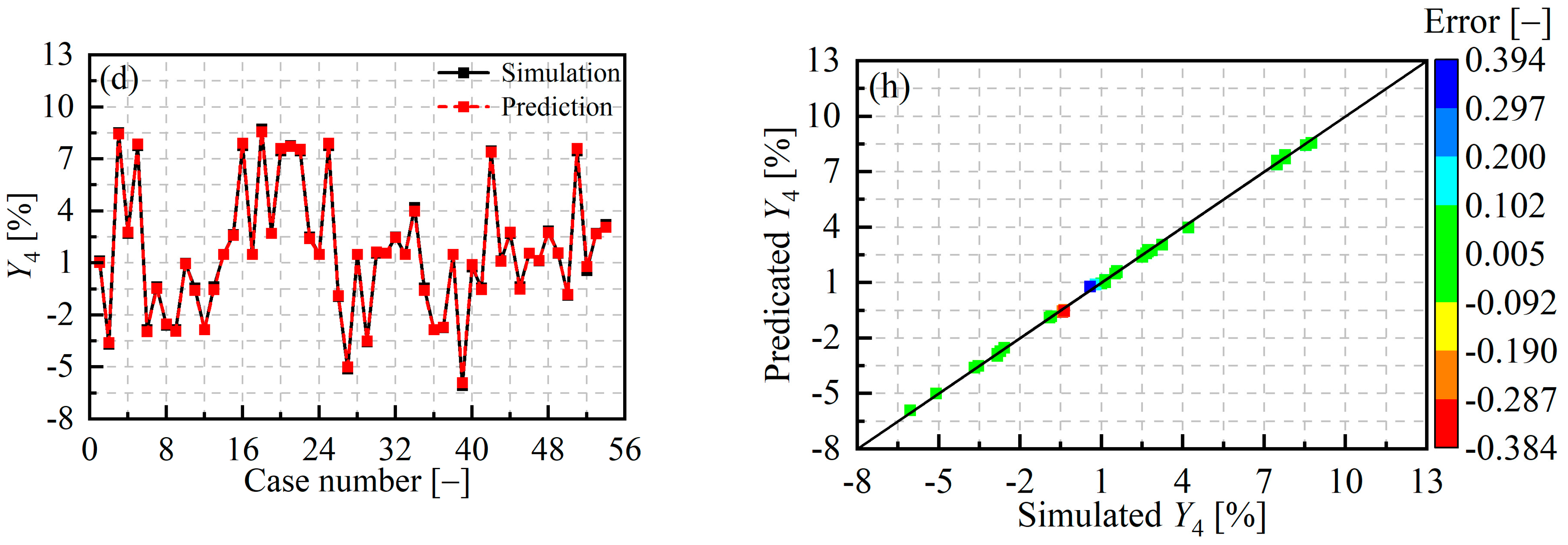
3.2. Predictive Performance

Table 1 lists the ANOVA data of Y1, Y2, Y3, and Y4. The model’s goodness of fit, as indicated by the goodness of fit ( R 2 ), adjusted goodness of fit ( R A d j . 2 ), and predictive power ( R Pr e d . 2 ), was positively correlated with its predictive accuracy. As can be seen from Table 1, all the R 2 values of the prediction models were more significant than 0.98, indicating a high prediction ability [40,41,42], and this means that the model can be used in the following investigation.
In order to visualize the accuracy of the prediction model, its values were compared with the Flowmaster simulation results, and the results are shown in Figure 7. As can be seen, the RSM regression prediction model demonstrated strong agreement with the numerical simulations. In addition, based on the regression curve, it can be observed that the predicted values and the simulation results were very close, which were all located near the regression line. Therefore, it can be concluded that the present RSM model performed very well in predicting the small-sample regression problems for Y1, Y2, Y3, and Y4, and it can be used as an alternative model to optimize the calculations [43].

4. Results and Discussion

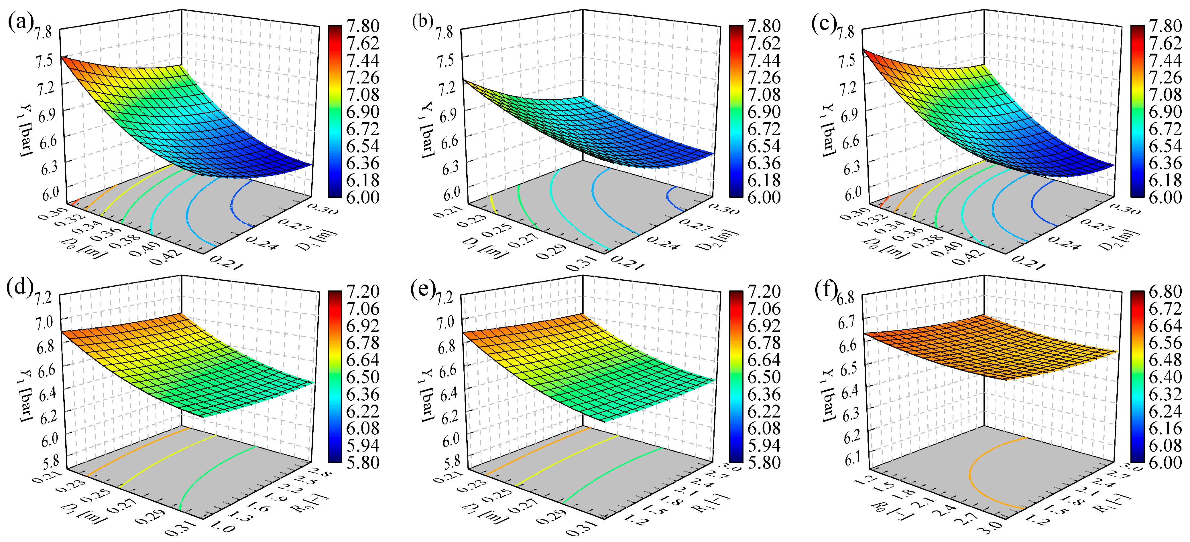
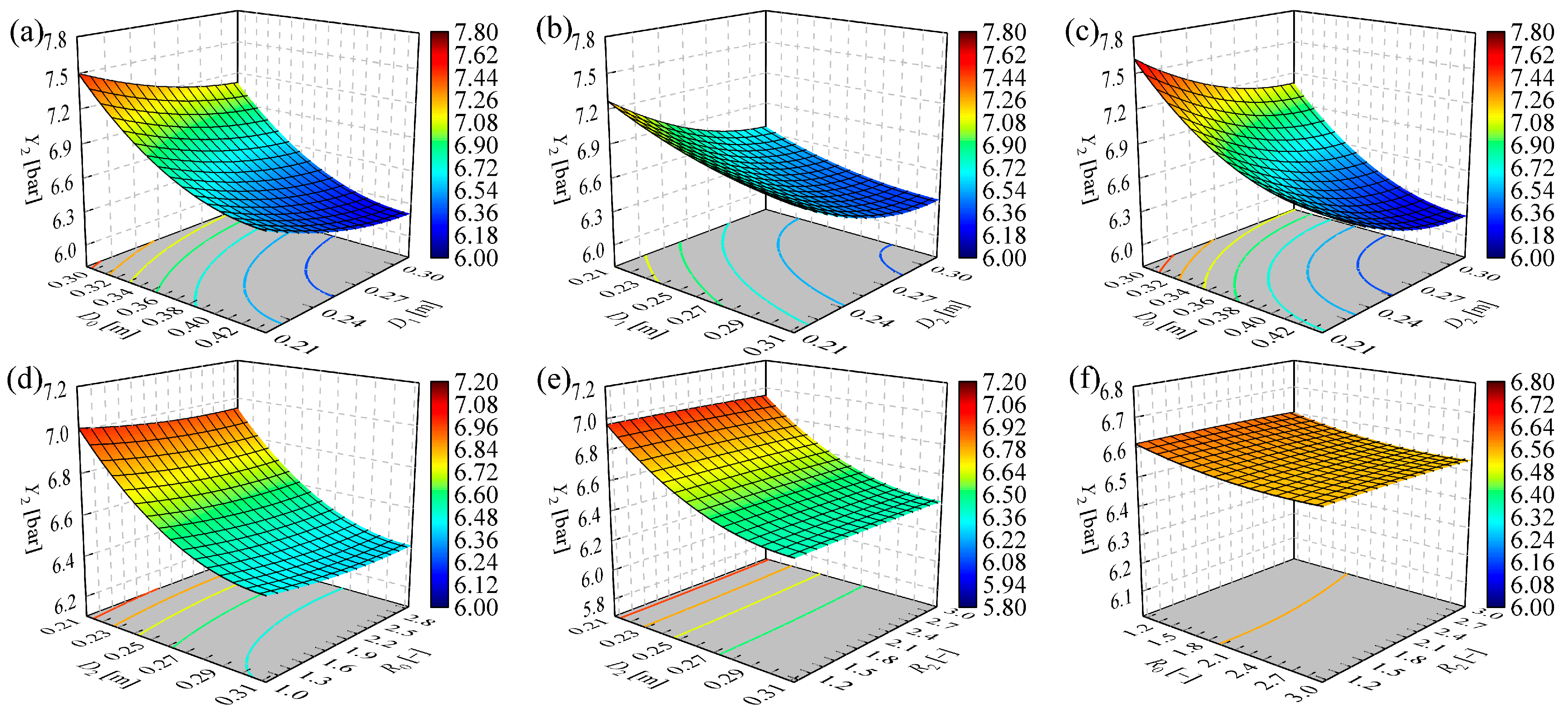
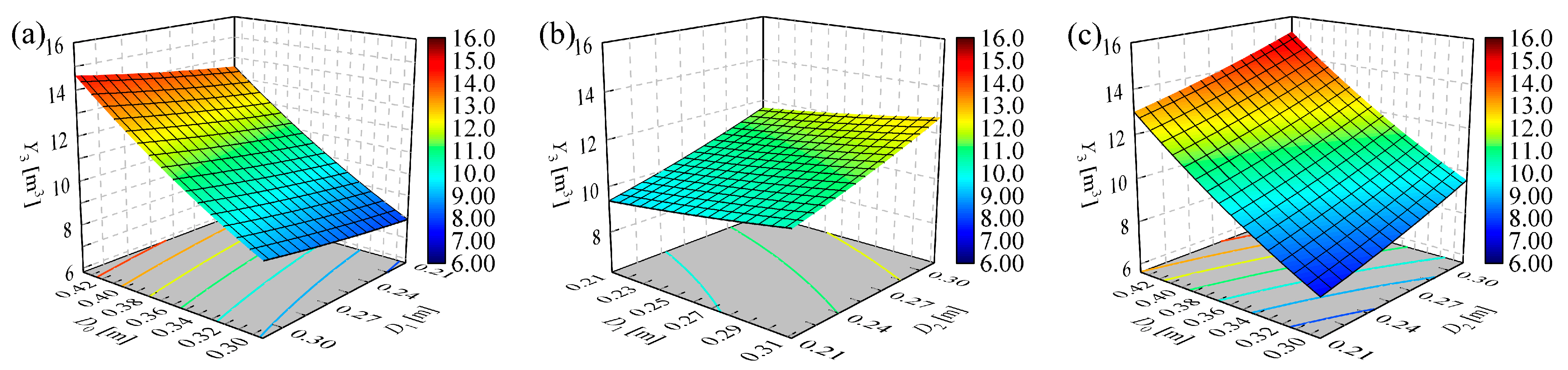
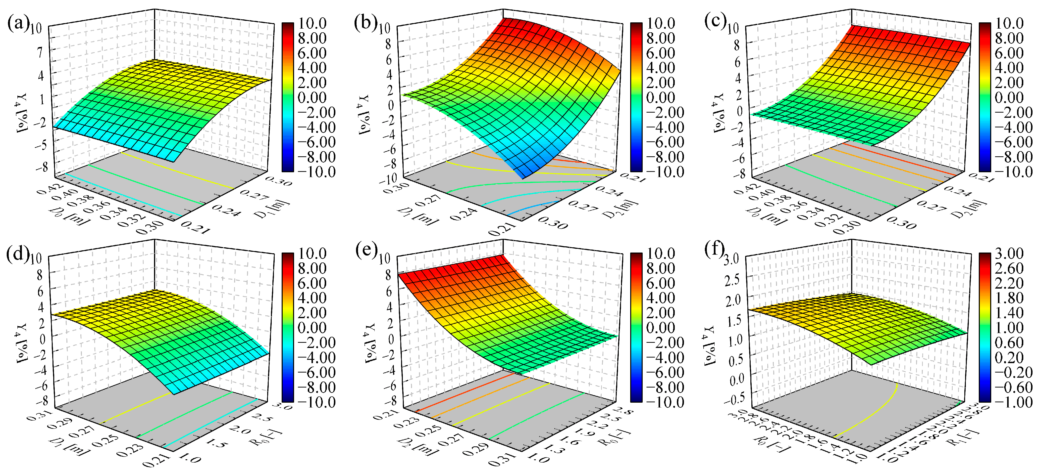
4.1. Response Surface Parameter Analysis

Based on the regression equation, the response surfaces of Y1, Y2, Y3, and Y4 were established and are shown in Figure 8, Figure 9, Figure 10 and Figure 11. It can be observed that the effect of the pipeline diameter on Y1, Y2, Y3, and Y4 was greater than that of the bend ratio at any condition. It can be noted from Figure 8 and Figure 9 that the resistance of each branch (Y1, Y2) gradually decreased as the main pipeline diameter (D0) increased. This was because in a steady-flow pipeline system, increasing the total flow area can reduce the average velocity. Based on Equation (8), the resistance decreased sharply with the reduction in the fluid velocity and the increase in the pipe diameter. The effect of the change in the branch pipe diameter on Y1, Y2, Y3, and Y4 was same as that of the main pipeline diameter. Similarly, for the pipe bend, increasing the bend–diameter ratio (R/D) could reduce the resistance of each branch, as expected. This was due to the increase in R/D reducing the local resistance coefficient. In addition, a bend with larger R/D can reduce turbulent losses, making the fluid more uniform in the bend and reducing the local loss.
Based on the above analysis, it was found that increasing the pipe diameter and the bend–diameter ratio (R/D) could reduce the resistance of the system. However, according to the volume calculation, as per Equation (1), increasing either the pipe diameter or R/D could increase the weight of the pipeline due to the pipeline system volume (Y3) increasing. This will decrease the fuel storage capacity of the replenishment oiler, thereby reducing its endurance during the supplying process. As can be seen from Figure 10, the pipeline diameter had a greater influence on Y3. This was due to the fact that the #0 pipeline had a large diameter and long length in the whole pipeline system, and it had a greater contribution to the overall pipeline volume. As we know, the pipeline system volume increases with the increase in R/D, but due to the low number of bends and their smaller size compared to the pipes, their contribution to the pipeline system volume was not important.
Figure 11 demonstrates the effect of pipeline selection on the flow imbalance (Y4). From the figure, it can be seen that the main pipeline diameter (D0) had a minor influence on Y4. In the steady-flow system, the diversion was not affected by D0, so D0 had little contribution to Y4. The resistance of branch #1 decreased with the increase in the pipe diameter of branch #1 (D1), resulting in more fluid being diverted from the main line to branch #1. Therefore, the flow imbalance between the two refueling stations increased. However, the opposite conclusion was obtained for branch #2. These results were achieved because the length of branch #2 was longer than branch #1 in the initial design of the pipeline system, resulting in a larger resistance. Hence, the branch #2 had a smaller volume flow rate caused by a weak separation effect compared to branch #1. As the diameter of branch #2 (D2) increased, the resistance gap between the two branches decreased. As a result, the flow in the two branches gradually became balanced. As revealed in Figure 11, the contribution of R/D to the flow imbalance was not obvious. This was because R/D had little effect on the resistance, and it therefore had no impact on the flow separation. Based on the above analysis, the original design scheme had a high optimization space, and the system optimization is described in Section 4.2.

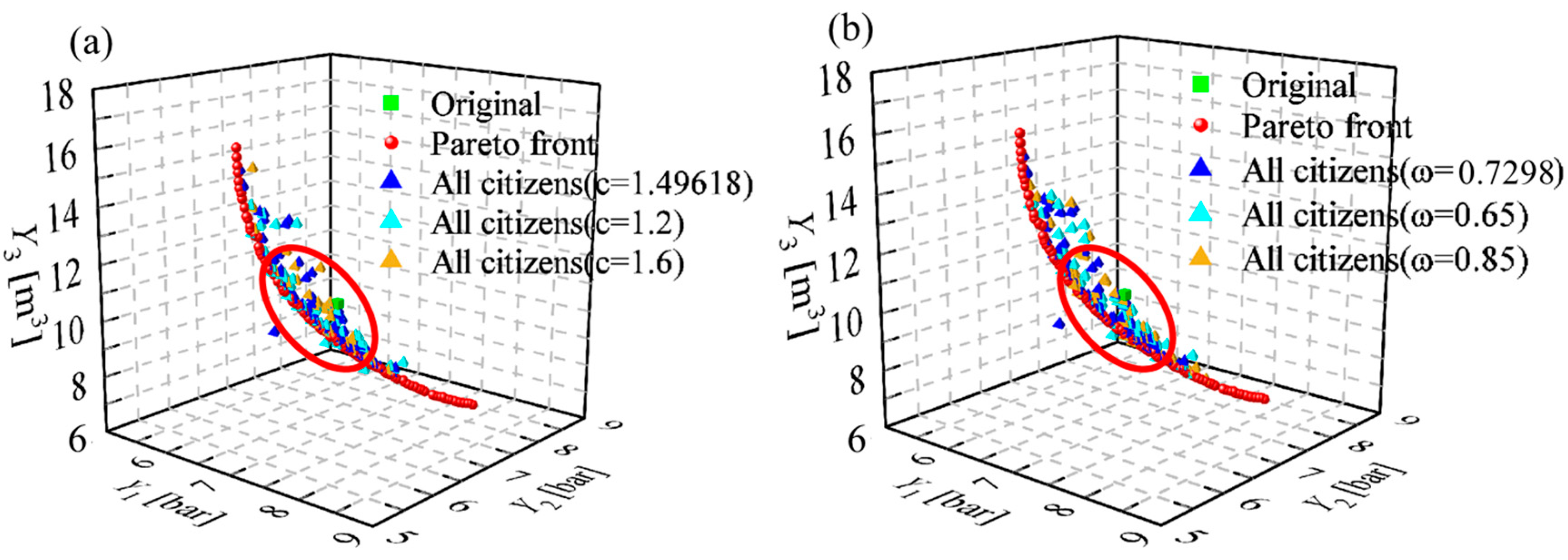
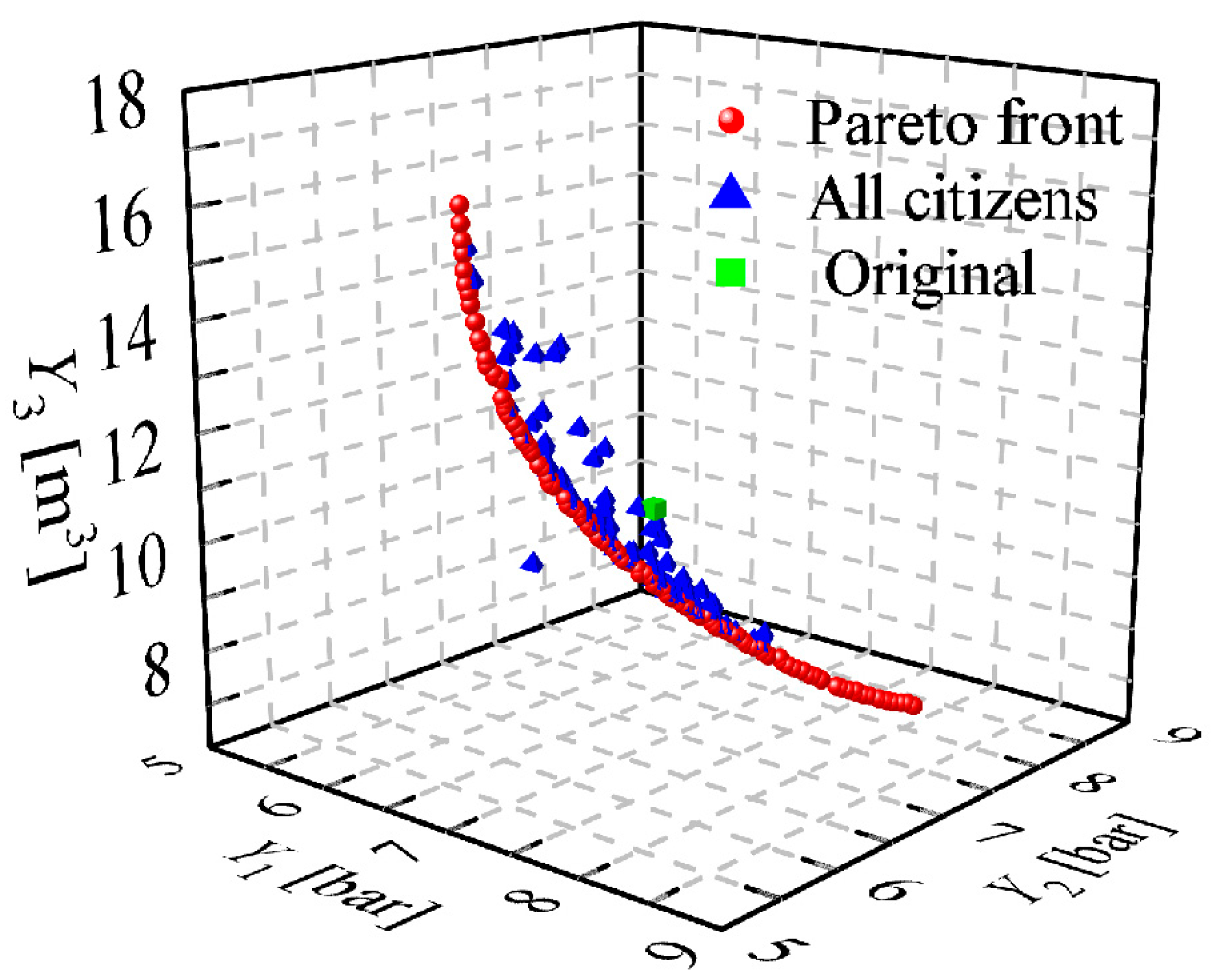
4.2. Multi-Objective Parameter Optimization with MOPSO

The aim of this study is to obtain the optimal selection scheme for the pipeline system. Therefore, an intelligent optimization algorithm was employed in this study in order to reduce the resistance and the volume of the pipeline system. According to the optimization process illustrated in Figure 2, the RSM regression model was used as an alternative model, and it was then combined with the MOPSO algorithm for optimization. The spatial distribution of Y1, Y2, and Y3 for all solutions after optimization is shown in Figure 12. The red dots in the figure are the optimal Pareto fronts, which represent the best solutions. The blue tetrahedra are all citizens, indicating all possible solutions, and the green square is the original design solution.
In this study, we expected to obtain the pipeline selection scheme that minimizes the resistance as well as the space volume of the pipeline system while ensuring the flow balance, as shown in Equation (2). According to the optimization results of MOPSO, a merit selection based on the “Practical Handbook of Ship Design-Engine Section” [18] needed to be performed. First, the schemes with a flow imbalance greater than 5% (i.e., Y4 > 5%) were filtered out from all the options. Second, the solutions with a pipeline system volume larger than 10 m3 (i.e., Y3 > 10 m3) were excluded (Y3 = 10.209 m3 for the original scheme). Finally, the solutions with a resistance higher than 6.89 bar (i.e., Y1 > 6.89 bar) for branch #1 and #2 (i.e., Y2 > 6.89 bar) were screened out (Y1 = 6.897 bar, Y2 = 6.891 bar for the original design scheme). The optimal filtered design solutions and their calculation results are shown in Table 2. According to the design requirements of the replenishment oiler, it was necessary to select the pipeline selection scheme that minimized the resistance of the pipeline; therefore, Case 1 was considered to be the optimal solution.
The optimization relied on mathematical models that may not fully align with existing national design standards, highlighting a gap between theoretical and practical applications; thus, it was necessary to standardize the selection according to the “Practical Handbook of Ship Design-Engine Section” [18]. The corresponding parameters in Case 1 were determined as D0 = DN340, D1 = DN280, D2 = DN260, R0 = 1.5, R1 = 1.5, and R2 = 1. Before optimization, the parameters were D0 = DN300, D1 = DN300, D2 = DN300, R0 = 3, R1 = 3, and R2 = 3. Both the original design and the optimized Case 1 were simulated by the Flowmaster software simultaneously, and the results are shown in Figure 13. It can be seen that the RSM-MOPSO-optimized Case 1 significantly reduced the resistance of each branch and the pipeline system volume. Compared with the original design, the RSM-MOPSO-optimized Case 1 reduced the resistance of branches #1 (Y1) and #2 (Y2) by 3.57% and 3.51%. The overall pipeline system volume (Y3) was reduced by 5.72%. The flow imbalance (Y4) of Case 1 was 1.59%, which satisfies the design requirements within 5%.

5. Conclusions

In this paper, the optimization of pipeline selection for a replenishment oiler pipeline system was carried out based on the RSM-MOPSO method. The main conclusions of this study are as follows:
(1)
A 1D Flowmaster simulation model was developed based on the replenishment oiler pipeline system and was validated by completed ship data. Good agreement was obtained, confirming the accuracy of the simulation model, and the maximum error of the model was 4.44%, which is below the allowable error in engineering of 5%.
(2)
The RSM method was employed to establish regression prediction models for the resistance of the deck refueling pipelines #1 (Y1) and #2 (Y2), the pipeline system volume (Y3), and the flow imbalance between the two supply ports (Y4). The analysis of variance (ANOVA) result was greater than 0.98, proving the strong predictability of the regression models.
(3)
The regression equation established by RSM was combined with the intelligent optimization algorithm MOPSO to optimize the pipeline selection.
(4)
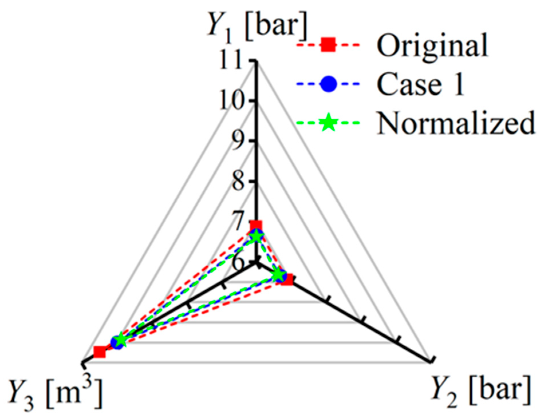
Due to the optimization results only considering mathematical relationships, they did not satisfy the national standards and needed to be standardized according to the “Practical Handbook of Ship Design-Engine Section”. The processed results show that the resistance of the deck refueling pipeline #1 (Y1) and #2 (Y2) were reduced by 3.57% and 3.51%, respectively. The pipeline system volume (Y3) was reduced by 5.72%. The simulation results indicate that optimized pipeline selection in replenishment oilers can achieve the dual objectives of resistance reduction and spatial efficiency improvement, thus significantly enhancing in-service refueling performance.
In conclusion, this study presents a method for pipeline system selection in replenishment oilers by integrating machine learning with optimization algorithms. The proposed approach enables the rapid generation of pipeline design solutions, thereby shortening development timelines, minimizing design revisions, and, ultimately, enhancing the overall efficiency of pipeline system design for maritime replenishment operations. Moreover, the achievement of this study demonstrates that pipeline selection optimization can still enhance the performance of the pipeline system even after finalizing the pipeline route design. By incorporating pipeline selection optimization into the design process, replenishment oilers could achieve significant improvements in operational efficiency and refueling performance.
In future work, we will consider the influence of the actual cabin structure and combine pipe parameter selection with pipe route planning for a more systematic pipeline system design.

Author Contributions

Conceptualization, Y.C. and C.M.; methodology, Y.C. and C.M.; software, M.Y. and Y.L.; validation, Y.C., P.Y., and T.L.; formal analysis, P.Y.; investigation, M.Y.; resources, C.M. and T.L.; data curation, S.H.; writing—original draft preparation, Y.C.; writing—review and editing, P.Y.; visualization, Y.C.; supervision, Y.L.; project administration, T.L.; funding acquisition, P.Y. All authors have read and agreed to the published version of the manuscript.

Funding

This research was funded by the National Natural Science Foundation of China (52371330) and Ocean Defense Innovation Fund (2022).

Institutional Review Board Statement

Not applicable.

Informed Consent Statement

Not applicable.

Data Availability Statement

The original contributions presented in this study are included in the article. Further inquiries can be directed to the corresponding author.

Acknowledgments

The authors also gratefully acknowledge the helpful comments and suggestions of the reviewers, which have improved the presentation of this paper.

Conflicts of Interest

The authors declare no conflicts of interest.

Abbreviations

The following abbreviations are used in this manuscript:
SPDShip pipeline design
RSMResponse surface methodology
ANOVAAnalysis of variance
MOPSOMulti-objective particle swarm optimization
R/DBend–diameter ratio
PSOParticle swarm optimization

Appendix A

To demonstrate the robustness of the proposed optimization framework, we conducted a configuration analysis based on another pipeline system, and the Flowmaster model is shown as Figure A1, which exhibits a layout entirely distinct from the pipeline system in the baseline study. Utilizing the same methodology outlined in the original work, we first constructed an RSM surrogate model and subsequently solved the problem via the MOPSO algorithm. The resulting Pareto solution distributions are illustrated in Figure A2a (new system) and Figure A2b (system in the original manuscript). The results show that regardless of the changes in the system layout, this optimized methodology could consistently identify the optimal solution range. As highlighted by the red bounding boxes in Figure A2 (nearly 75% of the points are in the red box in both Figure A2a,b), the majority of optimal solutions clustered near predefined reference points (original design), demonstrating strong consistency in global optimization trends and validating the framework’s independence from specific system configurations.
Figure A1. One-dimensional simulation model for another pipeline system based on the Flowmaster software. P1–P22 are pipes, B1–B10 are bends, J1–J4 are junctions, V1–V6 are butterfly valves, Fi1 is a filter, Fm1 is a flowmeter, F is the flow boundary, P is the pressure boundary, S1–S2 are supply ports, and E1–E3 are end boundaries.
Jmse 13 01037 g0a1
Figure A2. Comparison of overall distribution of goals between two system layouts: (a) new system; (b) original system.
Jmse 13 01037 g0a2
In this study, we conducted a sensitivity analysis of the weight factor (0.4 < ω < 0.9) and the learning factor (1 < c <2), as displayed in Figure A3a,b, respectively. From Figure A3, it can be seen that different learning factors and weight factors had little effects on the distribution of the MOPSO results, and most of the solution sets were distributed near the original design point (about 70% of the points fall within the red ellipse), which indicates that the results of this study are independent of the learning factors and weight factors, and the use of a learning factor of 1.49618 and a weighting factor of 0.7298 was reasonable. In addition, Figure A3 also shows that almost all the solutions were distributed near the Pareto front, which indicates that the algorithm has good convergence and searchability and does not fall into the dilemma of local optimality.
Figure A3. Optimal solution sets with different parameters: (a) learning factor; (b) weight factor.
Jmse 13 01037 g0a3

References

  1. Fagerholt, K.; Hvattum, L.M.; Johnsen, T.A.V.; Korsvik, J.E. Routing and scheduling in project shipping. Ann. Oper. Res. 2013, 207, 67–81. [Google Scholar] [CrossRef]
  2. Iris, Ç.; Lam, J.S.L. A review of energy efficiency in ports: Operational strategies, technologies and energy management systems. Renew. Sustain. Energy Rev. 2019, 112, 170–182. [Google Scholar] [CrossRef]
  3. Christiansen, M.; Fagerholt, K.; Nygreen, B.; Ronen, D. Ship routing and scheduling in the new millennium. Eur. J. Oper. Res. 2013, 228, 467–483. [Google Scholar] [CrossRef]
  4. Yan, W.; Yang, M.; Lin, Y. A hybrid algorithm based on the proposed square strategy and NSGA-II for ship pipe route design. Ocean Eng. 2024, 305, 117961. [Google Scholar] [CrossRef]
  5. Guarracino, F.; Fraldi, M.; Giordano, A. Analysis of testing methods of pipelines for limit state design. Appl. Ocean Res. 2008, 30, 297–304. [Google Scholar] [CrossRef]
  6. Kyrkjebø, E.; Pettersen, K.Y.; Wondergem, M.; Nijmeijer, H. Output synchronization control of ship replenishment operations: Theory and experiments. Control Eng. Pr. 2007, 15, 741–755. [Google Scholar] [CrossRef]
  7. Dong, Z.; Luo, W. Ship pipe route design based on NSGA-III and multi-population parallel evolution. Ocean Eng. 2024, 293, 116666. [Google Scholar] [CrossRef]
  8. Huang, H.; Yuan, Z.; Qian, H.; Ye, Y.; Leng, J.; Wei, Y. Design and analysis of a novel ship pipeline welding auxiliary device. Ocean Eng. 2016, 123, 55–64. [Google Scholar] [CrossRef]
  9. Wang, Y.; Zhang, Y.; Wang, W.; Liu, Z.; Yu, X.; Li, H.; Wang, W.; Hu, X. A review of optimal design for large-scale micro-irrigation pipe network systems. Agronomy 2023, 13, 2966. [Google Scholar] [CrossRef]
  10. Yeo, I.; Roh, M.; Chun, D.; Jang, S.H.; Heo, J.W. Optimal arrangement design of pipeline support by considering safety and production cost. Int. J. Nav. Archit. Ocean. Eng. 2023, 15, 100531. [Google Scholar] [CrossRef]
  11. Blokland, M.; Van der Mei, R.D.; Pruyn, J.F.J.; Berkhout, J. Literature survey on automatic pipe routing. Oper. Res. Forum 2023, 4, 35. [Google Scholar] [CrossRef]
  12. Park, J.; Storch, R.L. Pipe-routing algorithm development: Case study of a ship engine room design. Expert Syst. Applications 2002, 23, 299–309. [Google Scholar] [CrossRef]
  13. Zhang, H.; Yu, Y.; Zhang, Q.; Yang, Y.; Liu, H.; Lin, Y. A bidirectional collaborative method based on an improved artificial fish swarm algorithm for ship pipe and equipment layout design. Ocean Eng. 2024, 296, 117045. [Google Scholar] [CrossRef]
  14. Lin, Y.; Zhang, Q. A multi-objective cooperative particle swarm optimization based on hybrid dimensions for ship pipe route design. Ocean Eng. 2023, 280, 114772. [Google Scholar] [CrossRef]
  15. Ha, J.; Roh, M.; Kim, K.; Kim, J. Method for pipe routing using the expert system and the heuristic pathfinding algorithm in shipbuilding. Int. J. Nav. Arch. Ocean 2023, 15, 100533. [Google Scholar] [CrossRef]
  16. Wang, Y.; Yu, Y.; Li, K.; Zhao, X.; Guan, G. A human-computer cooperation improved ant colony optimization for ship pipe route design. Ocean Eng. 2018, 150, 12–20. [Google Scholar] [CrossRef]
  17. Min, J.; Ruy, W.; Park, C.S. Faster pipe auto-routing using improved jump point search. Int. J. Nav. Arch. Ocean 2020, 12, 596–604. [Google Scholar] [CrossRef]
  18. Huang, H. Practical Handbook of Ship Design-Engine Section, 3rd ed.; National Defense Industry Press: Beijing, China, 2013. [Google Scholar]
  19. Rai, P.K.; Kant, V.; Sharma, R.K.; Gupta, A. Process optimization for textile industry-based wastewater treatment via ultrasonic-assisted electrochemical processing. Eng. Appl. Artif. Intell. 2023, 122, 106162. [Google Scholar] [CrossRef]
  20. Li, J.; Jasim, D.J.; Kadir, D.H.; Maleki, H.; Esfahani, N.N.; Shamsborhan, M.; Toghraie, D. Multi-objective optimization of a laterally perforated-finned heat sink with computational fluid dynamics method and statistical modeling using response surface methodology. Eng. Appl. Artif. Intell. 2024, 130, 107674. [Google Scholar] [CrossRef]
  21. Coppedè, A.; Gaggero, S.; Vernengo, G.; Villa, D. Hydrodynamic shape optimization by high fidelity CFD solver and Gaussian process based response surface method. Appl. Ocean Res. 2019, 90, 101841. [Google Scholar] [CrossRef]
  22. Cao, Y.; Khan, A.; Abdi, A.; Ghadiri, M. Combination of RSM and NSGA-II algorithm for optimization and prediction of thermal conductivity and viscosity of bioglycol/water mixture containing SiO2 nanoparticles. Arab. J. Chem. 2021, 14, 103204. [Google Scholar] [CrossRef]
  23. Zhang, Z.; Dong, R.; Tan, D.; Zhang, B. Multi-objective optimization of performance characteristic of diesel particulate filter for a diesel engine by RSM-MOPSO during soot loading. Process Saf. Environ. Prot. 2023, 177, 530–545. [Google Scholar] [CrossRef]
  24. Li, R.; Gao, Y.; Jiang, B.; Lv, M.; Li, H. Intelligent parameter optimization of sealed airbag vessels with preventing water hammer in cascaded pressurized water transmission system: Based on MOPSO algorithm. J. Water Process Eng. 2025, 70, 106915. [Google Scholar] [CrossRef]
  25. Wang, Y.; Iris, Ç. Transition to near-zero emission shipping fleet powered by alternative fuels under uncertainty. Transp. Res. Part. D. Transp. Environ. 2025, 142, 104689. [Google Scholar] [CrossRef]
  26. Gu, Y.; Wang, Y.; Iris, Ç. Integrated Green Technology adoption, ship speed optimization and slot management for shipping alliance under emission limits and uncertain fuel prices. J. Clean. Prod. 2025, 494, 144939. [Google Scholar] [CrossRef]
  27. Bouchaala, A.; Merroun, O.; Sakim, A. A MOPSO algorithm based on pareto dominance concept for comprehensive analysis of a conventional adsorption desiccant cooling system. J. Build. Eng. 2022, 60, 105189. [Google Scholar] [CrossRef]
  28. Liu, J.; Zhao, H.; Wang, J.; Zhang, N. Optimization of the injection parameters of a diesel/natural gas dual fuel engine with multi-objective evolutionary algorithms. Appl. Therm. Eng. 2019, 150, 70–79. [Google Scholar] [CrossRef]
  29. Yin, L.; Ding, W. Multi-objective high-dimensional multi-fractional-order optimization algorithm for multi-objective high-dimensional multi-fractional-order optimization controller parameters of doubly-fed induction generator-based wind turbines. Eng. Appl. Artif. Intell. 2023, 126, 106929. [Google Scholar] [CrossRef]
  30. Shuai, W.; Xiaohui, L.; Xiaomin, H. Multi-objective optimization of reservoir flood dispatch based on MOPSO algorithm. In Proceedings of the 8th International Conference on Natural Computation, IEEE, Chongqing, China, 29–31 May 2012. [Google Scholar]
  31. Kennedy, J.; Eberhart, R. Particle swarm optimization. In Proceedings of the ICNN’95—International Conference on Neural Networks, Perth, Australia, 27 November–1 December 1995. [Google Scholar]
  32. Coello Coello, C.A.; Lechuga, M.S. MOPSO: A proposal for multiple objective particle swarm optimization. In Proceedings of the 2002 Congress on Evolutionary Computation (Cat. No.02TH8600), Honolulu, HI, USA, 12–17 May 2002. [Google Scholar]
  33. Coello, C.A.C.; Pulido, G.T.; Lechuga, M.S. Handling multiple objectives with particle swarm optimization. IEEE Trans. Evol. Comput. Publ. Information. 2004, 8, 256–279. [Google Scholar] [CrossRef]
  34. Pang, L.; Ng, S.; Aguirre, H. Improved efficiency of MOPSO with adaptive inertia weight and dynamic search space. In Proceedings of the Genetic and Evolutionary Computation Conference Companion, Kyoto, Japan, 15–19 July 2018. [Google Scholar]
  35. Zhang, X.; Liu, H.; Tu, L. A modified particle swarm optimization for multimodal multi-objective optimization. Eng. Appl. Artif. Intell. 2020, 95, 103905. [Google Scholar] [CrossRef]
  36. Ali, T.; Peng, Y.; Jin, Z.H.; Kun, L.; Renchuan, Y. Crashworthiness optimization method for sandwich plate structure under impact loading. Ocean Eng. 2022, 250, 110870. [Google Scholar] [CrossRef]
  37. Tuppadung, Y.; Kurutach, W. Comparing nonlinear inertia weights and constriction factors in particle swarm optimization. Int. J. Knowl.-Based Dev. 2011, 15, 65–70. [Google Scholar] [CrossRef]
  38. Vandenbergh, F.; Engelbrecht, A. A study of particle swarm optimization particle trajectories. Inf. Sci. 2006, 176, 937–971. [Google Scholar] [CrossRef]
  39. Eberhart, R.C.; Shi, Y. Comparing inertia weights and constriction factors in particle swarm optimization. In Proceedings of the 2000 Congress on Evolutionary Computation, La Jolla, CA, USA, 16–19 July 2000. [Google Scholar]
  40. Cong, Y.; Gan, H.; Wang, H.; Hu, G.; Liu, Y. Multi-objective optimization of the performance and emissions of a large low-speed dual-fuel marine engine based on MNLR-MOPSO. J. Mar. Sci. Eng. 2021, 9, 1170. [Google Scholar] [CrossRef]
  41. Huang, Y.; Ma, F. Intelligent regression algorithm study based on performance and NOx emission experimental data of a hydrogen enriched natural gas engine. Int. J. Hydrogen Energy. 2016, 41, 11308–11320. [Google Scholar] [CrossRef]
  42. Wang, H.; Ji, C.; Shi, C.; Ge, Y.; Wang, S.; Yang, J. Development of cyclic variation prediction model of the gasoline and n-butanol rotary engines with hydrogen enrichment. Fuel 2021, 299, 120891. [Google Scholar] [CrossRef]
  43. Kakati, D.; Roy, S.; Banerjee, R. Development of an artificial neural network based virtual sensing platform for the simultaneous prediction of emission-performance-stability parameters of a diesel engine operating in dual fuel mode with port injected methanol. Energy Convers. Management 2019, 184, 488–509. [Google Scholar] [CrossRef]
Figure 1. Schematic diagram of external refueling pipeline system for replenishment oiler.
Jmse 13 01037 g001
Figure 2. Flow chart of multi-objective optimization calculation.
Jmse 13 01037 g002
Figure 3. One-dimensional simulation model of the pipeline system based on the Flowmaster software. P1–P31 are pipes, B1–B15 are bends, J1–J6 are junctions, V1–V10 are butterfly valves, Fi1–Fi2 are filters, Fm1–Fm2 are flowmeters, F is the flow boundary, P is the pressure boundary, S1–S2 are supply ports, and E1–E3 are end boundaries.
Jmse 13 01037 g003
Figure 4. Schematic diagram of an A-type replenishment oiler for external refueling, where #d-1 is the supply port, Fi1–Fi2 are filters, and ①–⑤ are pumps.
Jmse 13 01037 g004
Figure 5. Validation of simulation model (The experimental data are from reference [18]).
Jmse 13 01037 g005
Figure 6. Comparison between the simulation and experimental results; the experimental data as well as the simulation data were normalized according to the shipyard’s confidentiality agreement.
Jmse 13 01037 g006
Figure 7. Comparison of prediction and simulation results: (ad) the comparison of the predicted and simulated values; (eh) the regression curve of Y1, Y2, Y3, and Y4.
Jmse 13 01037 g007aJmse 13 01037 g007b
Figure 8. Response surface plot of the #1 pipeline resistance (Y1): (af) the effect of D0 and D1, D1 and D2, D0 and D2, D1 and R0, D1 and R1, and R0 and R1 on Y1.
Jmse 13 01037 g008
Figure 9. Response surface plot of the #2 pipeline resistance (Y2): (af) the effect of D0 and D1, D1 and D2, D0 and D2, D2 and R0, D2 and R2, and R0 and R2 on Y2.
Jmse 13 01037 g009
Figure 10. Response surface plot of the pipeline system volume (Y3): (af) the effect of D0 and D1, D1 and D2, D0 and D2, D1 and R0, D2 and R0, and R0 and R1 on Y3.
Jmse 13 01037 g010aJmse 13 01037 g010b
Figure 11. Response surface plot of the flow imbalance (Y4): (af) the effect of D0 and D1, D1 and D2, D0 and D2, D1 and R0, D2 and R0, and R0 and R1 on Y4.
Jmse 13 01037 g011
Figure 12. Overall distribution of goals.
Jmse 13 01037 g012
Figure 13. Comparison of target variables before and after optimization.
Jmse 13 01037 g013
Table 1. ANOVA table for Y1, Y2, Y3, and Y4.
ItemY1Y2Y3Y4
F Valuep ValueF Valuep ValueF Valuep ValueF Valuep Value
Model1156.07<0.00011136.88<0.000121,195.29<0.00011356.51<0.0001
D118,551.16<0.000118,022.45<0.00014.67 × 105<0.00012.60.1188
D24016.35<0.00013511.88<0.000116,607.33<0.00019679.11<0.0001
D35828.64<0.00016387.27<0.000173,930.77<0.000121,070.05<0.0001
R192.95<0.000190.24<0.00018737.17<0.00010.04280.8377
R225.37<0.000121.83<0.00011114.75<0.000184.6<0.0001
R31.940.1752.190.1511123.84<0.000110.640.0031
D1D20.00020.99030.00010.99043.66 × 10−60.998501
D1D31.80.19171.960.17351.94 × 10−60.99895.930.022
D1R134.79<0.000133.78<0.00011801.85<0.00010.06420.802
D1R21.21 × 10−60.99911.18 × 10−60.99911.21 × 10−70.99970.12840.723
D1R33.10 × 10−60.99863.81 × 10−60.99851.21 × 10−70.999700.9974
D2D337.46<0.000139.06<0.00013.03 × 10−80.999945.74<0.0001
D2R101013.03 × 10−80.999901
D2R210.710.0039.230.0054229.21<0.000133.1<0.0001
D2R30.09950.7550.08620.77143.02 × 10−60.99860.27310.6057
D3R14.85 × 10−80.99984.70 × 10−80.99982.45 × 10−60.998801
D3R20.04240.83840.04080.84161.48 × 10−60.9990.00190.9656
D3R30.8040.37810.87860.357225.46<0.00012.840.1041
R1R24.85 × 10−80.99984.70 × 10−80.9998010.12840.723
R1R34.85 × 10−80.99984.70 × 10−80.99983.03 × 10−80.999901
R2R30.08180.77720.07020.79313.02 × 10−60.99860.26610.6103
D121945.43<0.00011884.7<0.00012565.48<0.00012.270.144
D22275.06<0.0001230.42<0.0001113.08<0.00011277.35<0.0001
D32629.78<0.0001690.12<0.0001334.91<0.00012281.39<0.0001
R1219.330.000219.150.00026.93 × 10−70.99931.570.2207
R229.530.00488.590.0074.61 × 10−70.999513.310.0012
R320.49710.4870.52120.47682.42 × 10−60.99880.63420.433
R 2 0.99920.999210.9993
R A d j . 2 0.99830.99830.99990.9986
R Pr e d . 2 0.99570.99560.99980.9963
Table 2. Optimal solutions for satisfying constraints.
CaseD0 [m]D1 [m]D2 [m]R0 [−]R1 [−]R2 [−]Y1 [bar]Y2 [bar]Y3 [bar]Y4 [%]
10.3420.2840.2561.6061.4341.1646.6686.6789.9822.728
20.3450.2870.2541.0951.6101.0176.6846.6969.8973.009
30.3420.2860.2461.3881.3041.1036.7396.7539.6713.568
40.3460.2840.2439241.0001.1071.6996.7666.7799.5853.750
50.3450.2720.2451.2461.2731.3386.7856.7979.5343.239
60.3440.2740.2441.1811.3721.0006.7916.8049.4883.479
70.3390.2760.2461.2891.1931.0156.8086.8209.4033.231
80.3260.2840.2551.6691.0841.0576.8356.8459.3162.614
90.3420.2760.2391.0781.0001.0006.8556.8709.2523.987
Disclaimer/Publisher’s Note: The statements, opinions and data contained in all publications are solely those of the individual author(s) and contributor(s) and not of MDPI and/or the editor(s). MDPI and/or the editor(s) disclaim responsibility for any injury to people or property resulting from any ideas, methods, instructions or products referred to in the content.

