An Experimental Study on the Effects of Deflector Baffles and Circular Fish School Swimming Patterns on Flow Field Characteristics in Aquaculture Vessels

Abstract

To maximize the limited space of aquaculture vessels and achieve a more efficient layout for aquaculture compartments at the bow and stern, this study proposes two design schemes: modifying the compartment configuration and removing the deflector baffle. The study focused on the impact of compartment configuration and fish movement on the flow field characteristics under the two proposed schemes. The results showed that the mean flow velocity in the octagonal tanks was higher at jet angles of 30° and 45°, with the trend index ($\gamma$) being more stable at 30°. Within jet angles ranging from 0° to 45°, the mean flow velocity increased with rising jet velocity. Retaining the deflector baffle helped stabilize the flow field, making it more effective than scheme A, which, in turn, outperformed scheme B. In circular tanks, the mean flow velocity was higher at 0° and 15°, with the trend index being more stable at 0°. Retaining the deflector baffle at low jet angles further stabilized the flow field. Retaining the deflector baffle at low jet angles helped maintain high average flow velocity, while at high jet angles, it reduced turbulence. Therefore, scheme A demonstrated a better balance between aquaculture volume and flow field stability. Fish simulation experiments revealed that the presence of fish significantly hinders fluid flow and disrupts the stability of the flow field. In practical aquaculture, the jet angle and the use of deflector baffles should be selected based on the tank geometry, while the jet velocity should be adjusted according to the fish species and their swimming speed to establish a flow environment conducive to fish survival and growth.

1. Introduction

With the global population increasing and the demand for high-quality protein rising, the sustainable utilization of marine fishery resources has become a critical concern. In recent years, deep-sea aquaculture vessels have emerged as an innovative mode of marine fishery production, attracting increasing attention due to their high efficiency, environmental protection and sustainability [1]. By extending aquaculture zones from coastal areas to the deep sea, aquaculture vessels capitalize on the superior water quality and natural environmental conditions of the open ocean, offering fish a broader and healthier growth environment [2]. Moreover, during the aquaculture process, a suitable water environment can be created by precisely controlling the flow rate in accordance with the growth habits of the fish, thereby promoting better development. Additionally, the aquaculture vessel can be designed to optimize spatial utilization based on its structural characteristics, thereby increasing aquaculture capacity and effectively improving yield.

In aquaculture tank flow field studies, the deflector baffle is a key structural component, and its appropriate configuration can significantly influence the direction and velocity distribution of the flow field. Masaló et al. compared the flow field distribution in a rectangular tank with baffles and showed that placing a baffle between the two inlets enhances the fluid velocity and uniformity in the tank [3]. Gorle et al. investigated the flow velocity, flow uniformity, and vortex characteristics in an octagonal cell using the CFD method and found that the vortex columns disappeared and the rotational velocity was significantly reduced in an octagonal cell in the limit case of pure wall drainage [4]. Davidson et al. conducted physical experiments to examine the relationship between fluid dynamics and solid particle transport in circular tanks, concluding that optimizing the central rotational velocity facilitates the settling and discharge of solids [5].

The movement of fish can affect the distribution of the flow field in an aquaculture tank, which is a complex hydrodynamic problem. There is a direct relationship between the flow velocity of the artificial flow field and the body length of the aquacultured fish, and aquaculture studies have shown that the flow velocity of the artificial flow field is optimal for fish swimming when it is 1.5 to 2 times the body length of the fish [5]. Uniform flow velocity in the flow field with fewer eddy and turbulent areas is beneficial for fish swimming [6]. Compared to fish in marine environments, fish in tank-based systems exhibit more predictable movement trajectories, and their presence significantly reduces both mean flow velocity and flow field uniformity. The artificial flow field inside aquaculture tanks is related to the species of cultured fish and their swimming behaviors; turbulence induced by fish movement further impacts the distribution of dissolved oxygen, metabolic waste, feces, and uneaten feed [7,8]. When investigating the flow field characteristics in aquaculture tanks, it is essential to account for the hydrodynamic impact of fish. Most existing studies simulate the hydrodynamic influence of a single fish’s tail-swinging motion; however, modeling the collective behavior of multiple fish requires constructing multi-fish models, significantly increasing computational complexity and resource demands. Some researchers employ moving-grid methods to model fish-induced flow disturbances, but this necessitates mesh refinement near fish bodies, increasing computational load, while excessive movement may cause numerical instability and result dispersion.

Unlike land-based tanks, the tank structure of an aquaculture vessel has top and bottom side compartments that act as shock absorbers, and the diameter-to-depth ratio of these tanks (1.1–2.5) [9,10] is much smaller than that of land-based tanks (4–8.17) [11,12]. There are fewer studies based on the characteristics of the water environment under the special structure of aquaculture tanks. For example, Xiong et al. [6] examined how the number of intake pipes and the bottom water discharge rate affect the removal rate of solid particles, including feces and residual feed, in aquaculture tanks. Their findings demonstrated that the bottom water discharge rate has a negligible impact on the discharge of solid particles. In another study, Xue et al. [13] explored the influence of aquaculture tank structures on the fluid properties and the solid particle removal rate. They found that rounding the two right-angled corners of rectangular tanks significantly improved the internal flow characteristics.

Within aquaculture vessel compartments, a complex interaction exists between fish swimming behavior and the surrounding flow field. On the one hand, a reasonable flow field design can provide a suitable water flow environment for the fish to promote their healthy growth [14,15]; On the other hand, fish swimming behavior exerts feedback on the flow field, changing the speed, direction and distribution of the water flow [16,17]. This interaction not only affects the growth and welfare of the fish population, but may also have a significant impact on the energy consumption of the aquaculture vessels and aquaculture efficiency. Some scholars have conducted studies using physical test methods such as rhodamine fluorescence and acoustic Doppler velocimetry, and have found that fish have a more pronounced effect on water homogeneity, that the intensity of turbulence is increased in tanks with fish, and that the presence of fish has a greater effect on flow field characteristics [18]. Masalo et al. [19] investigated the effect of fish swimming on the mean flow velocity and flow profiles in a circular pool and showed that turbulence caused by fish swimming increased the kinematic eddy viscosity, leading to a significant decrease in velocity near the center of the outlet flume. As the application of Computational Fluid Dynamics (CFD) technology in the optimization of tank parameters is becoming more and more mature, many scholars have carried out preliminary studies on the interactions between farmed fish and the characteristics of the tank’s flow field [20,21]. Liu Haibo et al. [22] used Sebastes schlegelii as a bionic object to establish a three-dimensional numerical model coupled with a cultured flow field, and simulated the effect of the shedding vortex formed by the tail swing of the fish on the flow field in the tank. The interaction between fish and the flow field will be affected by factors such as fish density, individual body size, spatial distribution, etc. Investigating how these factors affect flow field characteristics is essential for understanding the coupling mechanisms between fish swimming behavior and hydrodynamics in aquaculture systems. Although extensive research has been conducted globally on recirculating aquaculture system (RAS) flow field design [23,24], most studies have overlooked the influence of cultured fish on flow field dynamics. Most of the studies on the effects of fish on the flow field characteristics of aquaculture ponds are based on actual measurement methods, and there are fewer studies on the effects of farmed fish on the flow field characteristics of aquaculture ponds using experimental methods. While fish adjust their swimming direction, speed, and formation in response to flow field variations, the specific mechanisms of these adjustments on the flow field are not clear. Additionally, variations in the flow field can affect fish physiology and behavior, ultimately influencing their growth and health.

Therefore, a comprehensive investigation into the effects of deflector baffles and fish movement on the internal flow field of aquaculture vessels is crucial for optimizing vessel design and operation, enhancing farming efficiency and fish welfare, and advancing deep-sea aquaculture technologies. This study aims to systematically examine how deflector baffle configurations and fish movement patterns influence flow field dynamics within aquaculture vessels. Experimental methods are employed to reveal the underlying mechanisms and offer design optimization strategies, providing theoretical foundations and technical guidance for efficient vessel operation.

2. Experimental Methods

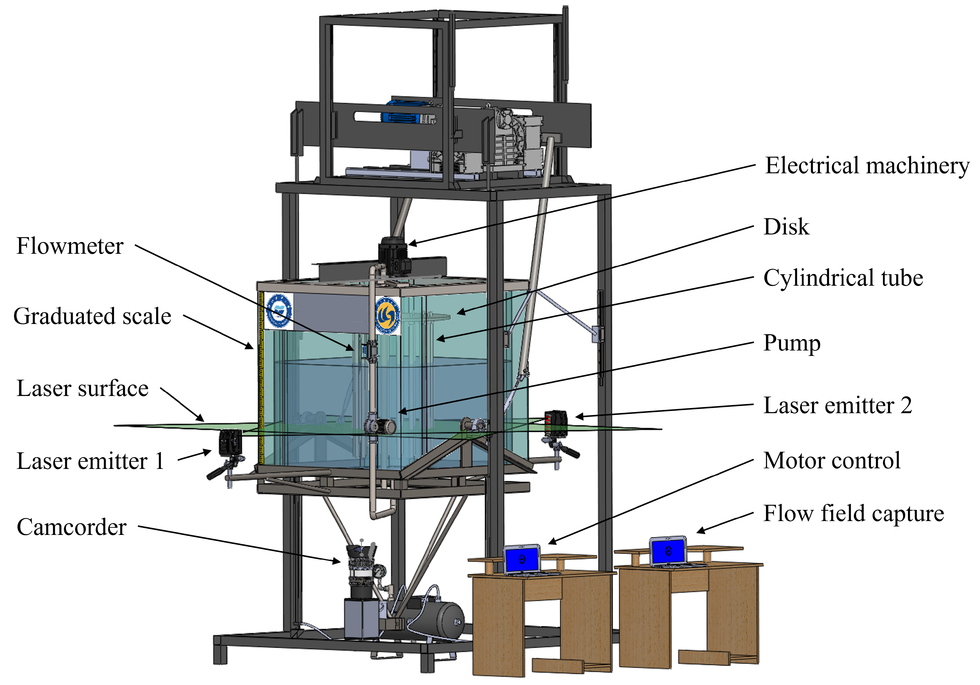
2.1. Experimental Setup

The experimental system comprised three subsystems: a circulation system, a data acquisition system, and a fish school simulation system.

The experiment began with the activation of the circulation system. The outlet at the bottom of the tank was connected to the inlet via a pipe, thereby forming a closed-loop flow path. The target flow rate was adjusted using a regulator installed on the pipe, while the jet angle was configured using a 360° dial located at the pipe inlet to establish the initial flow environment. Prior to each trial, the circulation system was operated for 15 min to ensure the establishment of a steady flow field.

After the flow field had stabilized, the fish simulation system was activated. Under precise motor control, the system rotated counter to the main flow direction to simulate the annular flow field induced by fish swimming. The motor’s rotational speed and direction were governed by a pre-programmed controller, which specified different settings according to the experimental requirements. During the simulation, flow disturbances generated by the fish simulation system were superimposed onto the base flow from the circulation system, resulting in a complex, composite flow field.

Once both the circulation and fish simulation systems had reached stable operating conditions, the data acquisition system was activated. The laser transmitter of a Particle Image Velocimetry (PIV) system was calibrated to align with the same measurement plane on both the front and rear sides of the tank. A high-resolution CCD camera was mounted beneath the tank to record the motion of tracer particles within the laser sheet in real time. Throughout the experiment, the data acquisition system continuously monitored variations in the flow field, while the CCD camera transmitted the captured image data to a computer for real-time processing. Image analysis was employed to compute the displacement and velocity of tracer particles, thereby enabling the extraction of velocity distributions and other essential flow field parameters. The experiments were conducted in a tank whose internal configuration was modified by adding or removing deflector baffles. To ensure reliability and reproducibility, each experimental condition was conducted in five replicates. The experimental setup is illustrated in Figure 1.

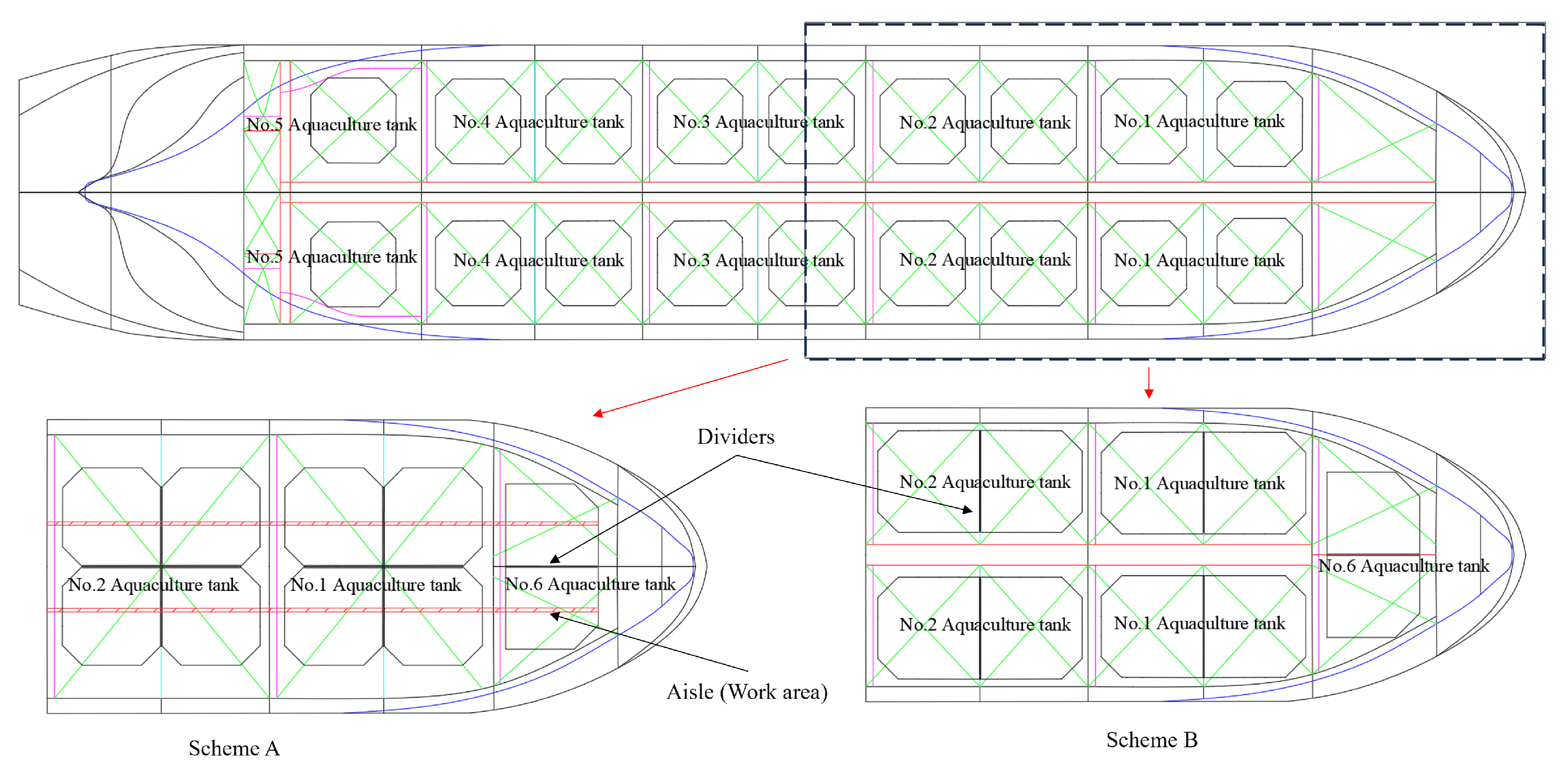
2.2. Aquaculture Tank Setup

A 1 m³ square tank was modified by installing sealed acrylic boards (1 m long, 0.28 m wide, and 0.02 m thick) at its corners. The water level was maintained at 0.4 m. The jet pipe was 1.1 m in length, 0.002 m thick, and had a diameter of 0.02 m. It was positioned 0.05 m above the tank bottom, with outlet holes (0.004 m radius) spaced every 0.08 m along its vertical length. The outlet was located at the center of the bottom, with a radius of 0.004 m. A circular arc-shaped tank was constructed by replacing the corner acrylic panels with curved ones. The final tank configuration, including the arc-shaped variant, is shown in Figure 2.

The flow rate in the pipe was regulated by a flow meter, and the corresponding conversion from volumetric flow rate to flow velocity is given by Equation (1):

$$v={\displaystyle \frac{Q}{\mathrm{60,000}\pi r^2}}$$

(1)

where v is the flow velocity (m/s), Q is the flow rate measured directly by the flow meter (L/min), and r is the radius (m).

In aquaculture, the characteristics of the flow field in aquaculture tanks have a crucial impact on the survival environment and growth condition of cultured organisms. To investigate how tank geometry influences flow dynamics, this study focused on two representative shapes: octagonal and circular arc. The octagonal tank featured multiple corners and a regular polygonal structure, while the circular arc tank presented a smooth curved profile. These contrasting geometries offer valuable comparative insight into flow field variations.

In modern aquaculture, vessel-based farming systems have emerged as a new operational model, exemplified by the “Guoxin 1” vessel, which utilizes octagonal aquaculture tanks. However, the structural constraints of the vessel significantly influence the layout and spatial utilization of aquaculture tanks. To maximize the use of limited onboard space, the aquaculture compartments in this study were enlarged to increase the effective farming volume while ensuring rational placement at both the bow and stern of the vessel (layout illustrated in Figure 3).

By removing the deflector baffles from the two basic tank geometries, four additional aquaculture tank configurations were derived through structural modifications tailored to aquaculture requirements. This approach enables a more comprehensive investigation of how different tank geometries and structural designs influence flow field characteristics.

Detailed diagrams of the structural configurations of the aquaculture tanks are illustrated in Figure 4 and Figure 5, including the octagonal shape, circular arc shape, and four additional shapes derived by removing the boundary baffles. An analysis of Figure 4 provides us with an intuitive understanding of the geometric features and boundary conditions of the various tank configurations, providing essential foundational information for subsequent flow field analysis.

The experiments were conducted using flow field results captured by a high-speed camera, and the images were automatically processed using the PIV system. The collected data were post-processed using Python 3.13 to standardize the flow field and facilitate clearer visualization of flow phenomena. Between experiments, the incubation tank was paused for 20 min to allow the liquid to return to a static state, minimizing interference between successive trials. Each round of data acquisition began 10 min after the start of the experiment and lasted for 5 min.

In the flow field image shown in Figure 6, an anomaly appears in the upper right region where data are missing. This is because the camera is positioned below the tank, and circulation pipes obstruct its line of sight, preventing complete capture of the flow field and resulting in a shaded area in the velocity vector diagram.

3. Results and Discussion

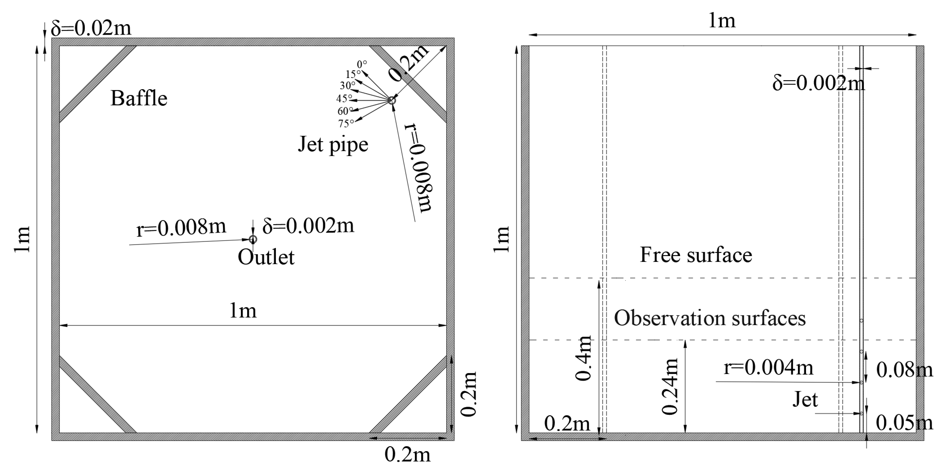
3.1. Octagonal Aquaculture Tanks

Taking the octagonal aquaculture tank as a reference case, this study conducted an in-depth investigation of the flow field characteristics associated with three different tank configurations. To examine the effects of jet angle and jet velocity on the flow field under steady-state conditions, the average flow velocity was calculated. As illustrated in Figure 7, when the jet velocity was set to 1.5 m/s, the flow fields at six different jet angles (0°, 15°, 30°, 45°, 60°, and 75°) were examined under steady-state conditions.

A sampling frequency of 30 Hz was used during data acquisition, and the figure shows that the average flow velocity remained consistently stable. This confirms that the flow field within the tank had reached a steady state.

To quantify measurement variability, the standard deviation was used to assess the dispersion of the measured flow velocities. The average flow velocity at seven jet angles (as shown in Figure 8) was computed. The maximum error and standard deviation over a 5 s interval were calculated using the stabilized average flow field as a reference.

The standard deviation Equation (2) is as follows:

$$\sigma =\sqrt{{\displaystyle \frac{1}{n}}{\displaystyle \sum _{i=1}^n}{(x_i-\mu )}^2}$$

(2)

The maximum deviation in the graph reflects the maximum degree of deviation of individual measurements from the mean. The standard deviation quantifies the overall spread of measurement values around the mean. The results in the graph show that the maximum deviation is 4.9% at 60°, while the standard deviations are all below 1.8%, which indicates that the experiments are reproducible and the measurements are reliable.

The average velocity $v_{avg}$ represents the average result of the entire flow field velocity and is given by the following Equation (3):

$$v_{avg}={\displaystyle \frac{1}{n}}\sum _{i=1}^n{v}_i$$

(3)

where $v_i$ denotes the instantaneous velocity of the particle at that moment.

Additionally, to better describe the vortex phenomenon observed during the experiment and in the aquaculture vessel (as shown in Figure 9), a trend index $\gamma$ is introduced:

$$\gamma =1-{\displaystyle \frac{1}{n}}\sum _{i=1}^n{\displaystyle \frac{|v_{r,\mathrm{avg}}-v_{r,i}|}{v_{r,\mathrm{avg}}}}$$

(4)

The value of $\gamma$ in in the range of (0, 1); it is considered that the larger the result of $\gamma$, the more obvious the trend of the flow field, and the better the aquaculture effect. $v_{r,avg}$ indicates the average flow velocity of a circle of point data under the radius, with the exit position in the aquaculture tank as the center of the circle, and $v_r$ indicates the velocity of each point under the radius.

In this study, the length corresponding to the side of the aquaculture tank was determined to be the maximum radius using the location of the center of the circle at the exit of the aquaculture tank as the center point. Subsequently, 50 flow coils were drawn inside the aquaculture tanks according to equal radius spacing. This is shown in Figure 10.

To investigate the effects of varying jet angles and velocities on the flow field of the octagonal aquaculture tank in the stationary state, 30 experimental conditions (as listed in

Table 1. Experimental setup in the stationary state of the incubation tank.

Case	Jet Velocity (m/s)	Jet Angle (°)
1	0.5	0, 15, 30, 45, 60, 75
2	1	0, 15, 30, 45, 60, 75
3	1.5	0, 15, 30, 45, 60, 75
4	2	0, 15, 30, 45, 60, 75
5	2.5	0, 15, 30, 45, 60, 75

) were conducted. The average flow velocity and flow trend index were computed, and the results are presented in Figure 11. The results show that when the jet angle increases from 0° to 45°, the average flow velocity rises correspondingly. However, with further increases in the jet angle beyond 45°, the average flow velocity exhibits a decreasing trend.

When the jet angle is in the 0° to 15° range, the incident water will collide with the wall of the breeding pool and be accompanied by the refraction and reflection of the water quality points, which will make the water body experience a large loss of energy. As the jet angle increases to 30°–45°, the trajectory of the jet stream lengthens before it reaches the wall, reducing the interaction and energy dissipation caused by direct impact. At higher jet angles (60°–75°), as shown in Figure 12, the jet flow is directed more toward the central region rather than the walls, reducing the circulation zone and leading to the formation of large dead-water areas.This occurs due to an uneven distribution of flow velocity and pressure within the tank, with higher pressure and velocity concentrated near the jet inlet.This flow rate differential induces rotational motion, which eventually leads to the formation of vortices. Additionally, pressure gradients can cause fluid to move from high- to low-pressure regions, and the resulting flow instability further contributes to vortex formation. As a result, both forward and reverse circulations are generated, leading to the most unfavorable flow field conditions within the tank.

In the longitudinal comparison at a constant jet velocity, the average flow velocity reaches its peak at jet angles of 30° and 45°. Furthermore, when the jet velocity reaches 2.5 m/s, the change in the average flow velocity becomes significantly more pronounced compared to the other jet velocity conditions. This phenomenon may indicate that with an increase in the jet velocity, the flow field average velocity is not linearly increasing, and its change trend becomes more significant.

In an actual aquaculture scenario, fish typically exhibit circular swimming patterns around the center of the tank. Based on the above experimental results, it can be inferred that under high jet velocities, selecting a smaller jet angle contributes to a more stable flow field, which is more conducive to fish aquaculture.

Specifically, the side of the octagonal aquaculture tank adjacent to the jet inlet was analyzed. Two additional configurations were derived by removing one and two deflector baffles. The jet angle was gradually increased from 0° to 75° with a constant jet velocity of 2 m/s, with each increment of 15°, covering a total of 12 different conditions (

Table 2. Experimental setup of aquaculture tanks before and after disassembly.

Case	Jet Velocity (m/s)	Jet Angle (°)
R0	2	0, 15, 30, 45, 60, 75
R1	2	0, 15, 30, 45, 60, 75
R2	2	0, 15, 30, 45, 60, 75

). The corresponding velocity vector distributions are illustrated in Figure 13, Figure 14 and Figure 15.

It can be seen that the flow field is more turbulent in the aquaculture tank with two deflectors removed compared to the case with one deflector removed. This difference is particularly noticeable at a jet velocity of 2 m/s and a jet angle of 75°.

To further quantify and analyze the impact of deflector removal on the flow field, 18 sets of experimental data were collected at a jet velocity of 2 m/s before and after removing the corner deflector baffles of the aquaculture tank. The results are presented in Figure 16.

In aquaculture, the fluid environment within the vessel is critical to the survival and growth of cultured organisms, and the configuration of deflector baffles is essential for optimizing this environment. Figure 16 presents the effects of different deflector removal scenarios on the flow field of aquaculture tanks, where “R” stands for “remove the Baffle” and “R0” denotes the initial state without removing the deflector.

When the deflector baffle remains intact, it alters the internal flow pattern of the aquaculture tank. The deflector induces a directional or circulatory flow within the tank. This guided flow enhances the overall fluid velocity. Under such orderly flow conditions, the flow field exhibits a more pronounced and stable trend. The velocity distribution becomes more uniform, with consistently high and stable values across the tank. This provides a relatively stable and suitable water flow environment for cultured organisms, which is conducive to their survival and growth.

However, when the two deflector baffles were removed, the fluid environment in the aquaculture tank changed significantly. The flow path of the fluid became more complex and disordered. Compared to the configuration with intact deflectors, the removal of two baffles resulted in a substantial reduction in the average flow velocity and a less distinct flow trend. The original uniform and stable flow velocity distribution was disrupted, regional velocity differences increased, and turbulence in the flow field intensified. This change may have adversely affected the survival environment of cultured organisms. Therefore, between the two schemes based on the octagonal aquaculture tank, Scheme A demonstrates superior flow characteristics compared to Scheme B.

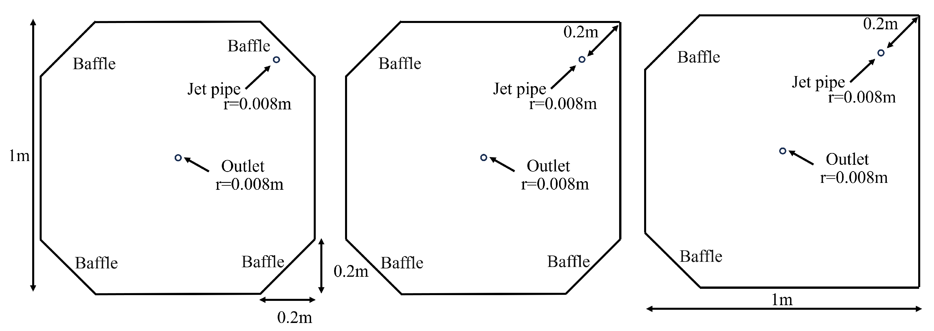
3.2. Arc-Shaped Aquaculture Tanks

Following the same experimental methodology, the study was extended to a culture tank with a circular deflector baffle. The flow fields were compared across three configurations: with the deflector intact, with one deflector removed, and with two deflectors removed.

In this experiment, 30 sets of trials were conducted for the arc-shaped aquaculture tanks with reference to the experimental conditions listed in Table 1. The results are presented in Figure 17.

Compared to arc-shaped tanks, octagonal tanks exhibit higher average flow velocities at larger jet angles (30° and 45°), whereas arc-shaped tanks show higher velocities at smaller jet angles (0° and 15°). The enhanced flow efficiency in octagonal tanks is attributed to their angular, polygonal geometry, which facilitates directional circulation at specific jet angles. In contrast, arc-shaped tanks rely on their smooth wall surfaces to reduce collision losses at small jet angles, thereby improving flow velocity. Water circulation in octagonal tanks is strongly dependent on the synergy between the structural geometry and jet angle.

From the perspective of flow field trend analysis, the $\gamma$-value serves as an important indicator of flow stability and structural characteristics in arc-shaped tanks, exhibiting a clear and consistent pattern. At a jet angle of 0°, the $\gamma$-value is more stable than at other angles. This suggests that at a jet angle of 0°, the flow field in the arc-shaped tanks is relatively stable, with consistent flow patterns and minimal fluctuations. As the jet angle increases, the $\gamma$-value shows a clear downward trend. This indicates that increasing the jet angle reduces flow stability, leading to more complex and unstable patterns, including enhanced vortex formation and turbulence, which, in turn, increase energy dissipation and variability in flow field characteristics. In the octagonal tanks, on the other hand, the $\gamma$-value is minimally stabilized at about 0.8 with the flow velocity when the jet angle is 45°.

In addition, the $\gamma$-value of the circular arc-shaped aquaculture tanks under the condition of low jet velocity is significantly larger than the value in the other cases. This suggests that at low jet velocities, the flow field in circular arc-shaped tanks can maintain a more stable structure and trend. This may be attributed to the lower energy of the water flow at low velocities, making it more susceptible to confinement and guidance by the tank walls, thereby facilitating the formation of a relatively stable flow field. Under the condition of high jet velocity, the energy of the water flow is larger, and it is easier to break through the constraints of the circular arc-shaped bulkhead, which leads to a decrease in flow field stability and a reduction in the $\gamma$-value.

Figure 17 shows the average flow velocity and the corresponding flow field trends for the arc-shaped tanks presented in Figure 18, Figure 19 and Figure 20 for the three conditions of no deflector removal, the removal of one deflector, and the removal of two deflectors. The phenomena presented in these three conditions are significantly different from the performance of the octagonal culture tank in the same three conditions.

In the low jet angle range (0°–30°), the average flow velocity shows a significant decreasing trend with an increase in the number of removed deflectors. With the gradual removal of the deflectors, the flow is less guided and constrained, which leads to a decrease in the mean flow velocity. At this stage, the R0 curve in Figure 17 (no deflectors removed) shows the highest average flow velocity, followed by R1 (one deflector removed) and R2 (two deflectors removed) with the lowest value. This trend aligns with the main text’s discussion stating that “the weakening of guiding and constraining effects leads to a reduction in average flow velocity”. It also visually confirms that the average flow velocity under low jet angles decreases significantly with the removal of deflectors. The conclusion that the number of deflectors affects the mean flow velocity at low jet angles is supported.

In contrast, the trend differs under high-jet-angle conditions. When one deflector is removed, the mean flow velocity remains comparable to that in the configuration without deflector removal. This suggests that at high jet angles, the removal of a single deflector has a limited effect on the overall flow velocity. The energy of the high-speed jet likely compensates for the lack of guidance provided by the deflector. A similar trend is also observed in the flow field characteristics—that is, the flow pattern remains comparable to that observed with the deflector intact. In Figure 17, the R0 and R1 curves are closely aligned at high jet angles, indicating that both the average flow velocity and flow trend remain similar regardless of the removal of a single deflector. This provides intuitive evidence supporting the main text’s conclusion that removing a single deflector has minimal impact under high jet angles, and further validates the conclusion that a single deflector has a limited effect on flow dynamics at high jet angles.

When both deflectors are removed, the flow field turbulence increases significantly under high-jet-angle conditions. This trend is clearly illustrated in Figure 21. In Figure 17, the R2 curve (two deflectors removed) deviates significantly from the R0 (no deflector removed) and R1 (one deflector removed) curves at high jet angles, showing large fluctuations and no consistent pattern in the average flow velocity. This visually demonstrates the increased turbulence resulting from the removal of two deflectors, consistent with the main text’s discussion: “The degree of turbulence of the flow field is greatly increased when removing the two deflector plates”. This observation provides important guidance for optimizing the structural design and operational control of aquaculture tanks. Moreover, since the impact on the flow field is minimal when only one deflector is removed, Scheme A proves to be more advantageous, as clearly demonstrated by the close alignment of the R0 and R1 curves in Figure 17. This further supports the conclusion that Scheme A is the superior configuration.

3.3. Circular Fish School Swimming Patterns

In aquaculture, understanding the swimming patterns of fish and the resulting flow field characteristics is crucial for optimizing rearing conditions and enhancing production efficiency. Fish movement in a real natural environment is analyzed (shown on the left of the Figure 22). In natural waters, fish often exhibit a unique circular swimming pattern. This circular movement is not random and disorderly, and the fish move in a coordinated circular pattern and in the opposite direction to the flow field to ensure better foraging, the avoidance of predators, and maintenance of the stability of the group. Each fish has a relatively fixed position and swimming rhythm in the ring formation.

Reproducing circular swimming patterns with live fish is more difficult due to the limitations of laboratory experiments, as fish usually swim against a steady current, as shown on the left of Figure 22. Moreover, the size and behavior of each fish cannot be accurately modeled. Therefore, these characteristics are highly simplified when reproducing the swimming behavior of a school of fish in a laboratory experiment. When fish swim in a circle, they are assumed to be equally spaced in the circumferential direction and closely spaced in the vertical direction.

The device consisted of a central disc placed within the culture tank and a surrounding rim structure. Along the edge of the disc (0.5 m from the center, forming a circle of 0.5 m in diameter), 18 evenly spaced cylindrical tubes with a diameter of 0.02 m were mounted [25]. Polyvinyl chloride (PVC) pipes were used to simulate the presence of fish cultured in cages. The pipe diameter was determined based on the maximum body length (18–22 cm) of one-year-old greater yellow croaker, applying a 1:10 downsizing ratio of the actual culture compartment. Each pipe was sealed with PVC caps, with one end fitted with a screw for attachment to a wooden tray. Additionally, the pseudo-fish school structure was rigid, preventing the replication of the undulating swimming motion observed in live fish.

In order to simulate the annular flow field formed by the fish, the disc was able to rotate in the opposite direction to the fluid in the culture tank through the precise control of the motor. When the disk started to rotate, the circular tube moved along with it and interacted with the surrounding fluid, thus creating a flow field in the culture tank similar to that created by the circular movement of the fish. Because the shape and arrangement of the tubes could approximate the distribution and movement of fish in the water to a certain extent, the rotational movement of fish in the actual environment could be simulated by letting the disk drive the tubes to rotate. The direction of the tube was set to be opposite to the direction of the flow field, which is a more realistic reflection of the movement of the fish and their interaction with the water flow.

In the process of calculating and analyzing the experimental data, the existence of the round tube will lead to a special flow pattern in the flow field around it, and a high velocity region will be formed near the round tube.To ensure the accuracy and reliability of the experimental results, the flow disturbances caused by the tubes and the associated high-velocity regions were excluded from the analysis. This approach effectively isolated the flow field characteristics generated by fish movement, and the computational domain is illustrated in Figure 23.

Figure 24 shows the flow field of the fish simulator under various jet angles. In the experimental process, the jet velocity was set at 2.5 m/s, and the rotational speed of the fish was stabilized at 3 rpm. Based on this, the study was carried out for different jet angles. By changing the jet angle, a variety of possible water flow situations in the actual aquaculture environment were simulated.

The observed flow field exhibits characteristics similar to those found in the airspace experiments. The circular tubes, as key elements influencing the flow field, exert a consistent effect on fluid dynamics. This suggests that both the fish simulation setup and the airspace experiments produce similar flow field characteristics across different experimental conditions.

Analyzing the experimental results presented in Figure 25, it is found that the trend of the mean flow velocity in this flow field shows a high degree of consistency with the trend observed in the airspace. The mean flow velocity reaches its peak at a jet angle of 15°. This indicates that energy transfer and conversion efficiency are likely optimized at this specific jet angle, thereby maximizing the mean flow velocity. However, when compared with the airspace experiments, the peak mean flow velocity in the fish simulation decreased by 66.875%. This significant reduction suggests that the presence of the fish population imposes considerable resistance on the fluid flow, consuming substantial energy during transmission and thereby reducing the mean flow velocity. A significant decrease in the flow field’s trend index is also observed in the fish simulation experiments, averaging approximately 37.5%. The trend index typically reflects the spatial uniformity and stability of the flow field. Its decline indicates that the presence of fish disrupted the stability and regularity of the flow field. The swimming of fish may trigger localized turbulence and vortexing, making the flow of fluid more complicated and disordered, thus leading to a decrease in the trend index.

Tail eddies generated by the fish simulator consume flow field energy, as evidenced by the reduction in mean flow velocity. These eddies require energy to form and sustain, which is drawn directly from the flow field. As tail vortices continuously form and evolve, they extract significant energy from the flow field, thereby reducing the overall flow velocity. The presence of tail vortices induces localized turbulence, disrupting the originally stable and uniform flow and causing sharp variations in the flow direction and velocity, ultimately leading to a decline in the trend index. These vortices also alter the flow paths and introduce disturbances to the surrounding fluid, preventing it from following its original trajectory, which further contributes to complex flow patterns and a reduction in the trend index.

Figure 26 shows the flow field comparison results under different jet velocities, with the circular tube’s rotational speed controlled at 3 rpm. At a jet angle of 45°, the results indicate that increasing the jet velocity leads to an expansion in the high-velocity region in the flow field.

By comparing the mean flow velocity and trend index shown in Figure 27, a clear increasing trend in mean flow velocity can be observed with the gradual increase in jet velocity. This result indicates that jet velocity largely governs the fluid motion in the flow field; higher jet velocities impart more energy to the fluid, thereby driving faster flow.

When the jet velocity reaches 2.5 m/s, the mean flow velocity in the tank drops significantly—by 71.1%—compared to that observed in the airspace condition. This demonstrates that the presence of fish significantly influences the overall mean flow velocity. The trend index exhibits an overall upward trend. Higher jet velocities may facilitate the formation of structured flow patterns, thereby increasing the trend index.

However, despite this upward trend, the average trend index decreases by 34.7% across the four jet velocities. This suggests that the circular movement of fish disrupts the flow field pattern, resulting in a decrease in mean flow velocity.

By varying the rotational speeds of the discs, the swimming behavior of annular fish schools in a controlled flow environment was simulated, as shown in Figure 28. The disc rotation speeds ranged from 3 rpm to 7 rpm. As the rotational speed increased, the rotating region became progressively darker, indicating a higher local flow velocity. Notably, the disc rotation was set opposite to the primary flow direction in the tank. This reverse rotation setup further increased the complexity of the flow field and more accurately mimicked the conditions found in actual aquaculture environments.

To more precisely analyze the impact of the flow field characteristics on the simulated fish swimming speed, the high-velocity region induced by the circular tubes was excluded from the analysis. A clear decreasing trend in the high-velocity region of the flow field was observed. This trend suggests that as the circular disc’s rotational speed increases, the overall extent of the high-velocity region decreases, although local flow velocity near the rotating disc remains elevated.

As shown in Figure 29, the degree of flow field disturbance increases significantly with increasing rotational speed. Higher rotational speeds give rise to more complex fluid dynamic phenomena, including vortex formation and intensified turbulence. These phenomena interact to disrupt the previously stable flow field, thereby altering its overall structure and flow characteristics.

The average flow velocity tends to 0 as the rotational speed increases, which indicates that the fluid motion in the flow field gradually slows down, and as the flow power weakens, the trend index also shows a trend of decreasing with an increase in rotational speed. This means that the flow field almost presents a stationary flow state. In this state, the fluid in the flow field almost no longer exhibits an obvious macro-flow, and the relative position of the fluid in each region changes very little.

4. Conclusions

This study draws the following conclusions based on the investigation of flow field characteristics in aquaculture tanks with different structural configurations and under two distinct scenarios, including simulations involving fish movement:

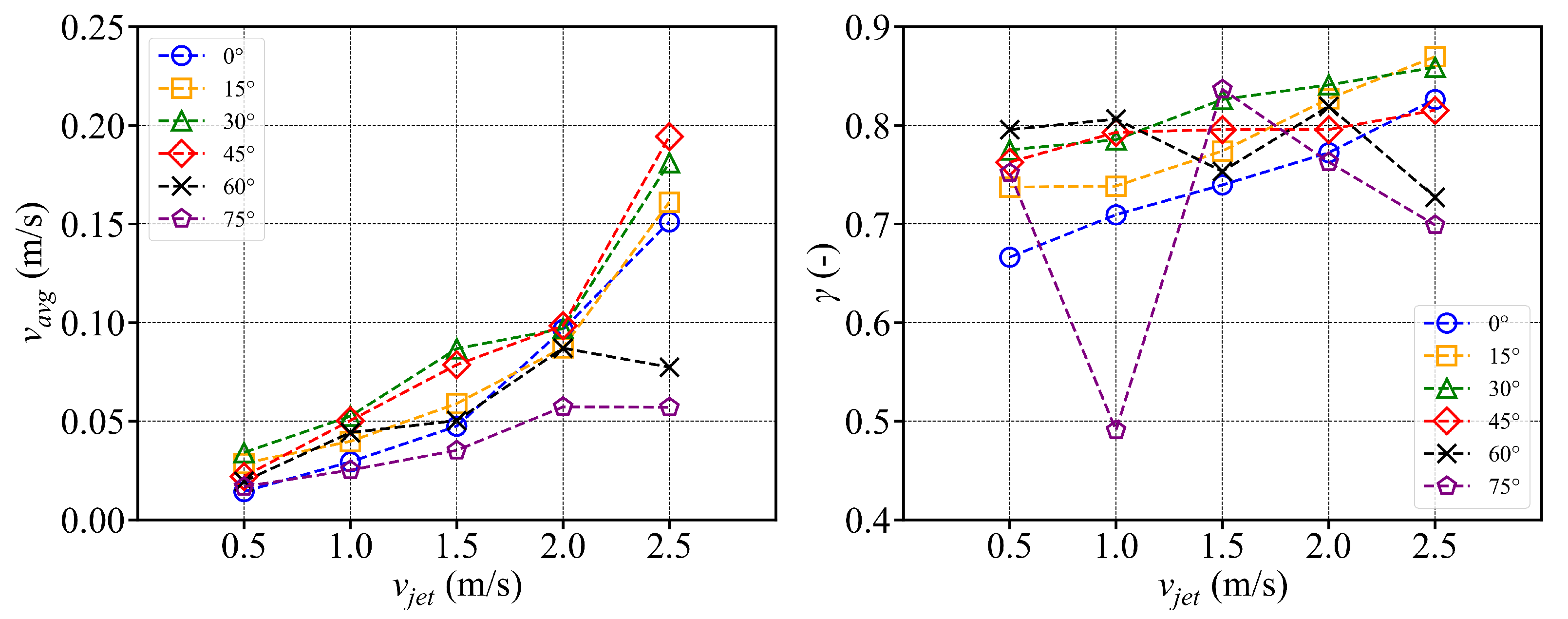
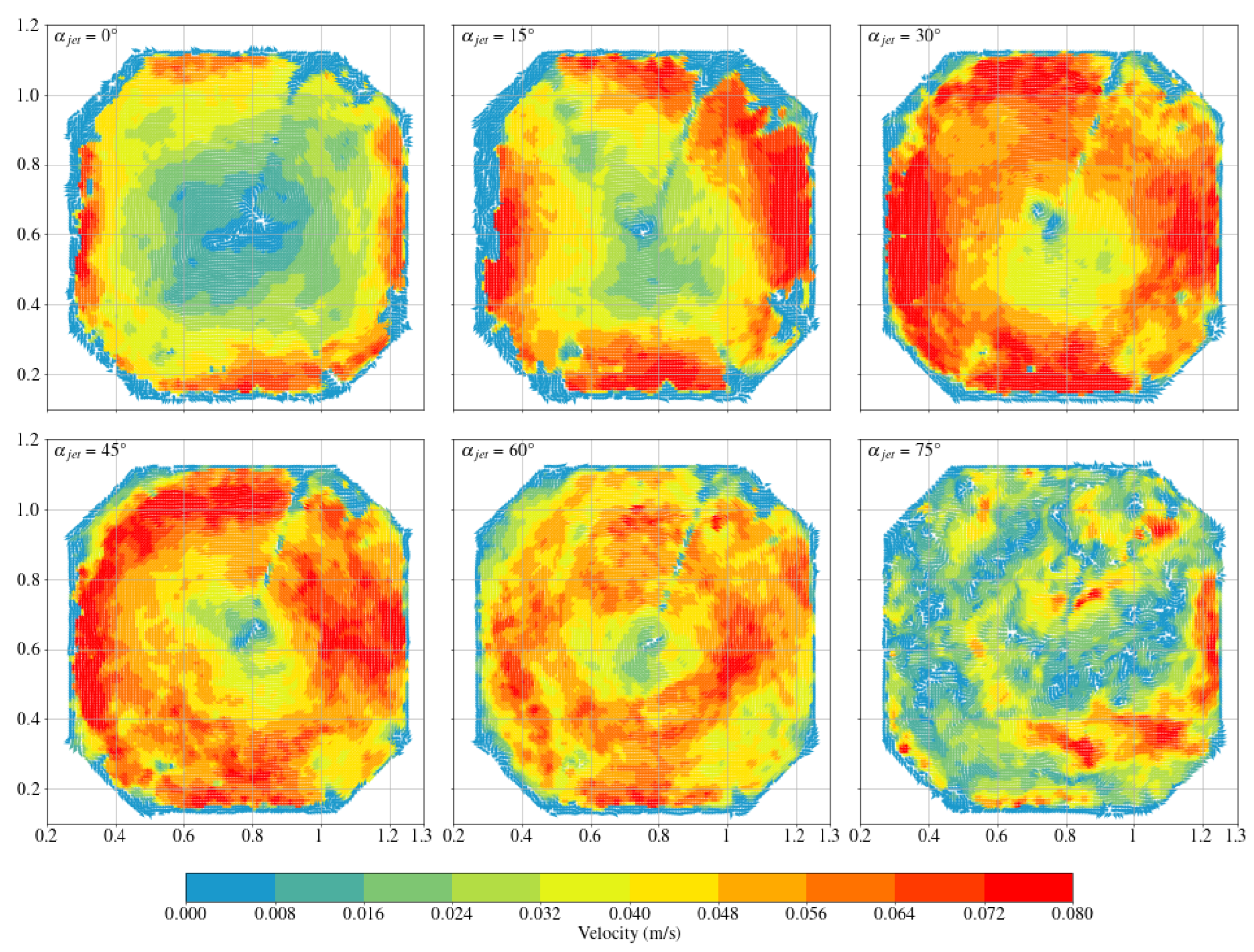
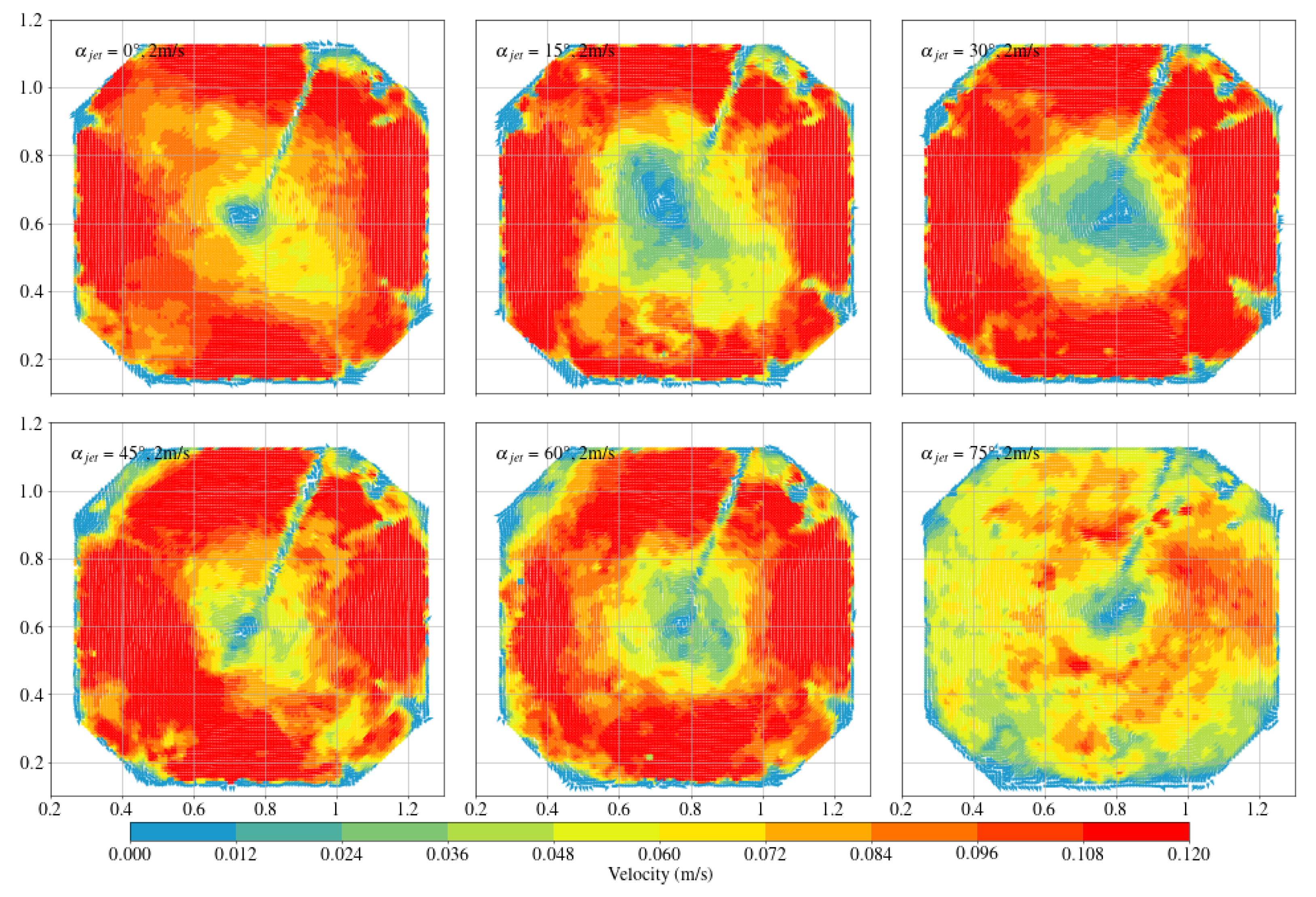
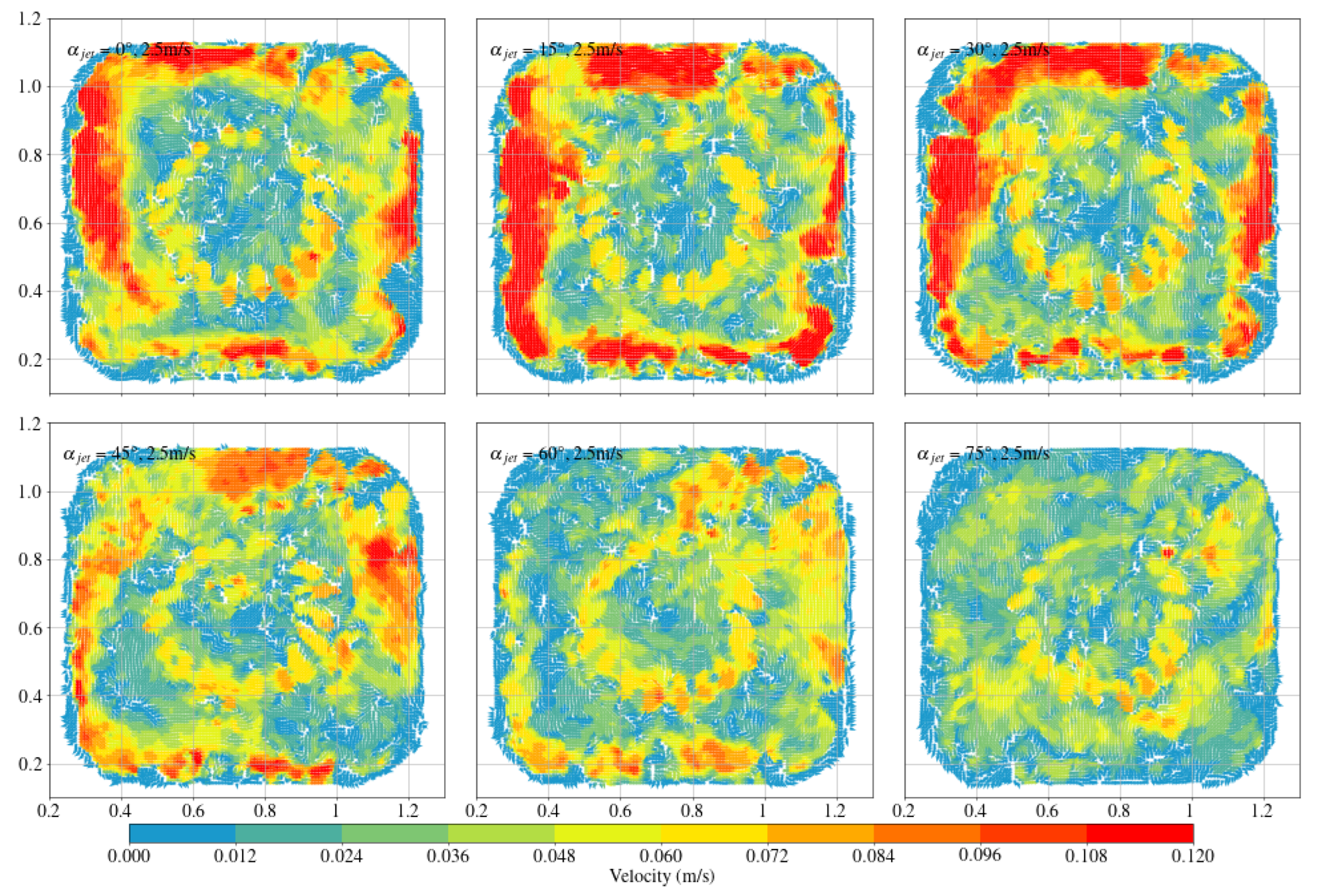
• In the octagonal aquaculture tank, the mean flow velocity increases with jet angle in the range of 0° to 45°, but begins to decline as the angle increases further. The flow velocity peaks at jet angles of 30° and 45°, with particularly significant changes observed at a jet velocity of 2.5 m/s. At smaller jet angles, the flow trend becomes more pronounced as the flow velocity increases. The $\gamma$-value reaches its maximum at 30°, while at 45°, the trend is least sensitive to changes in jet velocity. No consistent trend in $\gamma$-value is observed at higher jet angles (60° and 75°), indicating increased instability. Removing two deflector baffles leads to greater turbulence than removing one. Retaining the deflectors promotes the formation of stable and directional flow, with high mean flow velocity, a clear trend, and uniform distribution—conditions beneficial to fish growth. In contrast, removing both deflectors significantly reduces the flow velocity, disrupts trend clarity, and increases turbulence, which may adversely affect aquaculture.
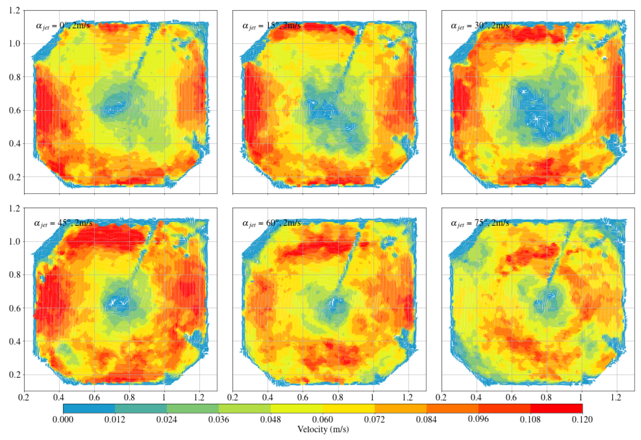
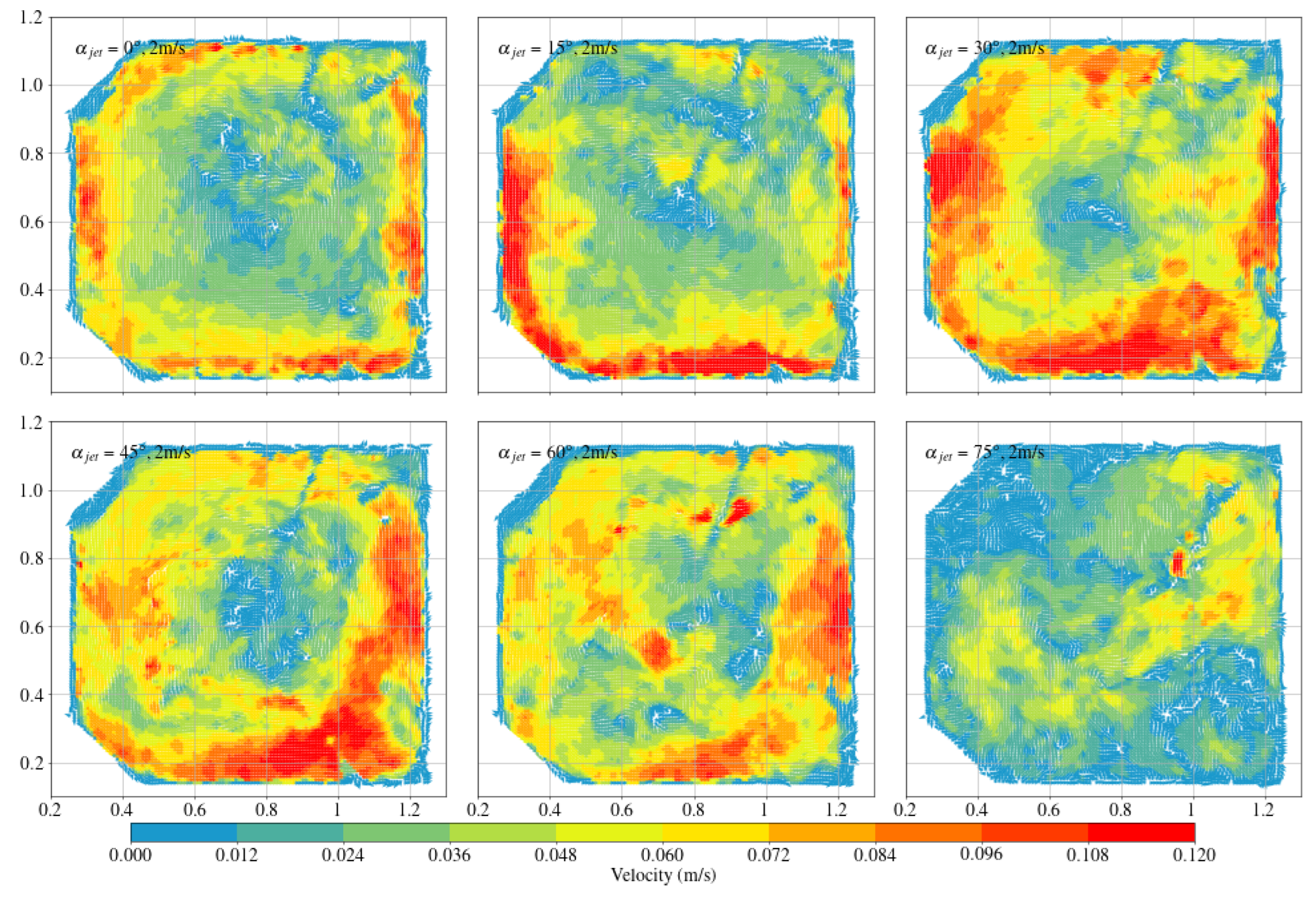
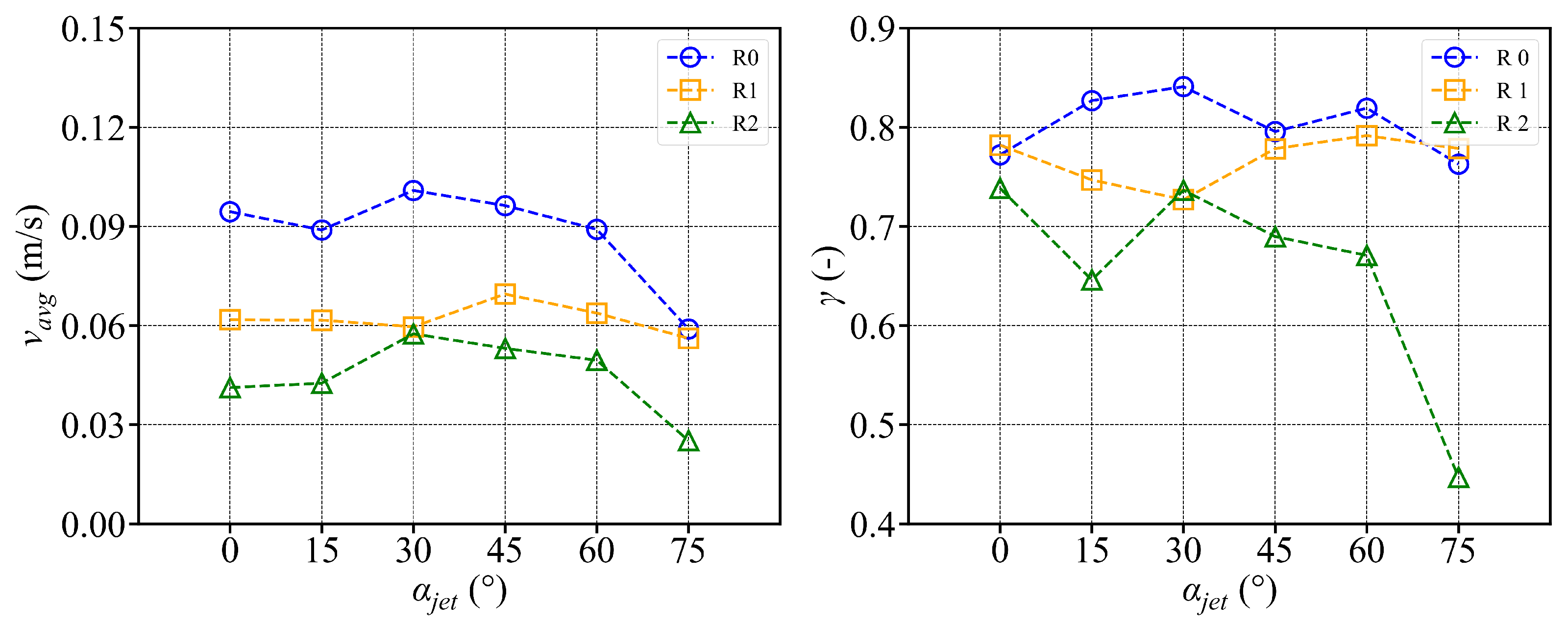
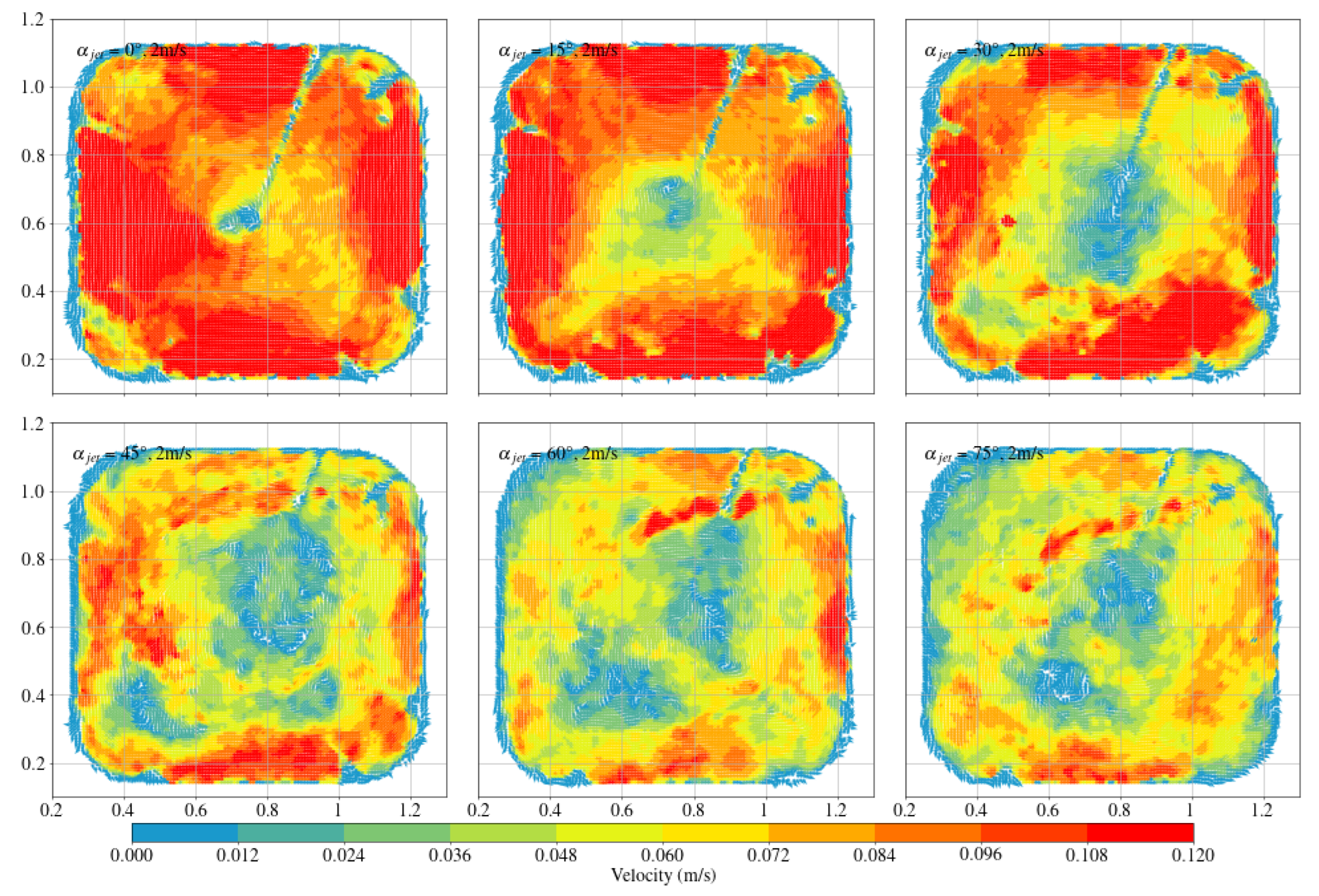
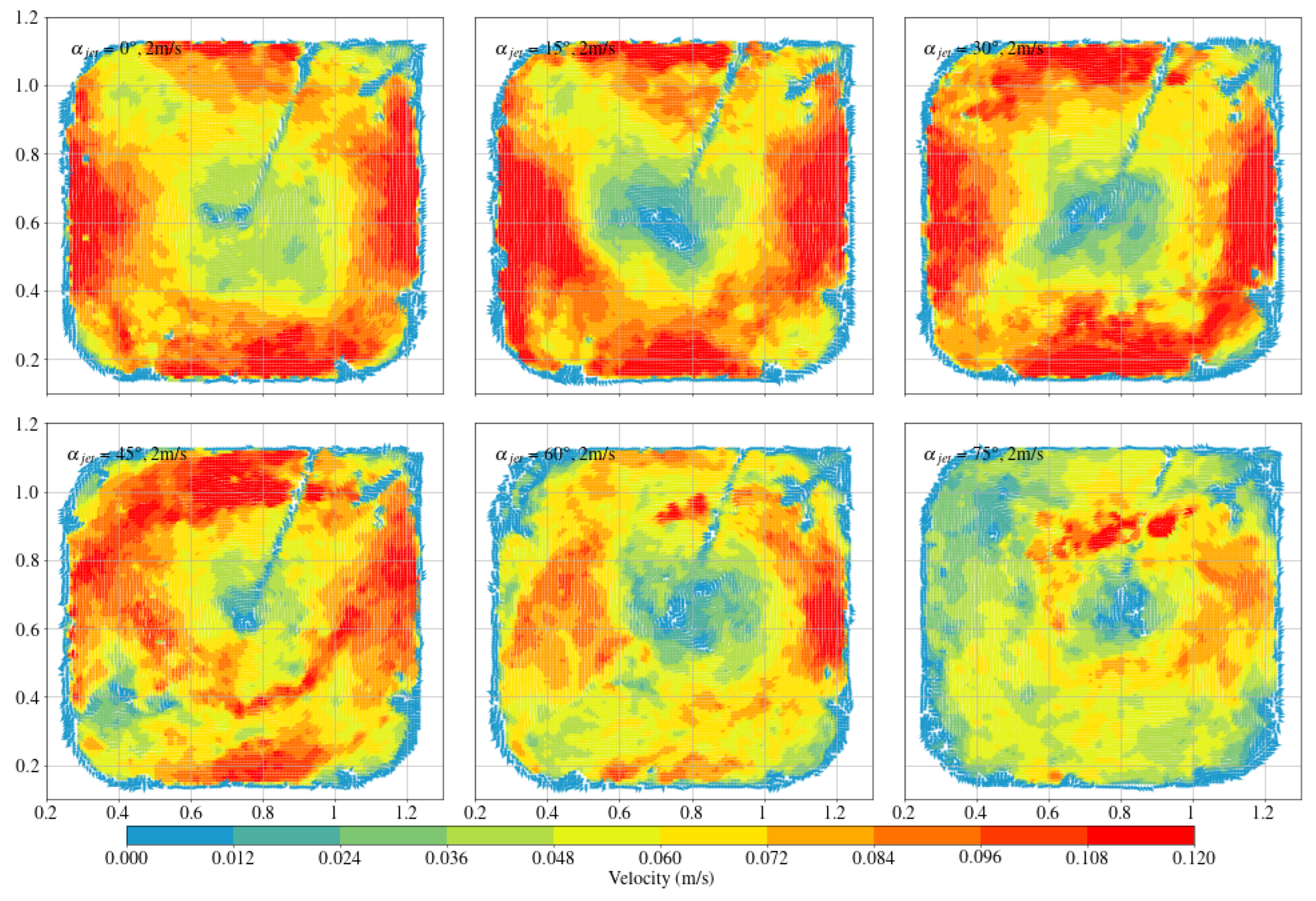
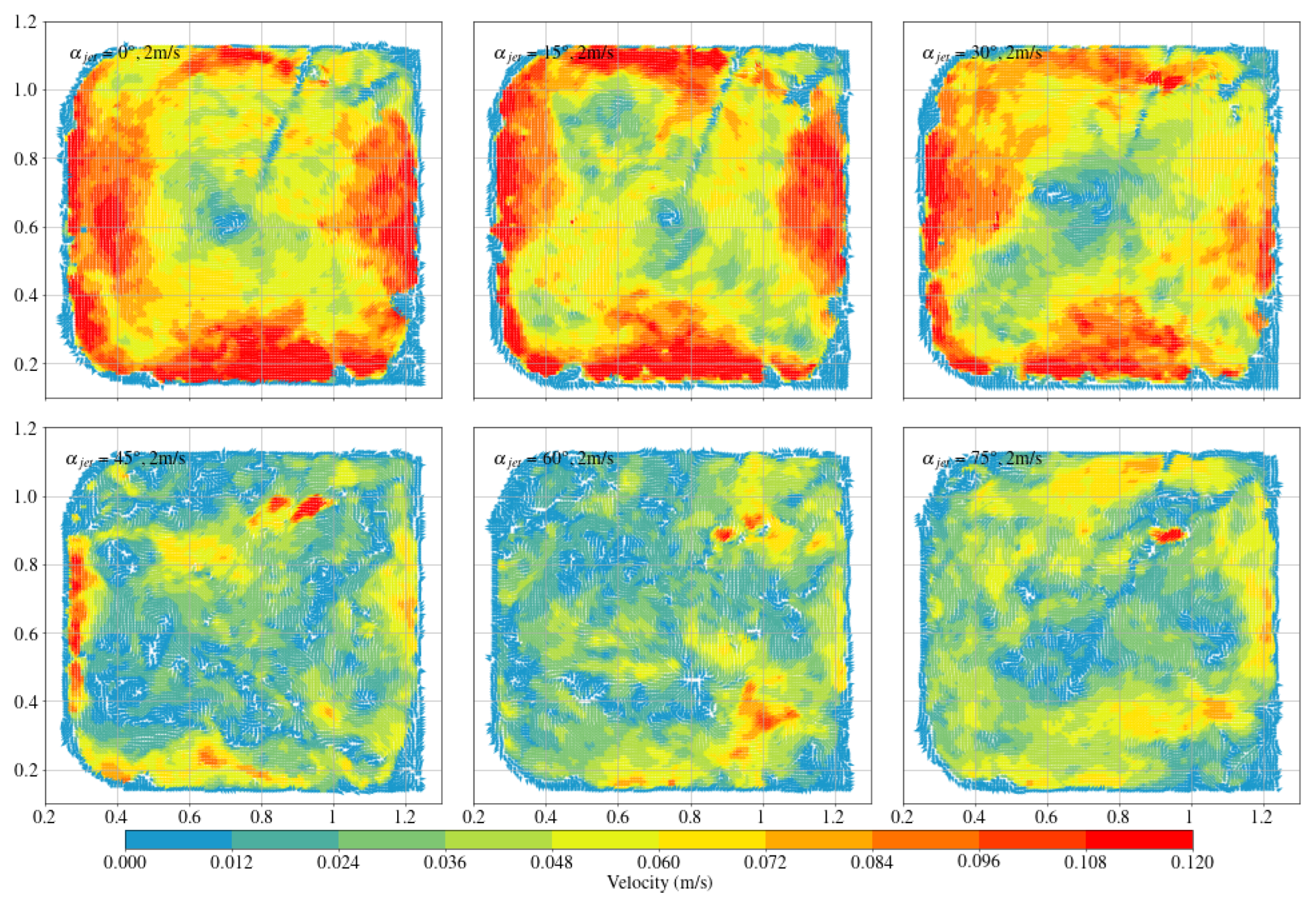
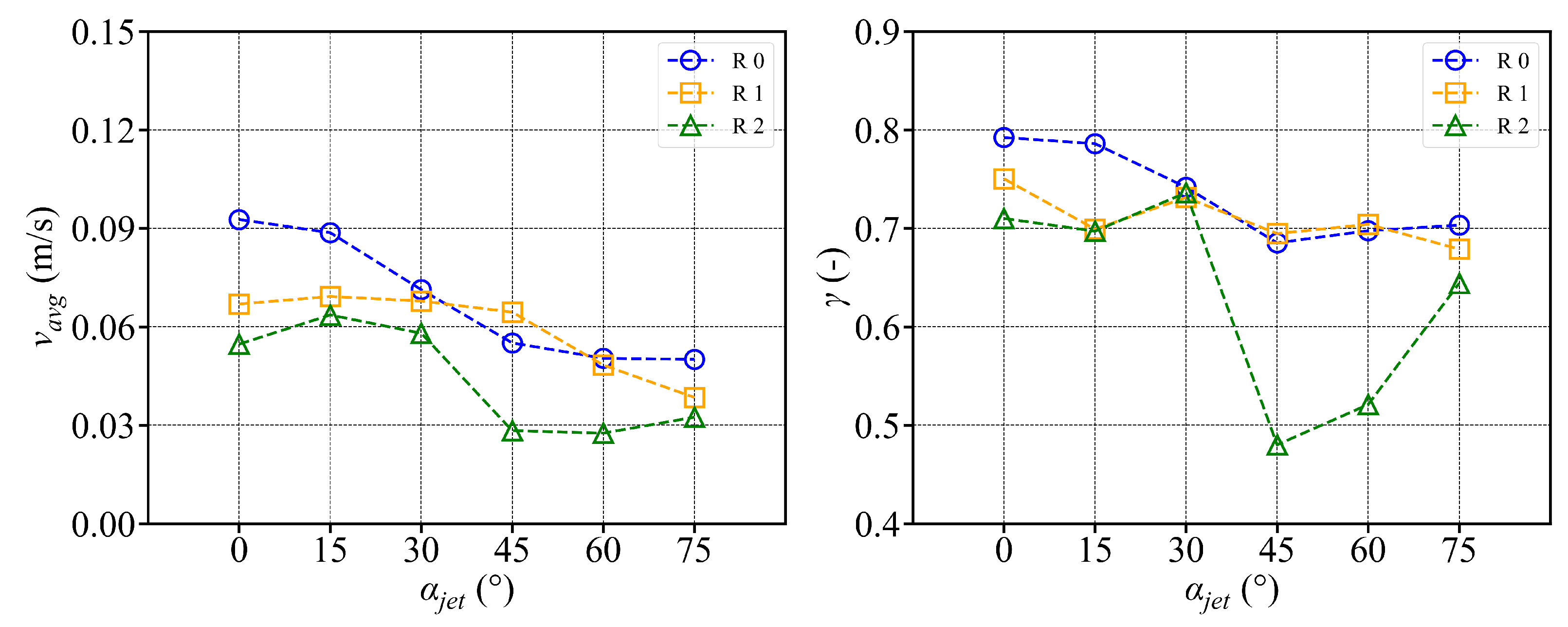
• Compared with arc-shaped tanks, octagonal aquaculture tanks exhibit higher average flow velocities at jet angles of 30° and 45°, while arc-shaped tanks show peak flow velocities at 0° and 15°. In the arc-shaped tanks, the $\gamma$-value is most stable at 0° and decreases with increasing jet angle. This value is also generally higher under low-jet-velocity conditions. In arc-shaped tanks, retaining deflectors results in higher overall flow velocities, particularly at low jet angles. Removing both deflectors leads to increased turbulence, especially under high-jet-angle conditions. At low jet angles (0°–30°), the mean flow velocity decreases as more deflectors are removed. At high jet angles, removing a single deflector has minimal effect on both the mean flow velocity and the flow field trend. In the case of circular boundaries, Scheme A proves to be more effective. Conversely, removing both deflectors substantially increases flow field turbulence.
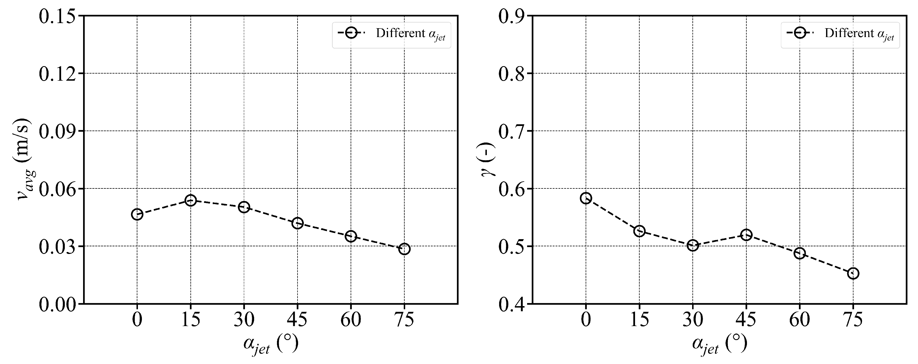
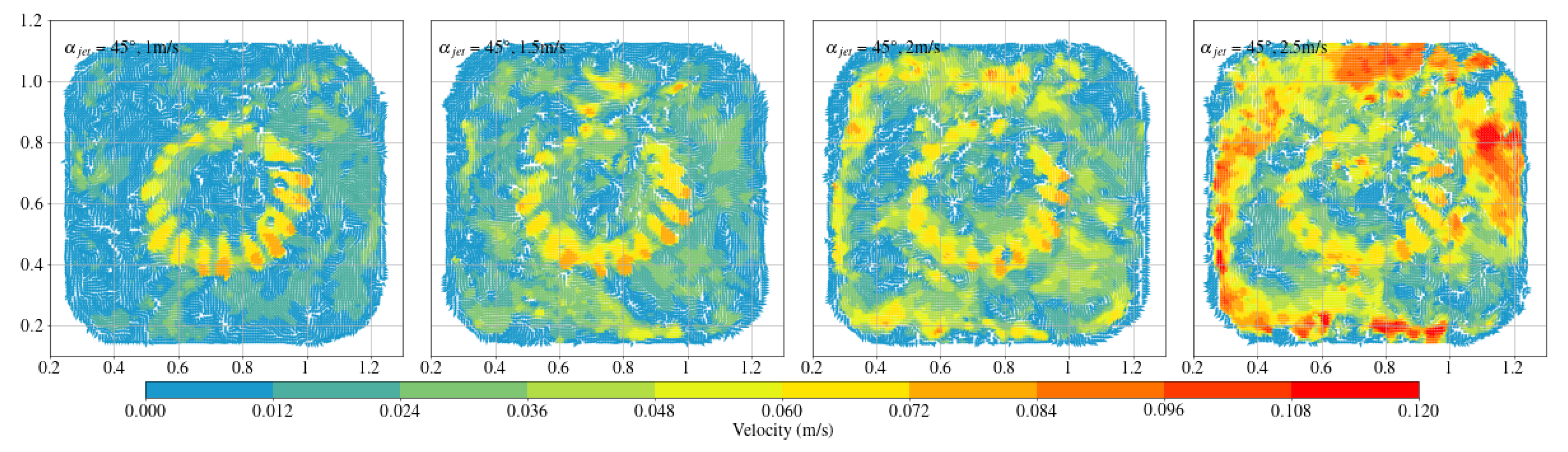
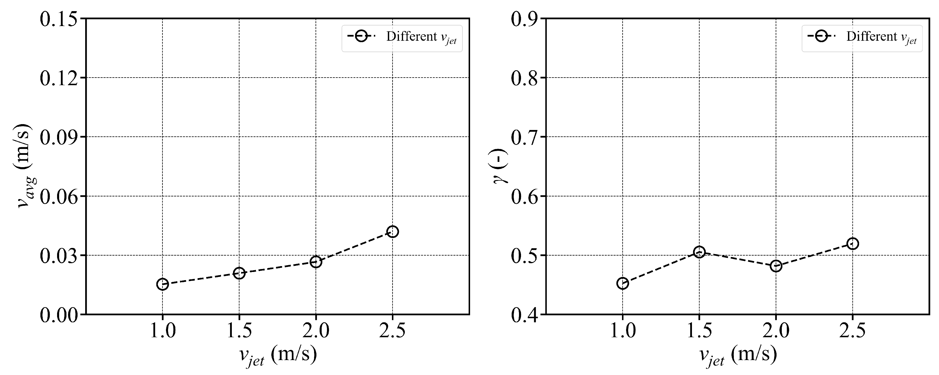
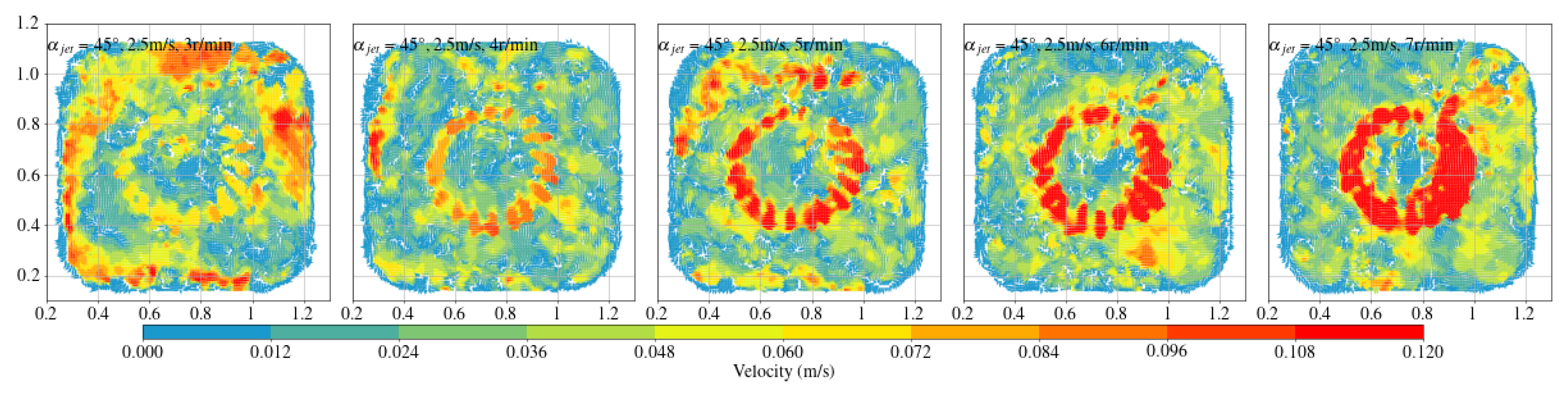
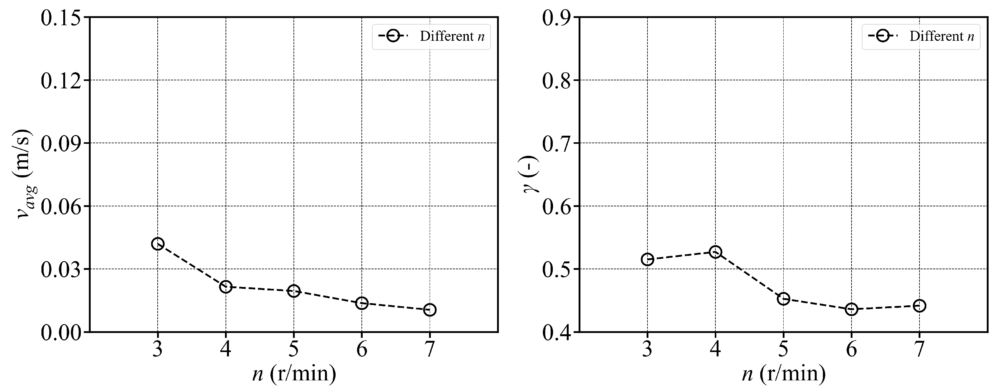
• The fish simulation, experiments were conducted at a jet velocity of 2.5 m/s and a fish rotation speed of 3 rpm under various jet angles, and the trend of mean flow velocity was found to be consistent with that observed in the airspace, peaking at 15°. However, the peak value was 66.875% lower than that in the airspace. Moreover, the overall trend index was 37.5% lower than that in the airspace. These results indicate that fish populations significantly hinder fluid flow and disrupt the stability of the flow field. Under varying jet velocities, the mean flow velocity increased with jet speed, but was reduced by 71.1% at 2.5 m/s compared to that in the airspace. Although the trend index increased overall, it exhibited an average decrease of 34.7% across the four jet velocities. This further confirms that fish disturb the flow field pattern and reduce the mean flow velocity. Disc rotational speeds ranging from 3 rpm to 7 rpm were used to simulate the circular swimming behavior of fish. After removing the high-velocity region near the circular tubes, the overall high-speed region in the flow field was significantly reduced. As the rotational speed increased, flow field disturbance intensified, and the average flow velocity approached zero, while the trend index decreased, indicating that the flow field gradually reached a near-stationary state.
• In aquaculture, when using octagonal tanks and operating under high-jet-velocity conditions, a smaller jet angle (0°–45°) should be selected, and deflector baffles should be retained to maintain a stable flow field, which supports the survival and growth of fish. For arc-shaped tanks, deflectors should be retained at low jet angles (0°–30°) to sustain higher average flow velocities. At higher jet angles, retaining deflectors can help reduce flow field disturbances. This approach helps suppress turbulence in the flow field. In fish farming, jet velocity should be adjusted based on species-specific swimming capabilities to avoid excessive resistance to fish movement.
• This study has certain limitations. The potential influences of fish body size and swimming speed were not fully accounted for in the analysis. Fish of varying body sizes require different spatial allowances within culture tanks; larger fish may demand broader flow field zones to accommodate their swimming behavior, while smaller fish may exhibit different adaptability to flow velocity and field dynamics. Additionally, fish with different inherent swimming speeds may respond differently to variations in jet speed and angle, with fast-swimming species requiring higher flow velocities to mimic natural swimming environments, whereas slow-swimming species may be better suited to lower-velocity conditions.

References

1. Nyström, M.; Jouffray, J.B.; Norström, A.V.; Crona, B.; Jørgensen, P.S.; Carpenter, S.R.; Bodin, Ö.; Galaz, V.; Folke, C. Anatomy and resilience of the global production ecosystem. Nature 2019, 575, 98–108. [Google Scholar] [CrossRef] [PubMed]
2. Xu, H.; Chen, J.; Fang, H.; Zhuang, Z.; Liu, H.; Liu, Y.; Xu, Y. Transformation of China’s Marine Fisheries and Strategic Emerging Industry of Deep Blue Fisheries. Fish. Mod. 2020, 47, 1–9. [Google Scholar]
3. Masaló, I.; Oca, J. Hydrodynamics in a multivortex aquaculture tank: Effect of baffles and water inlet characteristics. Aquac. Eng. 2014, 58, 69–76. [Google Scholar] [CrossRef]
4. Gorle, J.; Terjesen, B.F.; Summerfelt, S.T. Hydrodynamics of octagonal culture tanks with Cornell-type dual-drain system. Comput. Electron. Agric. 2018, 151, 354–364. [Google Scholar] [CrossRef]
5. Davidson, J.; Summerfelt, S. Solids flushing, mixing, and water velocity profiles within large (10 and 150 m3) circular ‘Cornell-type’ dual-drain tanks. Aquac. Eng. 2004, 32, 245–271. [Google Scholar] [CrossRef]
6. Gorle, J.M.; Terjesen, B.F.; Holan, A.B.; Berge, A.; Summerfelt, S.T. Qualifying the design of a floating closed-containment fish farm using computational fluid dynamics. Biosyst. Eng. 2018, 175, 63–81. [Google Scholar] [CrossRef]
7. Nilsen, A.; Hagen, Ø.; Johnsen, C.A.; Prytz, H.; Zhou, B.; Nielsen, K.V.; Bjørnevik, M. The importance of exercise: Increased water velocity improves growth of Atlantic salmon in closed cages. Aquaculture 2019, 501, 537–546. [Google Scholar] [CrossRef]
8. Nilsen, A.; Nielsen, K.V.; Bergheim, A. A closer look at closed cages: Growth and mortality rates during production of post-smolt Atlantic salmon in marine closed confinement systems. Aquac. Eng. 2020, 91, 102124. [Google Scholar] [CrossRef]
9. Tao, Y.; Zhu, R.; Gu, J.; Li, Z.; Zhang, Z.; Xu, X. Experimental and numerical investigation of the hydrodynamic response of an aquaculture vessel. Ocean Eng. 2023, 279, 114505. [Google Scholar] [CrossRef]
10. Xue, B.; Zhao, Y.; Liu, Y.; Cheng, Y. Flow characteristics of an aquaculture vessel with perforated sideboards at various incidence angles. Biosyst. Eng. 2023, 234, 108–124. [Google Scholar] [CrossRef]
11. Oca, J.; Masaló, I. Design criteria for rotating flow cells in rectangular aquaculture tanks. Aquac. Eng. 2007, 36, 36–44. [Google Scholar] [CrossRef]
12. Gorle, J.; Terjesen, B.; Summerfelt, S.T. Hydrodynamics of Atlantic salmon culture tank: Effect of inlet nozzle angle on the velocity field. Comput. Electron. Agric. 2019, 158, 79–91. [Google Scholar] [CrossRef]
13. Xue, B.; Zhao, Y.; Bi, C.; Cheng, Y.; Ren, X.; Liu, Y. Investigation of flow field and pollutant particle distribution in the aquaculture tank for fish farming based on computational fluid dynamics. Comput. Electron. Agric. 2022, 200, 107243. [Google Scholar] [CrossRef]
14. Wang, D. Experimental Study on the Effects on Fish of Flow Turbulent; Hohai University: Nanjing, China, 2007; pp. 42–50. (In Chinese) [Google Scholar]
15. Song, B.; Lin, X.; Wang, W.; Li, G. Effects of water velocities on rheotaxis behaviour and oxygen consumption rate of tinfoil barbs Barbodes schwanenfeldi. Acta Zool. Sin. 2008, 54, 686–694. [Google Scholar] [CrossRef]
16. Tang, M.F.; Xu, T.J.; Dong, G.H.; Zhao, Y.P.; Guo, W.J. Numerical simulation of the effects of fish behavior on flow dynamics around net cage. Appl. Ocean. Res. 2017, 64, 258–280. [Google Scholar] [CrossRef]
17. Che, Z.; Ren, X.; Zhang, Q. Research progress on hydrodynamics in a recirculating aquaculture tank system: A review. J. Dalian Ocean Univ. 2021, 36, 886–898. [Google Scholar] [CrossRef]
18. Plew, D.R.; Klebert, P.; Rosten, T.W.; Aspaas, S.; Birkevold, J. Changes to flow and turbulence caused by different concentrations of fish in a circular tank. J. Hydraul. Res. 2015, 53, 364–383. [Google Scholar] [CrossRef]
19. Masaló, I.; Oca, J. Influence of fish swimming on the flow pattern of circular tanks. Aquac. Eng. 2016, 74, 84–95. [Google Scholar] [CrossRef]
20. An, C.H.; Sin, M.G.; Kim, M.J.; Jong, I.B.; Song, G.J.; Choe, C. Effect of bottom drain positions on circular tank hydraulics: CFD simulations. Aquac. Eng. 2018, 83, 138–150. [Google Scholar] [CrossRef]
21. Liu, N.; Liu, S.; Yu, G. Numerical simulation of and research on hydrodynamic characteristics of two dual-channel circular aquaculture ponds. Fish. Mod. 2017, 44, 1–6. [Google Scholar]
22. Liu, H.; Ren, X.; Zhang, Q.; Bi, C. Numerical modeling of fish movement in a recirculating aquaculture tank: In the case of Schlegel’s black rockfish Sebastes schlegelii. J. Dalian Ocean. Univ. 2021, 36, 995–1002. [Google Scholar] [CrossRef]
23. Yu, L.P.; Xue, B.R.; Ren, X.; Liu, Y.; Xu, T.J.; Shi, X.Y.; Hu, Y.X.; Zhang, Q. Influence of single inlet pipe structure on hydrodynamic characteristics in single-drain rectangular aquaculture tank with arc angles. J. Dalian Ocean. Univ. 2020, 35, 134–140. [Google Scholar] [CrossRef]
24. Shi, X.Y.; Li, M.; Ren, X.Z.; Feng, D.J.; Liu, H.F.; Zhou, Y.X.; Liu, H.B.; Zhao, C.X. Influence of length width ratio on sewage discharge characteristics in acircular rectangular angle culture tank with double inlet pipe structure. J. Dalian Ocean. Univ. 2023, 38, 707–716. [Google Scholar] [CrossRef]
25. Park, S.-G.; Zhou, J.; Dong, S.; Li, Q.; Yoshida, T.; Kitazawa, D. Characteristics of the flow field inside and around a square fish cage considering the circular swimming pattern of a farmed fish school: Laboratory experiments and field observations. Ocean Eng. 2022, 261, 112097. [Google Scholar] [CrossRef]
Figure 1. Experimental setup.
Jmse 13 01023 g001
Figure 2. Tank setup.
Jmse 13 01023 g002
Figure 3. A scheme of the layout and setup of the aquaculture tank.
Jmse 13 01023 g003
Figure 4. Three shapes of aquaculture tanks with octagonal shaped aquaculture tanks as reference.
Jmse 13 01023 g004
Figure 5. Three shapes of aquaculture tanks with circular shaped aquaculture tanks as reference.
Jmse 13 01023 g005
Figure 6. Results of capturing and automatic processing of flow field.
Jmse 13 01023 g006
Figure 7. The results of the average velocity of the flow field for 5 s sampled from the octagonal culture module at rest.
Jmse 13 01023 g007
Figure 8. Maximum difference and standard deviation for different jet angles sampled for 5 s.
Jmse 13 01023 g008
Figure 9. Experiments (left) and the occurrence of vortex phenomena in the “Guoxin 1” aquaculture vessel (right).
Jmse 13 01023 g009
Figure 10. A plot of the flow field (left) as well as a plot of the 50 flow coils (right).
Jmse 13 01023 g010
Figure 11. Results of 30 groups of experimental conditions.
Jmse 13 01023 g011
Figure 12. Flow field results for different jet angles.
Jmse 13 01023 g012
Figure 13. Flow field results for octagonal aquaculture tanks.
Jmse 13 01023 g013
Figure 14. Flow field results after removing one baffle.
Jmse 13 01023 g014
Figure 15. Flow field results after removing two baffles.
Jmse 13 01023 g015
Figure 16. Comparison of results of three shapes at different angles with jet velocity of 2 m/s.
Jmse 13 01023 g016
Figure 17. Results of 30 sets of experimental conditions for circular arc-shaped aquaculture tanks.
Jmse 13 01023 g017
Figure 18. Velocity field results for circular aquaculture tanks.
Jmse 13 01023 g018
Figure 19. Velocity field results after removing one baffle.
Jmse 13 01023 g019
Figure 20. Velocity field results after removing two baffles.
Jmse 13 01023 g020
Figure 21. Mean flow velocity and flow field trend of a circular-shaped culture tank without removing the deflector baffle, with one deflector baffle removed, and with two deflector baffles removed.
Jmse 13 01023 g021
Figure 22. Circumferential swimming of fish in a fish-farming vessel (left) and a device to simulate the movement of fish (right).
Jmse 13 01023 g022
Figure 23. Fish school swimming in a circular pattern (left) and the fish simulator used in the experiment (right).
Jmse 13 01023 g023
Figure 24. Comparison of different jet angles for fish simulation.
Jmse 13 01023 g024
Figure 25. Mean flow velocity and trend index results for different jet angles for fish simulation.
Jmse 13 01023 g025
Figure 26. Comparison of different jet velocities for fish simulation.
Jmse 13 01023 g026
Figure 27. Mean flow velocity and trend index results for different jet velocities in fish simulation.
Jmse 13 01023 g027
Figure 28. Comparison of different rotational speeds for fish simulation.
Jmse 13 01023 g028
Figure 29. Mean flow rate and trend index results at different rotational speeds for fish simulation.
Jmse 13 01023 g029