1. Introduction
The Bragg resonance phenomenon was initially discovered in 1915 by William Henry Bragg and William Lawrence Bragg in X-ray experiments on crystals. They found that wave reflection can be most significant when the crystal spacing is an integer multiple of the half-wavelength of the incident wave [
1]. Later, Miles [
2] proposed a theoretical method for describing the reflection of water waves by small-amplitude undulating sand bars using the boundary integral equation; Davies [
3] further discovered that when water waves propagate over periodic sandbars on the seafloor, Bragg resonance can also occur when the bar spacing is equal to the half of the wavelength. Davies and Heathershaw [
4] conducted experiments to verify the existence of Bragg resonance of water waves. Following these, Mei et al. [
5] proposed the idea of Bragg resonance breakwaters using a set of small-scale, low-elevation artificial parallel bars on the seabed to attenuate waves. Then, considering the cost and environmental benefits of submerged breakwaters, many researchers have studied the Bragg resonance characteristics of various multiple submerged breakwaters through theoretical analysis and numerical simulations. For example, Kirby and Anton [
6] used dominant Fourier mode to analyze the Bragg resonance for sine–cosine sand bars. Cho et al. [
7] used the eigenfunction expansion method to analyze the Bragg resonance for triangular, rectangular, trapezoidal, and semi-circular underwater structures. Liu et al. [
8] presented the analytical solutions of Bragg resonance for triangular, trapezoidal, and cosine sand bars under long-wave conditions based on the modified mild slope equation and determined the optimal configurations of the three shapes. Zeng et al. [
9] studied the Bragg reflection of linear long waves by rectangular sand bars on an inclined seabed, derived a closed analytical solution, and used the analytical solution to obtain the optimal configuration for different numbers of sand waves. Gao et al. [
10,
11] studied the effects of Bragg reflection by submerged sinusoidal bars on harbor resonance. Liu et al. [
12,
13] studied the Bragg reflection by submerged sinusoidal over the reef flat under regular and irregular waves. These studies contributed to the practical use of multiple submerged breakwaters for effective wave attenuation.
Besides submerged breakwaters, floating breakwaters are also characterized by their construction economy and environmental friendliness. Compared to traditional fixed stone or concrete breakwaters, the wave attenuation performance of floating breakwaters may be limited in very high waves, strong currents, or severe storms. The maintenance requirements of floating breakwaters are also higher since the floating body, mooring system, and connecting parts may deteriorate due to exposure to the marine environment. However, floating breakwaters have much lower construction costs and better flexibility. They require fewer materials and less intensive foundation work, especially in deep water or areas with soft seabed, and move with the water surface, maintaining their wave-reducing effectiveness in different water-level conditions. Therefore, floating breakwaters are still popular in many scenarios, such as ports and harbor protection, marine resorts, aquaculture farms, offshore energy facilities, and emergent protection. Given its simple structure, so far, the pontoon type has been thoroughly studied and widely used against wave attacks. Since the interactions between fluid and floating breakwaters are complex, sophisticated computational fluid dynamics (CFD) models are the effective tools to study the hydrodynamic performance of floating breakwaters. Based on CFD models, the effects of the length, cross-section shape, immersion depth, mooring line system on the wave attenuation performance of pontoon-type floating breakwaters have been well studied [
14,
15,
16]. Although the pontoon-type floating breakwater is convenient to use, the attenuation performance of a single floating box is relatively unsatisfactory. Therefore, some researchers [
17,
18,
19] have also proposed two-pontoon floating breakwaters whose two pontoons are usually connected rigidly. Compared to single pontoons, two-pontoon floating breakwaters have better wave attenuation performance, especially for waves with large amplitudes and long periods. However, this type of floating breakwater poses new requirements for the strength and durability of the connection part between the two pontoons, increasing both the construction cost and difficulty.
Another natural way to increase the floating breakwater number is to just put multiple breakwaters that are not connected rigidly, in which case the mooring system of each pontoon is independent. In this way, the merits of a single pontoon, such as convenient construction and low cost, can be preserved. Moreover, the spacing between the pontoons can be adjusted freely, making it easier to achieve the Bragg reflection of waves. However, so far, research on the wave attenuation performance of multiple independent floating breakwaters is very limited. Previous studies [
20,
21] have mainly focused on stationary floating breakwaters, in which case mooring systems and the motions of breakwaters have been ignored. Recently, Chen et al. [
22] used a CFD model to study the hydrodynamics of twin independent floating breakwaters. It was found that the transmission coefficient of twin floating breakwaters is less than that of single floating breakwaters and the motions of floating breakwaters can influence the total wave attenuation performance. However, in their research, the phenomenon of Bragg resonance and its influencing factors were not given particular attention. Therefore, this study mainly focused on the Bragg resonance characteristics of multiple floating breakwaters with independent mooring systems. The CFD model OpenFOAM was utilized to simulate the interactions between waves and floating breakwaters. The accuracy of wave generation and floating body motion simulation by the model was validated first using existing experimental data. Based on the validated model, numerical experiments were then conducted to investigate, by checking the reflection coefficients, the Bragg resonance characteristics of floating breakwaters and the influences of critical parameters. Moreover, the dissipation coefficients, transmission coefficients, and vorticity were also checked together for a better understanding of the overall wave attenuation performance of multiple floating breakwaters.
2. Methodology
This study utilized OpenFOAM (v2312), an advanced open-source computational CFD software package, to simulate the interactions between waves and multiple floating breakwaters. It offers a wide range of solvers and libraries that are highly suitable for conducting hydrodynamic analysis of floating breakwaters.
2.1. Fluid Solver
In this study, OverInterDymFoam was selected as the fluid solver, which uses Navier–Stokes equations for incompressible fluids to describe motion of fluids:
where
u is the velocity vector of the fluid,
ρ is the density of the fluid,
is dynamic viscosity, and
is the divergence operator. The continuity equation is written as
The model uses the finite volume method (FVM) to directly solve the governing equations.
The free surface is then captured by the volume-of-fluid (VOF) method. In the fluid solver, two immiscible fluids of gas and liquid are treated as one fluid in the domain and applied one set of governing equations. The phase fraction of each fluid is computed in every single cell to track the motion of different phases. The transport equation of the phase fraction is written as
where
α is the phase fraction. In the present study, area with
α = 1 is considered water and
α = 0 means that a cell is filled with air. When 0 <
α < 1, the cell is a mixture of gas and liquid and contains a free surface.
2.2. Meshing
The dynamicOversetFvMesh of OpenFOAM, which is based on overset mesh technique, was selected as the mesh implementation for the wave flume and floating body. It combines the overset mesh technique with dynamic mesh capabilities, allowing for simulations of complex scenarios where geometries move relative to each other. In the overset mesh system, overlapping meshes are used to discretize the computational domain. Each mesh can be optimized for specific regions, like using a fine mesh around some structures and a coarse one for the rest, which enhances the efficiency and accuracy of simulations. The “dynamic” aspect enables the mesh to adapt to the movement of objects in the flow field over time, which is essential for problems of fluid–structure interactions. Since meshes can move and overlap without excessive stretching, compression, or distortion, simulations involving complex motions of floating breakwaters are achievable.
In the dynamic mesh method, the velocity of the mesh needs to be considered in the continuity equation, which is calculated as
where
is the velocity vector of mesh. In dynamic mesh, the movement of the mesh affects momentum transfer. Therefore, corrections for the mesh velocity need to be considered and the momentum equation is then the following:
2.3. Motion Solver
Moreover, the sixDofRigidBodyMotion library was chosen to calculate rigid body motion in overset meshes. The library is based on dynamic meshes and solves displacements and rotations in an object in three dimensions caused by external forces. It can adjust boundary and dynamic meshes according to an object’s motion response to maintain good mesh quality. In every step, it first calculates the resultant force and moment of the object by
where
F is combined forces,
a is the acceleration vector,
M is the combined moment,
is angular acceleration, and
is inertia. Then, the acceleration and angular acceleration are integrated in each step to obtain a new angular velocity,
and velocity,
, by
where
and
are the angular velocity and velocity of the last step. By multiplying them with the step time interval, displacements and rotations of the object are calculated. Then, boundary and overset meshes move according to the motion of the object for maintaining mesh quality. Since a two-dimensional (2D) flume was used in the present study, the floating box only moved in one plane and rotated around one axis.
2.4. Mooring Model
In this study, the behavior of mooring systems was simulated by the mooring system dynamics model MoorDyn [
23,
24,
25]. MoorDyn was developed based on lumped-mass discretization, which discretizes a mooring line into finite uniform segments and assigns the half-weight of two neighboring segments to nodes between them. Factors including axial stiffness, damping forces, weight, and hydrodynamic forces are calculated on nodes. The buoyant force
W of each segment,
, is
where
d is the diameter,
l is the unstretched length,
is the density of the mooring line,
is the density of water, and
g is gravity. The tension
T in cable segment is calculated by
where
E is Young’s modulus and
r is the global position vector of each node. The internal damping force
C for numerical stability is written as
where
is initial damping coefficient, and
is strain rate of the segment.
During the calculation, the motion solver calls on MoorDyn as a restraint and transfers the position and velocity information of the moving body to MoorDyn. Subsequently, MoorDyn can deal with the mooring system, updating the positions and tension of lines and returning the restraining forces and moments to the motion solver. Then, the motion solver can further update the acceleration and angular acceleration of the moving body accordingly. The frequency of information exchange between the motion solver and MoorDyn is determined by the time step set by the users.
4. Results and Discussion
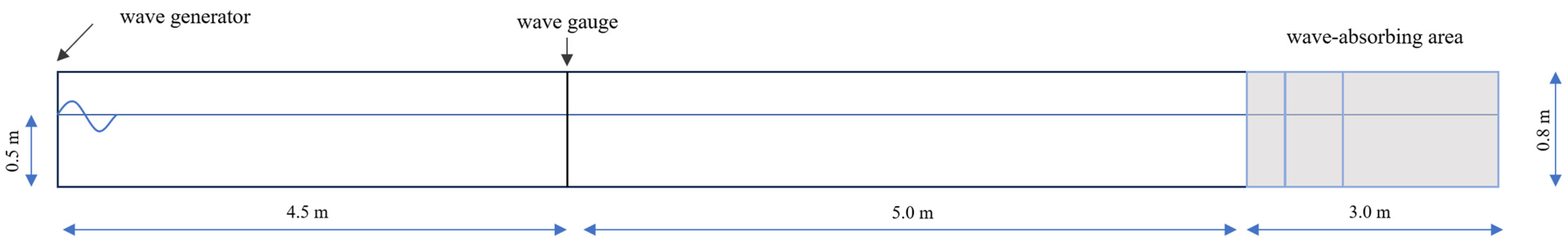
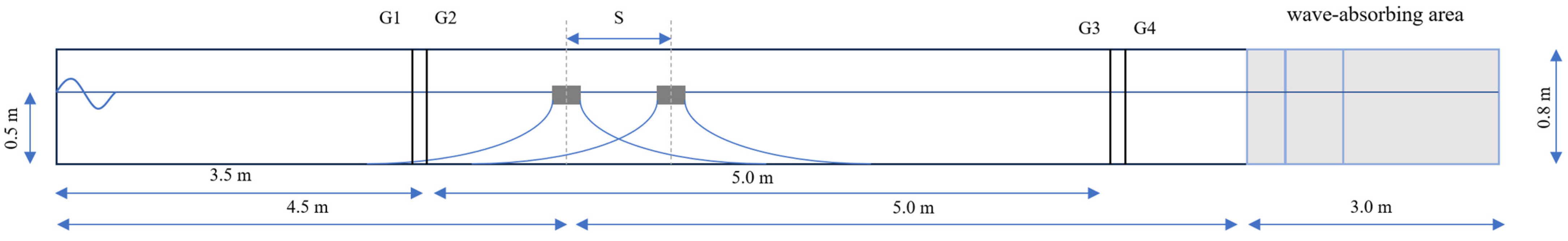
After the validation of the present model, several numerical experiments were conducted to investigate the Bragg resonance and wave attenuation performance of multiple floating breakwaters. The basic numerical setup of this section is shown in
Figure 7. The sizes of the wave flume and the still water depth were the same as the ones detailed in
Section 3. Moreover, multiple floating boxes with independent mooring systems were placed in the flume. The mooring system of each box was the same as the one described in
Section 3. The mass center of the first box was 4.5 m away from the wave generator. Two measurement points (G1, G2) were arranged in front of the floating boxes to calculate the reflection coefficient. Similarly, two measurement points (G3, G4) were arranged behind floating boxes to calculate the transmission coefficient. The distance between the two measurement points was 0.1 m.
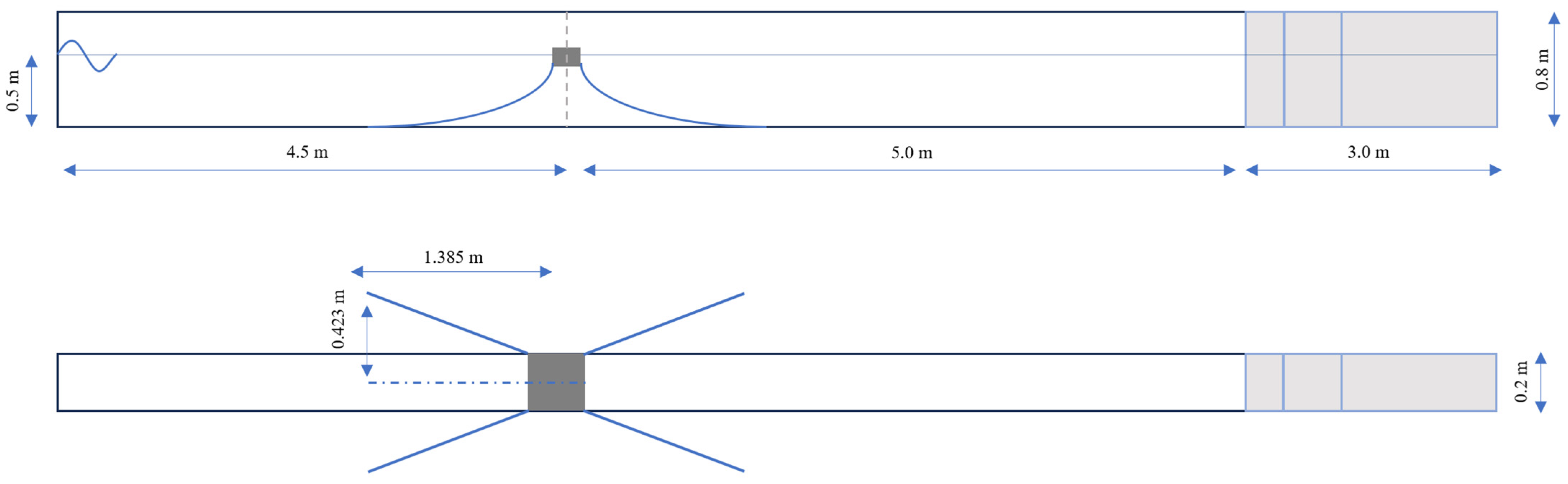
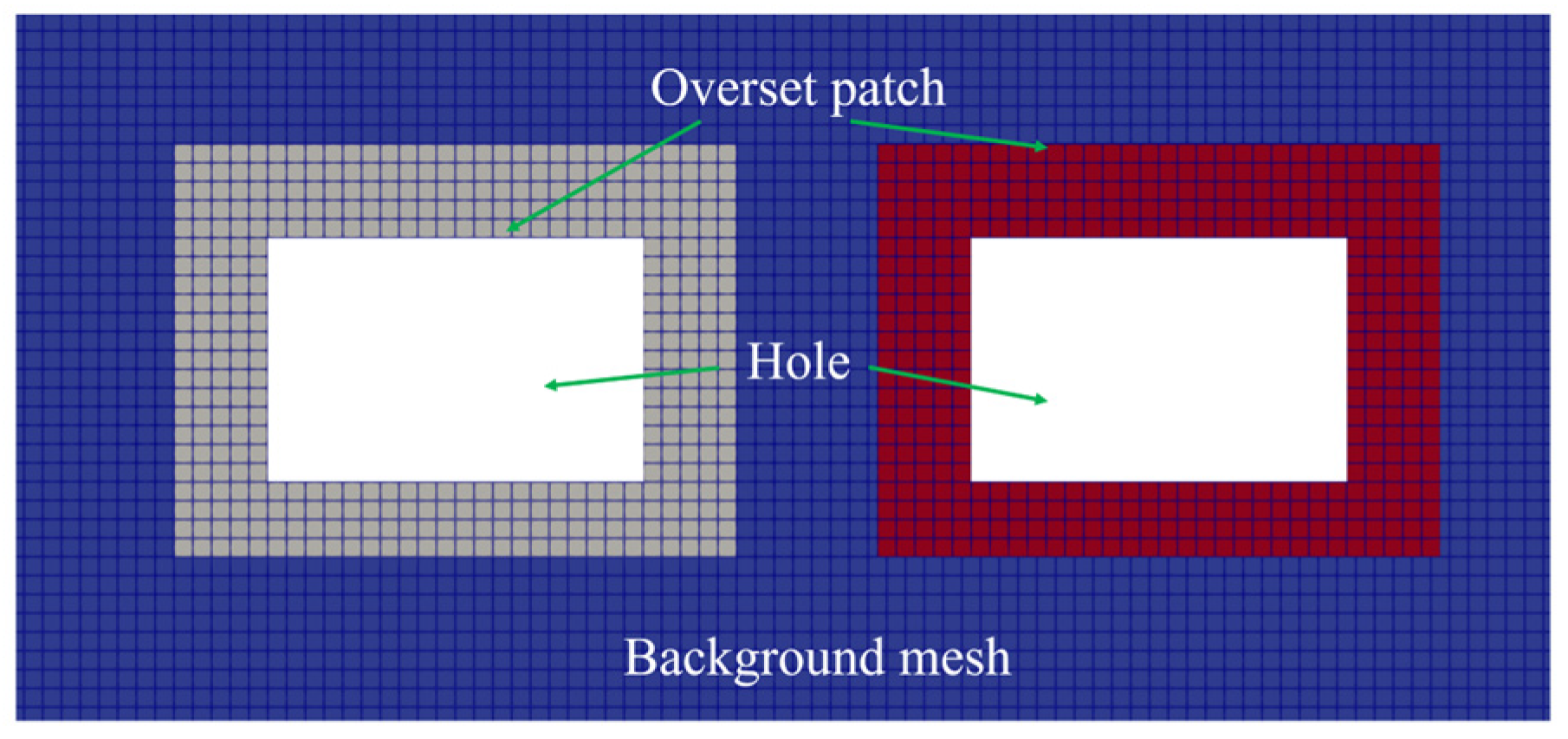
Figure 8 shows the mesh setup for the present numerical experiments. As seen in
Figure 8, three types of meshes were generated: the background mesh, the overset mesh, and the hole cell. The hole cells were used to describe the space occupied by the two floating bodies. The background meshes were used to solve the Navier–Stokes equations for fluids. The overset meshes moved with the floating body and were responsible for performing interpolation on variables in overlapping regions, ensuring the consistency and continuity of the flow field during the mesh movement. The sizes of both overset and background meshes were set as 0.01 m in the horizontal and vertical directions. The time steps of all numerical experiments were set as 0.001 s, in which case the frequency of information exchange between the motion solver and MoorDyn was 1000 Hz.
The conditions of the numerical experiments are listed in
Table 1. Four groups were designed, and Group 1 mainly investigated the Bragg resonance and total wave attenuation performance of twin independent floating boxes when the ratio of the box spacing and half-wavelength 2
S/
L varied (2
S/
L was changed by changing
S). Groups 2 to 4 further investigated the effects of box submergence percentage, length, and quantity on the Bragg resonance and total wave attenuation performance. The size of the floating box in Group 1, 2, and 4 was the same as the one detailed in
Section 3 while the length of the floating box in Group 3 varied from 0.2 m to 0.3 m. The submergence percentage of the floating box was varied by changing the weight of the box. The incident waves for all groups were set as fifth-order Stokes waves with
Hi = 0.06 m and
Ti = 1.0 s (wavelength of
Li = 1.5 m) for the better observation of Bragg resonance.
4.1. Bragg Resonance and Wave Attenuation of Twin Floating Boxes
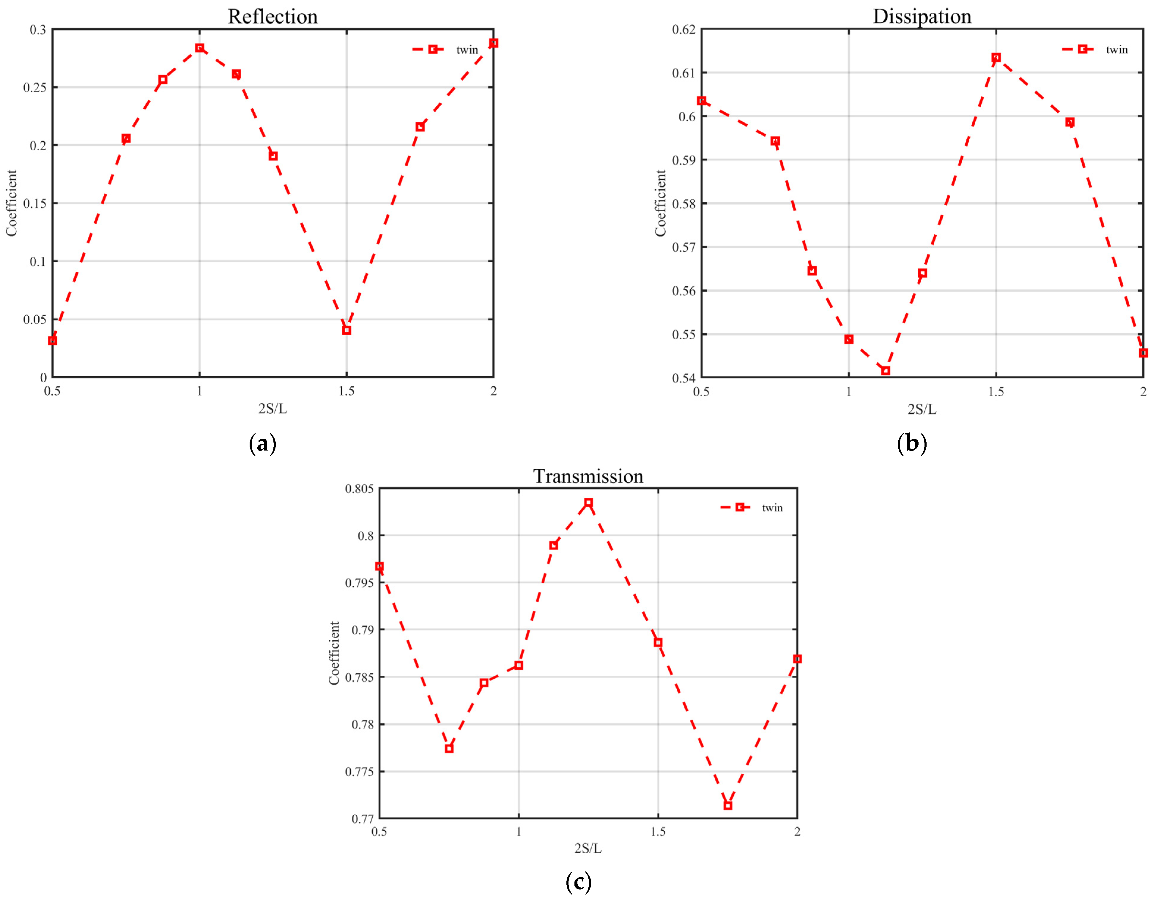
Figure 9 shows the reflection, dissipation, and transmission coefficients of twin independent floating boxes as 2
S/
L varied for Group 1. The specific calculated values can be found in
Table 2. The reflection coefficients
Kr and transmission coefficients
Kt were calculated using Goda’s two-points method [
27]. The dissipation coefficient
Kd was then calculated based on the energy conservation principle:
As seen in
Figure 9a, the reflection coefficient of the twin floating boxes responded to the change in 2
S/
L and local maximum reflection coefficients were observed when 2
S/
L = 1 and 2. This confirms the Bragg reflection effect induced by the twin floating breakwaters. However, the dissipation coefficients of twin floating boxes when 2
S/
L = 1 and 2 were not the largest (
Figure 9b). Instead, local maximum dissipation coefficients were observed when 2
S/
L = 0.5 and 1.5. For floating breakwaters, wave energy is typically dissipated through turbulence generated by the motion of floating breakwaters [
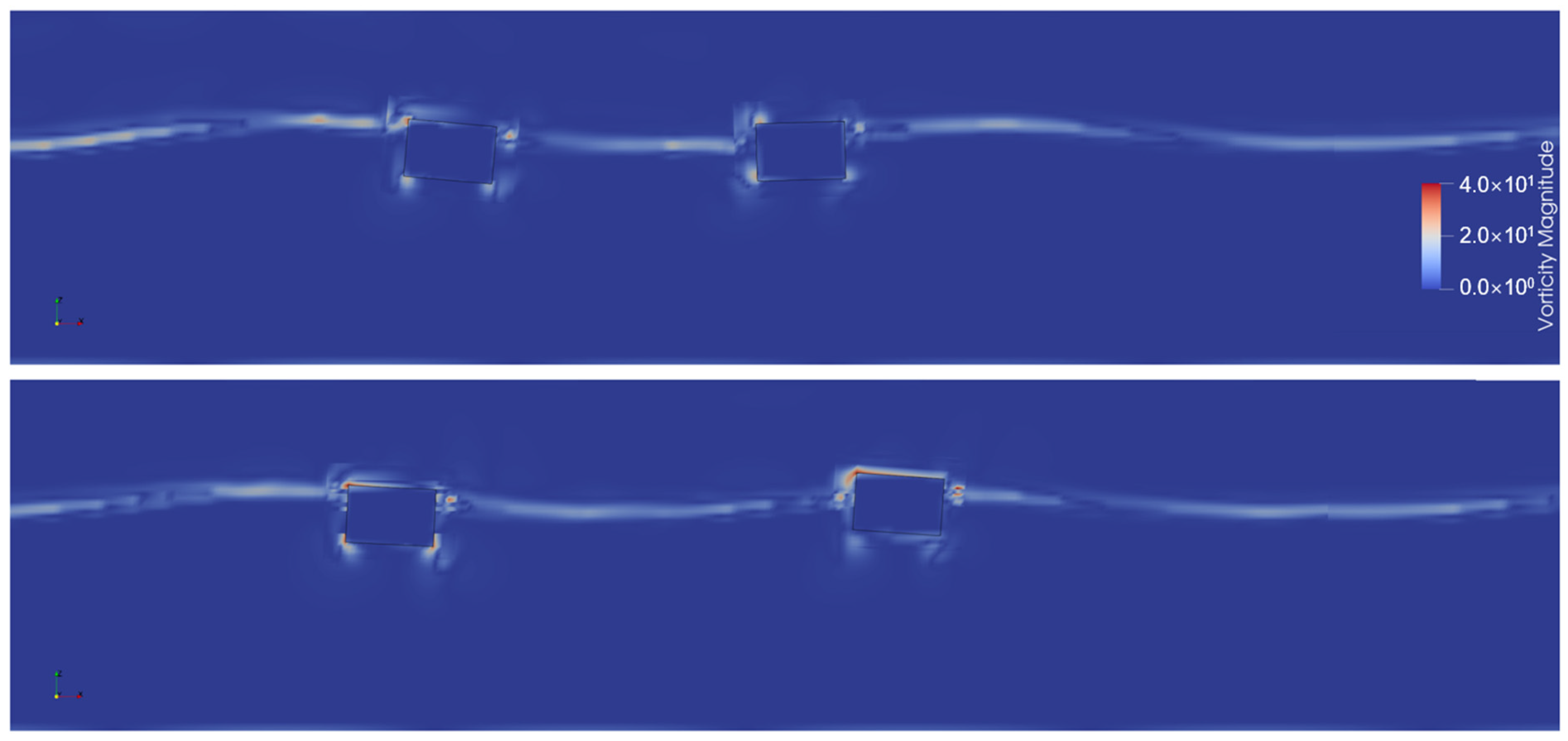
22]. Therefore, we further checked the vorticity near the floating breakwater when 2
S/
L = 1 and 1.5 (
Figure 10). Stronger vorticity was produced around both two boxes with 2
S/
L = 1.5, especially around the top corners of two boxes and the submerged corners of the first box, confirming that the twin floating boxes with 2
S/
L = 1.5 induced more wave dissipation. Due to the combined effects of reflection and dissipation, the lowest transmission coefficients were observed at 2
S/
L = 0.75 and 1.75 where both the reflection and dissipation were relatively large.
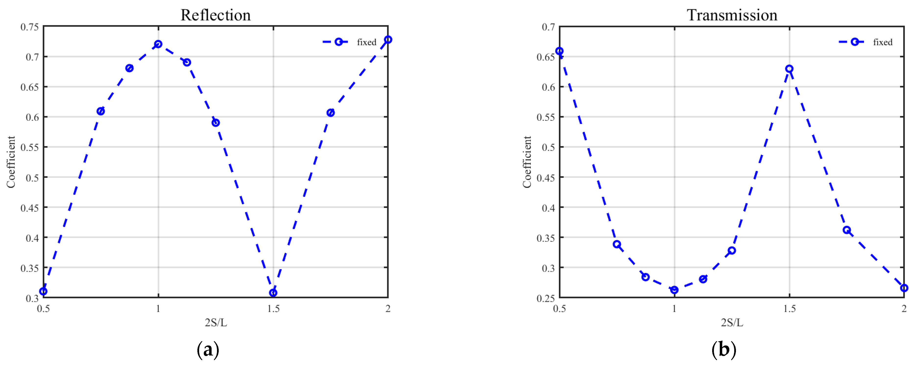
Figure 11 shows the reflection and transmission coefficients as 2
S/
L varied when both floating boxes were fixed. When the twin floating boxes were fixed, local maximum reflection coefficients were still observed at 2
S/
L = 1 and 2 but the reflection effect was much greater than that of the moving floating boxes. The trend of variation in the transmission coefficient was obviously dominated by the reflection effect and exhibited local minimum values at 2
S/
L = 1 and 2. This reveals that the optimal conditions for wave attenuation by moving floating bodies differ from those of stationary ones. Also, we have to mention that although the fixed floating boxes exhibited much stronger reflection and lower transmission, it is difficult to implement completely fixed floating boxes in reality.
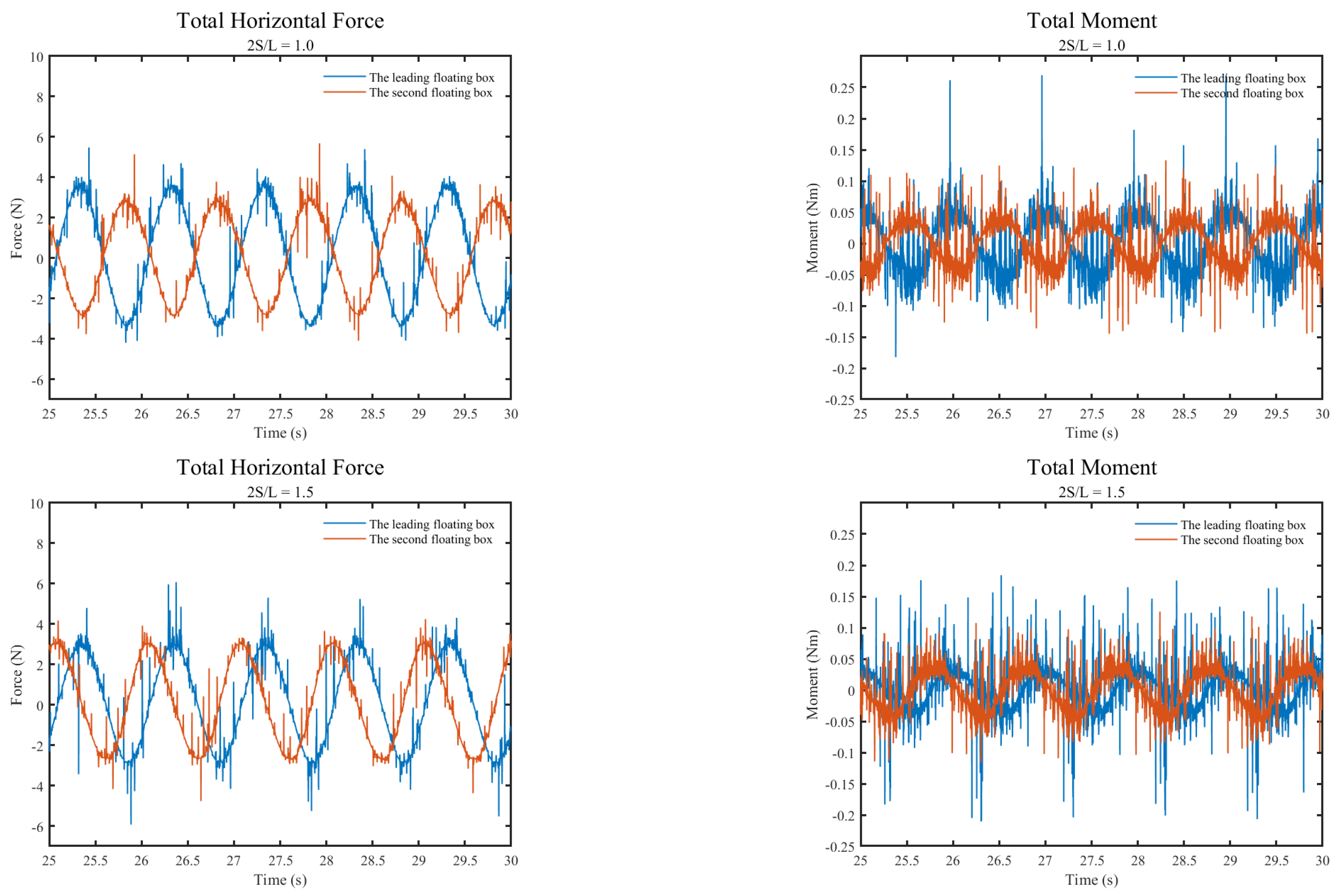
Figure 12 further shows the time-varying total horizontal forces and total moments of the two floating boxes when 2
S/
L = 1 and 1.5. When 2
S/
L = 1, the peaks of the horizontal total force for the first floating box were a little higher, and the valleys were a little lower than those for the second floating box. When 2
S/
L = 1.5, the peaks and valleys of the horizontal total force for the two floating boxes were similar in magnitude. The curves of the total horizontal force and moment exhibited an overall trend of change caused by wave actions, but there were also many small fluctuations, presumably due to turbulence around the boxes. Moreover, when 2
S/
L = 1, the overall trends of the horizontal total force variations, as well as the moment variations, for the first and second floating boxes were exactly in opposite phases. This further indicates that the two floating boxes should have been in a state of Bragg resonance when 2
S/
L = 1.
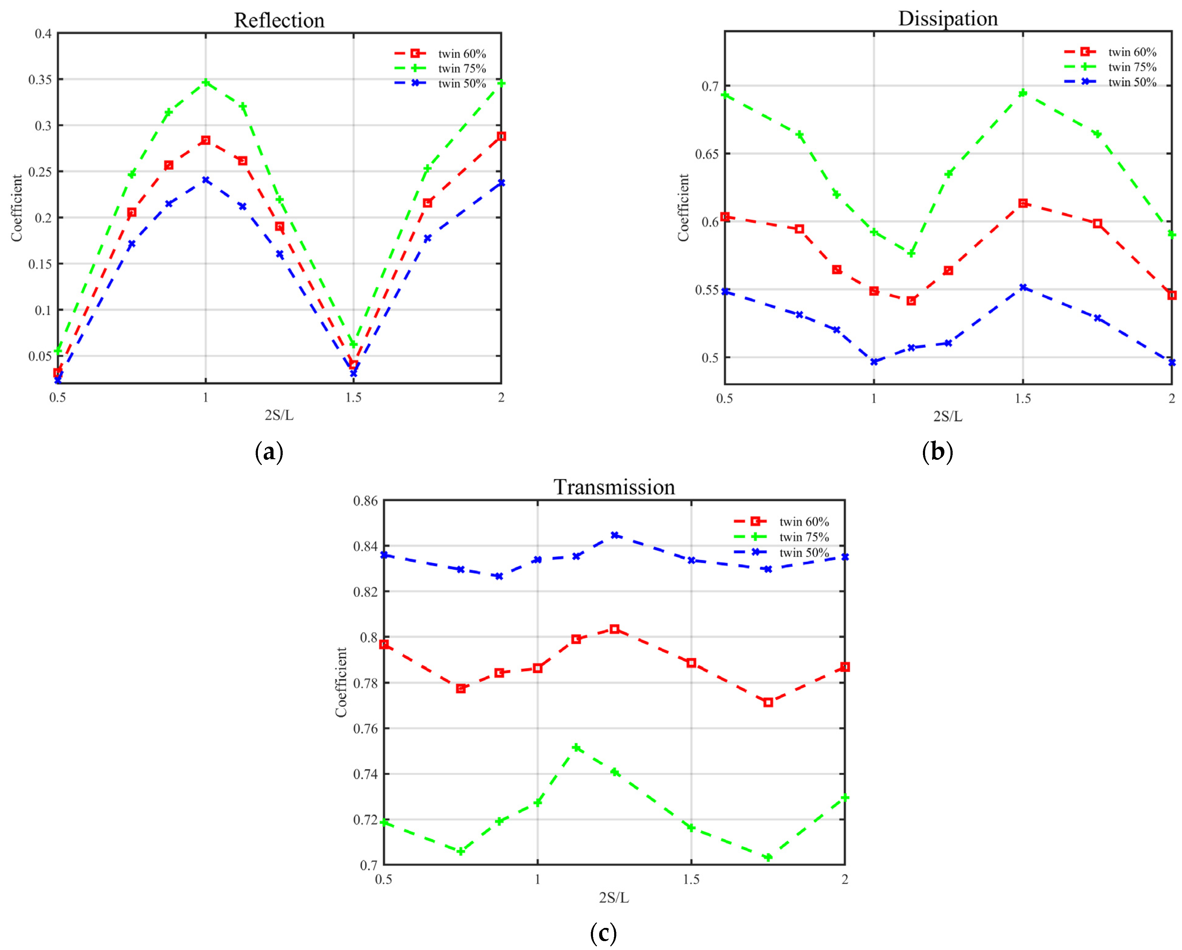
4.2. Effect of Submergence Percentage
Figure 13 shows the reflection, dissipation, and transmission coefficients of twin independent floating boxes as 2
S/
L varied with different submergence percentages for Group 2. The specific calculated values can be found in
Table 3 and
Table 4. As seen in
Figure 13, the variation trends of all coefficients as 2
S/
L varied did not change for different submergence percentages. As the submergence percentage increased, the reflection and dissipation coefficients increased and the transmission coefficient decreased. The reflection coefficient increased by 44% as the submergence percentage rose from 50% to 75% at 2
S/
L = 1.0. At 2
S/
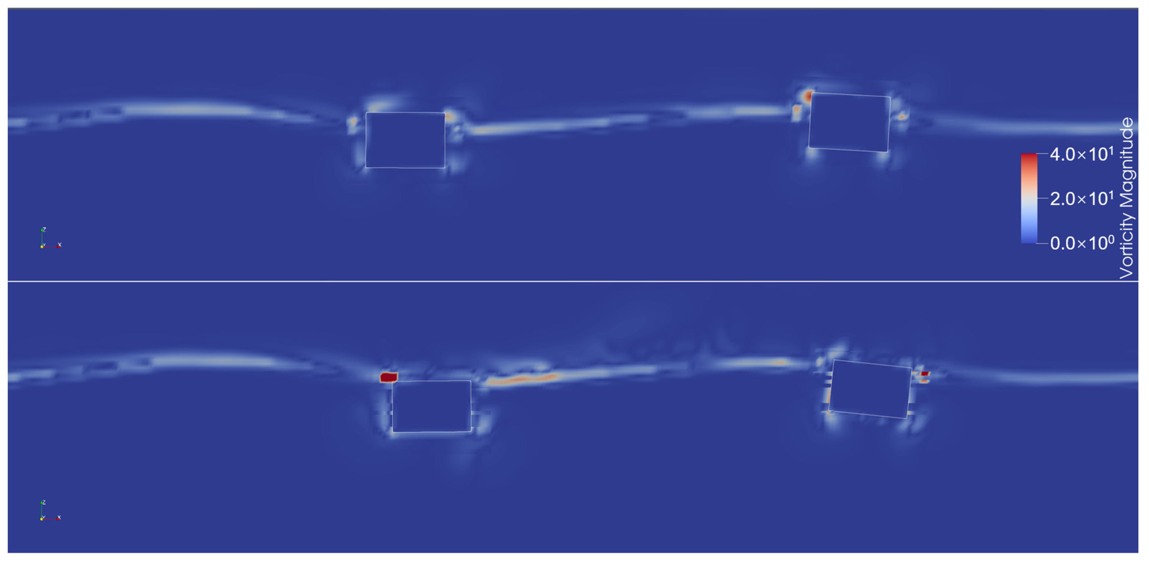
L = 1.75, the transmission coefficient decreased by 17%. Regarding the effect of submergence on reflection, it is easily understood that a larger immersion depth resulted in a higher reflection coefficient. Regarding the effect of submergence percentage on dissipation,
Figure 14 further shows the distribution of vorticity near the twin floating breakwaters at 2
S/
L = 1.5 when the submergence percentage was 50% and 75%. It can clearly be seen that floating boxes with deeper immersion depth showed stronger vorticity, especially around the top corners of the two floating boxes. The vorticity around the submerged corners of the two boxes with deeper immersion depth was also stronger.
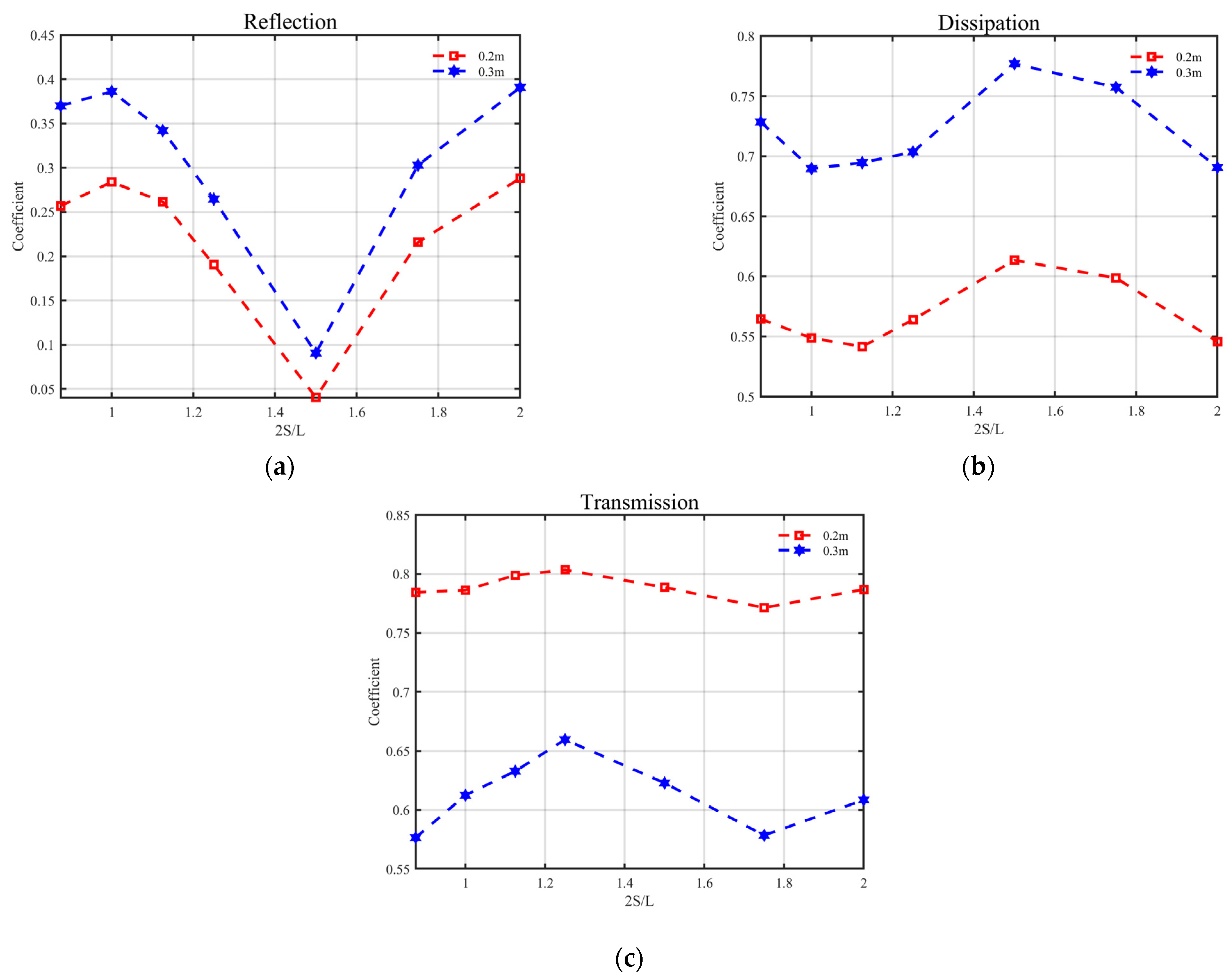
4.3. Effect of Length of Floating Breakwaters
Figure 15 shows the reflection, dissipation, and transmission coefficients of twin independent floating boxes as 2
S/
L varied with different lengths of floating boxes for Group 3. The specific calculated values can be found in
Table 5. Like those in Group 2, the variation trends of all coefficients as 2
S/
L varied did not change for different lengths. The reflection and dissipation coefficients increased and the transmission coefficient decreased as the length increased from 0.2 m to 0.3 m. The reflection coefficient increased by 36% while the dissipation coefficient increased by 26% at 2
S/
L = 1.0.
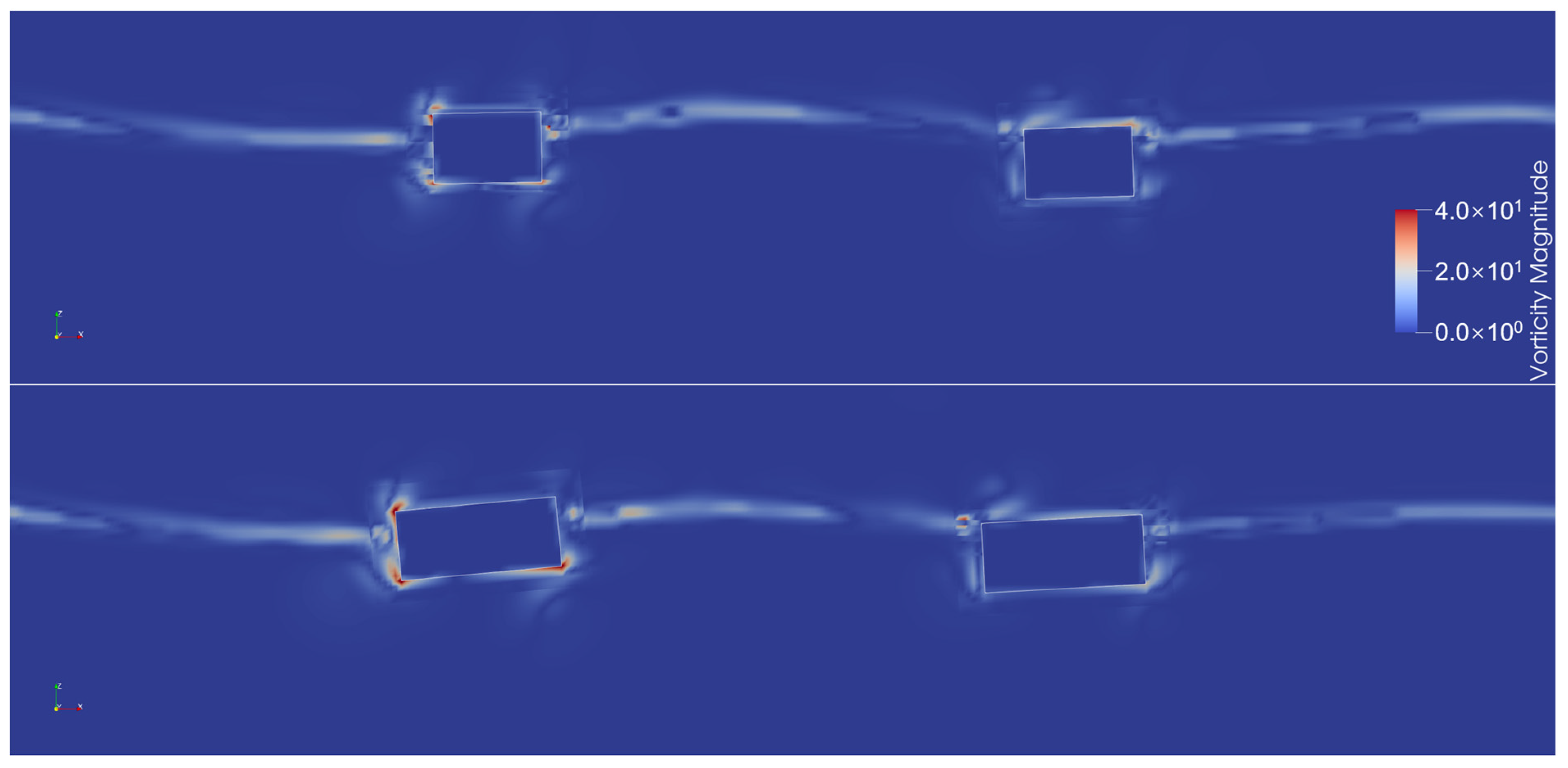
Figure 16 further shows the distribution of vorticity near twin floating breakwaters at 2
S/
L = 1.5 when the box length was 0.2 m and 0.3 m. Longer twin floating boxes induced stronger vorticity, especially around top and submerged corners of the leading floating box.
4.4. Effect of Quantity of Floating Breakwaters
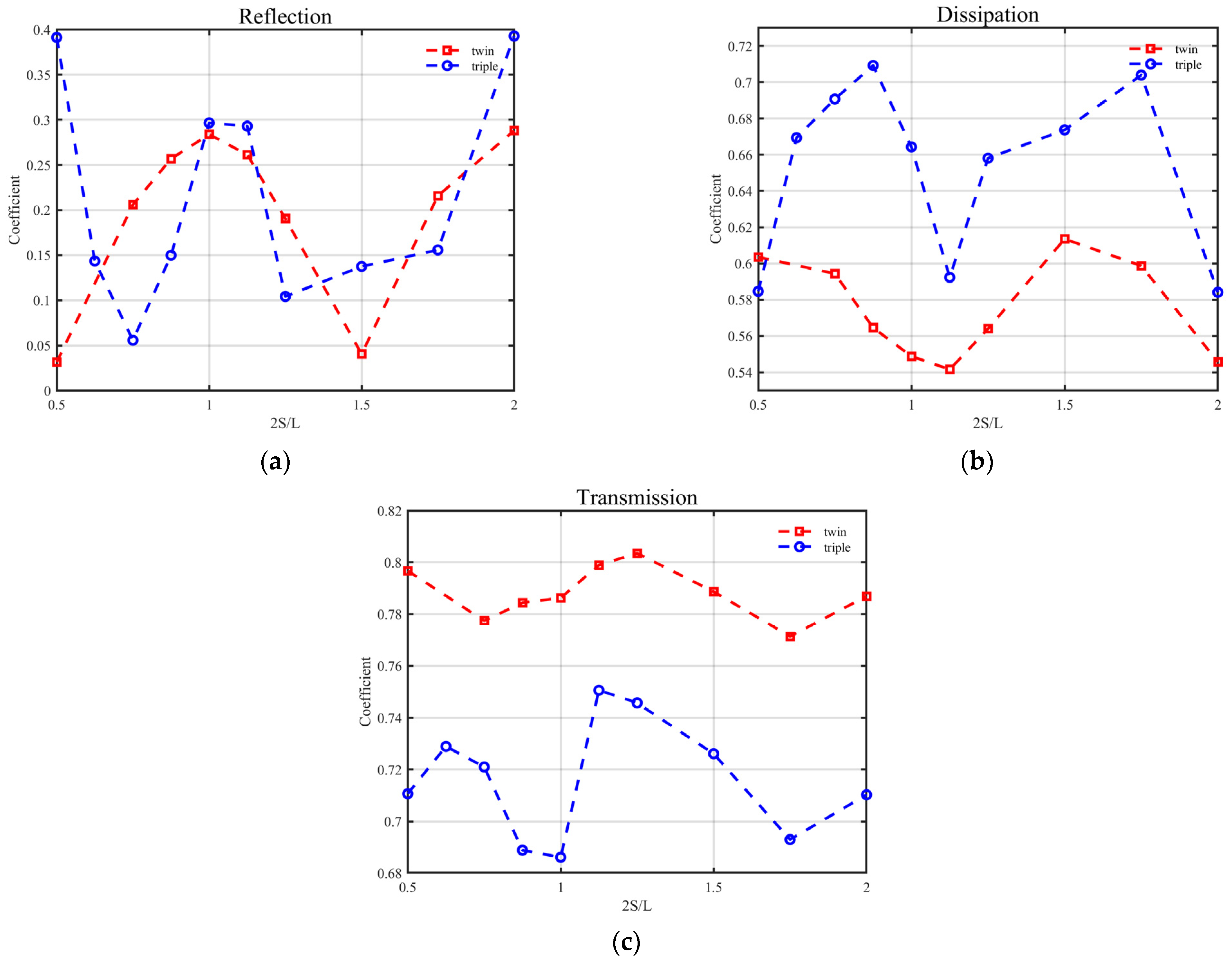
Figure 17 shows the reflection, dissipation, and transmission coefficients as 2
S/
L varied with different quantities of floating breakwaters for Group 4. The specific calculated values can be found in
Table 6. As seen in
Figure 17, overall, with an increase in the number of pontoons to three, the variation in wave reflection was insignificant, while wave energy dissipation was obviously enhanced, thereby reducing the wave transmission coefficient.
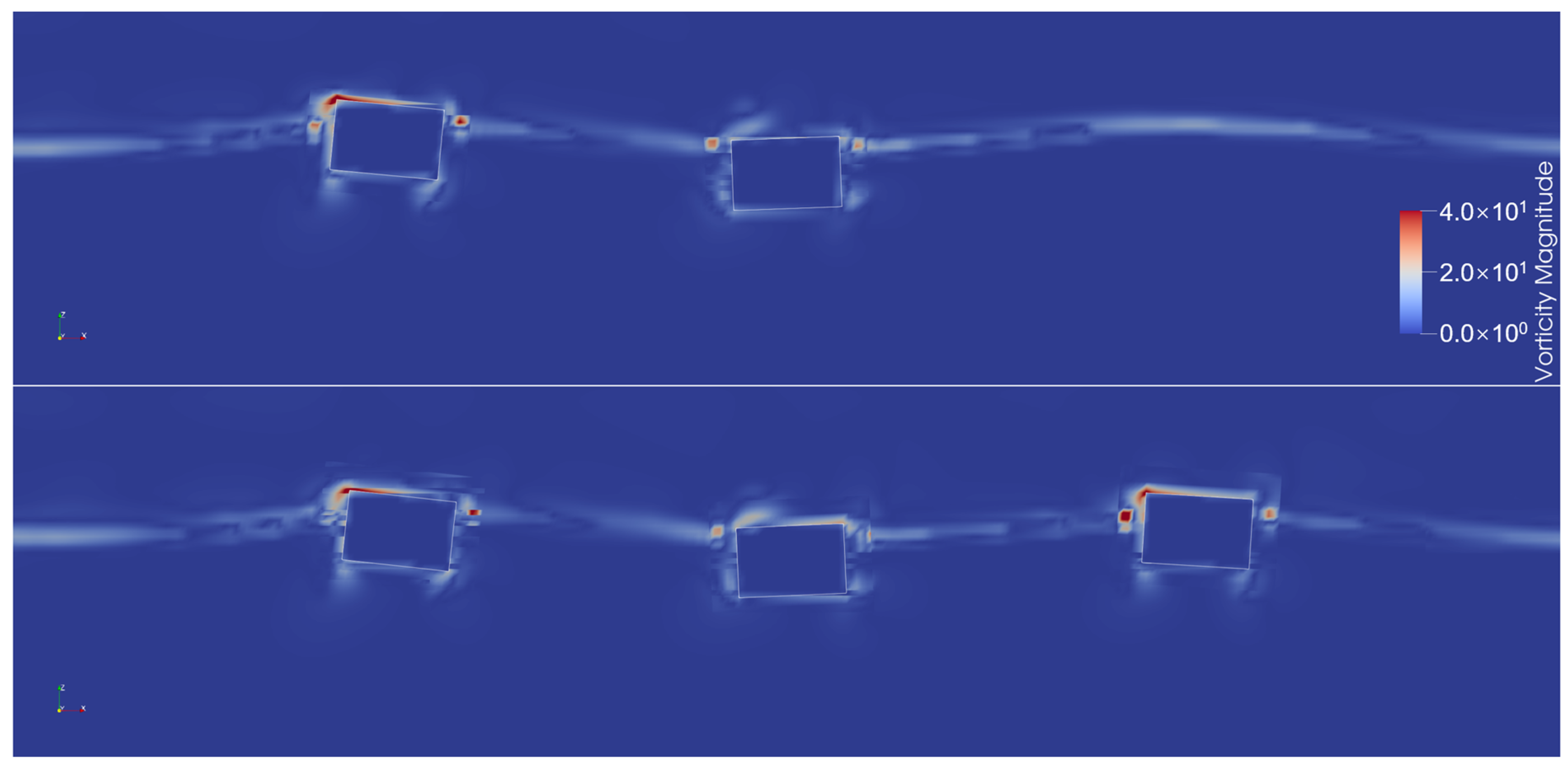
Figure 18 further shows the vorticity near floating breakwaters at 2
S/L = 1 with box quantities of two and three. The increase in dissipation as the box quantity grew was mainly induced by the additional box. Moreover, the variation trends of all coefficients as 2
S/
L varied of the three floating breakwaters were different from the ones of the two floating breakwaters. The difference mainly occurred when 2
S/
L < 1.25. As seen in
Figure 17a, the reflection coefficient of three floating breakwaters still exhibited extrema at the positions of 2
S/
L = 1 and 2
S/
L = 2, indicating the presence of Bragg reflection phenomenon. However, when 2
S/
L was less than 0.75, the reflection coefficient showed an increasing trend, and the reflection coefficient at 2
S/
L = 0.5 was even higher than that at 2
S/
L = 1. This should be because when the spacings of the three pontoons were small, their reflection effect more closely resembled that of a single long pontoon, thereby enhancing the reflection effect. As seen in
Figure 17b, when the spacings of the three pontoons were small, the wave energy dissipation effect of three pontoons was instead reduced. This may be because when the three pontoons were closely spaced and resembled a single long pontoon, their motions became constrained, thereby reducing the wave energy dissipation.
5. Conclusions
This study utilized a computational fluid dynamics (CFD) model to analyze the Bragg resonance characteristics of multiple independently moored floating breakwaters and the influences of critical parameters. The associated energy dissipation, wave transmission, and vorticity near the breakwaters were also checked to better understand the overall wave attenuation performance of multiple floating breakwaters. The main conclusions are drawn as follows:
- (1)
Bragg resonance can be induced by multiple floating breakwaters. However, the condition corresponding to the maximum Bragg resonance reflection does not coincide with that of the maximum wave energy reduction. For twin floating breakwaters, the value of 2S/L at the optimal wave attenuation tends to be smaller than that at the Bragg resonance.
- (2)
Increasing the immersion depth and length of the floating breakwater can enhance both the effects of Bragg reflection and wave energy dissipation, thereby improving the overall wave attenuation performance of multiple floating breakwaters. A deeper immersion depth mainly intensifies vorticity around the top corners of floating boxes, while a longer box length predominantly enhances vorticity around the leading box.
- (3)
Increasing the number of floating boxes has a relatively small impact on the Bragg reflection effect, but it enhances the wave energy dissipation of the floating boxes, thereby improving the overall wave attenuation performance. The increase in dissipation as box quantity grows is mainly induced by the additional box.
We acknowledge that the conclusions are only derived based on the conditions set in this study, which only considered regular waves and a two-dimensional flow field. However, in reality, wave conditions are irregular and vary with location, and the flow field is also three dimensional. Additionally, the mooring system may also influence the Bragg reflection and wave energy dissipation effect of multiple floating breakwaters. Therefore, future research can be explored in these areas.


