Exploring Dissipation Terms in the SPH Momentum Equation for Wave Breaking on a Vertical Pile

Abstract

Accurate simulation of fluid flow around vertical cylinders is essential in numerous engineering applications, particularly in the design and assessment of offshore structures, bridge piers, and coastal defenses. This study employs the smoothed particle hydrodynamics (SPH) method to investigate the complex dynamics of breaking waves impacting a vertical pile, a scenario marked by strong free-surface deformation, turbulence, and the wave–structure interaction. The mesh-free nature of SPH makes it especially suitable for capturing such highly nonlinear and transient hydrodynamic phenomena. The primary objective of the research is to evaluate the performance of different SPH dissipation schemes, namely artificial viscosity, laminar viscosity, and sub-particle scale (SPS) turbulence models, in reproducing key hydrodynamic features. Numerical results obtained with each scheme are systematically compared against experimental data to assess their relative accuracy and physical fidelity. Specifically, the laminar + SPS model reproduced the peak horizontal wave force within 5% of experimental values, while the artificial viscosity model overestimated the force by up to 25%. The predicted wave impact occurred at a non-dimensional time of $t/T\approx 0.28$, closely matching the experimental observation. Furthermore, force and elevation predictions with the laminar + SPS model remained consistent across three particle spacings ($dp=0.05\mathrm{m},0.065\mathrm{m},0.076\mathrm{m}$), demonstrating good numerical convergence. This work provides critical insights into the suitability of SPH for modeling wave–structure interactions under breaking wave conditions and highlights the importance of proper dissipation modeling in achieving realistic simulations. The performance of the dissipation schemes remained robust across three tested particle spacings, confirming consistency in force and elevation predictions. Additionally, it underscores the sensitivity of SPH predictions to spatial resolution, highlighting the need for careful calibration to ensure robust and reliable outcomes. The study contributes to advancing SPH as a practical tool for engineering design and hazard assessment in coastal and offshore environments.

1. Introduction

Vertical piles are essential structural components in offshore wind turbines, bridge piers, mooring systems, and berthing facilities [1,2,3,4]. Their interaction with water waves involves complex hydrodynamic phenomena, such as vortex shedding, pressure fluctuations, and wave breaking, all of which contribute to the force exerted by water on these structures [5,6,7]. The extensive use of vertical piles in marine environments underscores the vital importance of advancing numerical techniques to improve the structural stability and long-term performance of vertical piles, thanks to better modeling of the wave–structure interaction. Offshore wind turbines (OWT), for example, are complex structural–mechanical systems deployed in harsh marine environments, where they are subjected to highly variable wind, wave, and current loads [8]. Their design requires a multidisciplinary approach that addresses dynamic interactions among turbine components and environmental forces, soil–structure interaction, and long-term fatigue behavior. A system-based, performance-oriented design philosophy is essential, supported by multi-scale modeling and uncertainty quantification to ensure reliability and cost-efficiency. In particular, wave-induced loading is a critical factor in OWT support structure design. Hydrodynamic forces, comprising drag and inertia components, can dominate shear and bending responses depending on wave height and wind speed combinations. Design analyses must therefore evaluate multiple load cases: proper characterization of these load effects is vital to ensure structural integrity and optimal turbine performance. Indeed, an accurate prediction of wave-induced forces on all structures in coastal and offshore areas, including those made up of piles, is imperative to properly address the design and fabrication of marine engineering structures.

The increasing frequency of extreme weather events, mainly driven by climate change [9], underscores the need for reliable simulations of severe hydrodynamic conditions, particularly those that involve waves breaking [10]. Although significant advances have been made in modeling the forces exerted by non-breaking waves on piles [11,12,13], the complex dynamics of breaking waves remain an active area of research [14,15,16]. Understanding the interaction of breaking waves with marine structures is essential to improve the predictive capabilities of numerical models and optimize the design of resilient marine infrastructure. As an example, the accurate numerical prediction of wave-induced turbulence and its direct influence on wave-breaking mechanisms remains a challenge. Mesh-based approaches require substantial computational resources to resolve free-surface phenomena accurately, while the use of particle methods often leads to excessive numerical dissipation or inadequate turbulence modeling. Thus, one of the immediate needs is improved numerical formulations capable of reliably capturing complex turbulence dynamics associated with wave breaking on structures.

This study investigates the effectiveness of energy dissipation mechanisms in smoothed particle hydrodynamics (SPH) [17] to enhance the reliability of simulations, with a particular focus on interactions between highly nonlinear waves breaking on a cylindrical vertical pile. Traditional computational approaches, such as the finite-volume and finite-element methods, rely on turbulence models such as Reynolds-averaged Navier–Stokes (RANS) and large eddy simulation (LES) to resolve the dynamics of the wake [18,19]. Although effective in many applications, these methods struggle with highly nonlinear free-surface phenomena, such as breaking waves and violent splashing. SPH offers an alternative approach that discretizes the fluid domain into material particles which obey the Navier–Stokes equations in a Lagrangian framework [20,21,22,23].

Several works have been found in which SPH has been used to model waves breaking on vertical cylinders. In Wen et al. [24], a parallel SPH-LES numerical wave basin was used to study the interaction of waves with coastal structures, including vertical cylinders. They noted a strong agreement between the numerical and experimental data for the free surface elevation, horizontal wave forces, and overturning moments, validating SPH for the analysis of structural wave loading. In Chow et al. [11], a numerical wave basin is presented to model wave interactions with cylindrical vertical structures. Their model was based on incompressible SPH (ISPH) with graphics processing unit (GPU) acceleration, and it simulated focused wave groups hitting a cylinder, providing a comparison of the results with experimental data to analyze the hydrostatic and non-hydrostatic pressures. Yang et al. [14] employed an SPH-based numerical model to predict wave forces on a vertical cylinder in the presence of near-breaking and spilling, breaking waves. The model employs artificial viscosity as a dissipation term to stabilize the simulation [17]. The authors’ work accurately replicated extreme wave conditions, showing good agreement with the experimental data for surface elevation and horizontal forces. In addition, they captured higher forces from spilling breaking waves and the secondary load cycle. Tasora et al. [25] incorporated Project Chrono [26] to model the dynamic response, which improved the predictions of cylinder vibrations and secondary load cycles and confirmed SPH as a reliable tool for offshore structure assessments under extreme wave conditions.

The modeling of turbulence and viscosity with SPH presents several unique numerical challenges arising from its mesh-free nature and discrete particle formulation. The relatively low-order spatial accuracy of SPH discretization, the inherent particle disorder, particularly evident in regions with high vorticity, and the complex fluid–boundary interactions near walls complicate the accurate representation of viscous and turbulent flow dynamics. Several modeling strategies have been developed to address turbulence and viscosity in SPH simulations. Early contributions focused primarily on viscosity through the introduction of artificial viscosity models [17], which improve numerical stability but often introduce excessive numerical diffusion. The laminar viscosity model proposed by [27] provided a physically consistent treatment of viscous forces, although it neglected the sub-particle turbulence effects critical in high-Reynolds-number flows. On the turbulence modeling front, early SPH formulations adopted approaches inspired by traditional turbulence closure models. For instance, adaptations of the Lagrangian averaged Navier–Stokes (LANS) $\alpha$-model [28,29], later reformulated as the $ϵ$-model [30,31,32], were developed to capture unresolved turbulent motions through velocity smoothing across neighboring particles. Further advancements incorporated Reynolds averaged Navier–Stokes (RANS) turbulence closures such as the k-$ϵ$ and explicit algebraic Reynolds stress models (EARSM) into SPH frameworks [33,34], demonstrating promising agreement with experimental data, particularly for free-surface flows and boundary layers [35,36]. More recently, attention has shifted towards large eddy simulation (LES)-based methods due to the inherent similarity between SPH interpolation and LES filtering operations. Pioneering LES-SPH studies by [37,38] demonstrated the potential of LES to model turbulent wave breaking, overtopping, and dam-break scenarios. However, unresolved numerical challenges such as overpredicted velocities due to insufficient vortex resolution [39] highlight ongoing difficulties in achieving accurate LES implementations in SPH. The sub-particle scale (SPS) model [40] has emerged as a compelling approach for explicitly addressing unresolved turbulent motions at the particle scale, but its performance remains insufficiently assessed for breaking wave interactions with vertical structures. For instance, more recently, [41] demonstrated the feasibility of integrating SPH within the framework of large eddy simulations by proposing a quasi-Lagrangian LES-SPH model capable of capturing high-Reynolds-number turbulent flows.

Given the distinct strengths and limitations of these viscosity and turbulence approaches, a systematic and comparative analysis is warranted to evaluate their suitability specifically for wave-induced hydrodynamic loading on vertical structures. Therefore, this study aims to elucidate how various dissipation mechanisms, such as the artificial viscosity, the laminar viscosity, and the SPS turbulence model, affect the accuracy of SPH simulations in capturing wake dynamics, vortex shedding, and resulting structural forces. Through this investigation, the ultimate goal is to improve the predictive accuracy and reliability of SPH in engineering design and hazard assessment applications involving complex wave–structure interactions.

It is important to clarify that, in the context of this study, the structural response of the pile (e.g., deformation or vibration) is not modeled. The vertical cylinder is treated as a fully rigid body. This modeling assumption is well-established in both experimental and numerical modeling applied to coastal engineering (e.g., [42,43,44]), where the focus lies on evaluating hydrodynamic loads exerted by waves on fixed or quasi-fixed structures. Although the term “wave–structure interaction” (WSI) is used throughout the paper, it refers to the hydrodynamic interaction with a non-deforming structure, not to the fully coupled fluid–structure interaction (FSI) problem where both fluid and structural equations are solved simultaneously. The latter approach is more common in aeroelasticity or flexible-structure analyses [45]. We acknowledge that assuming undeformability may be idealized, but it remains a justified approximation for the objective of this work: assessing the accuracy of SPH hydrodynamic force predictions under breaking waves.

Our numerical investigation is based on previous CFD modeling in [15], where a comprehensive analysis is shown for the mesh-based representation of breaking waves on a vertical pile. Their work used experimental data from [46] as a benchmark for validating numerical models, underscoring the importance of a turbulence closure model in accurately predicting wave forces. In the present study, the same experimental test case is employed.

The structure of the article is as follows. Section 1 provides the background and motivation for the work. Section 2 is devoted to a comprehensive description of the SPH method, encompassing its underlying equations and dissipation schemes. Section 3 introduces the experimental setup that was utilized for the validation. Section 4 presents the primary findings on wave profiles and forces. Section 5 examines the velocity fields and turbulence characteristics. Finally, Section 7 draws our conclusion with a summary of the most significant findings.

2. Methodology: Smoothed Particle Hydrodynamics (SPH)

Simulations are carried out using the open-source DualSPHysics solver, fully described in [47], which employs a weakly compressible smoothed particle hydrodynamics (SPH) method [17,48]. DualSPHysics is designed to operate on both CPU and GPU. Usually, viscosity effects in SPH are incorporated into the momentum equation to simulate the resistance of the fluid to deformation and internal friction. Among the commonly used techniques, the artificial viscosity (AV) term [20] has been widely employed to mimic the behavior of real viscosity in fluid dynamics. This term plays a crucial role in smoothing flow discontinuities and mitigating numerical instabilities, particularly in areas with steep velocity gradients or shock waves. The artificial viscosity is typically calibrated based on local velocity gradients, ensuring the desired level of dissipation while minimizing potential disruptions to the overall flow behavior. Its primary purpose is to dissipate kinetic energy and stabilize velocity fluctuations, effectively simulating viscous effects. Beyond the artificial viscosity, the laminar + sub-particle scale (SPS) model is used to treat turbulent flows in situations where direct resolution of fine-scale turbulence is computationally expensive. This approach combines a laminar flow model and a subgrid turbulence model. The laminar model is described in [37], and it simplifies the bulk flow by solving the Navier–Stokes equations without explicitly modeling turbulence. To account for unresolved turbulent structures, the SPS model in [38] can be leveraged to capture the energy dissipation induced by the turbulent eddies at scales smaller than the SPH particle size. Specifically, the Smagorinsky model [49] forms the basis of this formulation, adding a viscosity term to the Navier–Stokes equations to dampen turbulent fluctuations and enhance the accuracy of the simulation.

2.1. Fundamentals of SPH

Smoothed particle hydrodynamics (SPH) is a mesh-free numerical method that represents a continuum as a set of discrete particles. Each particle bears fluid properties (e.g., density, velocity, mass, etc.) and moves in accordance with the governing equations. The behavior of a particle is influenced by its neighboring particles within a predefined interaction radius, determined by the smoothing length (h). The contribution of each neighbor is weighted using a kernel function (W), ensuring a smooth interpolation of fluid properties.

The SPH formulation is based on an integral approximation of any function $F\left(\mathbf{r}\right)$:

$$F\left(\mathbf{r}\right)={\int }_{\mathbf{\Omega }}F\left({\mathbf{r}}^{\prime }\right)W(\mathbf{r}-{\mathbf{r}}^{\prime })d{\mathbf{r}}^{\prime }.$$

(1)

In discrete form, this equation can be approximated as follows:

$$F\left({\mathbf{r}}_a\right)=\sum _{b}F\left({\mathbf{r}}_b\right)W({\mathbf{r}}_a-{\mathbf{r}}_b,h){\displaystyle \frac{m_b}{{\rho }_b}},$$

(2)

where subscripts a and b denote the target and neighboring particles, respectively, m is the particle mass, and $\rho$ is the fluid density; $\mathbf{r}$ denotes the spatial position vector. Different kernel functions are proposed in the literature, two of which are implemented in DualSPHysics, i.e., the cubic and Wendland kernels [47]. In the present study, we employ the Wendland kernel [50], provided by the following:

$$W\left(q\right)={\alpha }_D{\left(1-{\displaystyle \frac{q}{2}}\right)}^4(2q+1),0\le q\le 2,$$

(3)

where $q=r/h$ is the normalized inter-particle distance, and ${\alpha }_D$ is a normalization factor ensuring mass conservation.

2.1.1. SPH Governing Equations

The governing equations for fluid motion in SPH generally include the continuity and Navier–Stokes (momentum) equations, respectively:

$${\displaystyle \frac{d{\rho }_a}{dt}}={\rho }_a\sum _b{\displaystyle \frac{m_b}{{\rho }_b}}{\mathbf{v}}_{ab}·{\nabla }_a{W}_{ab}+D_a,$$

(4)

$${\displaystyle \frac{d{\mathbf{v}}_a}{dt}}=-\sum _b{m}_b\left({\displaystyle \frac{P_a+P_b}{{\rho }_a{\rho }_b}}\right){\nabla }_a{W}_{ab}+{\mathbf{\Gamma }}_a+\mathbf{g},$$

(5)

where $\mathbf{v}$ is the velocity, ${\mathbf{\Gamma }}_a$ is the dissipation term, $\mathbf{g}$ is the gravity acceleration, $\rho$ is the density, and P is pressure. The second term on the right-hand side of Equation (4) corresponds to a density diffusion term [51], $D_a$, which stabilizes fluctuations in the SPH density field, and is defined as follows:

$$D_a=2\delta h{c}_s\sum _b({\rho }_{ba}^T-{\rho }_{ab}^H){\displaystyle \frac{{\mathbf{r}}_{ab}·{\nabla }_a{W}_{ab}}{r_{ab}^2}}{\displaystyle \frac{m_b}{{\rho }_b}},$$

(6)

where $c_s$ is the speed of sound, and $\delta$ is a tuning parameter that controls the magnitude of the diffusion term, typically set at 0.1 [47].

2.1.2. Dissipation and Turbulence Modeling

To account for dissipation effects, the momentum equation includes additional viscosity terms. If an AV model is applied, the dissipation term is written as follows:

$${\displaystyle \frac{d{\mathbf{v}}_a}{dt}}=-\sum _b{m}_b\left({\displaystyle \frac{P_b+P_a}{{\rho }_b·{\rho }_a}}+{\mathrm{\Pi }}_{ab}\right){\nabla }_a{W}_{ab}+\mathbf{g}.$$

(7)

Here,

$${\mathrm{\Pi }}_{ab}=\left\{\begin{array}{cc}{\displaystyle \frac{-\alpha c_{ab}{\mu }_{ab}}{{\rho }_{ab}}}\hfill & {\mathbf{v}}_{ab}·{\mathbf{r}}_{ab}<0\hfill \\ 0\hfill & {\mathbf{v}}_{ab}·{\mathbf{r}}_{ab}\ge 0\hfill \end{array}\right.,$$

(8)

where ${\mathbf{r}}_k$ is the particle position vector. The parameter $c_{ab}$ is the mean speed of sound, ${\rho }_{ab}$ is the mean density, ${\mu }_{ab}=(h{\mathbf{v}}_{ab}·{\mathbf{r}}_{ab})/(|{\mathbf{r}}_{ab}{|}^2+{\eta }^2)$, with ${\eta }^2=0.01h^2$, and $\alpha$ is a coefficient that needs to be tuned to introduce the appropriate amount of dissipation. The value $\alpha =0.01$ has been shown to yield optimal results when validating wave flume experiments involving wave propagation and the resulting wave loads on coastal structures [52]. However, as emphasized by Altomare et al. [53], careful consideration of the value selected for $\alpha$ and the numerical resolution employed becomes particularly important when modeling wave-breaking conditions.

If the laminar + SPS scheme is used, the dissipation term in the momentum equation is replaced with the following:

$${\mathbf{\Gamma }}_a=\sum _b{m}_b{\displaystyle \frac{4{\nu }_0{\mathbf{r}}_{ab}·{\nabla }_a{W}_{ab}}{({\rho }_a+{\rho }_b)(r_{ab}^2+0.01h^2)}}{\mathbf{v}}_{ab}+\sum _b{m}_b\left({\displaystyle \frac{{\tilde{\tau }}_a^{ij}+{\tilde{\tau }}_b^{ij}}{{\rho }_a{\rho }_b}}\right){\nabla }^i{W}_{ab}.$$

(9)

The first term in Equation (9) represents the laminar viscosity, with ${\nu }_0$ being the kinematic viscosity of the fluid, which is equal to $1\times {10}^{-6}{\mathrm{m}}^2/\mathrm{s}$. The second term accounts for the SPS turbulence model [38], which introduces eddy viscosity via the Smagorinsky model:

$${\displaystyle \frac{{\tilde{\tau }}^{ij}}{\rho }}={\nu }_t\left(2{\tilde{S}}^{ij}-{\displaystyle \frac{2}{3}}{\tilde{S}}^{ii}{\delta }^{ij}\right)-{\displaystyle \frac{2}{3}}{C}_L{\Delta }^2{\delta }^{ij}{|{\tilde{S}}^{ij}|}^2.$$

(10)

Here, ${\nu }_t={(C_S\Delta )}^2{|{\tilde{S}}^{ij}|}^2$ is the eddy viscosity, $C_S=0.12$ is the Smagorinsky constant, and $C_L=0.0066$. The symbol $\Delta$ denotes the initial particle spacing.

2.1.3. Equation of State

DualSPHysics employs a weakly compressible SPH (WCSPH) approach, where the pressure is calculated directly from the density field using a stiff equation of state as follows:

$$p={\displaystyle \frac{c_s^2{\rho }_0}{\gamma }}\left[{\left({\displaystyle \frac{\rho }{{\rho }_0}}\right)}^{\gamma }-1\right].$$

(11)

Here, ${\rho }_0$ is the reference density, and $\gamma$ is the polytropic constant, characterized by a high value ($\gamma =7$). To ensure that the density variations remain small, typically within 1% of the reference density, a numerical speed of sound, $c_s$, is chosen such that the Mach number $M=\parallel v_{\max }\parallel /c_s\approx 0.1$, where $v_{\max }=\sqrt{g{h}_0}$ corresponds to the characteristic maximum velocity usually adopted for the dam-break problem, with $h_0$ being the initial height of the fluid in the domain. In this way, the fluid is treated as almost incompressible.

2.2. Boundary Conditions

2.2.1. Modified Dynamic Boundary Conditions

In SPH, specific boundary conditions (BC) are employed to handle interactions between solid bodies and fluid particles. The DualSPHysics solver utilizes dynamic boundary conditions (DBC), which are recognized for their simplicity, robustness, computational efficiency, and relatively accurate treatment of complex geometries [54]. However, DBCs may introduce a non-physical gap between the solid boundary and adjacent fluid particles. To solve this issue, modified boundary conditions (mDBC) were formulated and implemented in [55]. Within this new mDBC framework, boundary particles are positioned analogously to DBC, with the boundary interface located at half a particle spacing inward from the innermost boundary particle layer. For each boundary particle, a ghost node is projected into the fluid region across the interface. The boundary particles receive fluid properties using the values calculated at the ghost node and an extrapolation method highlighted in [56].

2.2.2. Open Boundary Conditions

In DualSPHysics, open boundary conditions are modeled using the methodology in [56], further refined for coastal engineering applications in [57,58,59]. A special buffer region near the domain boundaries is created, where velocity and pressure boundary conditions are prescribed. Fluid particles in these buffer regions ensure proper particle interaction and kernel support. Inlet boundaries typically prescribe velocity conditions for the incoming fluid, while outlets can set pressure or velocity conditions for the exiting fluid.

3. Case Study: Large-Scale Experiments by Irschik et al. [46]

The case study examined in the sources refers primarily to the large-scale model tests conducted by Irschik et al. [46] in the large wave channel (GWK) of the Coastal Research Center in Hannover, Germany. These experiments investigated breaking wave loads on a slender pile in shallow water. The experiments aimed to understand the forces exerted by breaking waves on the pile, noting that these forces are a superposition of a slowly varying force and an additional impulsive force of short duration (i.e., slamming) due to the impact of the breaker front. Furthermore, the experimental study concentrated on determining the curling factor, an empirical coefficient related to the height of the impact area. Data from these large-scale model tests are frequently used to validate CFD simulations of progressive waves breaking on a vertical pile, e.g., in [15].

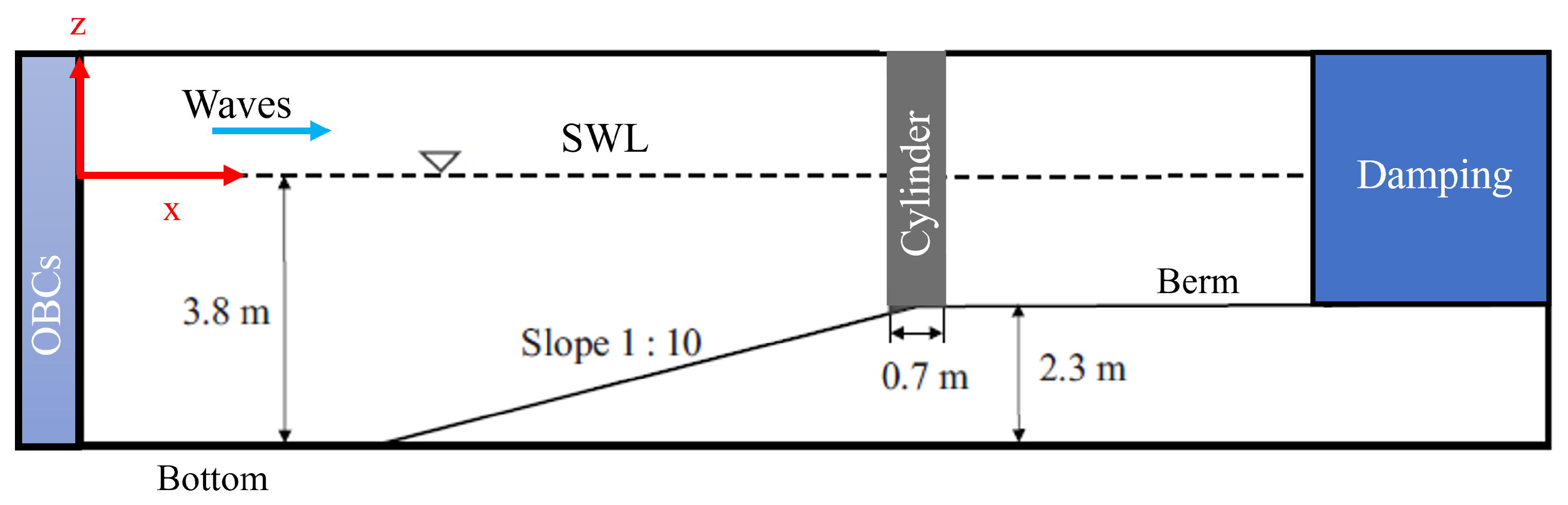
3.1. Experimental Setup and Wave Conditions

The experimental setup consisted of a slender cylindrical pile with a height of 5 m and a diameter of 0.7 m. The investigation also covered inclined positions of the cylinder at varying angles; however, these are not discussed here because they were not utilized for the validation of the numerical model. In addition, a sloping seabed with a gradient of 1:10 was constructed in the wave flume to induce depth-limited wave breaking, with the cylinder placed immediately behind this slope on a berm.

Regular waves were generated with wave periods varying from 3.0 to 10.0 s. The wave conditions for the specific case modeled here are intended to resemble those used in Li and Fuhrman [15]: wave period (T) equal to 4.0 s, incident wave height (H) of 1.3 m at wave generation, and water depth at generation equal to 3.8 m. The calculated surf similarity parameter (${\xi }_0$) is 0.42, which is indicative of an expected strong spilling, breaking scenario.

3.2. Numerical Setup

The numerical setup closely follows the experimental configuration outlined by [46] and is illustrated in Figure 1. The origin of the coordinate system is the numerical wave generation. The numerical wave flume has been shortened with respect to the experimental one to reduce the computational cost. However, the numerical setup and wave conditions employed in the SPH model resemble those used in the work presented by [15]. The x-axis indicates the propagation of waves, while the y-axis denotes the transverse direction. The pile is located midway between the two sides of the 5-meter-wide flume. The pile is located at $(x,y)=(27.0\mathrm{m},0.0\mathrm{m})$, while the numerical wave generation is located at $x=0.0$ m. Boundary conditions are enforced as follows: the generation of waves is facilitated by inlet/outlet conditions as in [56], and is achieved by using a stream function solution that draws from the contributions of Fenton’s research [60]. A wave-damping zone is applied on the right-hand side of the domain, at the outlet location, to reduce the wave reflection from the outlet buffer. We remark that the SPH formulation used in this investigation is single-phase, which implies that the air presence is not accounted for.

Three values of initial inter-particle distance have been investigated, namely, $\mathit{dp}=0.076\mathrm{m}$, $0.065\mathrm{m},\mathrm{and}0.05\mathrm{m}$, which lead to an initial particle count between 1.2 and 4.5 million. A value of 2.1 is predefined for the ratio h/dp. For all these resolutions, various dissipation schemes are applied, specifically the artificial viscosity, the laminar viscosity, and the laminar + SPS model. For the artificial viscosity model, a coefficient $\alpha =0.01$ is used following the recommendation in [52]. In DualSPHysics, the ViscoBoundFactor, or VBF, enables the multiplication of the viscosity between the fluid and boundary particles when the artificial viscosity model is applied with a value of VBF, which can range between 0 and 1 [61]. However, values in excess of 1 have also been used to enhance the numerical friction exerted by the boundary on the fluid particles [62,63]. In the present work, $VBF=0$, having verified that other values lead to a significant reduction in the exerted wave forces on the pile. The Fickian shifting algorithm developed by Lind et al. [64] is also used. Particles that discretize the base of the flume, the lateral walls, and the cylinder are mDBC particles [55]. A symplectic time-integration scheme is employed together with variable time stepping constrained by a Courant–Friedrich–Levy (CFL) condition with a coefficient 0.2 [65]. Version 5.4 of DualSPHysics is employed on an NVIDIA GeForce RTX 4090 GPU.

4. Model Validation Against Experimental Data

The present investigation focuses on the SPH framework, comparing three dissipation schemes: standard artificial viscosity, a laminar formulation without explicit turbulence modeling, and a laminar model supplemented with a sub-particle scale (SPS) turbulence approach. The ensuing results are presented in this section: wave breaking process, water surface elevation, and force history, alongside experimental data.

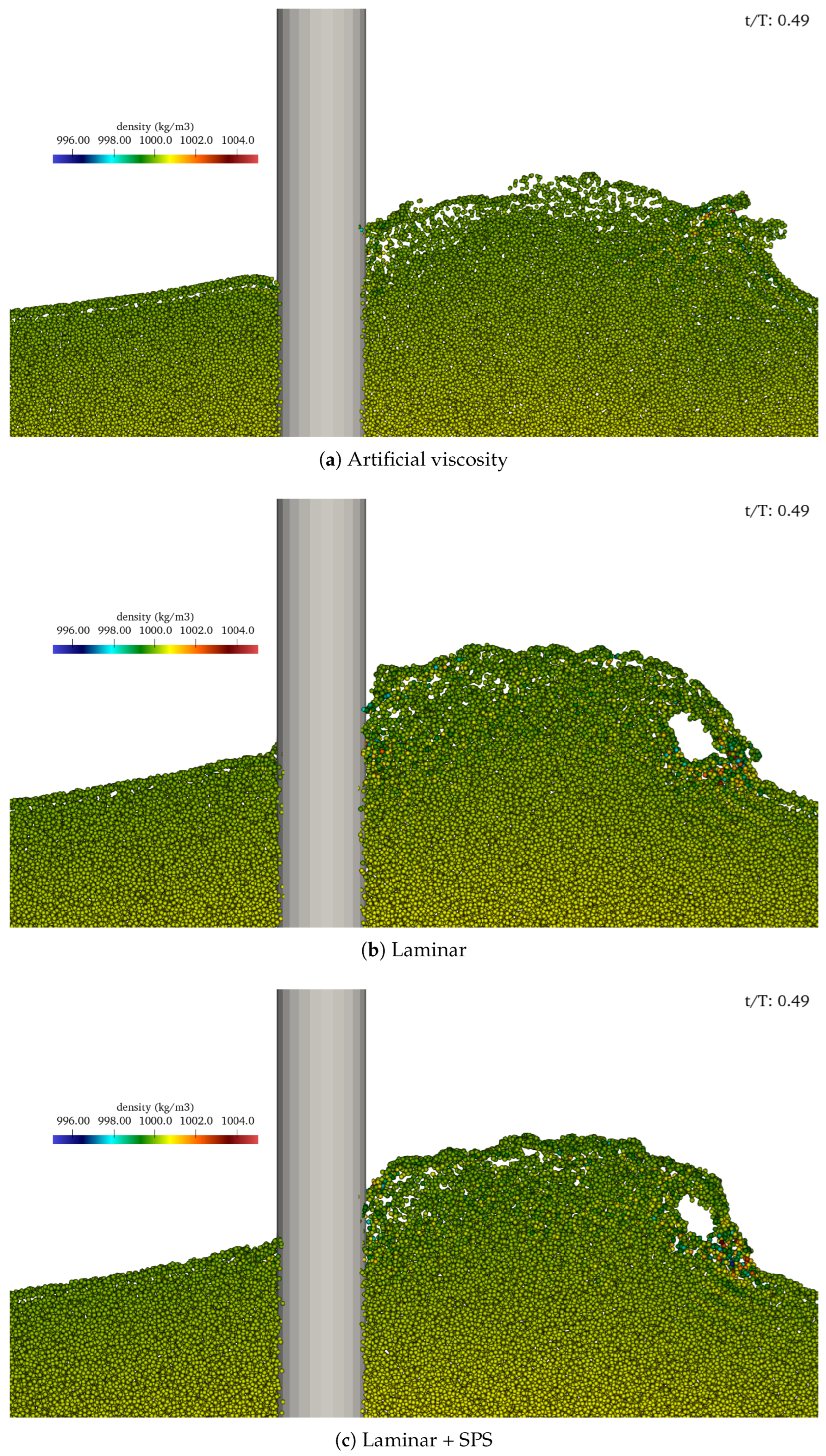
4.1. Evolution of Wave Breaking and Breaking Point

Figure 2 shows the horizontal velocity field at the free surface for the three dissipation schemes tested in the SPH framework. The left panels provide a top view of the velocity field, while the right panels show an isometric view that highlights the interaction between the breaking wave and the vertical cylinder. The snapshots correspond to the moment just before the breaking wave impact ($t/T\approx 0.28$, with $t/T=0$ defined at the seventh wave cycle, when the simulations reach a repeatable state), for the case with model resolution $\mathit{dp}=0.065\mathrm{m}$. The comparison illustrates the influence of the dissipative scheme on the velocity distribution and flow structure near the breaking point. In the AV simulation, the wave front appears significantly more diffused, with a smoother velocity gradient in the wave crest region. This is indicative of excessive numerical dissipation, which tends to dampen wave-breaking dynamics and reduce the flow intensity near the structure. The laminar model, in contrast, preserves sharper gradients in the velocity field, especially around the leading edge of the wave and pile impact zone, consistent with the finding in [15], which showed that a laminar model can be reasonably accurate at breaking onset. The laminar + SPS model maintains the sharpness of the wave front observed in the laminar case while also producing smoother, more physically consistent flow structures around the pile. The velocity field retains high intensity in the breaking region, but it limits the excessive damping seen with AV and the slight noise apparent in the purely laminar simulation. From the right panel of Figure 2, the free surface from the AV simulation appears flattened and lacks the three-dimensional flow structures associated with breaking waves. In contrast, the laminar and SPS-enhanced models reproduce more realistic breaking wave forms, with the SPS model showing well-structured crest overturning and more accurate representation of the impact zone on the pile. These results confirm that, while AV may be sufficient for general wave propagation, it seems to underestimate local flow dynamics during wave breaking and impact. The laminar + SPS model provides a more robust and physically consistent description of the near-surface horizontal velocity field, which is particularly important in applications involving wave–structure interactions. Notably, a slight shift in the timing of the wave impact on the pile is observed. In the AV simulation, the wave appears to impact the structure slightly earlier. This anticipated impact is caused by a numerical artifact introduced by artificial viscosity. Specifically, the dissipation smooths the wave crest and reduces its steepness, effectively altering the local wave nonlinearity and leading to a phase shift in the wave’s position relative to the experimental case. As a result, the crest reaches the structure prematurely in the simulation. This behavior is particularly evident in simulations with higher values of the artificial viscosity parameter, while the wave celerity apparently increases for lower values of $\alpha$, as illustrated in Appendix A and Figure A1. An additional comparison is made for the same case with $VBF=1$, where the excess of numerical dissipation between the fluid and bottom causes an important delay in the wave-breaking and impact process. This delay is consistent with the overall reduction in wave energy and speed due to numerical dissipation.

In Figure 3, the particle density distribution at $t/T=0.49$ is compared for the different dissipation schemes. Each subfigure uses a color scale from approximately 995 kg/m³ (blue) to 1005 kg/m³ (red), corresponding to a variation of about $\pm 0.4\%$ around the nominal 1000 kg/m³. Such density fluctuations are acceptable within the weakly compressible SPH framework, provided they remain spatially continuous and physically consistent with basic continuum-mechanics principles. In all three cases, the most pronounced density gradients occur near the impact zone at the free surface, where a plunging jet interacts vigorously with the fluid beneath, generating a strong local compression. Here, the density varies sharply within a very short spatial distance, reflecting numerical compressibility effects under high-acceleration conditions. Away from this impact region, the density has a more uniform distribution in the range of 999–1000 kg/m³, indicating no significant or spurious discontinuities in the calmer regions of the flow. Although these small deviations in neighboring particles can be less than fully representative of real-water incompressibility, they remain consistent with the transient nature of wave impacts and the weakly compressible methodology adopted. Overall, the observed density fields confirm that the numerical fluctuations, although present, are largely confined to regions of intense flow activity and do not degrade the physical plausibility of the global solution.

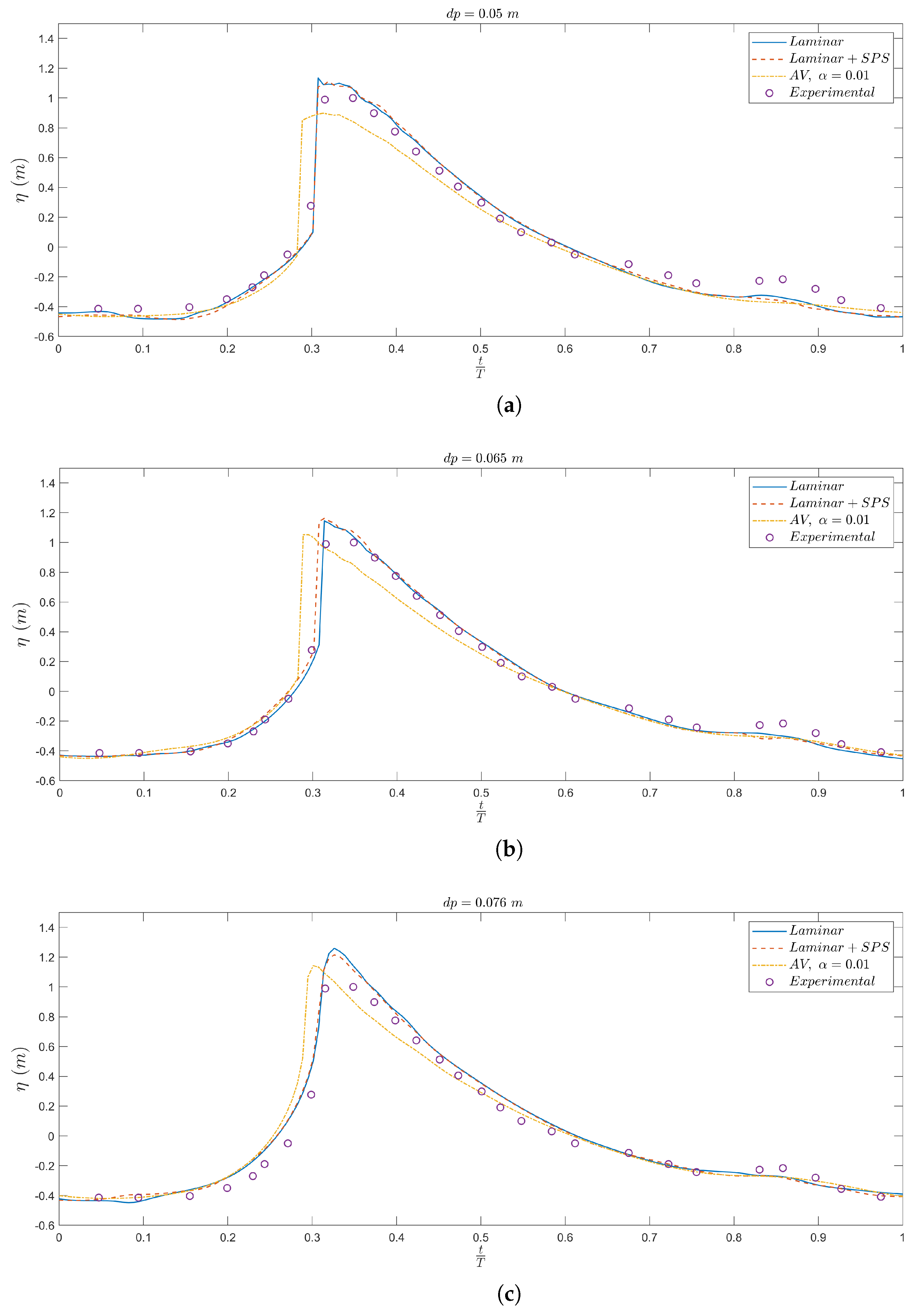
4.2. Free-Surface Elevation

The evolution of the water surface elevation is considered next and is investigated both from numerical and experimental results, using superimposed plots to elucidate any discrepancies and trends across different resolutions and modeling schemes.

Figure 4 presents the time series of free surface elevation, $\eta$, at the location $(x,y)=(27.0\mathrm{m},1.9\mathrm{m})$ for three different particle spacings: $\mathit{dp}=0.05\mathrm{m}$, $\mathit{dp}=0.065\mathrm{m}$, and $\mathit{dp}=0.076\mathrm{m}$. For each case, the numerical results obtained using the laminar model, the laminar + SPS model, and the artificial viscosity with $\alpha =0.01$ are compared with experimental measurements. Overall, both the laminar and laminar + SPS models reproduce the experimental wave profiles with high accuracy. The wave crest is captured sharply, and the arrival time of the wave front is consistent with the measurements. When SPS is used, a slightly smoother prediction is observed during the wave build-up and decay phases, particularly visible in the post-impact region. This is likely due to the additional sub-particle scale dissipation acting selectively in regions of high velocity gradients. In contrast, the finest resolution AV-based simulation underestimates the crest height and introduces an earlier but more gradual wavefront, resulting in a smoothed profile that deviates more significantly from the experimental data. The medium and lower resolution simulations still show a steep wavefront, while this time the results overpredict the experimental ones. This behavior reflects the artificial diffusion introduced by the AV model, which dissipates wave energy and reduces the steepness of the crest. The underestimation of the wave height is most evident for the highest resolution ($\mathit{dp}=0.05\mathrm{m}$), where the steepness of the wave front is greatest and the effect of AV-induced smoothing becomes more pronounced. Increasing the particle spacing from $\mathit{dp}=0.05\mathrm{m}$ to $\mathit{dp}=0.076\mathrm{m}$ leads to a minor loss in fidelity, particularly in the timing and sharpness of the crest. However, the general agreement with the experimental data remains acceptable across all resolutions for the laminar and laminar + SPS models, confirming the robustness of these formulations.

Figure 3. Particle density distribution at $t/T=0.49$. The color scale ranges from approximately 995 kg/m³ (blue) to 1005 kg/m³ (red), showing variations in fluid density around the cylinder.

Figure 3. Particle density distribution at $t/T=0.49$. The color scale ranges from approximately 995 kg/m³ (blue) to 1005 kg/m³ (red), showing variations in fluid density around the cylinder.

Figure 4. Time series of the free surface elevation $\eta$ at the location $(x,y)=(27.0\mathrm{m},1.9\mathrm{m})$ for three different particle spacings. Numerical results obtained using artificial viscosity (AV), laminar, and laminar + SPS models are compared against experimental data. Subfigures correspond to: (a) $\mathit{dp}=0.05$ m; (b) $\mathit{dp}=0.065$ m; (c) $\mathit{dp}=0.076$ m. The non-dimensional time $t/T=0$ is defined at the seventh wave cycle, when the simulation reaches a repeatable state.

Figure 4. Time series of the free surface elevation $\eta$ at the location $(x,y)=(27.0\mathrm{m},1.9\mathrm{m})$ for three different particle spacings. Numerical results obtained using artificial viscosity (AV), laminar, and laminar + SPS models are compared against experimental data. Subfigures correspond to: (a) $\mathit{dp}=0.05$ m; (b) $\mathit{dp}=0.065$ m; (c) $\mathit{dp}=0.076$ m. The non-dimensional time $t/T=0$ is defined at the seventh wave cycle, when the simulation reaches a repeatable state.

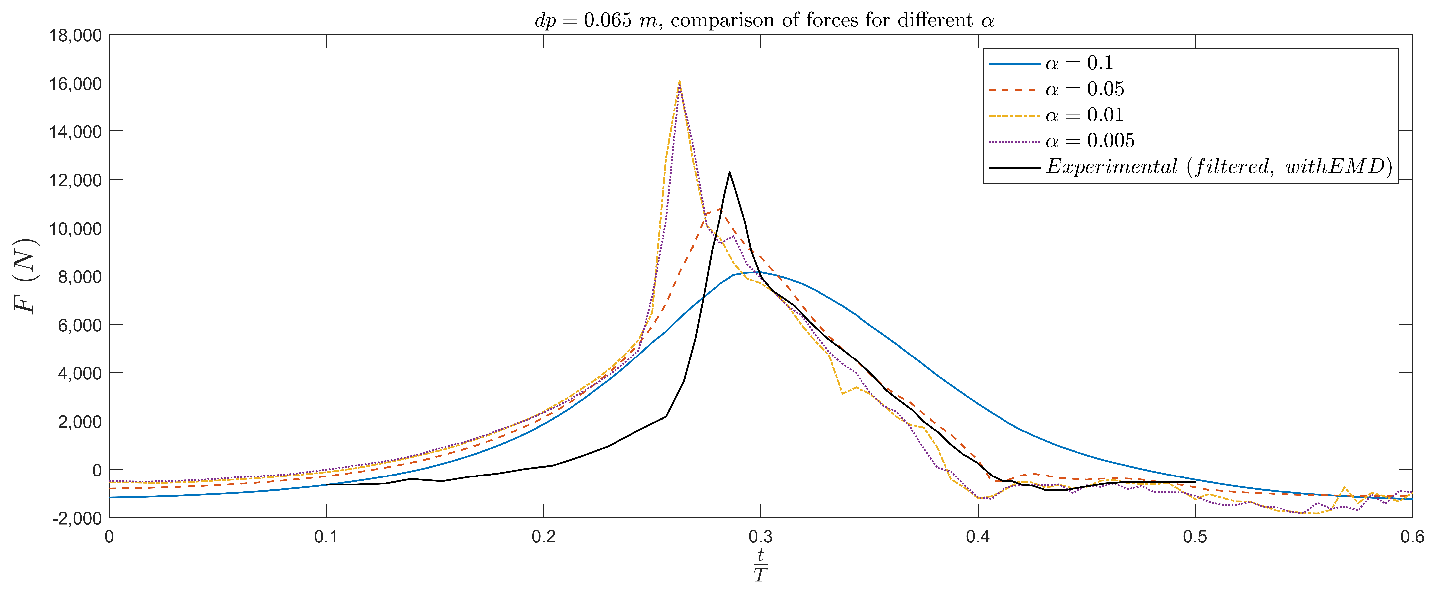
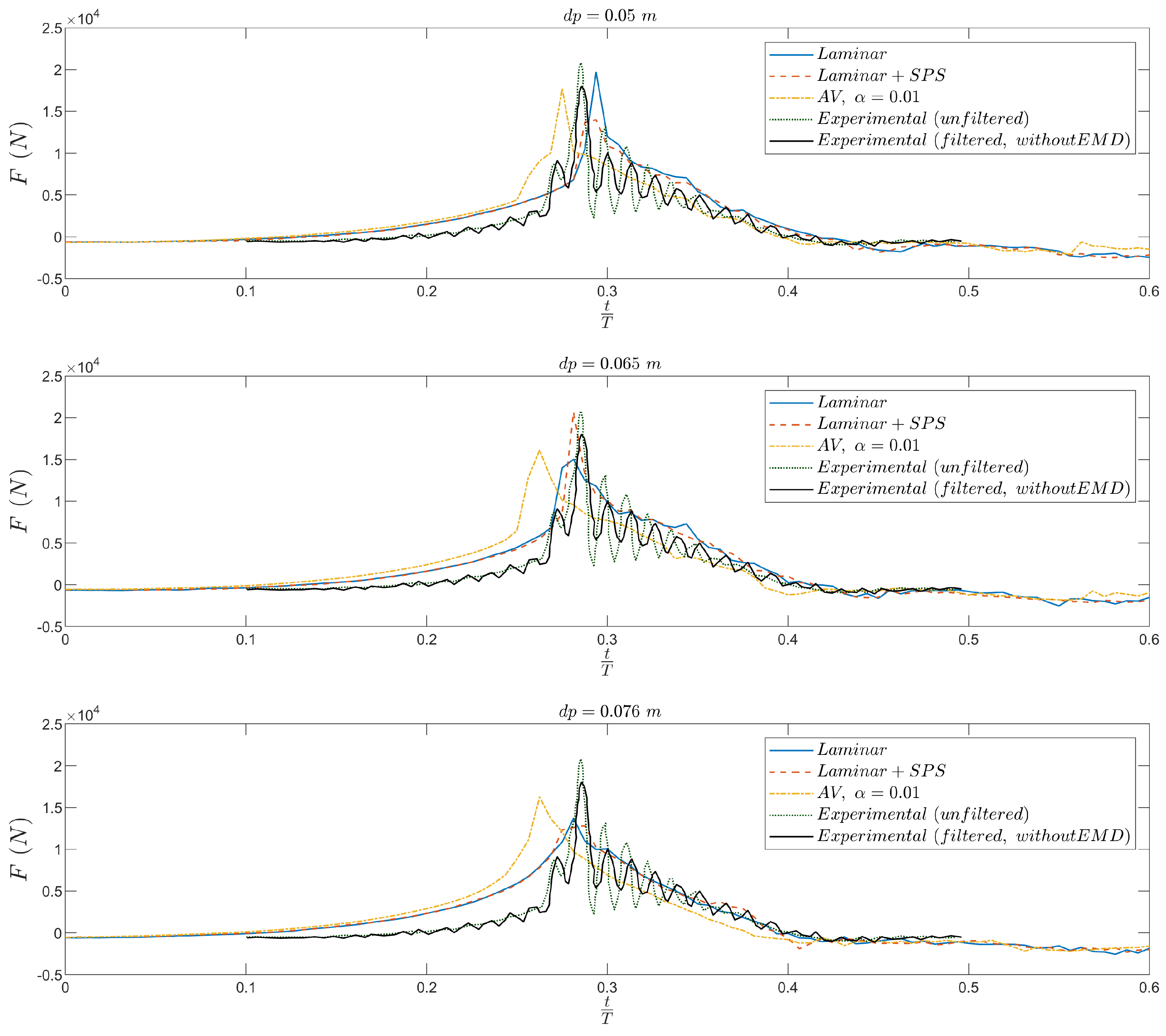
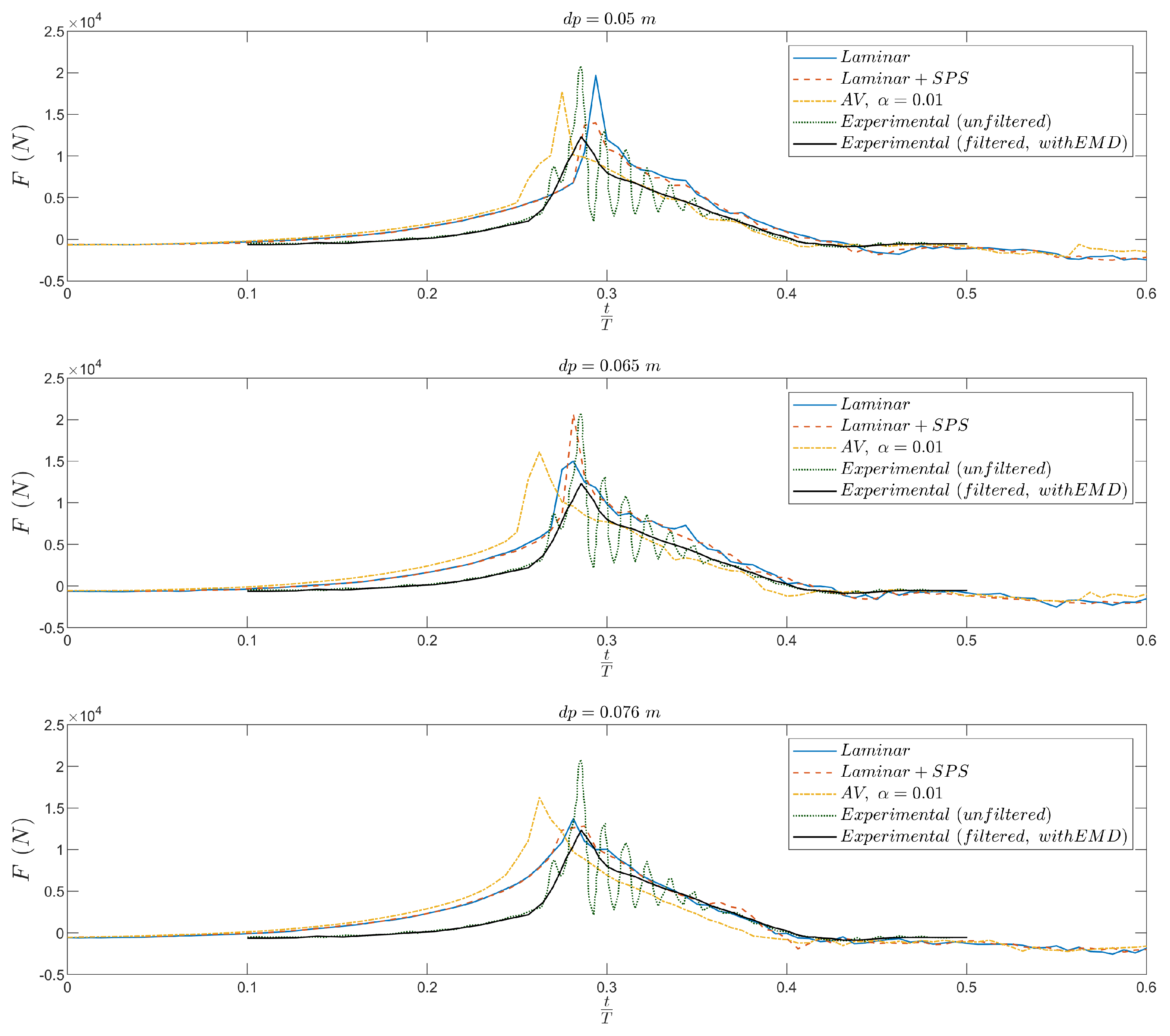
4.3. Slamming Force Prediction

Figure 5 and Figure 6 present the time evolution of the horizontal force, F, exerted by the breaking wave on the vertical pile for the same three dissipation schemes and spatial resolutions. The results are compared with the experimental data from [46], where force measurements were recorded using a sampling frequency of 200 Hz. To interpret the experimental signals, two levels of post-processing are considered, in agreement with the experimental analysis. In Figure 5, the raw experimental and low-pass filtered data (cut-off frequency of 20 Hz) are shown, the latter aiming to reduce the contribution of structural vibrations. In contrast, Figure 6 shows the same data with the additional application of empirical mode decomposition (EMD), where the envelope mean of the filtered signal is used to extract the net hydrodynamic force following the procedure in [66].

In both figures, the impact of the breaking wave appears clearly as a sharp peak around $t/T\approx 0.28$, where $t/T=0$ corresponds to the seventh wave cycle when the simulations reach a repeatable state. Across all resolutions, the laminar and laminar + SPS simulations reproduce the timing and amplitude of the impact force with a high degree of accuracy. The SPS model tends to slightly smooth the signal in the post-impact phase while maintaining accurate peak values, likely due to the additional sub-particle scale dissipation. The AV model, on the contrary, overpredicts the peak force compared to the experimental data with EMD, and exhibits a premature rise, especially at finer resolutions (e.g., $\mathit{dp}=0.05\mathrm{m}$), which can be attributed to the artificial dissipation affecting the wave dynamics and crest steepness: eventually the dissipation induced by the chosen value of the artificial viscosity coefficient is too little. Further considerations on the importance of $\alpha$ are reported in Appendix A.

When comparing Figure 5 and Figure 6, it is evident that the experimental signal processed with EMD (black solid line) provides a more stable and physically interpretable reference because it removes the residual, high-frequency oscillations observed in the raw and simply filtered signals. The EMD-processed curve reveals a well-defined and smooth impact peak that aligns closely with the laminar and SPS simulations, further supporting their accuracy.

A discrepancy in the rising time of the impact force is observed, where numerical simulations exhibit a more gradual force buildup compared to experimental measurements. This can be attributed to inherent features of the WCSPH method. In particular, the weakly compressible formulation employs an artificial speed of sound to approximate incompressibility, which introduces slight density and pressure diffusion. This may result in premature but less intense force development ahead of the slamming peak. Additionally, the SPH smoothing length h, which governs the spatial resolution of particle interactions, affects the sharpness of gradient capture. A larger $h/dp$ ratio, while beneficial for numerical stability, tends to smear steep fronts such as the approaching wave crest. These combined effects broaden the pressure field and elongate the force rise phase. Future work may investigate adaptive smoothing strategies or higher-order SPH formulations to reduce this pre-impact smoothing and better align with experimental dynamics.

Comparison of Slamming Forces with Li & Fuhrman [15]

Figure 6 highlights the ability of all numerical configurations to capture the impulsive nature of the slamming force associated with wave impact. The peak force duration, $t_D$, is approximately $0.02\mathrm{T}$, consistent with the experiments. In particular, the maximum force computed with the laminar + SPS model and $\mathit{dp}=0.05$ m reaches approximately $1.6\times {10}^4$ N, which is in excellent agreement with the peak value reported in [15], where a mesh-based approach was employed using the Reynolds stress–$\omega$ turbulence model. The effect of turbulence modeling on incipient wave breaking is made following findings in [15], which noted that when waves break incipiently on the leading face of a vertical cylinder, the predicted peak force remains essentially unchanged provided that the turbulence model is implemented in a stable and convergent manner. However, the present SPH simulations exhibit discernible differences in the predicted peak force and rising time, especially when the artificial viscosity model is used. Specifically, AV runs with $VBF=0$ and $\alpha =0.01$ overestimate the slamming magnitude and display early slamming, if compared to the laminar and laminar + SPS models, as well as the experimental measurements. When $VBF$ is set to 1, a substantially higher slamming force is obtained, accompanied by a considerable delay in the impact event (not presented here for the sake of brevity). These discrepancies suggest that, within the SPH framework, the artificial viscosity term necessitates precise, ad hoc calibration to enhance the accuracy of the SPH simulations in scenarios involving wave breaking.

We emphasize that [15] focused on mesh-based RANS simulations employing stable turbulence closures, such as the stabilized k–$\omega$ and stress–$\omega$ models, explicitly designed to avoid over-production of turbulence prior to incipient breaking. In these formulations, the crest flow remains predominantly laminar until it overturns, and the onset of breaking is not significantly altered by the choice of model. In contrast, the standard artificial viscosity approach in SPH produces numerical dissipation throughout the domain while serving to stabilize the particle motion. This results in a reduction of the wave crest steepness, even before overturning, and consequently a weaker or delayed slamming impact on the structure. The need for more advanced sub-particle scale turbulence models is thus important to avoid cumbersome AV fine-tuning [53,67], ensuring that rapid free-surface motion and crest overturning are captured in line with the local flow physics of wave breaking events.

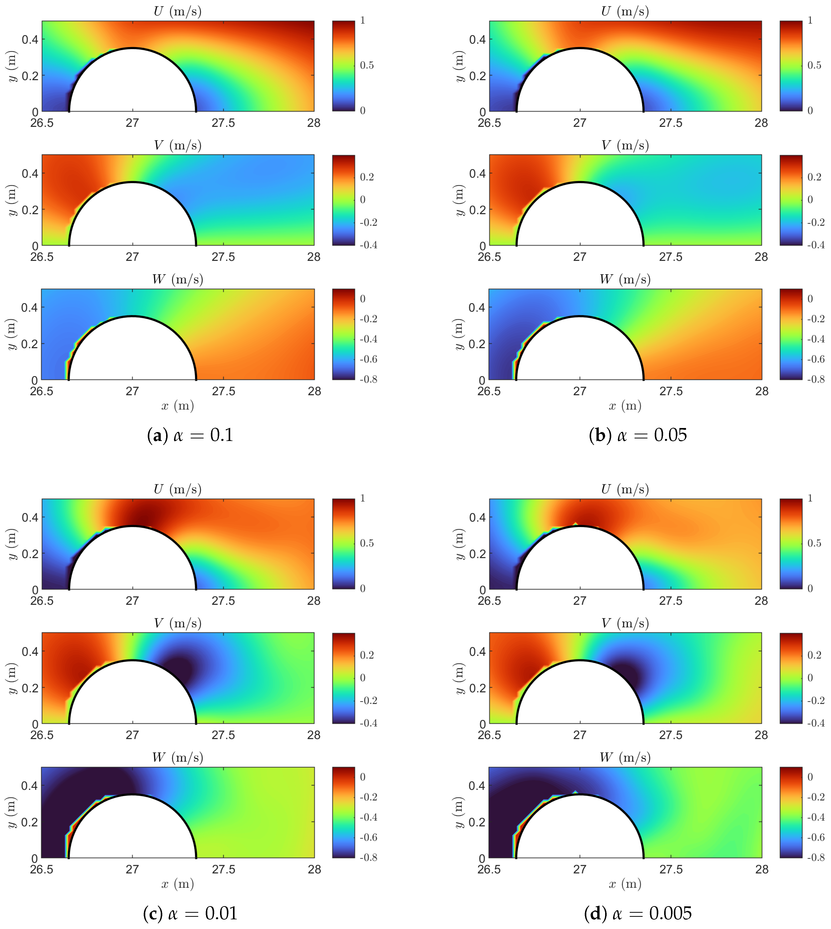
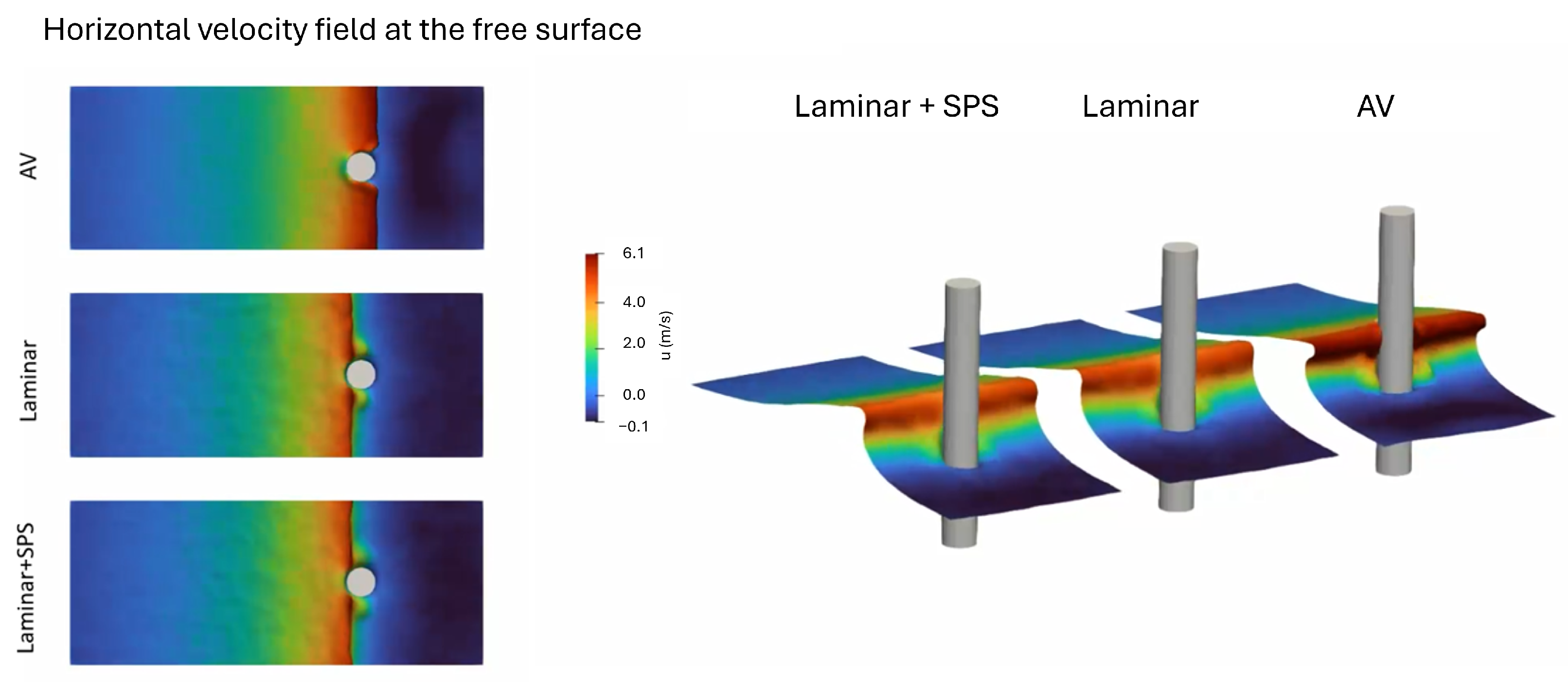
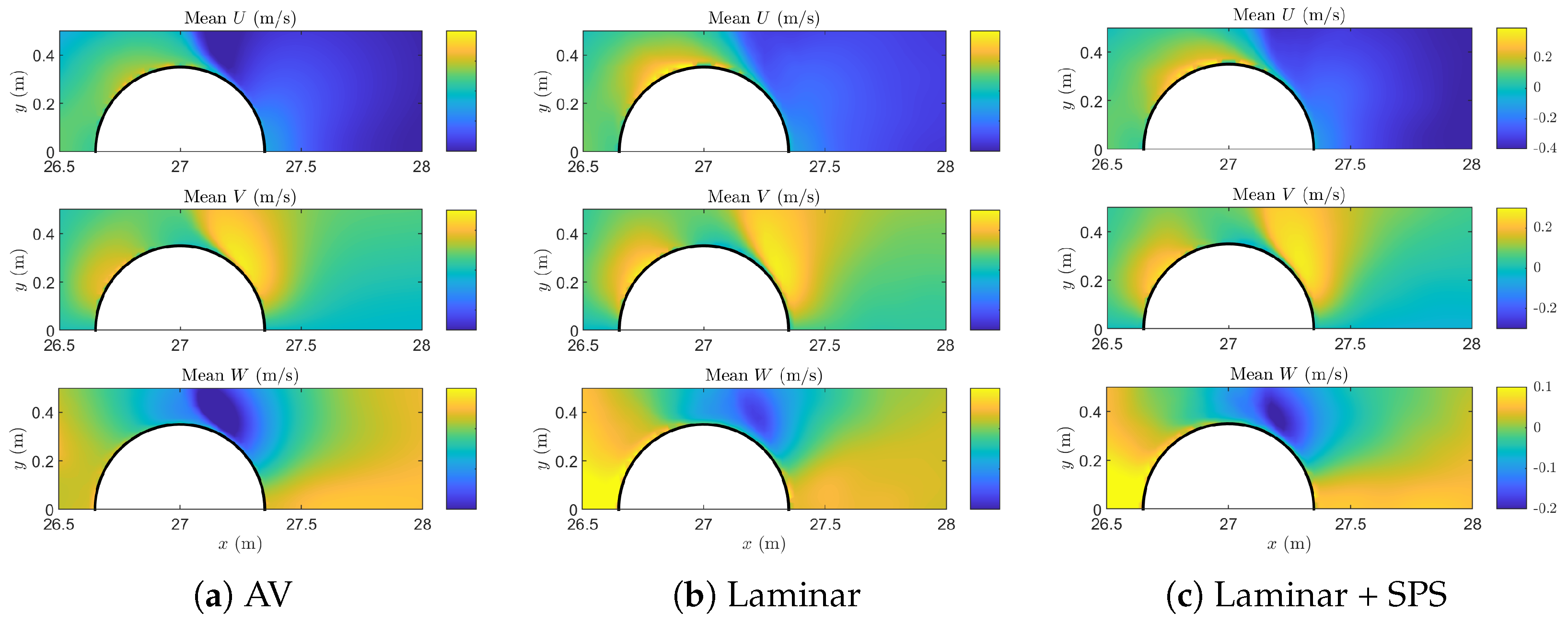
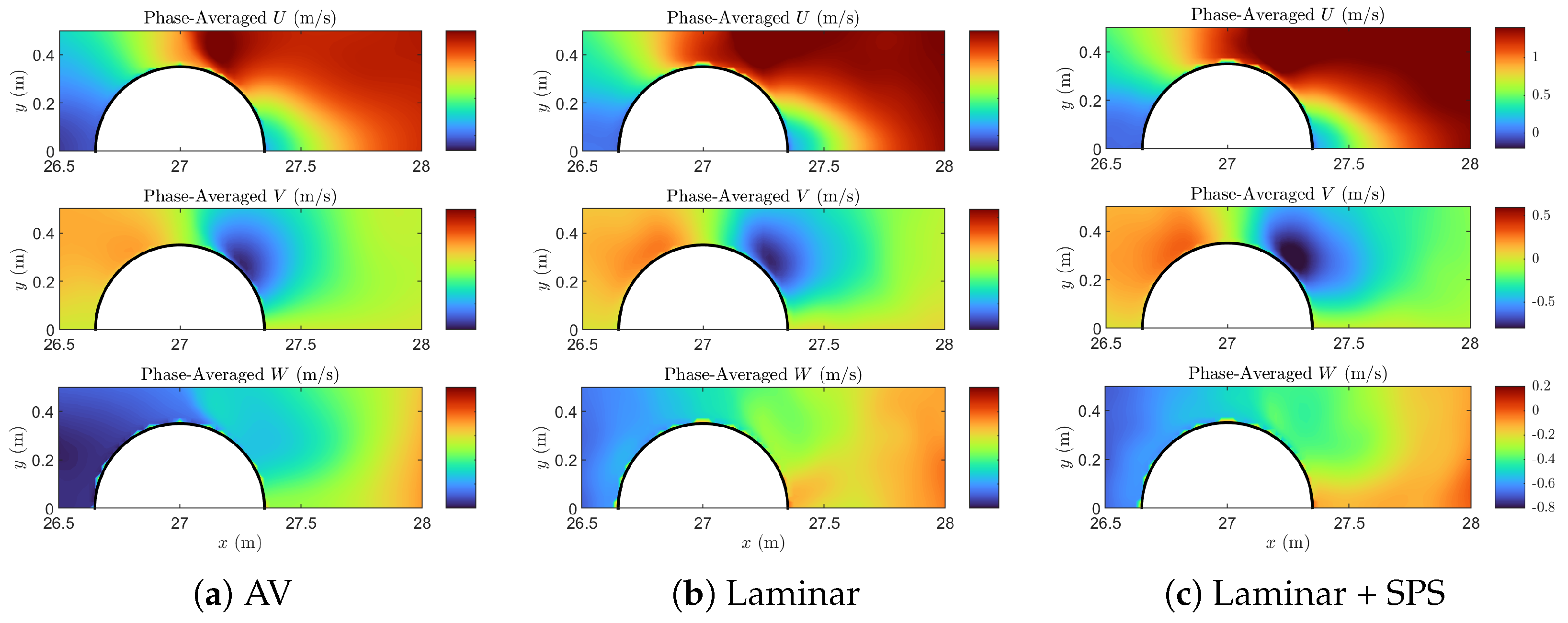
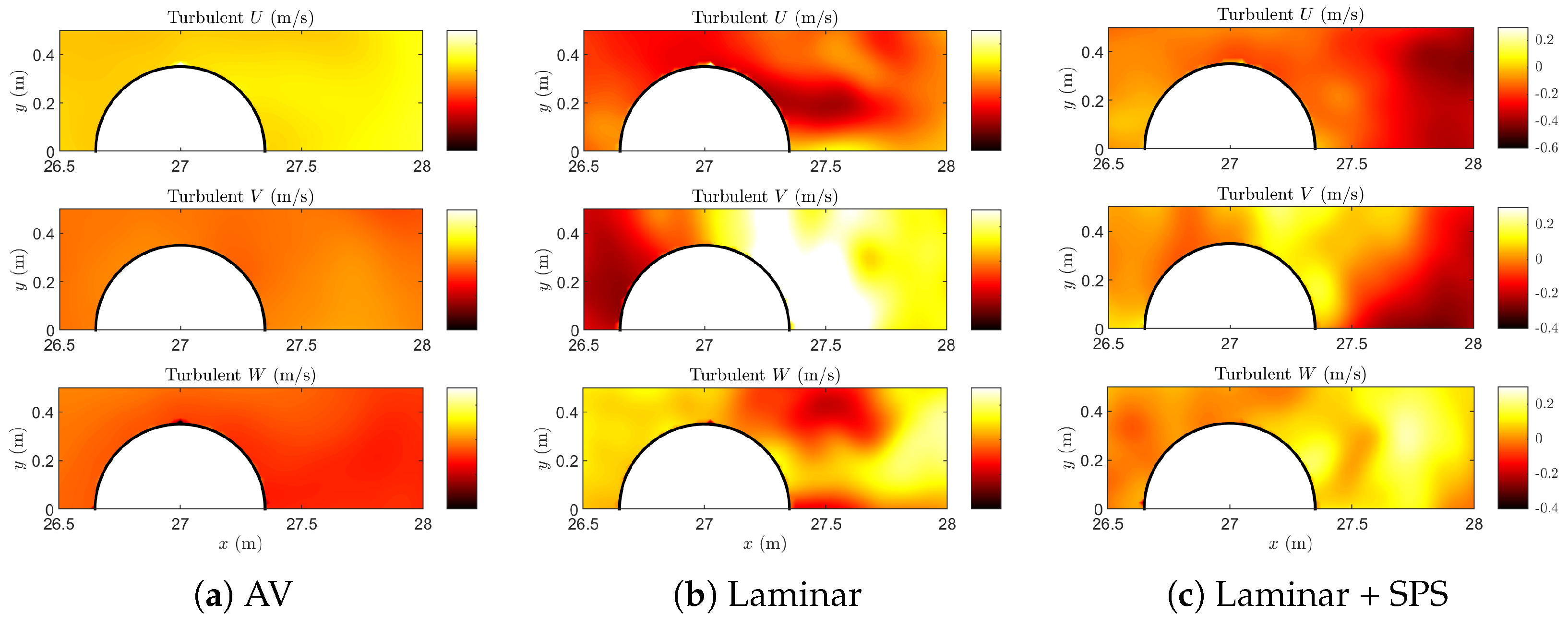
5. Velocity Field and Turbulence Characteristics

Herein, a detailed examination of the flow field is carried out, focusing on the mean and phase-averaged velocity and the turbulent velocity component. This is followed by a discussion of the distribution of turbulent kinetic energy (TKE) and coherent turbulent structures around the vertical pile.

5.1. Velocity Field Decomposition

To analyze the flow dynamics around the cylinder, we extract the mean velocity distributions, phase-averaged velocity profiles, and turbulent velocity fluctuations from the velocity field. The instantaneous velocity field $\mathbf{v}(\mathbf{x},t)$ obtained from the SPH simulations is decomposed into three components: the time-averaged (mean) field, the phase-averaged (coherent) field, and the residual (turbulent) fluctuations. The decomposition is expressed as follows:

$$\mathbf{v}(\mathbf{x},t)=\langle \mathbf{v}\rangle \left(\mathbf{x}\right)+\tilde{\mathbf{v}}(\mathbf{x},t)+{\mathbf{v}}^{″}(\mathbf{x},t),$$

(12)

where

• $\langle \mathbf{v}\rangle \left(\mathbf{x}\right)$ is the time-averaged velocity over several wave periods;
• $\tilde{\mathbf{v}}(\mathbf{x},t)$ is the phase-averaged velocity, representing the coherent, repeatable component associated with the wave motion;
• ${\mathbf{v}}^{″}(\mathbf{x},t)$ is the turbulent (incoherent) fluctuation, defined as the deviation from the phase-averaged field.

The variable $\tilde{\mathbf{v}}(x,t)$ can be expressed as follows:

$$\tilde{\mathbf{v}}(\mathbf{x},t)={\displaystyle \frac{1}{N}}\sum _{n=1}^N\mathbf{v}\left[t+(n-1)T\right]-\langle \mathbf{v}\rangle \left(\mathbf{x}\right),$$

(13)

where T is the wave period and N is the number of wave cycles. The summation averages the instantaneous velocity at the same phase t within each of the N wave periods. The averaging procedure was performed over seven full-wave cycles after the system reached a statistically repeatable state. The mean and phase-averaged fields were computed at corresponding phase instants in each cycle using the wave period T, while the turbulent velocity field was obtained as follows:

$${\mathbf{v}}^{″}(\mathbf{x},t)=\mathbf{v}(\mathbf{x},t)-\tilde{\mathbf{v}}(\mathbf{x},t)-\langle \mathbf{v}\rangle \left(\mathbf{x}\right).$$

(14)

The results shown hereafter refer to the highest model resolution, namely, $\mathit{dp}=0.05\mathrm{m}$. The time $t/T=0.49$ is chosen to favor an easier comparison with results in [15]. Figure 7 presents the instantaneous velocity fields for the three velocity components, U, V, and W, extracted at mid-depth ($z=-D/2$), comparing the three dissipation schemes. The results of the AV model in Figure 7a show a relatively smooth and diffused flow pattern, especially for V and W. The horizontal velocity, U, exhibits a gentle transition around the cylinder, with a low gradient and relatively uniform distribution in the downstream region. The smoothing introduced by the AV model is expected to suppress the formation of coherent vortical structures. The laminar model in Figure 7b depicts more variation in the velocity field, with larger velocity gradients behind the cylinder, although the updated V field appears smoother than previously described, with milder cross-stream velocity variations and limited structure. In general, the flow pattern indicates the presence of more defined wake dynamics and cross-stream motion compared to AV. Nevertheless, it is hypothesised that this result is underpredicted (compared to that in Figure 7c), as resolving the turbulence with a laminar model would require refining the computational mesh and time step to the level of a direct numerical simulation (DNS). This, however, is not a viable option for the present 3D wave–structure interaction case. Looking at the laminar flow with the addition of the SPS model in Figure 7c, all three components show more spatial variability, with clear indications of energetic flow features around and behind the cylinder. The V and W distributions reveal intense cross-flow and vertical motion, respectively, suggesting stronger vortical activity and more energetic wake dynamics. The U field presents sharper gradients across the wake, indicative of enhanced turbulence mixing. The coherent structures are more in line with the physical expectations of the wave–structure interaction under a breaking wave impact. In general, these results highlight how the turbulence treatment affects the instantaneous velocity distribution. While the AV model leads to excessive smoothing, the laminar and especially the laminar + SPS models preserve sharper flow features and more physically representative dynamics. This supports the need for accurate turbulence models in SPH to capture the complex and transient nature of wave–structure interactions.

Figure 8 shows the mean velocity fields for the three velocity components $\langle \mathbf{U}\rangle$, $\langle \mathbf{V}\rangle$, and $\langle \mathbf{W}\rangle$ at mid-depth ($z=-D/2$). In this complex 3D scenario, the steady-state mean velocity contours reflect time-averaged flow characteristics resulting from repeated wave-induced impacts and subsequent flow separation around the pile. All three dissipation schemes clearly capture the upstream deceleration of fluid induced by the presence of the pile, followed by the formation of a wake region downstream. Specifically, the artificial viscosity (AV) scheme shows a slightly earlier and smoother flow separation around the lateral edges of the pile, indicated by relatively gradual gradients in the streamwise velocity. This leads to a more diffused and less clearly defined wake downstream, suggesting that wave-induced flow structures are somewhat excessively smoothed. In contrast, the laminar and, particularly, the laminar + SPS schemes predict a later and more localized separation region around the pile circumference. This delayed separation is reflected by sharper velocity gradients immediately behind the pile, indicating better preservation of coherent shear layers and, consequently, a narrower and more structured wake region. This refined prediction of flow separation is essential to capture realistic wave-induced forces, vortex shedding dynamics, and associated structural responses.

Figure 9 shows the phase-averaged velocity components at $t/T=0.49$ and mid-depth ($z=-D/2$). The phase-averaged fields represent the repeatable, wave-coherent motion of the fluid, filtered from turbulent fluctuations and numerical noise by averaging over seven wave cycles. The streamwise component $\tilde{U}$ displays the expected acceleration toward the pile and the deceleration in the wake region. All three models show a strong velocity gradient near the cylinder front, but the laminar and laminar + SPS models exhibit a slightly sharper transition, particularly close to the cylinder edge. The vertical component $\tilde{W}$ reveals a downward jet behind the cylinder, indicative of plunging wave behavior at this instant. The AV model again shows a milder pattern with lower peak magnitudes. The cross-stream component V also highlights significant differences. In both the laminar and laminar + SPS models, the component $\tilde{V}$ shows a strong lateral divergence around the pile, with a pronounced negative region downstream. This is associated with the side ejection of fluid induced by flow separation. The AV model captures the general trend but with attenuated magnitude and more diffused contours.

Figure 10 shows the turbulent velocity components $u^{″}$, $v^{″}$, and $w^{″}$. These fields represent the incoherent, high-frequency motion associated with turbulence and numerical fluctuations. The AV model shown in the left column of Figure 10 highlights how turbulence is highly suppressed, with little spatial velocity fluctuations, due to the inherent artificial damping. Specifically, the component $u^{″}$ only shows small patches of activity close to the wave impact zone on the pile crest. Moreover, the components $v^{″}$ and $w^{″}$ remain weak and spatially limited, with little structure, reflecting the over-diffusive nature of the artificial viscosity model. The laminar model in the center column of Figure 10 reveals moderately higher turbulent fluctuations than AV, particularly in $u^{″}$ and $w^{″}$ near the downstream side of the cylinder. The $v^{″}$ component, however, appears significantly weak, with minimal lateral fluctuation bands and only faint turbulence signatures in the wake. The $w^{″}$ field shows some vertical motion behind the cylinder, although it still lacks coherent patterns. These features appear somewhat irregular and unstructured, as expected from the absence of a dedicated turbulence model. The laminar + SPS model in the right column of Figure 10 displays the highest levels of turbulent kinetic energy (see also Figure 11), with better-organized structures. The components $u^{″}$ and $v^{″}$ exhibit clear fluctuations on both sides of the pile, indicating cross-flow instability and wake unsteadiness. The $u^{″}$ distribution is particularly intense in the wake, while $v^{″}$ reveals alternating bands of fluctuation indicative of lateral shear. The component $w^{″}$ presents stronger vertical motions, particularly above the cylinder, where plunging-induced vortices form. Compared to the other models, the SPS-enhanced simulation yields improved spatial coherence and magnitude in all components, capturing more realistic turbulence generation and transport. The spatial coherence of the turbulent structures is improved compared to the laminar case, suggesting that the SPS model improves the resolution of shear-driven instabilities.

The turbulent velocity fluctuations computed from Equation (14) do not correspond to turbulence as resolved in direct numerical simulation (DNS), because the particle spacing and time step in the present SPH simulations are significantly larger than the Kolmogorov scales. Nonetheless, recent studies have shown that SPH can capture meaningful turbulent flow features, such as coherent structures and bulk velocity statistics, even at coarse resolution, provided the interpretation is consistent with filtered or ensemble-averaged turbulence representations [68,69]. In this study, the observed velocity fluctuations reflect sub-resolved flow dynamics and serve as indicators of energetic regions such as wake separation, wave impact zones, and vortex shedding. Similarly, while the SPS model used here (Equation (10)) formally resembles the Smagorinsky sub-grid model from LES, the relatively coarse particle resolution limits its ability to model turbulence in a rigorous LES sense. Although not resolving sub-particle turbulence explicitly, the SPS model enhances physical realism compared to artificial viscosity and laminar-only formulations. Future work may explore adaptive resolution [70] to improve turbulence modelling fidelity.

The comparison of velocity fields across the three dissipative schemes highlights substantial differences in the ability of each model to represent the flow dynamics around the vertical cylinder. AV systematically smooths out flow structures, leading to overly diffused mean and phase-averaged velocity fields and underprediction of turbulent fluctuations. Although it provides numerical stability, this approach suppresses important flow features such as separation zones, vertical jets, and lateral eddies. The laminar model captures realistic wave-induced motion, as evidenced by sharper gradients in the phase-averaged fields and stronger recirculation in the mean flow. It also allows for the emergence of turbulence through natural shear instabilities, though the resulting turbulent fields tend to be irregular and lack structure, although the results predicted with a laminar viscosity model (without turbulence modelling) may not be accurate post-wave breaking. In contrast, the laminar + SPS model improves both the organization and intensity of turbulent and coherent components, producing clearer flow separation, stronger wake dynamics, and more coherent vertical and lateral structures. The mean, phase-averaged, and turbulent velocity fields computed with this latter model are more consistent with physical observations of breaking wave impacts on vertical structures, supporting its suitability for accurate SPH simulations of wave-–structure interaction phenomena.

A notable aspect of the artificial viscosity model is its two-fold influence on the flow and resulting impact forces. High values of the coefficient ($\alpha$) generally induce substantial numerical diffusion, causing a smoother and more dissipative flow field. This diffusion leads to a reduced steepness of the wave crest and can delay or weaken the overall breaker impact. The ViscoBoundaryFactor (VBF) also plays an important role in modulating the viscous interaction between the fluid and the boundaries, e.g., seabed or pile. When $VBF$ is set to higher values, increased friction near the boundary can slow the fluid in the vicinity of the cylinder, potentially altering the impact force. In contrast, low $VBF$ values reduce boundary layer dissipation, allowing the fluid to retain higher velocities upon reaching the structure, sometimes resulting in larger impact loads. In practice, this balance between the artificial viscosity $\alpha$ in the bulk flow and the $VBF$ near the boundaries can yield contrasting scenarios. Even if the fluid is globally diffusive and smoothed by AV, a sufficiently low $VBF$ can preserve stronger wave speeds and produce a more energetic impact, while a large $VBF$ can introduce increased near-wall friction that damps the flow prior to collision. Therefore, careful calibration of $\alpha$ and $VBF$ is necessary to ensure realistic wave propagation, crest behavior, and structural forces under strong wave-breaking conditions.

5.2. Turbulent Kinetic Energy Distribution

The development of turbulence during the wave–structure interaction is further assessed by analyzing the turbulent kinetic energy (TKE) field at a horizontal plane located at $z=-D/2$. Figure 11 shows a comparison between the laminar and laminar + SPS simulations of a wave propagating to the right at two key instants: $t/T=0.34$, corresponding to the onset of the slamming phase, and $t/T=0.49$, marking the end of the impact.

At $t/T=0.34$, shortly after the wave front impacts the front face of the cylinder, both cases exhibit elevated TKE values near the upper part of the structure. The laminar case in Figure 11a shows that the TKE field remains highly localized, with a distinct peak on the rear side of the cylinder and a rapid decay away from the structure. In contrast, the laminar + SPS case in Figure 11b shows a more widespread and diffuse distribution of TKE, which extends downstream of the cylinder and reveals the formation of turbulent structures and enhanced mixing. This indicates that the SPS model works well with strong velocity gradients and captures additional energy from the unresolved scales, which is consistent with the expected behavior of subgrid turbulence during slamming. Furthermore, in the laminar simulation, the observed flow inversion likely arises from a strong local recirculation developing around the cylinder in the absence of significant turbulence. In other words, although the wave itself propagates from left to right, the relatively low effective viscosity in a purely laminar model can favor the early formation of a coherent recirculation bubble on the cylinder’s lee side, ultimately leading to velocity vectors oriented opposite to the main wave direction. By contrast, when the sub-particle scale (SPS) turbulence model is included, enhanced mixing and additional momentum exchange act to dampen or delay this flow reversal, keeping the velocity field more closely aligned with the incoming wave.

At $t/T=0.49$, when the impact has occurred, a more unexpected behavior is observed. The laminar simulation in Figure 11c shows significantly higher TKE values than the laminar + SPS case, with peaks in the upper-right region downstream of the cylinder. The TKE distribution is broader, and the velocity field shows signs of swirling motion and wake development. This suggests that, even without a turbulence model, strong unsteadiness and velocity gradients in the post-impact flow are sufficient to generate resolved-scale turbulence. In contrast, the laminar + SPS simulation (Figure 11d) exhibits a smoother flow field and noticeably lower TKE values. The energy remains confined near the cylinder’s surface with little evidence of developed wake turbulence at this instant. This discrepancy may be explained by a slight time shift between the two simulations: in highly impulsive flows, such as slamming, small phase mismatches can significantly alter the apparent turbulence intensity at a given nominal time. Alternatively, the SPS model may dampen or redistribute early turbulence more gradually, delaying the formation of sharp peaks in TKE.

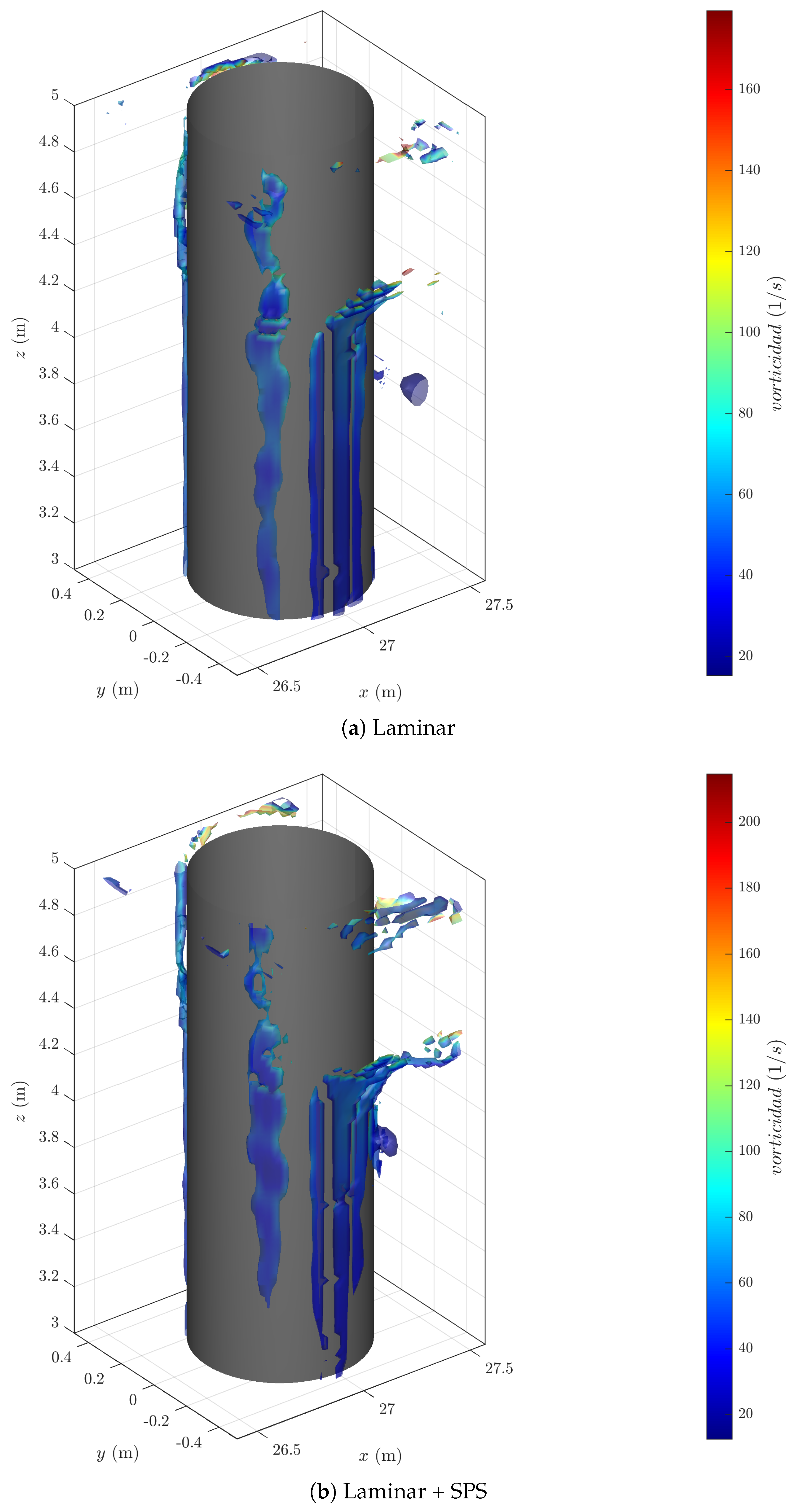
5.3. Coherent Structures

Identification of coherent turbulent structures in the flow field is carried out using the Q-criterion, which highlights regions where the rotation rate dominates over the strain rate. Mathematically, Q is defined as follows:

$$Q={\displaystyle \frac{1}{2}}\left({\parallel \mathbf{\Omega }\parallel }^2-{\parallel \mathbf{S}\parallel }^2\right),$$

(15)

where $\mathbf{\Omega }$ is the antisymmetric part (vorticity tensor) and $\mathbf{S}$ is the symmetric part (strain rate tensor) of the velocity gradient tensor. Regions with positive Q values represent vortical structures, making this criterion especially suitable for detecting flow instabilities and vortex shedding. In this study, the isosurfaces of $Q=50{\mathrm{s}}^{-2}$ are chosen to track the development and evolution of coherent structures induced by wave breaking and the wave–structure interaction.

Figure 12 shows the isosurfaces of the Q-criterion at time $t/T=0.34$, highlighting coherent vortical regions around the cylinder as the wave propagates from left to right. Figure 12a corresponds to the laminar simulation, while Figure 12b shows the laminar + SPS case. Even at this early stage of flow separation, significant differences arise in both the shape and concentration of coherent structures. The laminar scheme yields tall, columnar vortical filaments that extend vertically along the cylinder. These streak-like formations indicate strong flow detachment following the initial impact. Despite the absence of a turbulence model, the impulsive nature of wave loading generates velocity gradients large enough to produce resolvable vortical structures. In the laminar + SPS simulation, the vortex tubes are more fragmented and distributed around the mid-section of the cylinder, suggesting that the sub-particle scale (SPS) model is more effective in diffusing or breaking up large filaments. The flow exhibits broader, more dispersed patches of swirling motion, consistent with enhanced small-scale turbulence. Overall, the laminar simulation retains elongated vortex sheets, while the laminar + SPS simulation breaks them into smaller-scale eddies, underscoring how sub-grid modeling can influence the shape and distribution of coherent vortices in impulsive wave–structure interactions. While these turbulent coherent structures are not exact, they are included to provide additional context and transparency in relation to our results.

6. Discussion of Model Performance and Limitations

A comparative analysis is performed to discuss the performance of different diffusive schemes and resolutions in capturing key hydrodynamic features. The trade-offs between computational cost, numerical stability, and accuracy are evaluated. In particular, the laminar and laminar + SPS models demonstrate robust predictions of wave kinematics and breaking-induced forces, showcasing good convergence with experimental data over multiple spatial resolutions. In contrast, the artificial viscosity model exhibits excessive smoothing of velocity gradients, which results in lower wave crests for the finest model resolution, and a force impact that is not necessarily dampened, but rather shifted in phase, appearing earlier or more gradual compared to experimental observations.

Decomposing the instantaneous velocity field into mean, phase-averaged, and turbulent components highlights that AV overly diffuses both coherent wave structures and turbulence generation. Meanwhile, the laminar + SPS solution captures strong velocity gradients around the pile and more realistic turbulent fluctuations, yielding improved wake dynamics and flow separation patterns. The isosurfaces of the Q-criterion corroborate this result, showing more pronounced coherent structures in the laminar + SPS case, while AV simulations severely underestimate vortex formation.

Limitations remain with the current SPH implementation. Numerical diffusion is observed even when using the laminar and laminar + SPS models. Boundary treatment near the structure is also seen to introduce inaccuracies in shear layers and near-wall velocities.

7. Conclusions

Accurate simulation of fluid flow around vertical cylinders is essential for the design and assessment of offshore structures, bridge piers, and coastal defenses. Vertical piles are fundamental structural elements in marine environments, and understanding how they interact with waves is necessary to ensure their stability and longevity. The dynamics of breaking waves are complex and remain an active area of research, while the increasing occurrence of extreme weather events highlights the need for reliable simulations of severe hydrodynamic conditions, especially those involving breaking waves.

This study investigates the impact of wave breaking on a vertical pile using the SPH-based DualSPHysics model. The research specifically focuses on evaluating the performance of different dissipation schemes within the SPH framework, namely the artificial viscosity, the laminar viscosity, and a laminar viscosity model enhanced with a sub-particle scale (SPS) turbulence model. To assess the effectiveness and accuracy of these schemes, the numerical results are compared with large-scale experimental data in [46]. The study also examines how these different dissipation approaches affect the hydrodynamic forces acting on the pile, energy dissipation within the fluid, and the representation of flow characteristics such as wake structures, velocity fields, and turbulence. In addition, the influence of numerical resolution on the simulation results is considered. The ultimate goal is to contribute to the broader application of SPH in engineering design and hazard assessment related to coastal and offshore structures. This investigation builds on previous computational fluid dynamics studies that have emphasized the importance of turbulence modeling in predicting wave-induced forces on vertical piles.

Artificial viscosity (AV), while effective in stabilizing the simulations, introduced excessive numerical dissipation, leading to an overly diffused wave front and overpredicted peak slamming forces. In contrast, the laminar viscosity model produced sharper velocity gradients and more distinct wake features, providing more accurate reproduction of the timing and amplitude of wave impact forces without a dedicated turbulence model. The laminar + SPS approach explicitly accounted for sub-particle scale turbulence, and it retained the sharpness of the wave front observed in the laminar simulations with higher turbulence levels, more coherent vortex structures, and improved agreement with mesh-based RANS results, particularly for slamming forces.

Unlike the artificial viscosity model, which requires case-specific calibration of the dissipation coefficient $\alpha$, the laminar + SPS approach achieves higher fidelity using physically defined parameters. The kinematic viscosity ${\nu }_0$ is based on the physical properties of water, while the filter width $\Delta$ is typically set equal to the initial distance between particles, as commonly adopted in SPH turbulence modeling. These parameters are not tuned to match experimental results, but rather chosen to maintain physical consistency and numerical robustness.

These findings underscore the critical role of incorporating appropriate dissipation mechanisms in SPH simulations of wave breaking on marine structures. Although AV can ensure numerical robustness, its over-dissipative nature may adversely affect predictions of flow features and impact forces. In contrast, the laminar + SPS model stands out as a more suitable option for accurately resolving complex energy-transfer processes and turbulence characteristics in breaking-wave interactions. Future work will focus on refining SPS formulations and boundary treatments to enhance near-wall flow predictions, thereby advancing the reliability and applicability of SPH in coastal and offshore engineering contexts.

References

1. Alsultani, R.; Karim, I.; Khassaf, S.; Al-Saadi, A.A. Dynamic Response Analysis of Coastal Bridge Members Exposed to Water Forces and Earthquakes. In Advances in Civil Engineering; Bahadori-Jahromi, A., Ed.; IntechOpen: Rijeka, Croatia, 2024; Chapter 3. [Google Scholar] [CrossRef]
2. Han, W.; Zhou, K.; Wang, J.; Xiao, L.; Xu, X.; Xiang, Y.; Yu, X. Experimental Study of Wave Load Distributions on Pile Groups Affected by Cap Structures and Pile Spacings Under Varied Wave Conditions. J. Mar. Sci. Eng. 2024, 12, 2005. [Google Scholar] [CrossRef]
3. Hong, C.; Lyu, Z.; Wang, F.; Zhao, Z.; Wang, L. Wave-Current Loads on a Super-Large-Diameter Pile in Deep Water: An Experimental Study. Appl. Sci. 2023, 13, 8859. [Google Scholar] [CrossRef]
4. Li, M.; Leng, S.; Wang, Y.; Xue, S.; Wang, J.; Xu, G.; Mitoulis, S.A. Hydrodynamic analysis of bridge piers subjected to extreme waves. Proc. Inst. Civ. Eng. Bridge Eng. 2024. [Google Scholar] [CrossRef]
5. Chaplin, J.R.; Rainey, R.C.T.; Yemm, R.W. Ringing of a vertical cylinder in waves. J. Fluid Mech. 1997, 350, 119–147. [Google Scholar] [CrossRef]
6. Wienke, J.; Oumeraci, H. Breaking wave impact force on a vertical and inclined slender pile—theoretical and large-scale model investigations. Coast. Eng. 2005, 52, 435–462. [Google Scholar] [CrossRef]
7. Jiang, X.; Yin, Z.; Wang, Y.; Zhang, R. Group interaction effect on breaking wave forces on a vertical pile: Experimental tests and predictive models. Coast. Eng. 2025, 195, 104651. [Google Scholar] [CrossRef]
8. Petrini, F.; Manenti, S.; Gkoumas, K.; Bontempi, F. Structural Design and Analysis of Offshore Wind Turbines from a System Point of View. Wind Eng. 2010, 34, 85–107. [Google Scholar] [CrossRef]
9. World Meteorological Organization. Extreme weather and climate events. In State of the Global Climate 2023; United Nations: New York, NY, USA, 2024; pp. 23–25. [Google Scholar]
10. Altomare, C.; Gironella, X.; Marzeddu, A.; Viñes Recasens, M.; Mösso, C.; Sospedra, J. Impact of focused wave groups on pier structures: A case study of severe breaking waves at Pont del Petroli during storm Gloria. Front. Built Environ. 2024, 10, 1372906. [Google Scholar] [CrossRef]
11. Chow, A.D.; Rogers, B.D.; Lind, S.J.; Stansby, P.K. Numerical wave basin using incompressible smoothed particle hydrodynamics (ISPH) on a single GPU with vertical cylinder test cases. Comput. Fluids 2019, 179, 543–562. [Google Scholar] [CrossRef]
12. Fan, Y.; Li, J.; Liu, S.; Zhang, H. Experimental and numerical analysis of wave forces on a vertical truncated cylinder with different depths of submergence under focused waves. Ocean Eng. 2024, 309, 118523. [Google Scholar] [CrossRef]
13. Zhang, Z.; Tu, J.; He, Y.; Han, Z.; Yang, H.; Zhou, D.; Fu, S. The influence of regular wave and irregular wave on the mechanical characteristics of a triple-cylinder bundle structure. Ocean Eng. 2021, 220, 108379. [Google Scholar] [CrossRef]
14. Yang, Y.; English, A.; Rogers, B.D.; Stansby, P.K.; Stagonas, D.; Buldakov, E.; Draycott, S. Numerical modelling of a vertical cylinder with dynamic response in steep and breaking waves using smoothed particle hydrodynamics. J. Fluids Struct. 2024, 125, 104049. [Google Scholar] [CrossRef]
15. Li, Y.; Fuhrman, D.R. On the turbulence modelling of waves breaking on a vertical pile. J. Fluid Mech. 2022, 953, A3. [Google Scholar] [CrossRef]
16. Qu, S.; Liu, S.; Ong, M.C. An evaluation of different RANS turbulence models for simulating breaking waves past a vertical cylinder. Ocean Eng. 2021, 234, 109195. [Google Scholar] [CrossRef]
17. Monaghan, J.J. Smoothed Particle Hydrodynamics. Annu. Rev. Astron. Astrophys. 1992, 30, 543–574. [Google Scholar] [CrossRef]
18. Meneveau, C.; Katz, J. Scale-Invariance and Turbulence Models for Large-Eddy Simulation. Annu. Rev. Fluid Mech. 2000, 32, 1–32. Available online: https://www.annualreviews.org/content/journals/10.1146/annurev.fluid.32.1.1 (accessed on 15 May 2025). [CrossRef]
19. Wilcox, D.C. Turbulence Modeling for CFD; DCW Industries: La Canada, CA, USA, 1998; Volume 2. [Google Scholar]
20. Monaghan, J. Simulating Free Surface Flows with SPH. J. Comput. Phys. 1994, 110, 399–406. [Google Scholar] [CrossRef]
21. Gomez-Gesteira, M.; Benedict, D.; Rogers, R.A.D.; Crespo, A.J. State-of-the-art of classical SPH for free-surface flows. J. Hydraul. Res. 2010, 48, 6–27. [Google Scholar] [CrossRef]
22. Violeau, D.; Rogers, B.D. Smoothed particle hydrodynamics (SPH) for free-surface flows: Past, present and future. J. Hydraul. Res. 2016, 54, 1–26. [Google Scholar] [CrossRef]
23. Salis, N.; Luo, M.; Reali, A.; Manenti, S. Wave generation and wave–structure impact modelling with WCSPH. Ocean Eng. 2022, 266, 113228. [Google Scholar] [CrossRef]
24. Wen, H.; Ren, B.; Dong, P.; Wang, Y. A SPH numerical wave basin for modeling wave-structure interactions. Appl. Ocean Res. 2016, 59, 366–377. [Google Scholar] [CrossRef]
25. Tasora, A.; Negrut, D.; Anitescu, M. Large-scale parallel multi-body dynamics with frictional contact on the graphical processing unit. Proc. Inst. Mech. Eng. Part K 2008, 222, 315–326. [Google Scholar] [CrossRef]
26. Tasora, A.; Anitescu, M. A matrix-free cone complementarity approach for solving large-scale, nonsmooth, rigid body dynamics. Comput. Methods Appl. Mech. Eng. 2011, 200, 439–453. [Google Scholar] [CrossRef]
27. Morris, J.P.; Monaghan, J.J. A Switch to Reduce SPH Viscosity. J. Comput. Phys. 1997, 50, 41–50. [Google Scholar] [CrossRef]
28. Holm, D.D. Fluctuation effects on 3D Lagrangian mean and Eulerian mean fluid motion. Phys. D Nonlinear Phenom. 1999, 133, 215–269. [Google Scholar] [CrossRef]
29. Monaghan, J.J. SPH compressible turbulence. Mon. Not. R. Astron. Soc. 2002, 335, 843–852. [Google Scholar] [CrossRef]
30. Monaghan, J.J. A turbulence model for smoothed particle hydrodynamics. Eur. J. Mech.-B/Fluids 2011, 30, 360–370. [Google Scholar] [CrossRef]
31. Valizadeh, A.; Monaghan, J.J. SPH simulation of 2D turbulence driven by a cylindrical stirrer. Eur. J. Mech.-B/Fluids 2015, 51, 44–53. [Google Scholar] [CrossRef]
32. Monaghan, J.J. SPH-ε simulation of 2D turbulence driven by a moving cylinder. Eur. J. Mech.-B/Fluids 2017, 65, 486–493. [Google Scholar] [CrossRef]
33. Violeau, D.; Piccon, S.; Chabard, J.P. Two attempts of turbulence modelling in smoothed particle hydrodynamics. In Advances in Fluid Modeling and Turbulence Measurements; World Scientific: Singapore, 2002; pp. 339–346. [Google Scholar]
34. Violeau, D.; Issa, R. Numerical modelling of complex turbulent free-surface flows with the SPH method: An overview. Int. J. Numer. Methods Fluids 2007, 53, 277–304. [Google Scholar] [CrossRef]
35. Ferrand, M.; Laurence, D.; Rogers, B.D.; Violeau, D.; Kassiotis, C. Unified semi-analytical wall boundary conditions for inviscid, laminar or turbulent flows in the meshless SPH method. Int. J. Numer. Methods Fluids 2013, 71, 446–472. [Google Scholar] [CrossRef]
36. Leroy, A.; Violeau, D.; Ferrand, M.; Kassiotis, C. Unified semi-analytical wall boundary conditions applied to 2-D incompressible SPH. J. Comput. Phys. 2014, 261, 106–129. [Google Scholar] [CrossRef]
37. Lo, E.; Shao, S. Simulation of near-shore solitary wave mechanics by an incompressible SPH method. Appl. Ocean. Res. 2002, 24, 275–286. [Google Scholar] [CrossRef]
38. Dalrymple, R.; Rogers, B. Numerical modeling of water waves with the SPH method. Coast. Eng. 2006, 53, 141–147. [Google Scholar] [CrossRef]
39. Mayrhofer, A.; Laurence, D.; Rogers, B.D.; Violeau, D. DNS and LES of 3-D wall-bounded turbulence using Smoothed Particle Hydrodynamics. Comput. Fluids 2015, 115, 86–97. [Google Scholar] [CrossRef]
40. Gotoh, T.; Fukayama, D. Pressure spectrum in homogeneous turbulence. Phys. Rev. Lett. 2001, 86, 3775. [Google Scholar] [CrossRef] [PubMed]
41. Antuono, M.; Marrone, S.; Di Mascio, A.; Colagrossi, A. Smoothed particle hydrodynamics method from a large eddy simulation perspective. Generalization to a quasi-Lagrangian model. Phys. Fluids 2021, 33, 015102. [Google Scholar] [CrossRef]
42. Subramaniam, S.P.; Scheres, B.; Schilling, M.; Liebisch, S.; Kerpen, N.B.; Schlurmann, T.; Altomare, C.; Schüttrumpf, H. Influence of Convex and Concave Curvatures in a Coastal Dike Line on Wave Run-up. Water 2019, 11, 1333. [Google Scholar] [CrossRef]
43. Pereira, L.S.; Amaro, R.A., Jr.; Cheng, L.Y.; de Sousa, F.S.; Karuka, G.M. A numerical modeling of wave-inclined slats interaction for particle methods. Ocean Eng. 2024, 296, 116699. [Google Scholar] [CrossRef]
44. Landesman, P.; Harris, J.C.; Peyrard, C.; Benoit, M. Wave–structure interaction by a two–way coupling between a fully nonlinear potential flow model and a Navier–Stokes solver. Ocean Eng. 2024, 308, 118209. [Google Scholar] [CrossRef]
45. Shadloo, M.; Oger, G.; Le Touzé, D. Smoothed particle hydrodynamics method for fluid flows, towards industrial applications: Motivations, current state, and challenges. Comput. Fluids 2016, 136, 11–34. [Google Scholar] [CrossRef]
46. Irschik, K.; Sparboom, U.; Oumeraci, H. Breaking wave loads on a slender pile in shallo water. In Coastal Engineering 2004; World Scientific: Singapore, 2004; pp. 568–580. [Google Scholar] [CrossRef]
47. Domínguez, J.; Fourtakas, G.; Altomare, C.; Canelas, R.; Tafuni, A.; García-Feal, O.; Martínez-Estévez, I.; Mokos, A.; Vacondio, R.; Crespo, A.; et al. DualSPHysics: From fluid dynamics to multiphysics problems. Comput. Part. Mech. 2022, 9, 867–895. [Google Scholar] [CrossRef]
48. Violeau, D. Fluid Mechanics and the SPH Method: Theory and Applications; Oxford University Press: Oxford, UK, 2012; pp. 1–616. [Google Scholar] [CrossRef]
49. Smagorinsky, J. General Circulation Experiments with the Primitive Equations: I. The Basic Experiment. Mon. Weather Rev. 1963, 91, 99–164. [Google Scholar] [CrossRef]
50. Wendland, H. Piecewise polynomial, positive definite and compactly supported radial functions of minimal degree. Adv. Comput. Math. 1995, 4, 389–396. [Google Scholar] [CrossRef]
51. Fourtakas, G.; Dominguez, J.M.; Vacondio, R.; Rogers, B.D. Local uniform stencil (LUST) boundary condition for arbitrary 3-D boundaries in parallel smoothed particle hydrodynamics (SPH) models. Comput. Fluids 2019, 190, 346–361. [Google Scholar] [CrossRef]
52. Altomare, C.; Crespo, A.J.; Domínguez, J.M.; Gómez-Gesteira, M.; Suzuki, T.; Verwaest, T. Applicability of Smoothed Particle Hydrodynamics for estimation of sea wave impact on coastal structures. Coast. Eng. 2015, 96, 1–12. [Google Scholar] [CrossRef]
53. Altomare, C.; Gironella, X.; Crespo, A.J. Simulation of random wave overtopping by a WCSPH model. Appl. Ocean Res. 2021, 116, 102888. [Google Scholar] [CrossRef]
54. Crespo, A.; Domínguez, J.; Rogers, B.; Gómez-Gesteira, M.; Longshaw, S.; Canelas, R.; Vacondio, R.; Barreiro, A.; García-Feal, O. DualSPHysics: Open-source parallel CFD solver based on Smoothed Particle Hydrodynamics (SPH). Comput. Phys. Commun. 2015, 187, 204–216. [Google Scholar] [CrossRef]
55. English, A.; Domínguez, J.M.; Vacondio, R.; Crespo, A.J.C.; Stansby, P.K.; Lind, S.J.; Chiapponi, L.; Gómez-Gesteira, M. Modified dynamic boundary conditions (mDBC) for general-purpose smoothed particle hydrodynamics (SPH): Application to tank sloshing, dam break and fish pass problems. Comput. Part. Mech. 2021, 9, 1–15. [Google Scholar] [CrossRef]
56. Tafuni, A.; Domínguez, J.M.; Vacondio, R.; Crespo, A.J.C. A versatile algorithm for the treatment of open boundary conditions in Smoothed particle hydrodynamics GPU models. Comput. Methods Appl. Mech. Eng. 2018, 342, 604–624. [Google Scholar] [CrossRef]
57. Verbrugghe, T.; Domínguez, J.M.; Crespo, A.J.; Altomare, C.; Stratigaki, V.; Troch, P.; Kortenhaus, A. Coupling methodology for smoothed particle hydrodynamics modelling of non-linear wave-structure interactions. Coast. Eng. 2018, 138, 184–198. [Google Scholar] [CrossRef]
58. Verbrugghe, T.; Stratigaki, V.; Altomare, C.; Domínguez, J.; Troch, P.; Kortenhaus, A. Implementation of open boundaries within a two-way coupled SPH model to simulate nonlinear wave–structure interactions. Energies 2019, 12, 697. [Google Scholar] [CrossRef]
59. Ruffini, G.; Briganti, R.; Girolamo, P.D.; Stolle, J.; Ghiassi, B.; Castellino, M. Numerical Modelling of Flow-Debris Interaction during Extreme Hydrodynamic Events with DualSPHysics-CHRONO. Appl. Sci. 2021, 11, 3618. [Google Scholar] [CrossRef]
60. Fenton, J.D. Nonlinear wave theories. Sea 1990, 9, 3–25. [Google Scholar]
61. Domínguez, J.M.; Altomare, C.; Gonzalez-Cao, J.; Lomonaco, P. Towards a more complete tool for coastal engineering: Solitary 951 wave generation, propagation and breaking in an SPH-based model. Coast. Eng. J. 2019, 61, 15–40. [Google Scholar] [CrossRef]
62. Barreiro, A.; Domínguez, J.M.; Crespo, A.J.C.; González-Jorge, H.; Roca, D.; Gómez-Gesteira, M. Integration of UAV photogrammetry and SPH modelling of fluids to study runoff on real terrains. PLoS ONE 2014, 9, e111031. [Google Scholar] [CrossRef]
63. Suzuki, T.; García-Feal, O.; Domínguez, J.M.; Altomare, C. Simulation of 3D overtopping flow–object–structure interaction with a calibration-based wave generation method with DualSPHysics and SWASH. Comput. Part. Mech. 2022, 9, 1003–1015. [Google Scholar] [CrossRef]
64. Lind, S.; Xu, R.; Stansby, P.; Rogers, B. Incompressible smoothed particle hydrodynamics for free-surface flows: A generalised diffusion-based algorithm for stability and validations for impulsive flows and propagating waves. J. Comput. Phys. 2012, 231, 1499–1523. [Google Scholar] [CrossRef]
65. Monaghan, J.J.; Kos, A. Solitary Waves on a Cretan Beach. J. Waterw. Port Coastal Ocean Eng. 1999, 125, 145–155. [Google Scholar] [CrossRef]
66. Choi, S.J.; Lee, K.H.; Gudmestad, O.T. The effect of dynamic amplification due to a structure’s vibration on breaking wave impact. Ocean Eng. 2015, 96, 8–20. [Google Scholar] [CrossRef]
67. Meringolo, D.D.; Marrone, S.; Colagrossi, A.; Liu, Y. A dynamic δ-SPH model: How to get rid of diffusive parameter tuning. Comput. Fluids 2019, 179, 334–355. [Google Scholar] [CrossRef]
68. Lowe, R.; Altomare, C.; Buckley, M.; da Silva, R.; Hansen, J.; Rijnsdorp, D.; Domínguez, J.; Crespo, A. Smoothed Particle Hydrodynamics simulations of reef surf zone processes driven by plunging irregular waves. Ocean Model. 2022, 171, 101945. [Google Scholar] [CrossRef]
69. Altomare, C.; Scandura, P.; Cáceres, I.; van der A, D.A.; Viccione, G. Large-scale wave breaking over a barred beach: SPH numerical simulation and comparison with experiments. Coast. Eng. 2023, 185, 104362. [Google Scholar] [CrossRef]
70. Ricci, F.; Vacondio, R.; Domínguez, J.M.; Tafuni, A. Three-dimensional variable resolution for multi-scale modeling in Smoothed Particle Hydrodynamics. Comput. Phys. Commun. 2025, 313, 109609. [Google Scholar] [CrossRef]
Figure 1. Sketch of the numerical setup used in DualSPHysics.
Jmse 13 01005 g001
Figure 2. Horizontal velocity field at the free surface and breaking pattern for the three dissipation schemes: artificial viscosity (AV), laminar viscosity, and laminar + SPS model. t / T 0.28 , with t / T = 0 defined at the seventh wave cycle; dp = 0.065 m .
Jmse 13 01005 g002
Figure 5. Time series of the horizontal force F exerted by the breaking wave on the vertical pile for three different particle spacings: (top) dp = 0.05 m; (center) dp = 0.065 m; (bottom) dp = 0.076 m. Numerical results from simulations using artificial viscosity (AV), laminar, and laminar + SPS turbulence models are compared with experimental measurements. Two experimental signals are shown: unfiltered (dotted line) and filtered (solid black line), with the latter excluding high-frequency oscillations without applying empirical mode decomposition (EMD). The time t / T = 0 is defined at the seventh wave cycle when the simulation reaches a repeatable state.
Jmse 13 01005 g005
Figure 6. Time series of the horizontal force F exerted by the breaking wave on the vertical pile for three different particle spacings: (top) dp = 0.05 m; (center) dp = 0.065 m; (bottom) dp = 0.076 m. Numerical results from simulations using artificial viscosity (AV), laminar, and laminar + SPS turbulence models are compared with experimental measurements. Two experimental signals are shown: unfiltered (dotted line) and filtered (solid black line), the with application of EMD. The time t / T = 0 is defined at the seventh wave cycle when the simulation reaches a repeatable state.
Jmse 13 01005 g006
Figure 7. Instantaneous velocity fields (U, V, and W components) at z = D / 2 and t / T = 0.49 , comparing the three dissipation schemes: (a) artificial viscosity, (b) laminar, and (c) laminar + SPS. Each subfigure displays velocity distributions around the cylinder in the horizontal plane.
Jmse 13 01005 g007
Figure 8. Mean velocity fields at z = D / 2 , comparing the three dissipation schemes: (a) artificial viscosity, (b) laminar, and (c) laminar + SPS. Each subfigure displays velocity distributions around the cylinder in the horizontal plane.
Jmse 13 01005 g008
Figure 9. Phase-average velocity at z = D / 2 and t / T = 0.49 , comparing the three dissipation schemes: (a) artificial viscosity, (b) laminar, and (c) laminar + SPS. Each subfigure displays velocity distributions around the cylinder in the horizontal plane.
Jmse 13 01005 g009
Figure 10. Turbulent velocity component at z = D / 2 and t / T = 0.49 , comparing the three dissipation schemes: (a) artificial viscosity, (b) laminar, and (c) laminar + SPS. Each subfigure displays velocity distributions around the cylinder in the horizontal plane.
Jmse 13 01005 g010
Figure 11. Turbulent kinetic energy distribution k (m2/s2) and velocity field D / 2 below the free surface. Comparison between laminar and laminar + SPS simulations at two time instants: t / T = 0.34 (beginning of the slamming phase) and t / T = 0.49 (end of the impact). The wave propagates from left to right.
Jmse 13 01005 g011
Figure 12. Q-criterion isosurfaces (blue) at t / T = 0.34 , illustrating coherent vortical structures around the cylinder (gray). The wave travels from left to right.
Jmse 13 01005 g012
Disclaimer/Publisher’s Note: The statements, opinions and data contained in all publications are solely those of the individual author(s) and contributor(s) and not of MDPI and/or the editor(s). MDPI and/or the editor(s) disclaim responsibility for any injury to people or property resulting from any ideas, methods, instructions or products referred to in the content.