
Hydrodynamic Performance and Motion Prediction Before Twin-Barge Float-Over Installation of Offshore Wind Turbines

 ,
, 
Abstract
1. Introduction
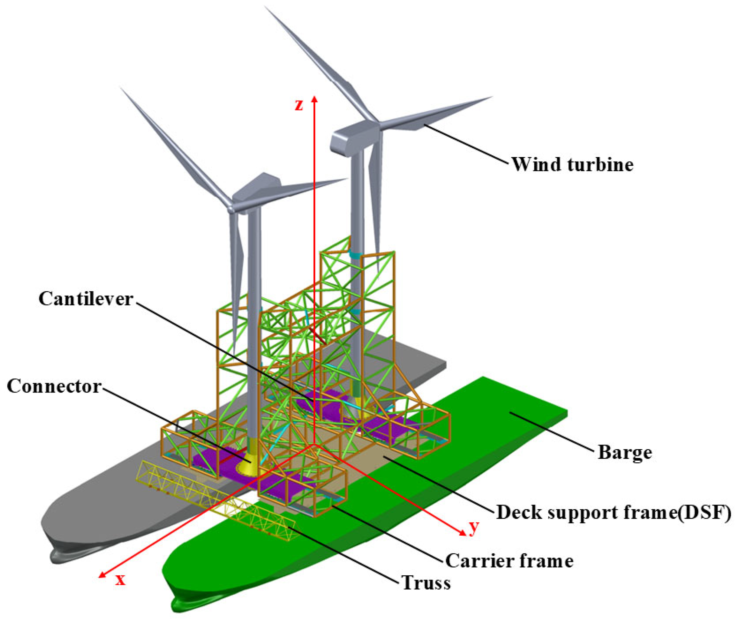
2. Prototype Description
3. Physical Model Description
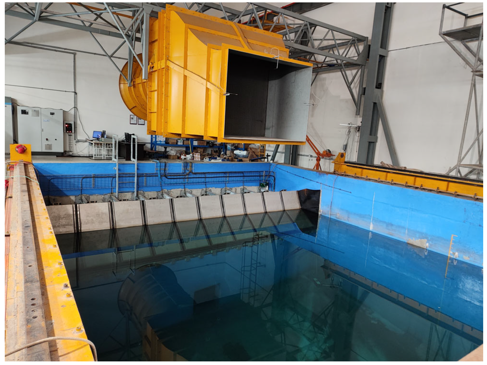
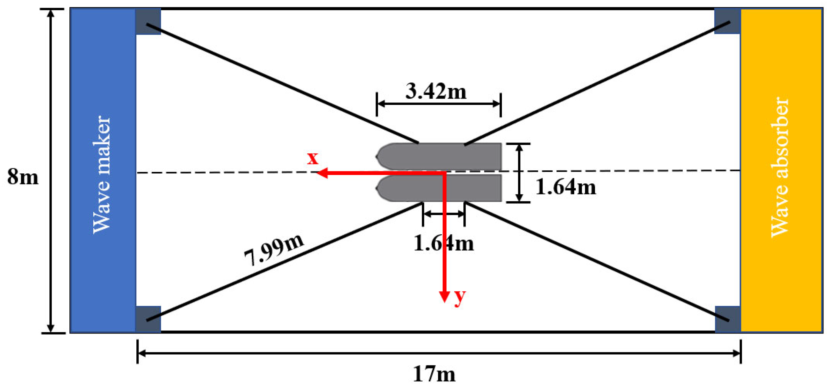
3.1. Ocean Engineering Basin Description
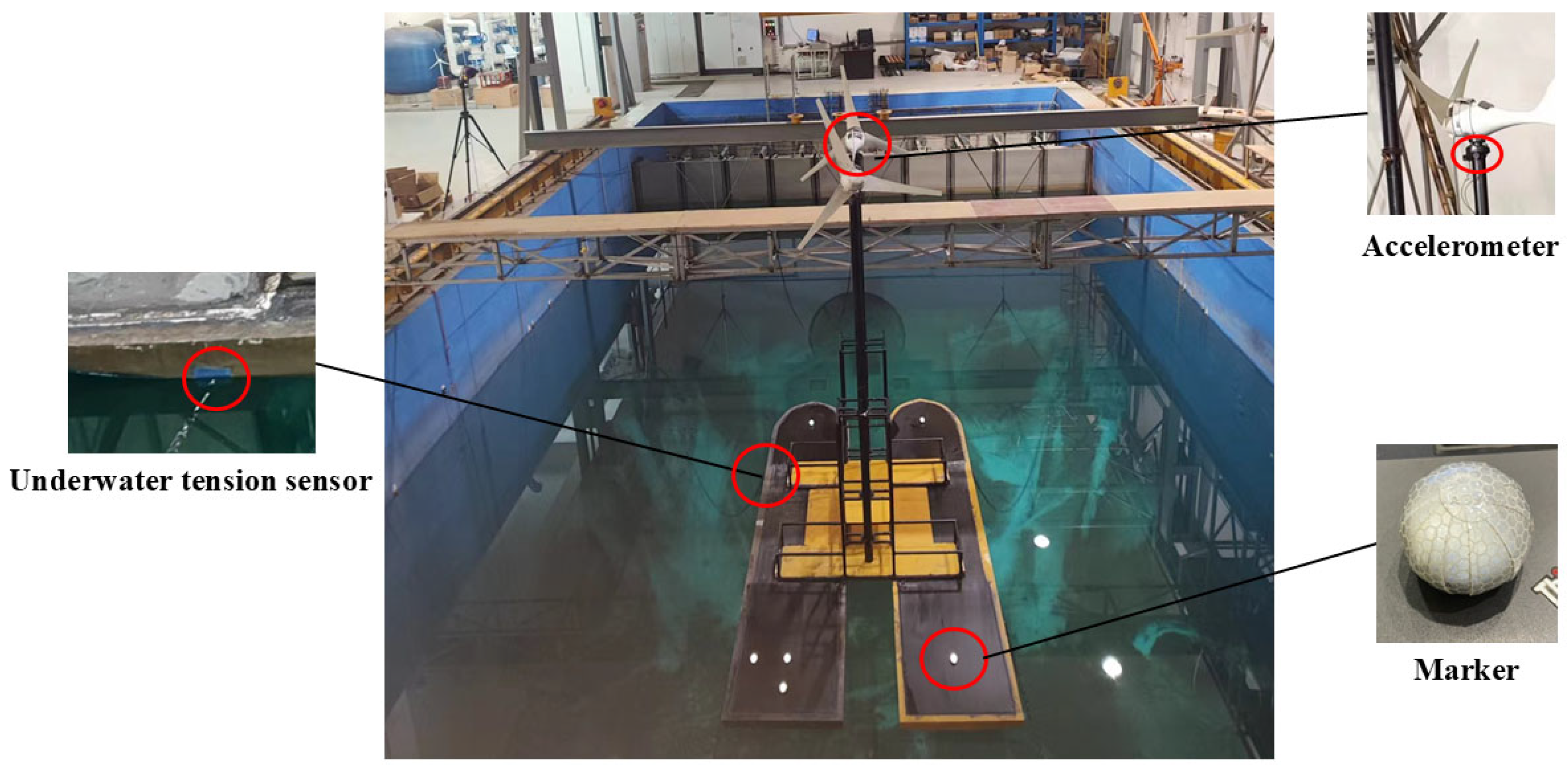
3.2. Physical Model and Test Set-Up Description
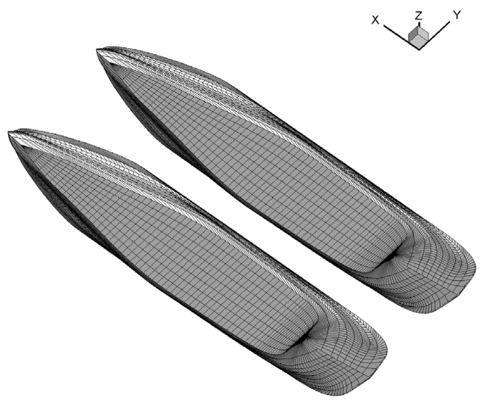
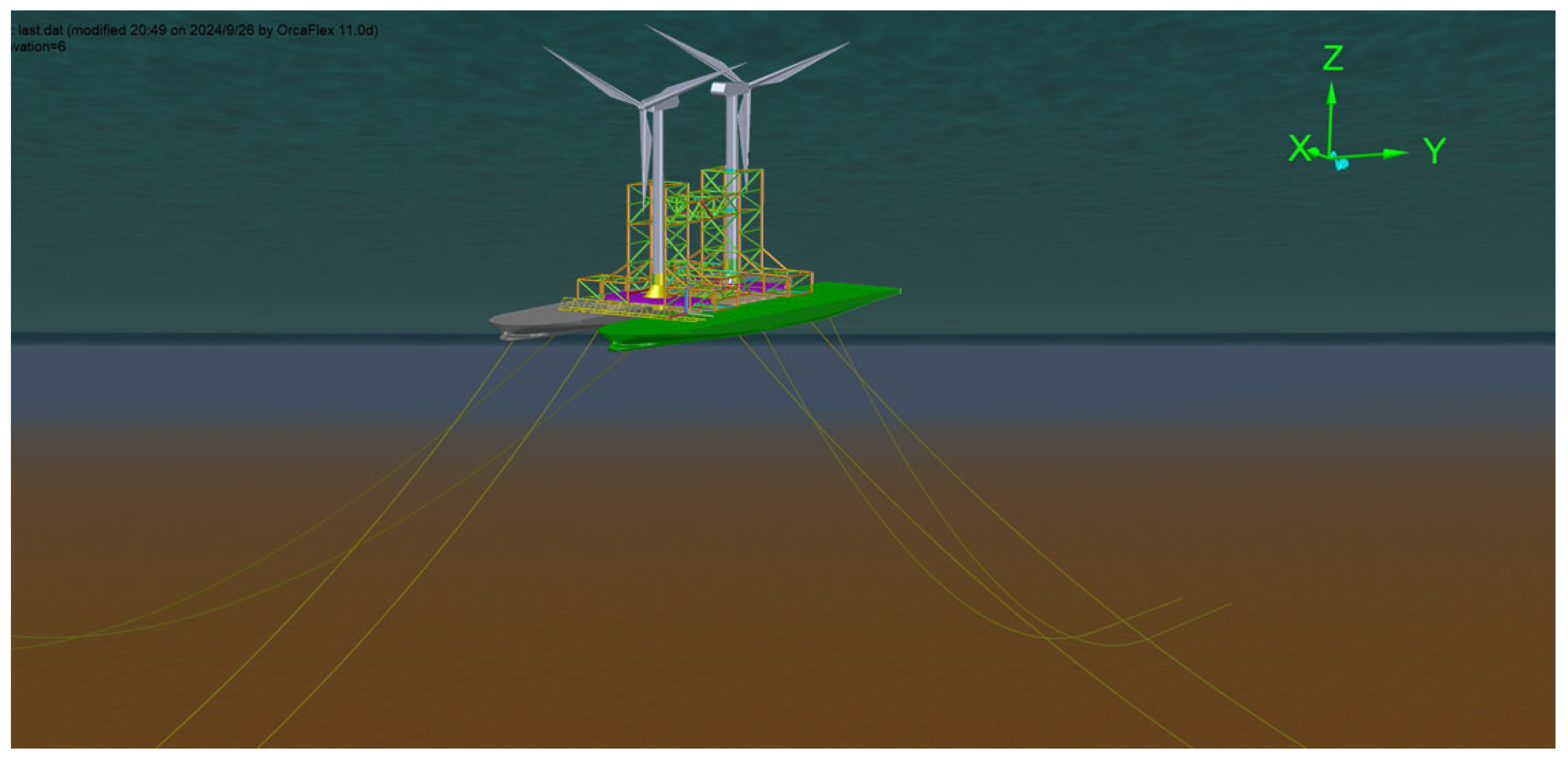
3.2.1. Twin-Barge Model
3.2.2. Topside Module Model
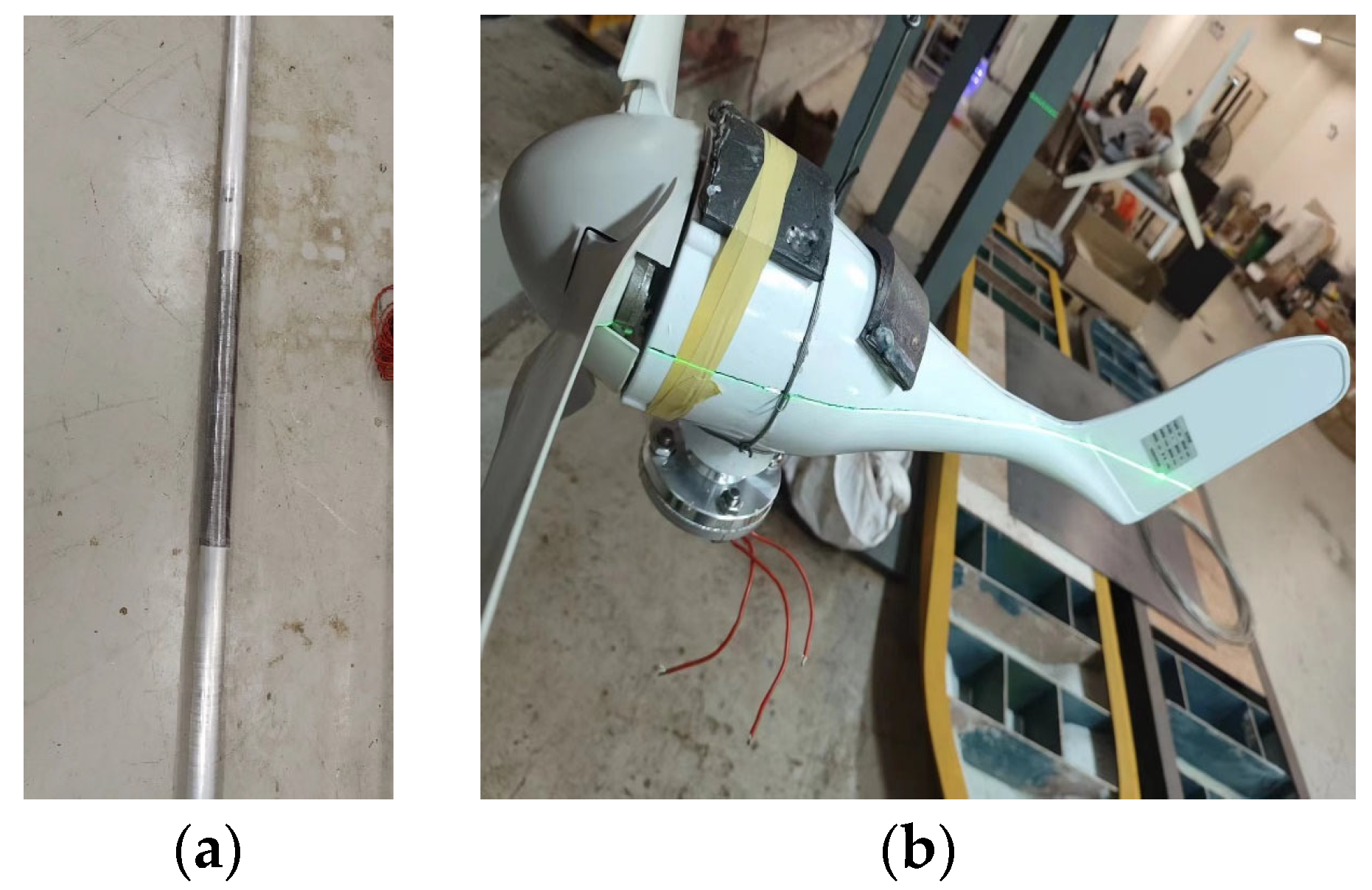
3.2.3. Tower and Wind Turbines Model
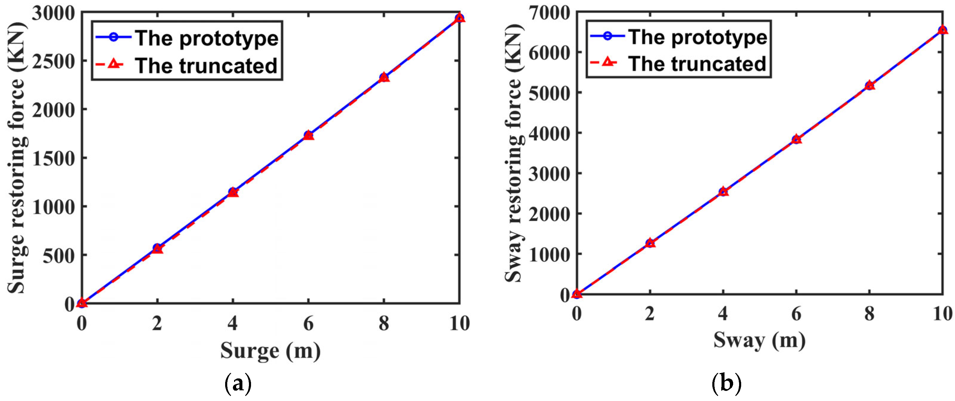
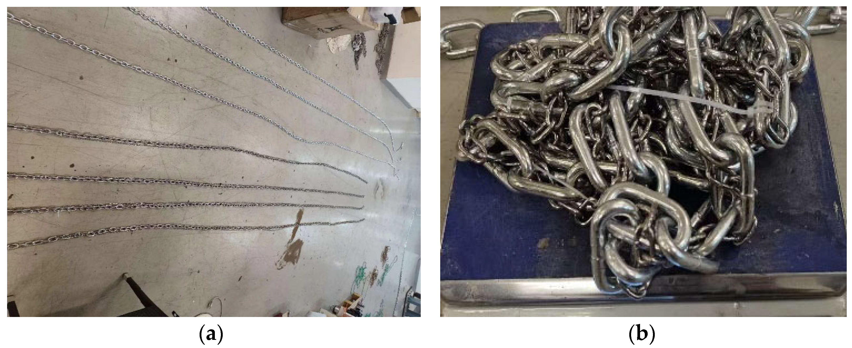
3.2.4. Mooring System Model
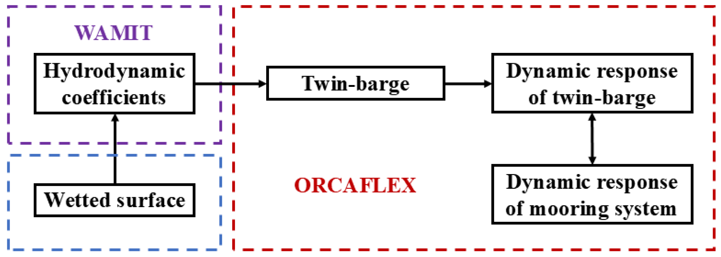
4. Numerical Simulation Methodology
5. Load Cases
6. Preliminary Calibration Experiment
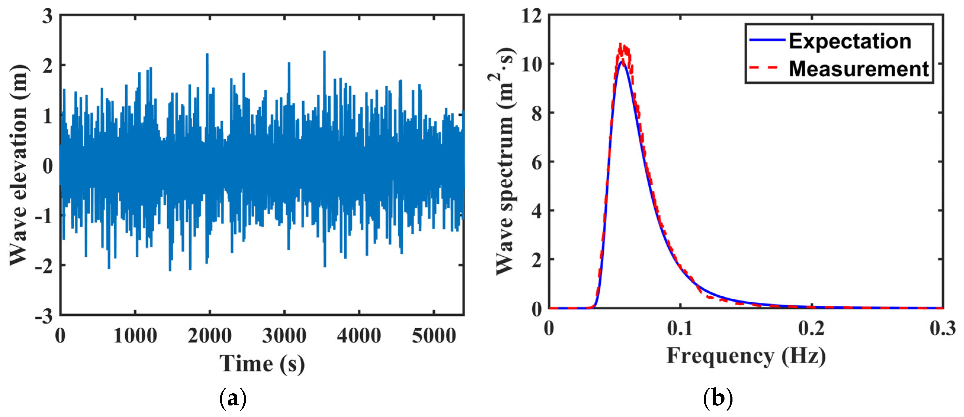
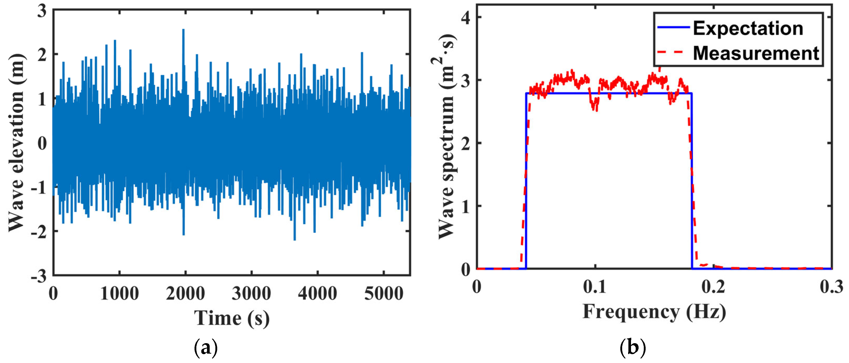
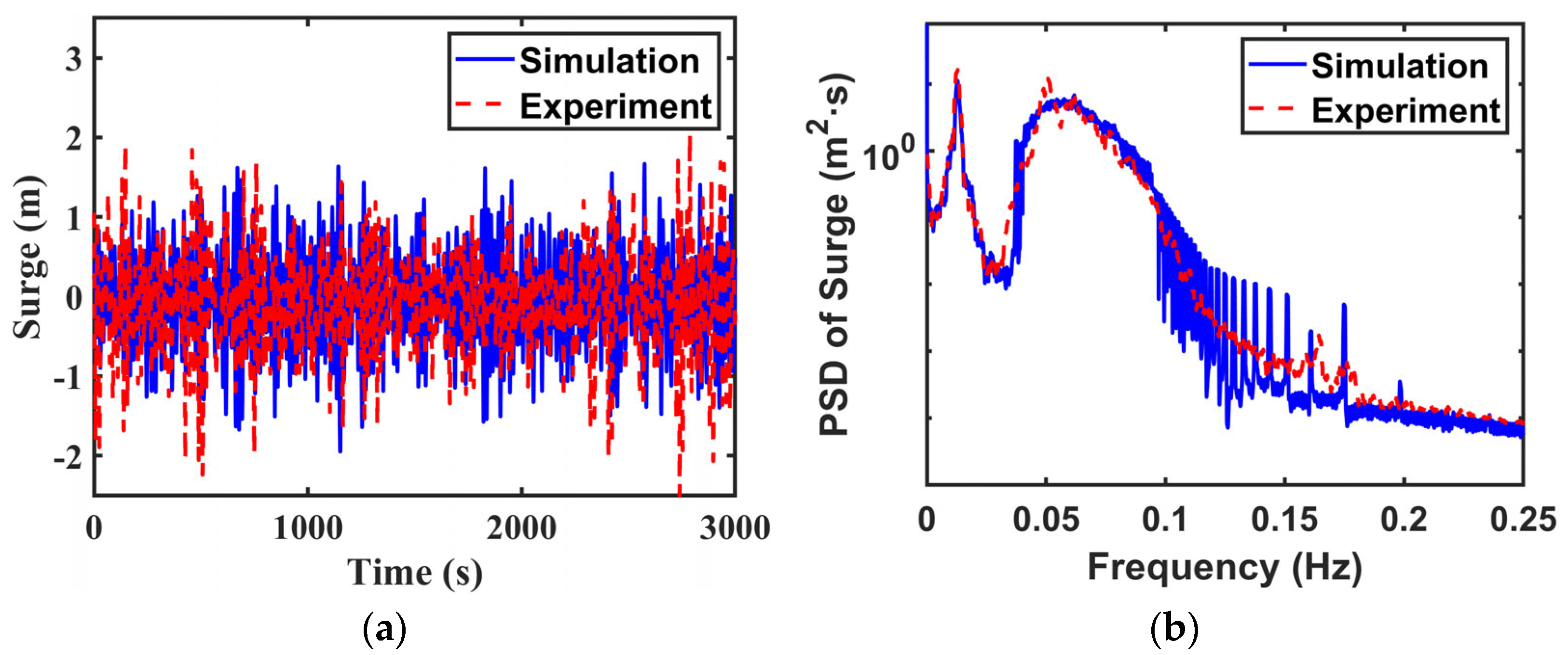
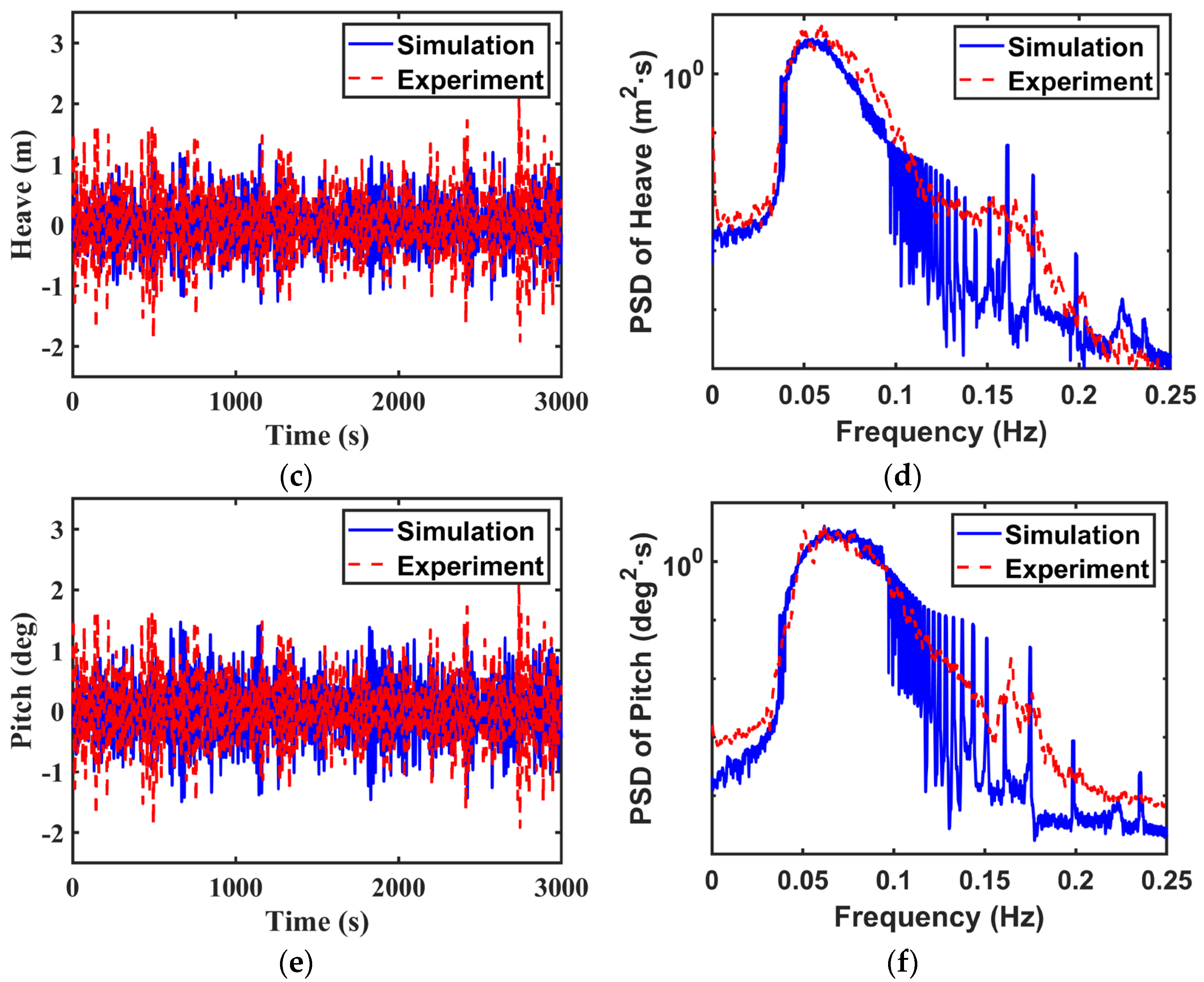
6.1. Validation of Wave Fields
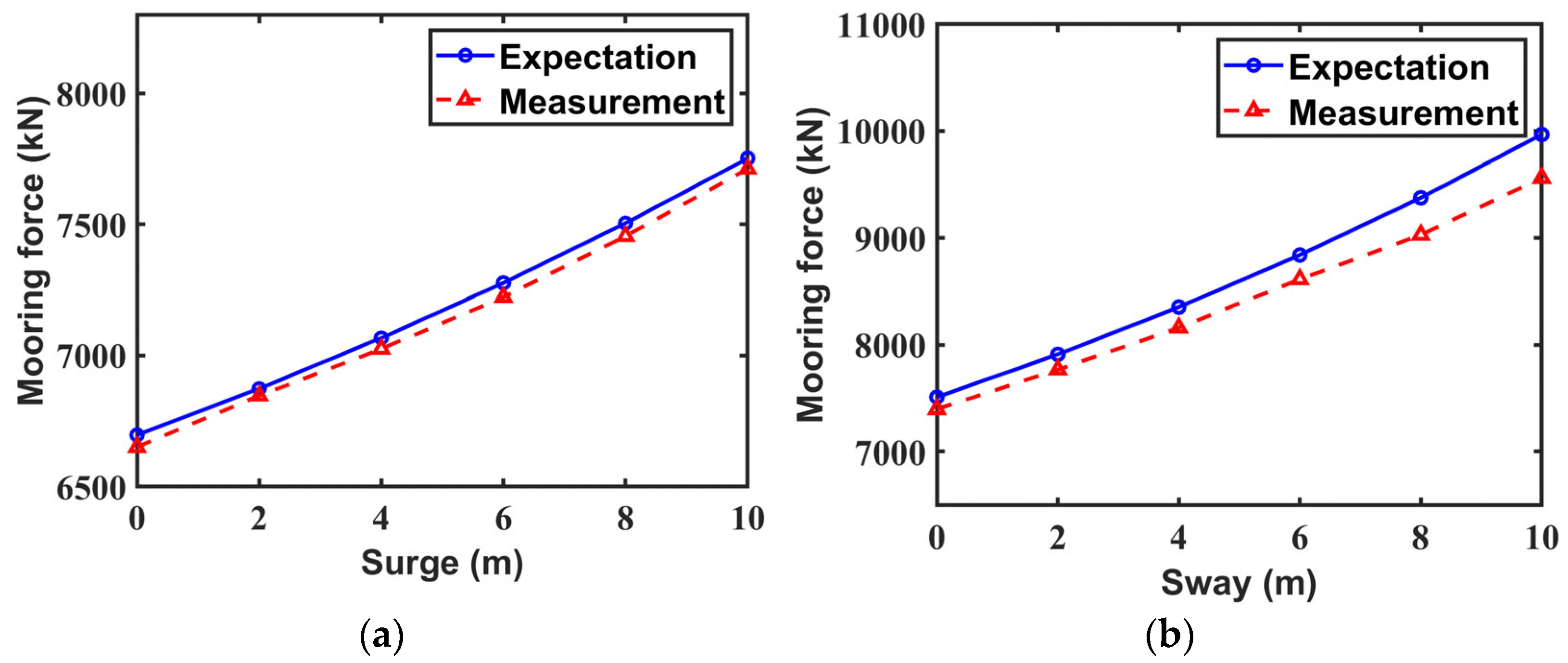
6.2. Validation of Mooring Lines’ Tension
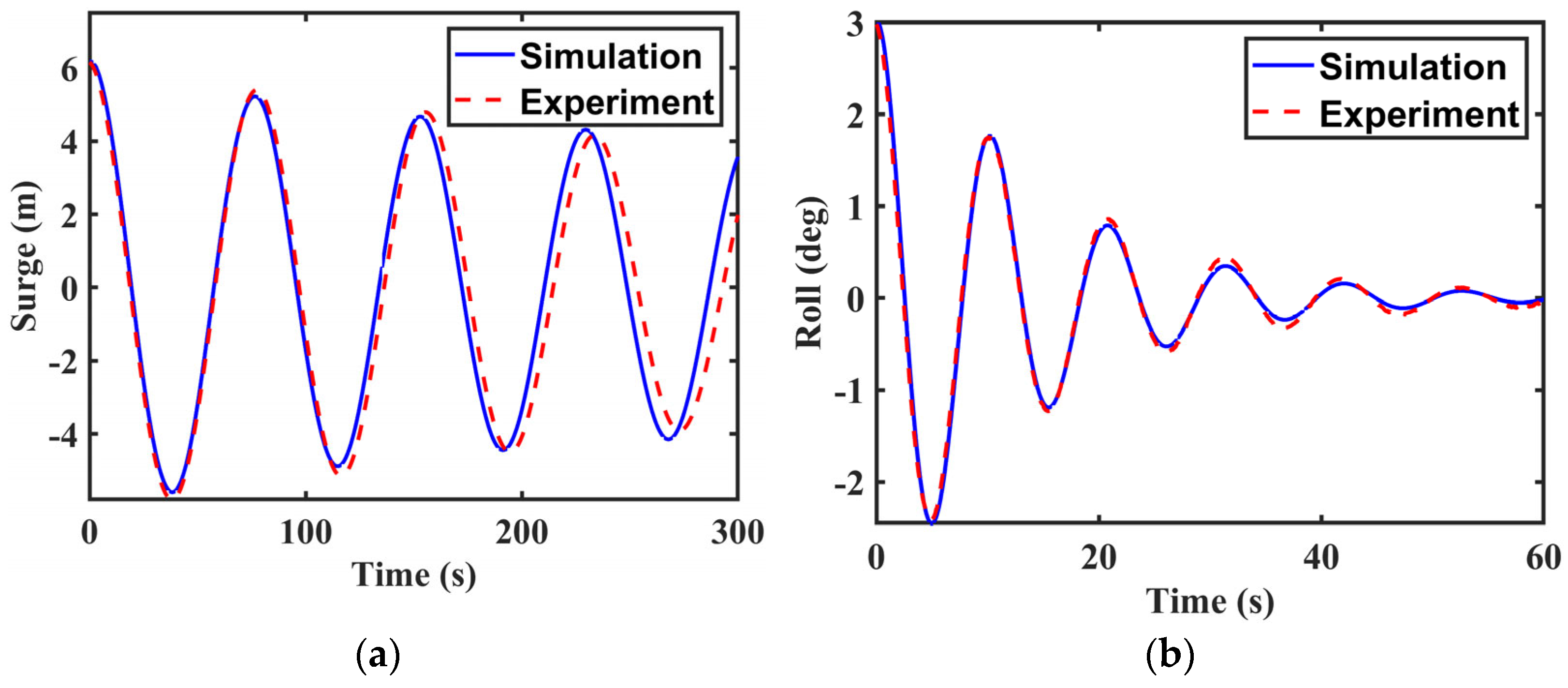
6.3. Free Decay Tests
7. Results and Discussion
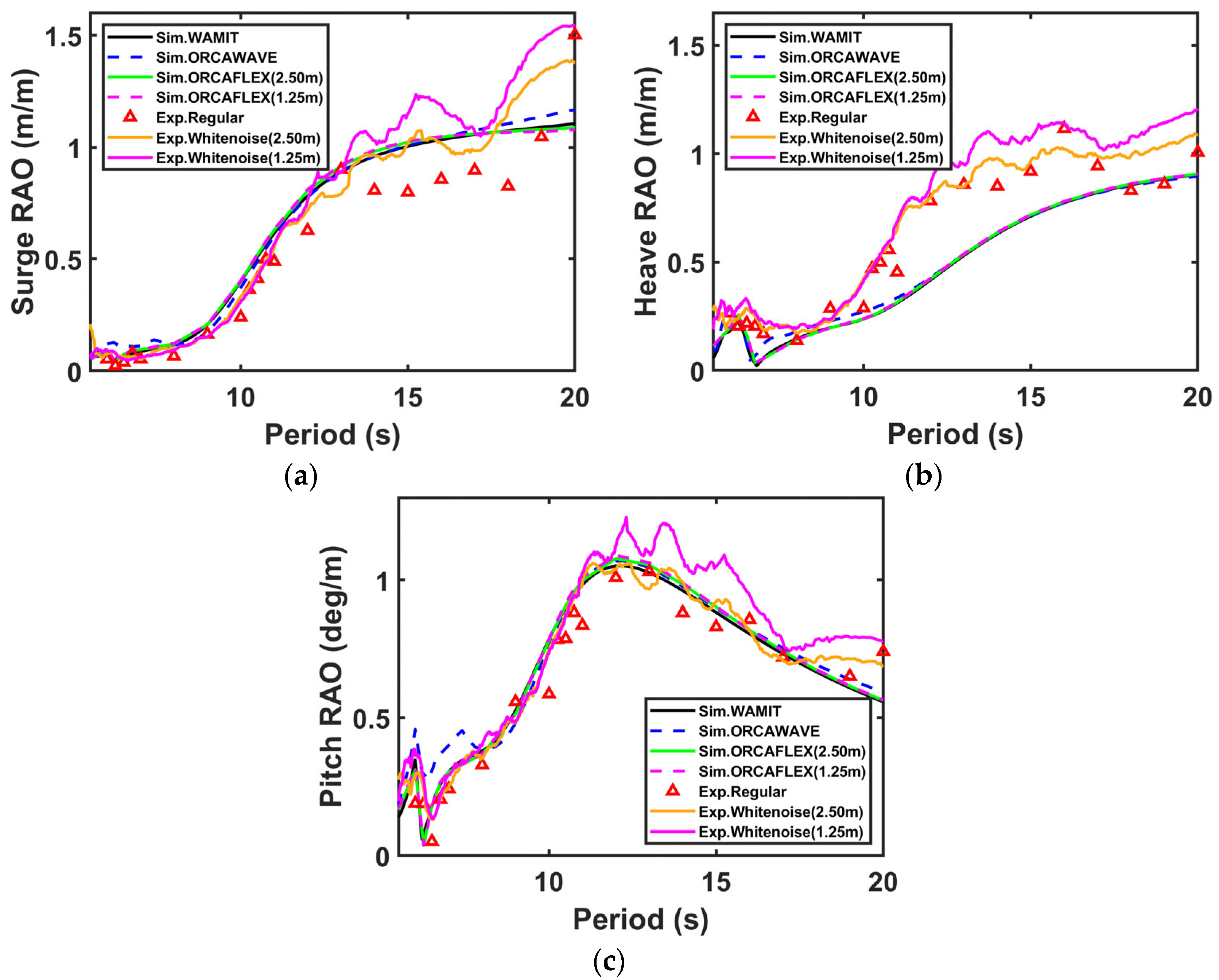
7.1. Motion RAO Tests
7.2. Regular Wave Tests for H = 4.00 m
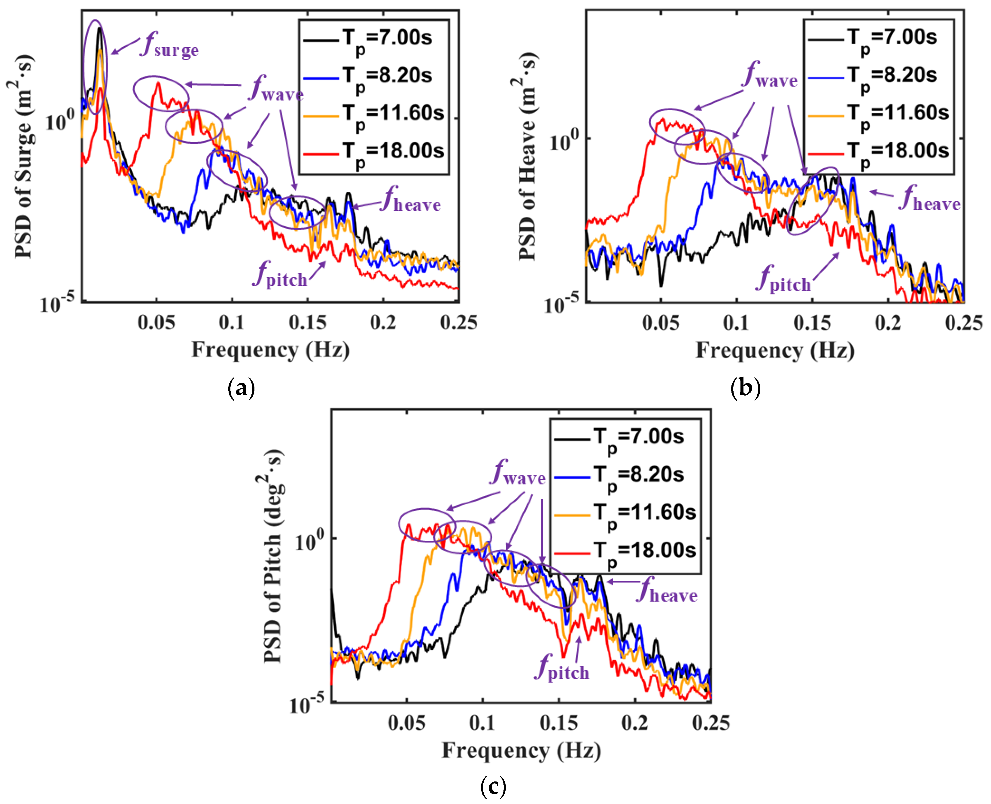
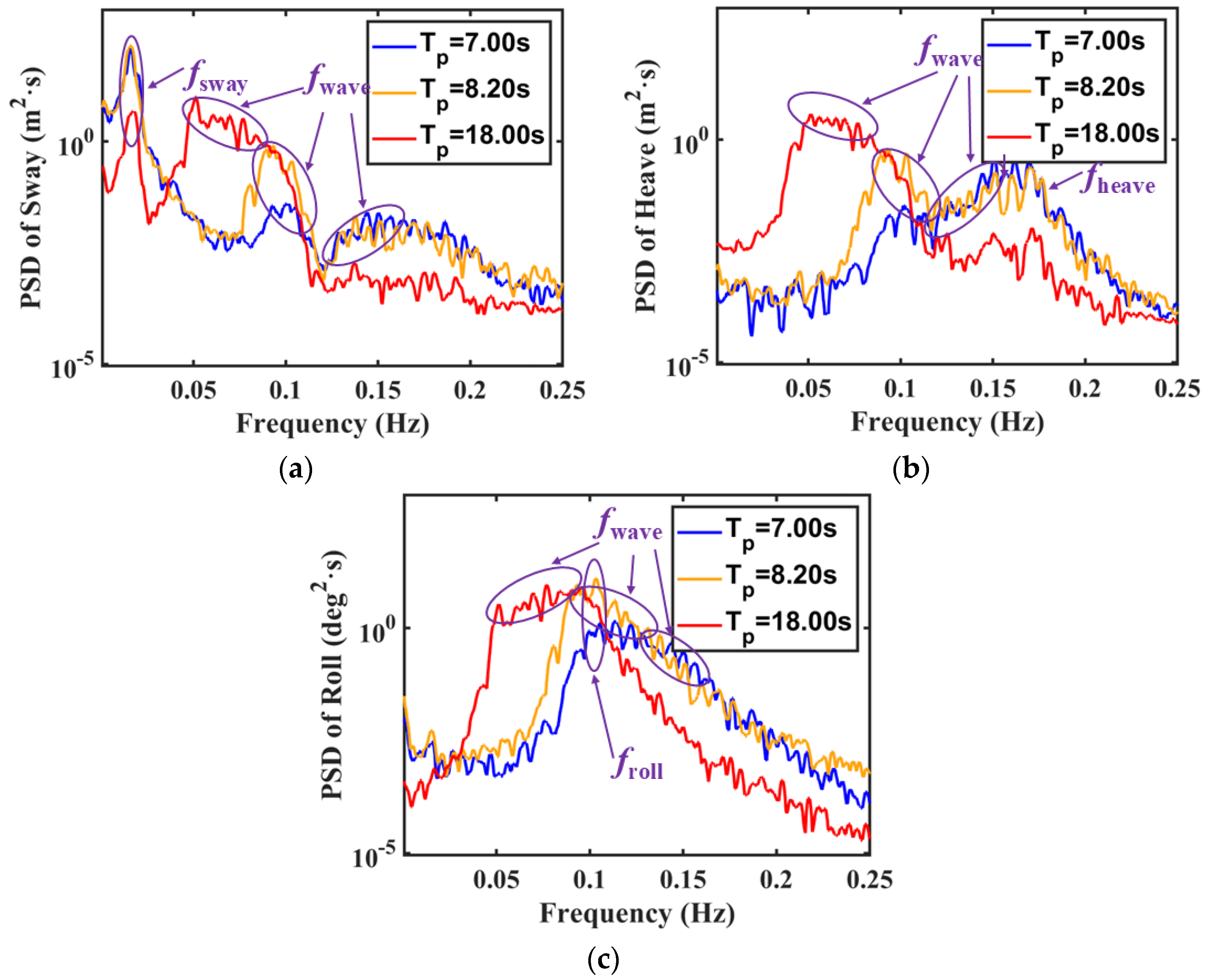
7.3. Random Wave Tests
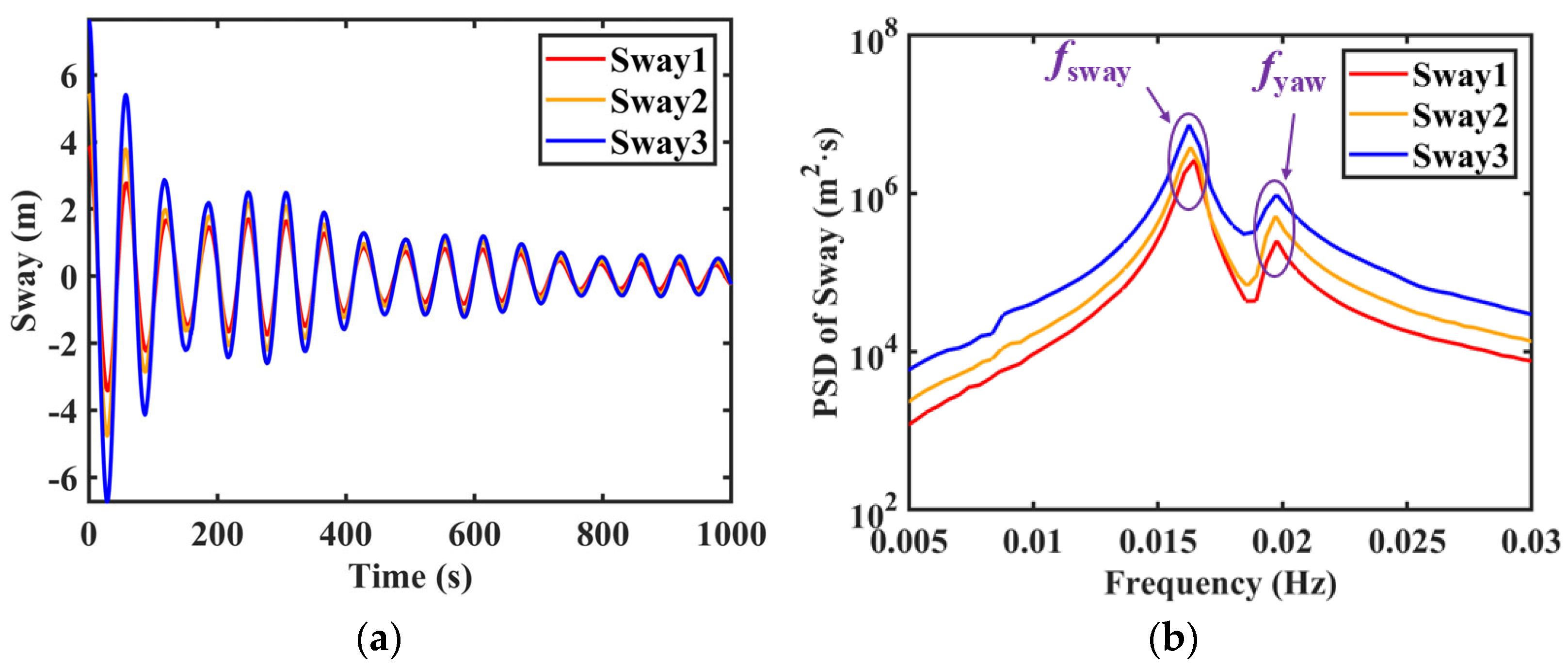
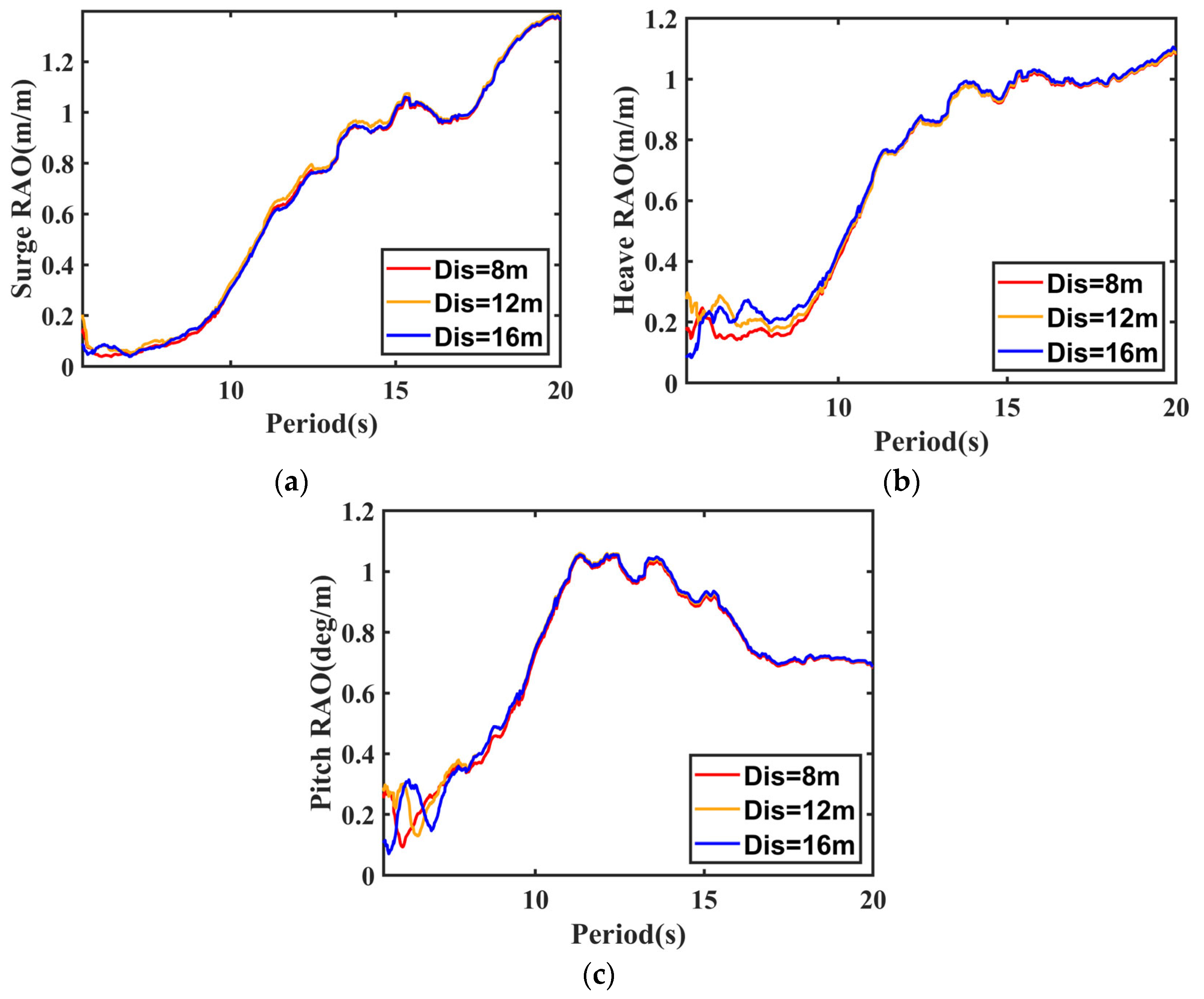
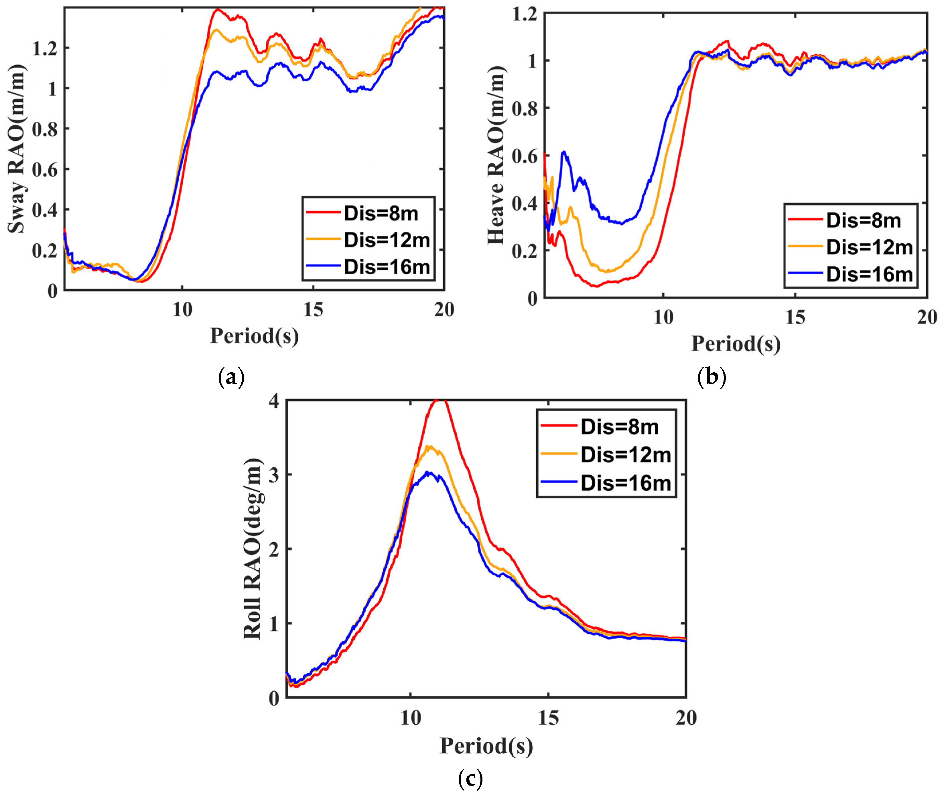
7.4. Influence of the Gap Distance Between Two Barges
8. Motion Prediction
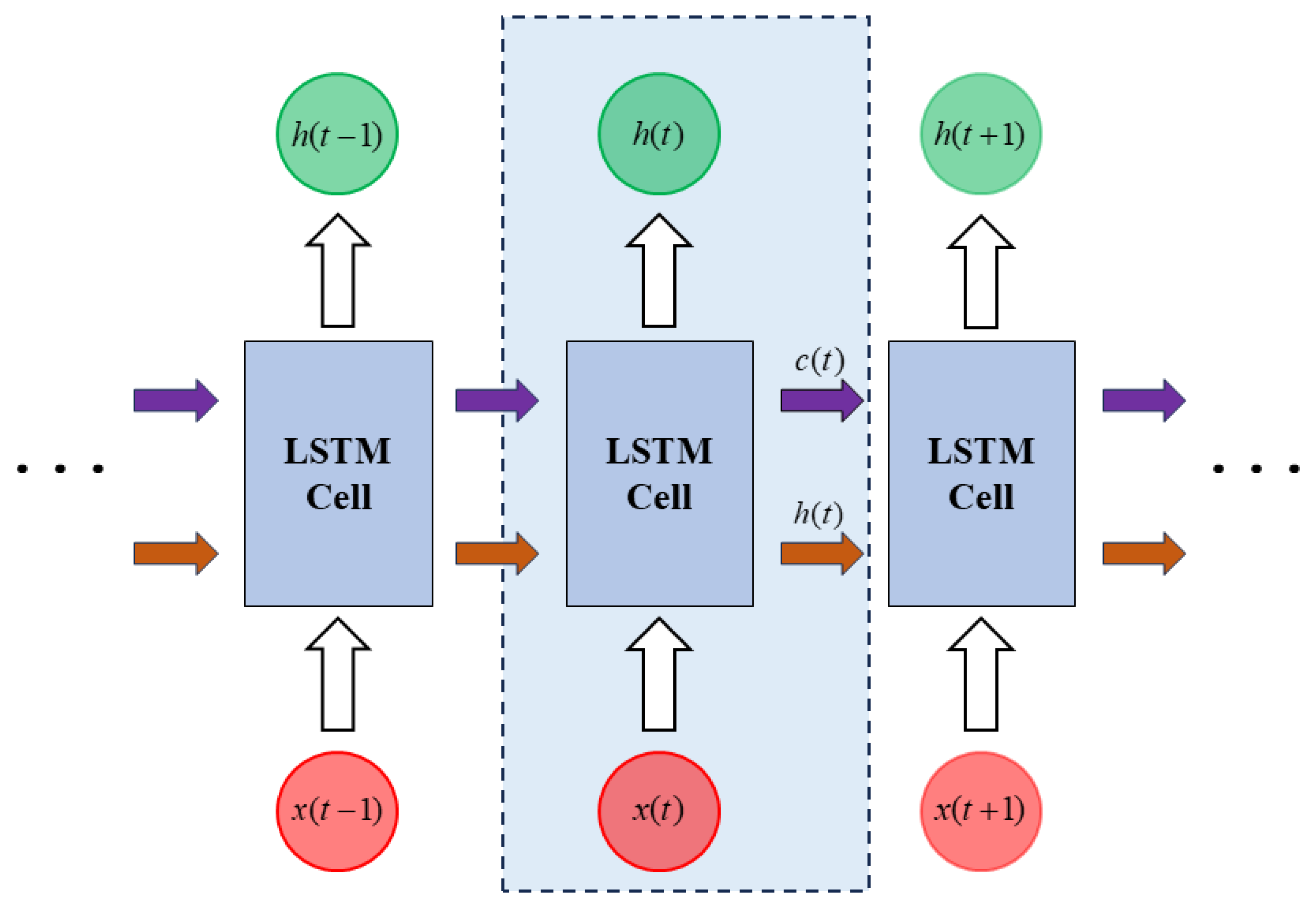
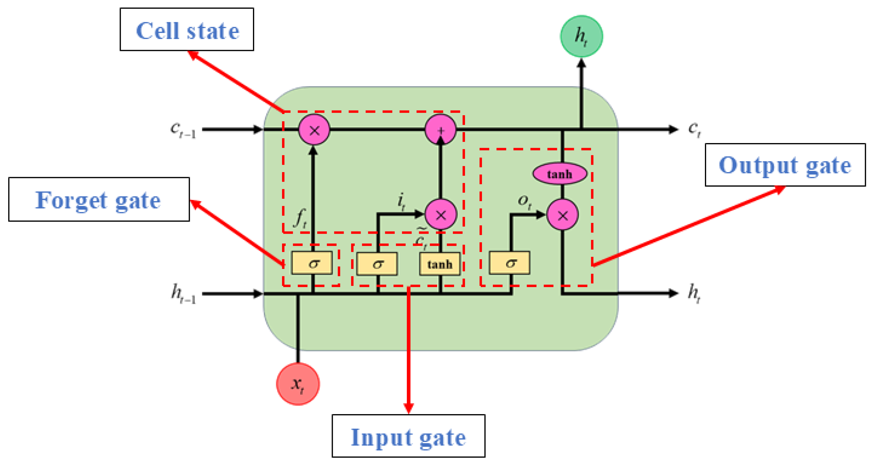
8.1. Introduction to LSTM
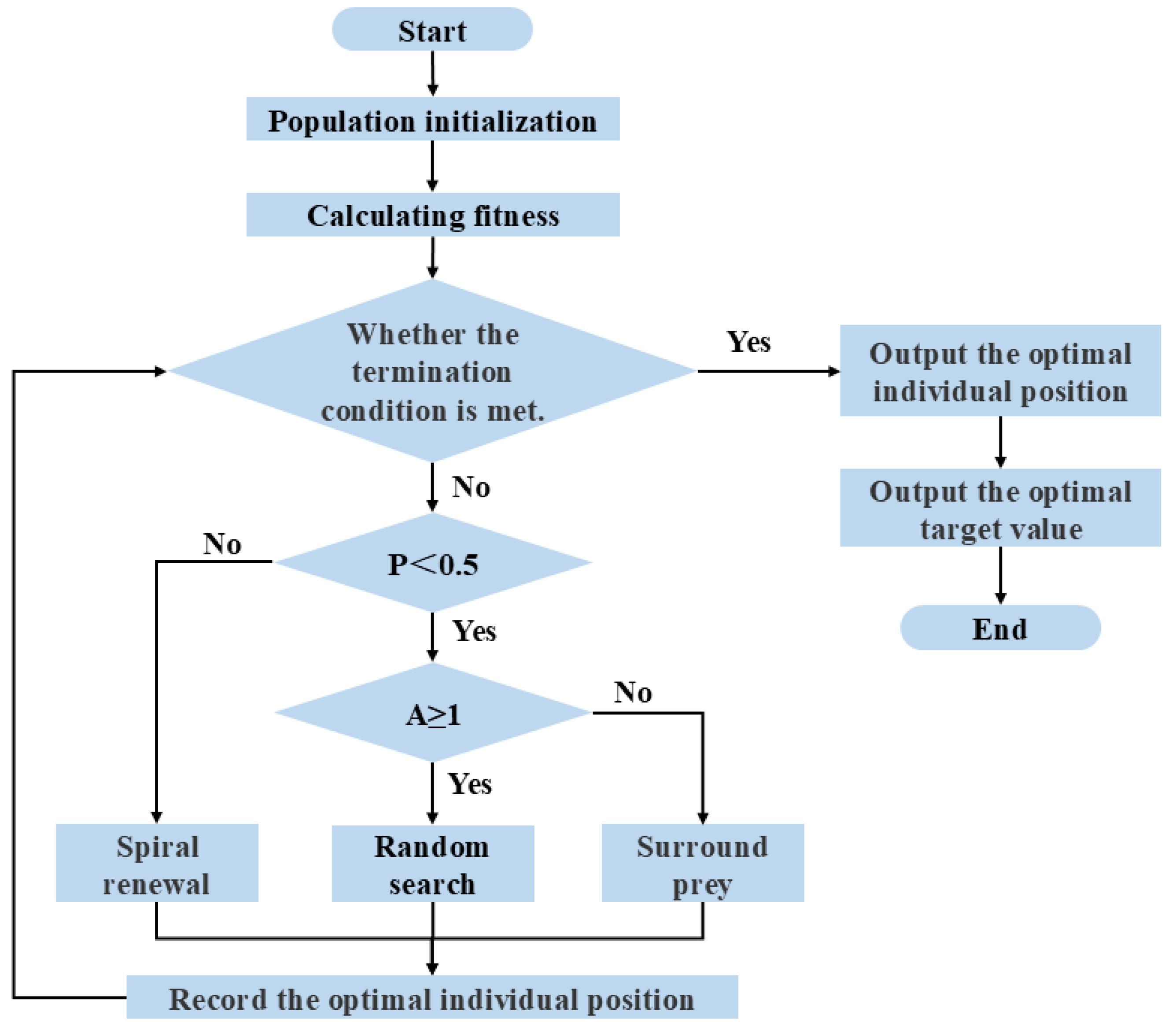
8.2. Introduction to WOA
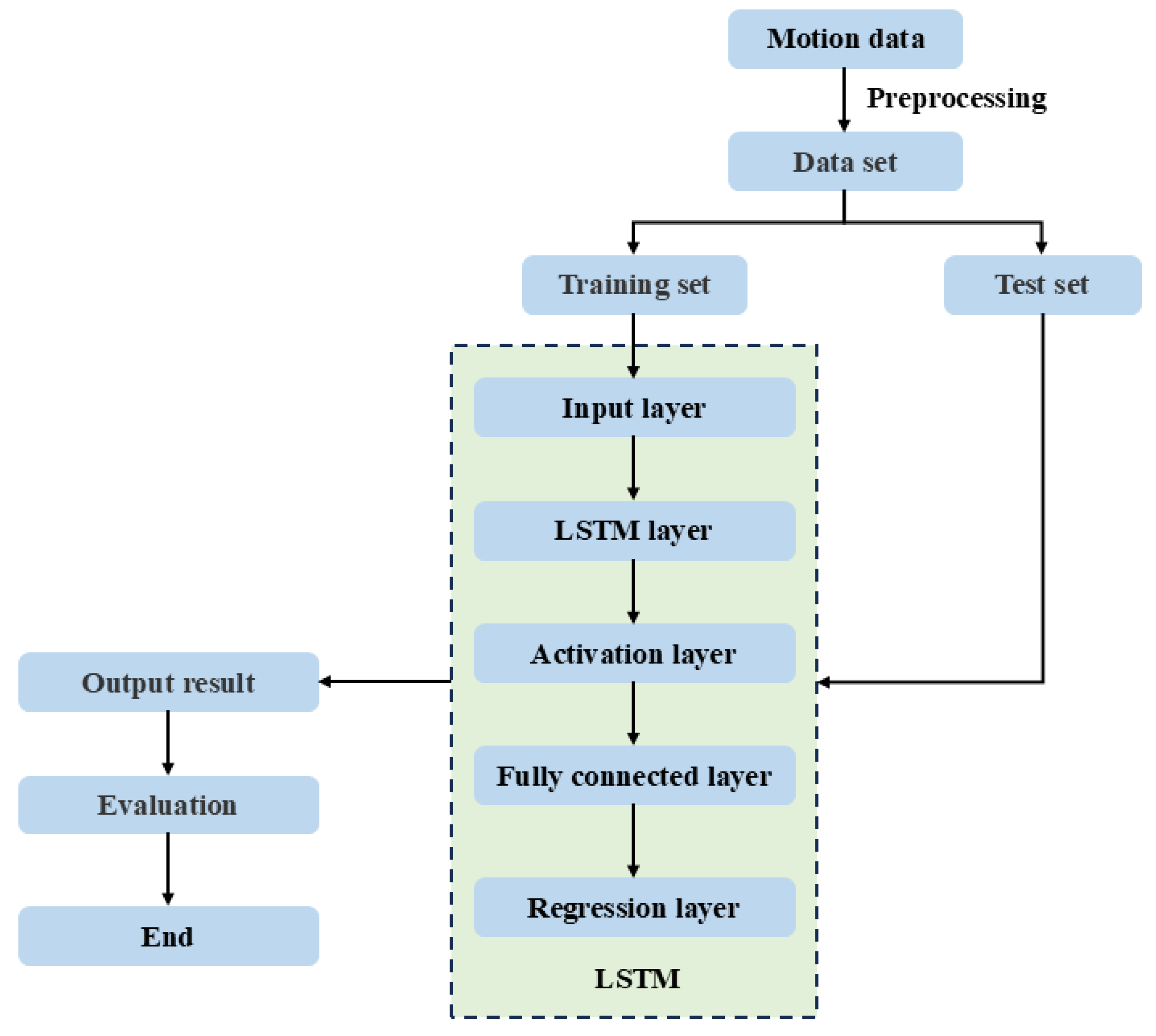
8.3. Model Construction
8.4. Prediction Results
9. Conclusions
Author Contributions
Funding
Data Availability Statement
Conflicts of Interest
References
- Fang, X.; Guo, X.; Tian, X.; Wang, P.; Lu, W.; Li, X. A review on the numerical and experimental modeling of the float-over installations. Ocean Eng. 2023, 272, 113774. [Google Scholar] [CrossRef]
- Qin, L.; Bai, X.; Luo, H.; Li, H.; Ding, H. Review on recent research and technical challenges of float-over installation operation. Ocean Eng. 2022, 253, 111378. [Google Scholar] [CrossRef]
- Edelson, D.; Halkyard, J.; Chen, L.; Chabot, L. Float-over deck installation on spars. In Proceedings of the International Conference on Offshore Mechanics and Arctic Engineering, San Diego, CA, USA, 10–15 June 2007. [Google Scholar]
- Ó’Catháin, M.; Leira, B.J.; Ringwood, J.V.; Gilloteaux, J.-C. A modelling methodology for multi-body systems with application to wave-energy devices. Ocean Eng. 2008, 35, 1381–1387. [Google Scholar] [CrossRef]
- Hu, Z.; Li, X.; Zhao, W.; Wu, X. Nonlinear dynamics and impact load in float-over installation. Appl. Ocean Res. 2017, 65, 60–78. [Google Scholar] [CrossRef]
- Zhu, L.; Zou, M.; Chen, M.; Li, L. Nonlinear dynamic analysis of float-over deck installation for a GBS platform based on a constant parameter time domain model. Ocean Eng. 2021, 235, 109443. [Google Scholar] [CrossRef]
- O’Neill, L.A.; Fakas, E.; Cassidy, M. A novel application of constrained NewWave theory for float-over deck installations. In Proceedings of the International Conference on Offshore Mechanics and Arctic Engineering, Vancouver, BC, Canada, 20–25 June 2004. [Google Scholar]
- Chu, N.; Cochrane, M.; Mobbs, K. Results comparison of computer simulation, model test and offshore installation for Wandoo integrated deck float over installation. In Proceedings of the Offshore Technology Conference, Houston, TX, USA, 4–7 May 1998. [Google Scholar]
- Tahar, A.; Halkyard, J.; Steen, A.; Finn, L. Float over installation method—Comprehensive comparison between numerical and model test results. J. Offshore Mech. Arct. Eng. 2006, 128, 256–262. [Google Scholar] [CrossRef]
- Sun, L.; Taylor, R.E.; Choo, Y.S. Multi-body dynamic analysis of float-over installations. Ocean Eng. 2012, 51, 1–15. [Google Scholar] [CrossRef]
- Ma, Y.; Yuan, L.; Zan, Y.; Zhang, C. Numerical simulation of float-over installation for offshore platform. J. Mar. Sci. Appl. 2018, 17, 79–86. [Google Scholar] [CrossRef]
- Kwak, H.U.; Jung, S.J.; Oh, S.H. Assessment of docking operation during float-over installation on jacket structure. In Proceedings of the ISOPE International Ocean and Polar Engineering Conference, Sapporo, Japan, 10–15 June 2018. [Google Scholar]
- Xiong, G.; Liang, F.S.; Li, X. Numerical analysis and risk study of transportation and float-over installation of large offshore converter stations. Mar. Eng. Equip. Technol. 2023, 10, 1–12. [Google Scholar]
- Du, S.K.; Fan, J. Study on hydrodynamic interaction of multi-body in offshore float-over installation. China Shipbuild. 2022, 63, 57–68. [Google Scholar]
- Choi, Y.R.; Hong, S.Y. An analysis of hydrodynamic interaction of floating multi-body using higher-order boundary element method. In Proceedings of the ISOPE International Ocean and Polar Engineering Conference, Kitakyushu, Japan, 26–31 May 2002. [Google Scholar]
- Xu, L.; Yang, J.; Li, X. Study on hydrodynamic performance and wave elevation of twin-barge system. China Shipbuild. 2012, 53, 217–226. [Google Scholar]
- Wang, S.F. Multibody Dynamic Analysis of the Lift-Off Operation: A Time Domain Approach. Master’s Thesis, Delft University of Technology, Delft, The Netherlands, 5 June 2015. [Google Scholar]
- Li, B. Multi-body hydrodynamic resonance and shielding effect of vessels parallel and nonparallel side-by-side. Ocean Eng. 2020, 218, 108188. [Google Scholar] [CrossRef]
- Li, H.; Li, X.; Zhang, W. Hydrodynamics of a three-vessel system in twin-vessel float-over method. J. Mar. Platf. 2021, 2, 46–51. [Google Scholar]
- Zhang, W.; Li, H. Numerical simulation of hydrodynamic response for three-vessel float-over operations. Ship Electr. Technol. 2023, 43, 77–80. [Google Scholar]
- Koo, B.; Magee, A.; Lambrakos, K. Model tests for float-over installation of spar topsides. In Proceedings of the 29th International Conference on Offshore Mechanics and Arctic Engineering, Shanghai, China, 6–11 June 2010. [Google Scholar]
- Kurian, V.J.; Baharuddin, N.H.; Magee, A. Model tests for dynamic responses of float-over barge in shallow wave basin. In Proceedings of the ISOPE International Ocean and Polar Engineering Conference, Anchorage, AK, USA, 30 June–5 July 2013. [Google Scholar]
- Magee, A.; Yunos, N.Z.M.; Kurian, V.J. Model testing capabilities for verification of float-over operations. In Proceedings of the ISOPE International Ocean and Polar Engineering Conference, Busan, Republic of Korea, 15–20 June 2014. [Google Scholar]
- Xiong, L.; Lu, H.; Yang, J.; Zhang, W.; Yang, G. Experimental investigation on global responses of a large float-over barge in extremely shallow water. In Proceedings of the ISOPE International Ocean and Polar Engineering Conference, Kona, HI, USA, 21–26 June 2015. [Google Scholar]
- Dessi, D.; Faiella, E.; Pigna, C.; Celli, C.; Miliante, T.; Di Paolo, E. Experimental analysis of topside transportation with a double-barge float-over system. In Proceedings of the ISOPE International Ocean and Polar Engineering Conference, San Francisco, CA, USA, 25–30 June 2017. [Google Scholar]
- Dessi, D.; Faiella, E.; Saltari, F. Experimental analysis of the station keeping response of a double-barge float-over system with an elastically scaled physical model. In Proceedings of the ISOPE International Ocean and Polar Engineering Conference, San Francisco, CA, USA, 25–30 June 2017. [Google Scholar]
- Xu, X. Coupled Dynamic Response Research of Float-over Installation System. Ph.D. Thesis, Shanghai Jiao Tong University, Shanghai, China, 2016. [Google Scholar]
- Wang, B.; Qin, L.C.; Wang, L. Model Tests of Dynamic Positioning Float-over Installation Method in Offloading Conditions. Lab. Res. Explor. 2017, 36, 12. [Google Scholar]
- Yang, G.; Lü, H.; Xiong, L.; Yang, N. Analysis of motion characteristics and grounding conditions of large float-over installation barges in extremely shallow water. J. Ship Mech. 2018, 22, 827–837. [Google Scholar]
- Jin, X.; Wang, A.M.; Li, H.; Yu, W.; He, M.; Wang, A. Float-over installation technology with a DP2 class dynamic-positioning semisubmersible vessel. In Proceedings of the ISOPE International Ocean and Polar Engineering Conference, Sapporo, Japan, 10–15 June 2018. [Google Scholar]
- Kim, N.W.; Nam, B.W.; Kwon, Y.J.; Park, I.B.; Cho, S.K.; Sung, H.G. An experimental study on the float-over installation of a semi-submersible. In Proceedings of the ISOPE International Ocean and Polar Engineering Conference, Honolulu, HI, USA, 16–21 June 2019. [Google Scholar]
- Luo, H.; Wang, J.; Bai, X.; Li, H.; Qin, L.; Zhu, S. Research on step-by-step experiments and numerical simulation of float-over installation based on rapid load transfer technology. China Shipbuild. 2020, 61, 173–185. [Google Scholar]
- Bai, X.; Luo, H.; Xie, P. Experimental analysis of hydrodynamic response of the twin-barge floatover installation for mega topsides. Ocean Eng. 2021, 219, 108302. [Google Scholar] [CrossRef]
- Tao, W.; Wang, S.; Song, X.; Li, H. Experimental investigation on continuous load transfer process of twin-barge float-over installation. Ocean Eng. 2021, 234, 109309. [Google Scholar] [CrossRef]
- He, H.; Wang, L.; Zhu, Y.; Xu, S. Numerical and experimental study on the docking of a dynamically positioned barge in float-over installation. Ships Offshore Struct. 2021, 16, 505–515. [Google Scholar] [CrossRef]
- Li, X.; Ruan, Z. Numerical simulation and water tank tests of short-distance transportation of large platform twin-barge float-over installation. China Offshore Platf. 2023, 38, 61–69. [Google Scholar]
- Barooni, M.; Ghaderpour Taleghani, S.; Bahrami, M.; Sedigh, P.; Sogut, D.V. Machine learning-based forecasting of metocean data for offshore engineering applications. Atmosphere 2024, 15, 640. [Google Scholar] [CrossRef]
- Lei, Y.; Zheng, X.Y.; Li, W.; Zheng, H.D.; Zhang, Q.; Zhao, S.X.; Cai, X.; Ci, X.; He, Q. Experimental study of the state-of-the-art offshore system integrating a floating offshore wind turbine with a steel fish farming cage. Mar. Struct. 2021, 80, 103076. [Google Scholar] [CrossRef]
- Zheng, H.D.; Zheng, X.Y.; Lei, Y.; Li, D.-A.; Ci, X. Experimental validation on the dynamic response of a novel floater uniting a vertical-axis wind turbine with a steel fishing cage. Ocean Eng. 2022, 243, 110257. [Google Scholar] [CrossRef]
- Ci, X.; Li, W.; Lei, Y.; Gao, S.; Zhang, S.; Zheng, X.Y. Experimental study on the dynamic responses of a 2 MW cross-shaped multi-column spar floating offshore wind turbine. In Proceedings of the International Conference on Environment Sciences and Renewable Energy; Springer Nature Singapore: Singapore, 2022; pp. 137–149. [Google Scholar]
- Molins, C.; Trubat, P.; Gironella, X.; Campos, A. Design Optimization for a Truncated Catenary Mooring System for Scale Model Test. J. Mar. Sci. Eng. 2015, 3, 1362–1381. [Google Scholar] [CrossRef]
- Lee, C.H.; Newman, J.N. WAMIT User Manual; WAMIT, Inc.: Chestnut Hill, MA, USA, 2006; p. 42. [Google Scholar]
- Orcina, Ltd. Orcaflex User Manual: Orcaflex Version 10.3c; Orcina, Ltd.: Cumbria, UK, 2018. [Google Scholar]
- DNVGL-OS-E301; Offshore Standard: Position Mooring. DNV GL AS: Oslo, Norway, 2015.
- SNAME T&R 5-5A; Guidelines for Site Specific Assessment of Mobile Jack-Up Units. SNAME: Jersey City, NJ, USA, 2008.
- Chandrasekaran, S.; Sri Charan, V.V.S. Time-domain analysis of a bean-shaped multi-body floating wave energy converter with a hydraulic power take-off using WEC-Sim. Energy 2021, 223, 119985. [Google Scholar]
- GB/T 42176-2022; The Grade of Wave Height. State Administration for Market Regulation: Beijing, China, 2022.
- Zhao, W.; Pan, Z.; Lin, F.; Li, B.; Taylor, P.H.; Efthymiou, M. Estimation of gap resonance relevant to side-by-side offloading. Ocean Eng. 2018, 153, 1–9. [Google Scholar] [CrossRef]
- Huang, X.; Xiao, W.; Yao, X.; Gu, J.; Jiang, Z. An experimental investigation of reduction effect of damping devices in the rectangular moonpool. Ocean Eng. 2020, 196, 106767. [Google Scholar] [CrossRef]


| Parameters | Values |
|---|---|
| Length overall of a single barge (m) | 171 |
| Molded breadth of a single barge (m) | 35 |
| Molded depth of a single barge (m) | 9 |
| Draft (m) | 4.66 |
| Water depth (m) 1 | 250 |
| Mass of a single barge (t) | 11,161.21 |
| Displacement of twin barge (t) | 39,141.29 |
| Center of gravity of twin barge (m) | (0.21, 0, 15.97) |
| Roll moment of inertia about the CG of twin barge (kg·m2) | 7.98 × 10¹⁰ |
| Pitch moment of inertia about the CG of twin barge (kg·m2) | 1.11 × 10¹¹ |
| Yaw moment of inertia about the CG of twin barge (kg·m2) | 6.34 × 10¹⁰ |
| Parameters | Line 1,2,3,4 | Line 5,6,7,8 |
|---|---|---|
| Type | Studless chain R4 | Studless chain R4 |
| Diameter (mm) | 157 | 180 |
| Equivalent diameter (mm) | 283 | 324 |
| Break load (kN) | 21,234 | 26,278 |
| Mass density (kg/m) | 493 | 648 |
| Axis stiffness (kN) | 1.96 × 10⁶ | 2.55 × 10⁶ |
| Length (m) | 775 | 880 |
| Mooring radius (m) | 786 | 862 |
| Depth of fairleads below SWL (m) | 0.66 | 0.66 |
| Distance between fairleads and axis z (m) | 89 | 54 |
| Scale Factor (Prototype/Model) | |
|---|---|
| Linear dimension | λ |
| Linear velocity | λ1/2 |
| Linear acceleration | 1 |
| Time or period | λ1/2 |
| Angle | 1 |
| Mass 2 | γλ3 |
| Displacement volume | γλ3 |
| Force | γλ3 |
| Moment | γλ4 |
| Moment of inertia | γλ5 |
| Type | Capacity | Resolution | |
|---|---|---|---|
| Wave probe | JM5900 | ±500 mm | 0.02 mm |
| Accelerometer | AI050 | 10 g | 0.0001 g |
| Underwater tension sensor | LA1 | 300 N | 0.05 N |
| 6-DOF motion capture system | Qualisys 700+ | - | 0.1 mm |
| Full Scale | 1:50 Scale (Target) | 1:50 Scale (Achieved) | Deviation | |
|---|---|---|---|---|
| Length overall (m) | 171 | 3.42 | 3.42 | 0 |
| Molded breadth (m) | 35 | 0.70 | 0.70 | 0 |
| Molded depth (m) | 9 | 0.18 | 0.18 | 0 |
| Mass of black barge (kg) | 11,161,210 | 87.11 | 87.39 | +0.31% |
| Mass of yellow barge (kg) | 11,161,210 | 87.11 | 87.76 | +0.75% |
| Center of gravity of black barge (m) | 6.40 | 0.13 | 0.13 | −1.93% |
| Center of gravity of yellow barge (m) | 6.40 | 0.13 | 0.13 | −2.00% |
| Size (mm) | Material | Mass (kg) | Center of Gravity (m) | |
|---|---|---|---|---|
| Truss carriage frame (OD × ID) | 22 × 18 | Aluminum alloy | 12.721 | 0.406 |
| Deck support frame | 1324 × 952 × 4 | Steel | 39.578 | 0.002 |
| Cantilever beams | 1260 × 310 × 3 | Steel | 9.132 | 0.028 |
| Ballast (L × B × H) | 678 × 318 × 8 722 × 362 × 2 | Steel | 17.613 | 0.223 |
| Parameters | Full Scale | 1:50 Scale (Target) | 1:50 Scale (Achieved) | Deviation |
|---|---|---|---|---|
| Mass of wind turbine1 (kg) | 900,000 | 7.02 | 7.00 | −0.30% |
| Mass of wind turbine2 (kg) | 900,000 | 7.02 | 6.98 | −0.60% |
| Center of gravity of wind turbine (m) | 143 | 2.86 | 2.86 | 0 |
| Mass of tower1 (kg) | 1,650,000 | 12.88 | 12.92 | +0.30% |
| Mass of tower2 (kg) | 1,650,000 | 12.88 | 12.94 | 0.05% |
| Center of gravity of tower (m) | 67 | 1.34 | 1.34 | 0 |
| Overall mass (kg) | 2,550,000 | 19.90 | 19.92 | +0.10% |
| Overall center of gravity (m) | 93.824 | 1.87 | 1.87 | −0.11% |
| Parameters | Upper | Lower |
|---|---|---|
| Link diameter (mm) | 303.46 | 506.49 |
| Equivalent diameter (mm) | 546.29 | 911.77 |
| Length (m) | 335.21 | 186.46 |
| Mass density in air (kg/m) | 1839.93 | 5125.39 |
| Mass density in water (kg/m) | 1624.02 | 4523.95 |
| Equivalent stiffness (N) | 1.24 × 10¹⁰ | 3.46 × 10¹⁰ |
| Parameters | Upper | Lower |
|---|---|---|
| Link diameter (mm) | 261.17 | 499.01 |
| Equivalent diameter (mm) | 477.14 | 898.30 |
| Length (m) | 369.71 | 126.09 |
| Mass density in air (kg/m) | 1362.77 | 4975.15 |
| Mass density in water (kg/m) | 1202.85 | 4931.33 |
| Equivalent stiffness (N) | 9.21 × 10⁹ | 3.36 × 10¹⁰ |
| Parameters | 1:50 Scale (Target) | 1:50 Scale (Achieved) | Deviation | |
|---|---|---|---|---|
| Head sea | Mass density of upper (kg/m) | 0.72 | 0.72 | 0.84% |
| Mass density of lower (kg/m) | 2.00 | 2.07 | 3.65% | |
| Beam sea | Mass density of upper (kg/m) | 0.53 | 0.53 | 0.38% |
| Mass density of lower (kg/m) | 1.94 | 1.90 | −2.01% |
| Parameters | Full Scale | 1:50 Scale (Target) | 1:50 Scale (Achieved) | Deviation |
|---|---|---|---|---|
| Mass (kg) | 11,490,581.70 | 89.68 | 88.18 | −1.68% |
| Center of gravity (m) | 5.42 | 0.11 | 0.11 | +1.85% |
| Roll moment of inertia about the CG (kg·m2) | 3.24 × 10⁹ | 10.11 | 10.65 | +5.31% |
| Pitch moment of inertia about the CG (kg·m2) | 5.92 × 10⁹ | 18.47 | 18.13 | −1.85% |
| Yaw moment of inertia about the CG (kg·m2) | 6.86 × 10⁹ | 21.43 | 21.05 | −1.77% |
| Number | Description | DOF |
|---|---|---|
| LC1 | Unmoored state | Heave, roll, and pitch |
| Head sea moored state | Surge, sway, heave, roll, pitch, and yaw | |
| Beam sea moored state | Surge, sway, heave, roll, pitch, and yaw |
| Number | Description | Full Scale | Model Tests | ||
|---|---|---|---|---|---|
| H/Hs (m) | T (s) | H/Hs (m) | T (s) | ||
| LC2 | Regular wave | 2.50 | 5.00–20.00 | 0.05 | 0.71–2.83 |
| White noise wave | 2.50 | 5.00–20.00 | 0.05 | 0.71–2.83 | |
| White noise wave | 1.25 | 5.00–20.00 | 0.025 | 0.71–2.83 | |
| Number | Description | Full Scale | Model Tests | ||
|---|---|---|---|---|---|
| H (m) | T (s) | H (m) | T (s) | ||
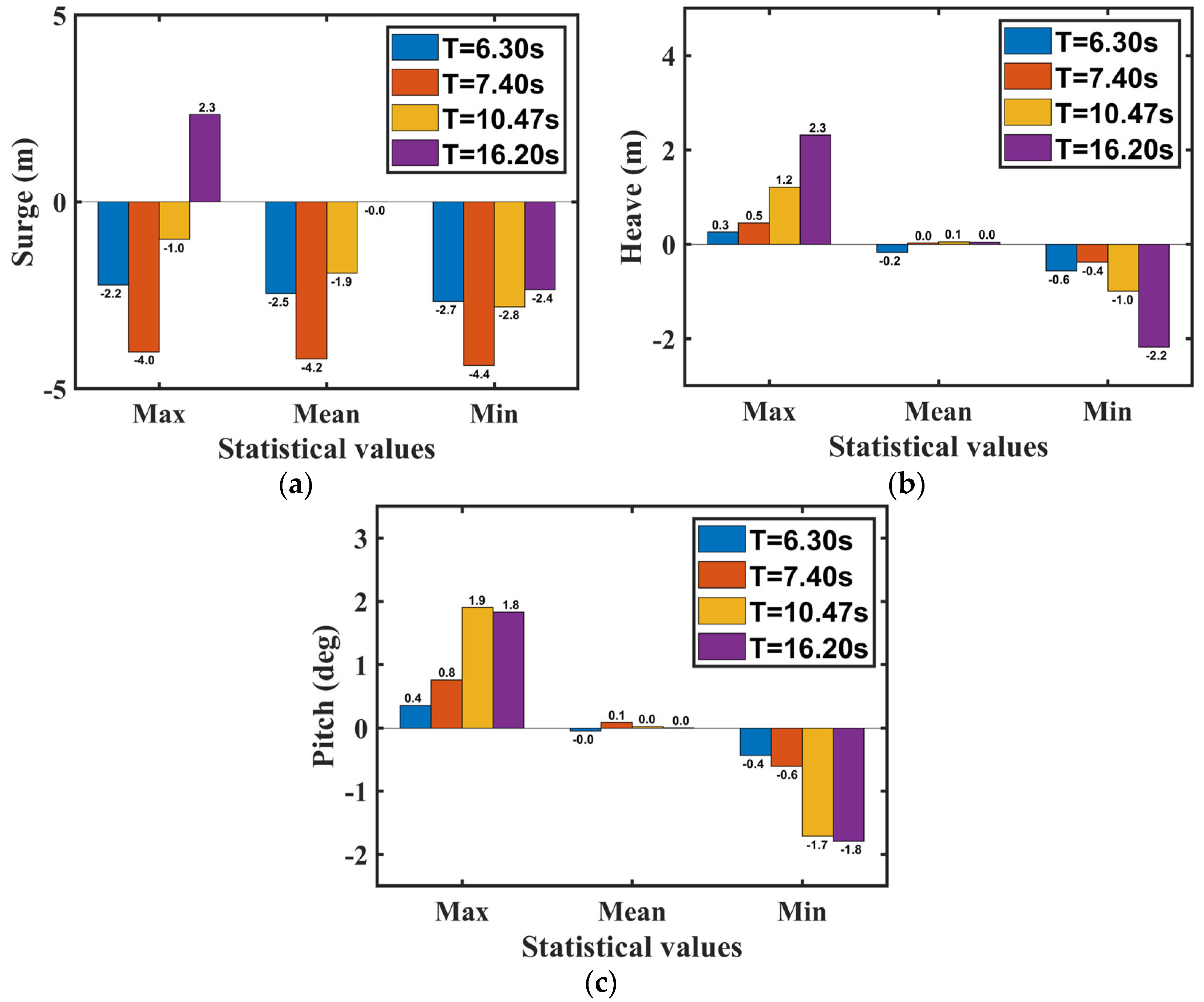
| LC3 | Head sea | 4.00 | 6.30, 7.40, 10.47, 16.20 | 0.08 | 0.89, 1.05, 1.48, 2.29 |
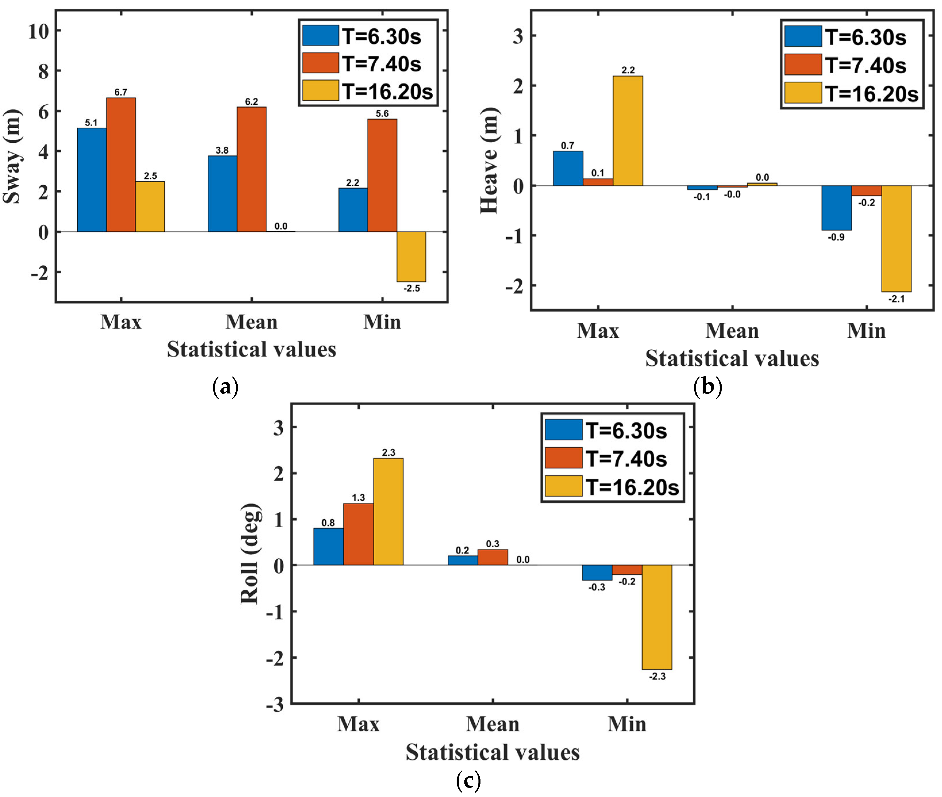
| LC4 | Beam sea | 4.00 | 6.30, 7.40, 16.20 | 0.08 | 0.89, 1.05, 2.29 |
| Number | Description | Full Scale | Model Tests | |||
|---|---|---|---|---|---|---|
| Hs (m) | Tp (s) | Hs (m) | Tp (s) | |||
| LC5 | Head sea | 2.50 | 7.00, 8.20, 11.60, 18.00 | 0.05 | 0.99, 1.16, 1.64, 2.55 | 1.90, 1.00, 1.00, 1.00 |
| LC6 | Beam sea | 2.50 | 7.00, 8.20, 18.00 | 0.05 | 0.99, 1.16, 2.55 | 1.90, 1.00, 1.00 |
| Number | Description | Full Scale | Model Tests | ||
|---|---|---|---|---|---|
| Hs (m) | T (s) | Hs (m) | T (s) | ||
| LC7 | 8 m, 12 m, 16 m | 2.50 | 5.00–20.00 | 0.05 | 0.71–2.83 |
| State | Freedom | Model Test | Tsimulation | Deviation | |||
|---|---|---|---|---|---|---|---|
| T1 | T2 | T3 | Taverage | ||||
| Unmoored state | Heave | 5.59 | 5.60 | 5.68 | 5.62 | 5.64 | −0.35% |
| Roll | 10.40 | 10.38 | 10.41 | 10.40 | 10.21 | 1.86% | |
| Pitch | 6.14 | 6.07 | 5.82 | 6.01 | 6.05 | −0.66% | |
| Head sea moored state | Surge | 77.54 | 78.01 | 78.76 | 78.10 | 76.20 | 2.49% |
| Heave | 5.66 | 5.66 | 5.66 | 5.66 | 5.65 | 0.19% | |
| Pitch | 6.06 | 6.08 | 6.07 | 6.07 | 6.08 | −0.12% | |
| Beam sea moored state | Sway | 61.46 | 60.66 | 60.87 | 61.00 | 58.51 | 4.24% |
| Heave | 5.81 | 5.81 | 5.81 | 5.81 | 5.65 | 2.80% | |
| Roll | 10.39 | 10.40 | 10.39 | 10.39 | 10.48 | −0.83% | |
| Load Case | Max | Mean | Min | |
|---|---|---|---|---|
| Surge (m) | Hs = 2.50 m, Tp = 7.00 s | 2.79 | −0.57 | −4.43 |
| H = 4.00 m, T = 6.30 s | −2.23 | −2.45 | −2.66 | |
| Hs = 2.50 m, Tp = 8.20 s | 3.05 | −0.56 | −4.42 | |
| H = 4.00 m, T = 7.40 s | −4.01 | −4.21 | −4.38 | |
| Hs = 2.50 m, Tp = 11.60 s | 2.81 | −0.35 | −3.70 | |
| H = 4.00 m, T = 10.47 s | −1.01 | −1.91 | −2.80 | |
| Hs = 2.50 m, Tp = 18.00 s | 2.16 | −0.09 | −2.62 | |
| H = 4.00 m, T = 16.20 s | 2.34 | 0.00 | −2.35 | |
| Heave (m) | Hs = 2.50 m, Tp = 7.00 s | 0.38 | −0.01 | −0.39 |
| H = 4.00 m, T = 6.30 s | 0.25 | −0.17 | −0.57 | |
| Hs = 2.50 m, Tp = 8.20 s | 0.60 | 0.00 | −0.52 | |
| H = 4.00 m, T = 7.40 s | 0.45 | 0.03 | −0.38 | |
| Hs = 2.50 m, Tp = 11.60 s | 1.48 | 0.01 | −1.24 | |
| H = 4.00 m, T = 10.47 s | 1.21 | 0.06 | −0.99 | |
| Hs = 2.50 m, Tp = 18.00 s | 2.13 | 0.01 | −2.01 | |
| H = 4.00 m, T = 16.20 s | 2.32 | 0.05 | −2.18 | |
| Pitch (deg) | Hs = 2.50 m, Tp = 7.00 s | 0.63 | 0.01 | −0.62 |
| H = 4.00 m, T = 6.30 s | 0.36 | −0.05 | −0.44 | |
| Hs = 2.50 m, Tp = 8.20 s | 0.90 | 0.00 | −0.87 | |
| H = 4.00 m, T = 7.40 s | 0.76 | 0.09 | −0.61 | |
| Hs = 2.50 m, Tp = 11.60 s | 1.82 | 0.00 | −1.71 | |
| H = 4.00 m, T = 10.47 s | 1.90 | 0.02 | −1.72 | |
| Hs = 2.50 m, Tp = 18.00 s | 1.86 | 0.00 | −1.85 | |
| H = 4.00 m, T = 16.20 s | 1.83 | 0.00 | −1.79 |
| Load Case | Max | Mean | Min | |
|---|---|---|---|---|
| Sway (m) | Hs = 2.50 m, Tp = 7.00 s | 7.85 | 1.13 | −4.89 |
| H = 4.00 m, T = 6.30 s | 5.14 | 3.77 | 2.16 | |
| Hs = 2.50 m, Tp = 8.20 s | 7.05 | 1.01 | −4.88 | |
| H = 4.00 m, T = 7.40 s | 6.65 | 6.19 | 5.60 | |
| Hs = 2.50 m, Tp = 18.00 s | 3.18 | 0.13 | −2.83 | |
| H = 4.00 m, T = 16.20 s | 2.50 | 0.01 | −2.48 | |
| Heave (m) | Hs = 2.50 m, Tp = 7.00 s | 0.61 | −0.04 | −0.67 |
| H = 4.00 m, T = 6.30 s | 0.69 | −0.09 | −0.89 | |
| Hs = 2.50 m, Tp = 8.20 s | 0.81 | 0.00 | −0.71 | |
| H = 4.00 m, T = 7.40 s | 0.14 | −0.04 | −0.21 | |
| Hs = 2.50 m, Tp = 18.00 s | 2.17 | 0.01 | −2.15 | |
| H = 4.00 m, T = 16.20 s | 2.19 | 0.05 | −2.13 | |
| Roll (deg) | Hs = 2.50 m, Tp = 7.00 s | 1.75 | 0.09 | −1.40 |
| H = 4.00 m, T = 6.30 s | 0.80 | 0.20 | −0.33 | |
| Hs = 2.50 m, Tp = 8.20 s | 3.00 | 0.06 | −2.86 | |
| H = 4.00 m, T = 7.40 s | 1.34 | 0.34 | −0.77 | |
| Hs = 2.50 m, Tp = 18.00 s | 3.75 | 0.00 | −3.62 | |
| H = 4.00 m, T = 16.20 s | 2.32 | 0.00 | −2.26 |
| Input | Output |
|---|---|
| X1, X2, X3……, X100 | X101 |
| X2, X3, X4……, X101 | X102 |
| …… | …… |
| X7780, X7781, X7782……, X7879 | X7880 |
| Input | Output | True Value |
|---|---|---|
| X7881, X7882, X7883……, X7980 | Y1 | X7981 |
| X7882, X7883, X7884……, X7980, Y1 | Y2 | X7982 |
| …… | …… | …… |
| Y7900, Y7901, Y7902…X7980, Y1, …, Y19 | Y20 | X8000 |
| Input | Output |
|---|---|
| X1, X2, X3……, X100 | X101-X120 |
| X2, X3, X4……, X101 | X102-X121 |
| …… | …… |
| X7761, X7762, X7763……, X7860 | X7861-X7880 |
| Input | Output | True Value |
|---|---|---|
| X7881, X7882, X7883……, X7980 | Y1-Y20 | X7981-Y8000 |
| 1 | 2 | 3 | 4 | 5 | 6 | Mean | |
|---|---|---|---|---|---|---|---|
| R2 | 0.9023 | 0.9985 | 0.9135 | 0.9171 | 0.9442 | 0.9275 | 0.9339 |
| MAE | 0.1019 | 0.0208 | 0.1330 | 0.1958 | 0.1356 | 0.1087 | 0.1160 |
| RMSE | 0.1173 | 0.0238 | 0.1601 | 0.2263 | 0.1609 | 0.1449 | 0.1389 |
| 1 | 2 | 3 | 4 | 5 | 6 | Mean | |
|---|---|---|---|---|---|---|---|
| R2 | 0.9693 | 0.9912 | 0.9373 | 0.9804 | 0.9490 | 0.9168 | 0.9573 |
| MAE | 0.0562 | 0.0493 | 0.1066 | 0.0926 | 0.1348 | 0.1166 | 0.0927 |
| RMSE | 0.0657 | 0.0568 | 0.1363 | 0.1100 | 0.1539 | 0.1553 | 0.1130 |
| Stepwise Iterative Model | Direct Multi-Step Model | |||
|---|---|---|---|---|
| Before Optimization | After Optimization | Before Optimization | After Optimization | |
| R2 | 0.8148 | 0.9339 | 0.9435 | 0.9573 |
| MAE | 0.1870 | 0.1160 | 0.1045 | 0.0927 |
| RMSE | 0.2290 | 0.1389 | 0.1276 | 0.1130 |
Disclaimer/Publisher’s Note: The statements, opinions and data contained in all publications are solely those of the individual author(s) and contributor(s) and not of MDPI and/or the editor(s). MDPI and/or the editor(s) disclaim responsibility for any injury to people or property resulting from any ideas, methods, instructions or products referred to in the content. |
© 2025 by the authors. Licensee MDPI, Basel, Switzerland. This article is an open access article distributed under the terms and conditions of the Creative Commons Attribution (CC BY) license (https://creativecommons.org/licenses/by/4.0/).
Share and Cite
Zhao, M.; Zheng, X.Y.; Zhang, S.; Qian, K.; Jiang, Y.; Liu, Y.; Duan, M.; Zhao, T.; Zhai, K. Hydrodynamic Performance and Motion Prediction Before Twin-Barge Float-Over Installation of Offshore Wind Turbines. J. Mar. Sci. Eng. 2025, 13, 995. https://doi.org/10.3390/jmse13050995
Zhao M, Zheng XY, Zhang S, Qian K, Jiang Y, Liu Y, Duan M, Zhao T, Zhai K. Hydrodynamic Performance and Motion Prediction Before Twin-Barge Float-Over Installation of Offshore Wind Turbines. Journal of Marine Science and Engineering. 2025; 13(5):995. https://doi.org/10.3390/jmse13050995
Chicago/Turabian StyleZhao, Mengyang, Xiang Yuan Zheng, Sheng Zhang, Kehao Qian, Yucong Jiang, Yue Liu, Menglan Duan, Tianfeng Zhao, and Ke Zhai. 2025. "Hydrodynamic Performance and Motion Prediction Before Twin-Barge Float-Over Installation of Offshore Wind Turbines" Journal of Marine Science and Engineering 13, no. 5: 995. https://doi.org/10.3390/jmse13050995
APA StyleZhao, M., Zheng, X. Y., Zhang, S., Qian, K., Jiang, Y., Liu, Y., Duan, M., Zhao, T., & Zhai, K. (2025). Hydrodynamic Performance and Motion Prediction Before Twin-Barge Float-Over Installation of Offshore Wind Turbines. Journal of Marine Science and Engineering, 13(5), 995. https://doi.org/10.3390/jmse13050995