An Integrated Design of Course-Keeping Control and Extended State Observers for Nonlinear USVs with Disturbances


Abstract
1. Introduction
- (1)
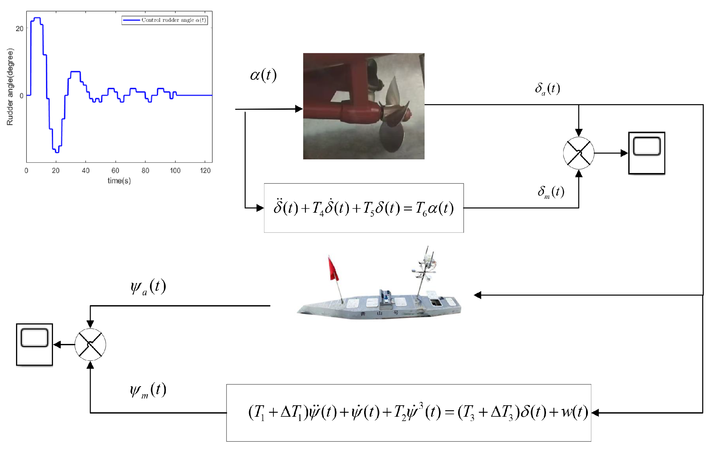
- To make the CCS more realistic, an integrated model is constructed that encompasses the characteristics of both the unmanned surface vehicle (USV) system and the rudder system. In the modeling process, the Norrbin model with parameter uncertainties is used to describe the USV system, while a second-order underdamped model is employed to represent the rudder system.
- (2)
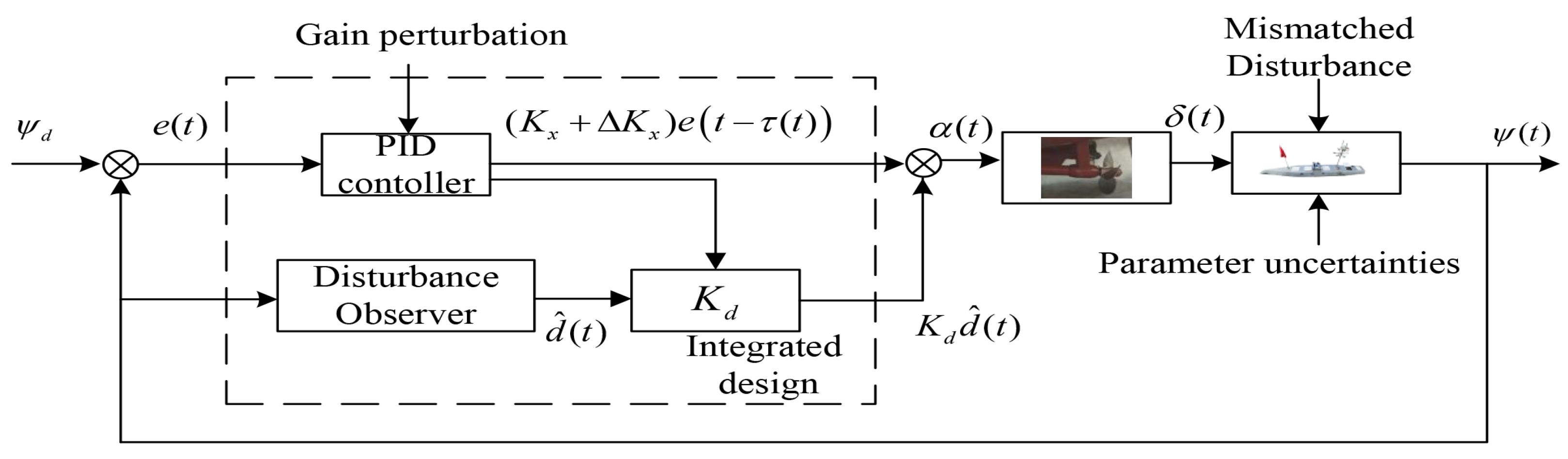
- A unified CCS strategy is proposed to address the perturbations in the controller, system parameter uncertainties, and the coupling between the controller and the extended state observer (ESO). This strategy aims to enhance the robustness and performance of the system by effectively managing the challenges posed by these factors.
2. Problem Formulation and Preliminaries
2.1. Structure of CCS
2.2. Characteristics of USV
2.3. Dynamics and Modeling of the Rudder Actuator
2.4. Integrated Model of CCS
- (1)
- ,
- (2)
- and ,
- (3)
- and .
3. Main Results
3.1. Extended State Observer
3.2. Integrated Design of Controller, Observer and Compensator
4. Simulation Example
4.1. Model Analysis
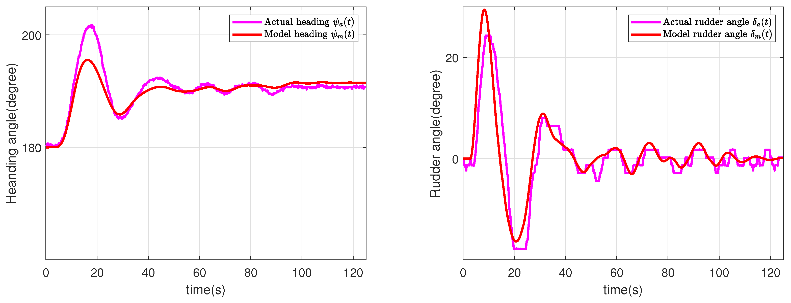
4.2. Example
5. Conclusions
Author Contributions
Funding
Data Availability Statement
Acknowledgments
Conflicts of Interest
References
- Lenzen, M.; Tzeng, M.; Floerl, O.; Zaiko, A. Application of multi-region input-output analysis to examine biosecurity risks associated with the global shipping network. Sci. Total Environ. 2023, 854, 158758. [Google Scholar] [CrossRef] [PubMed]
- Rousseau, Y.; Watson, R.A.; Blanchard, J.L.; Fulton, E.A. Evolution of global marine fishing fleets and the response of fished resources. Proc. Natl. Acad. Sci. USA 2019, 116, 12238–12243. [Google Scholar] [CrossRef]
- Cao, G.; Jia, Z.; Wu, D.; Li, Z.; Zhang, W. Trajectory tracking control for marine vessels with error constraints: A barrier function sliding mode approach. Ocean. Eng. 2024, 297, 116879. [Google Scholar] [CrossRef]
- Casanova, E.; Knowles, T.D.; Bayliss, A.; Walton-Doyle, C.; Barclay, A.; Evershed, R.P. Compound-specific radiocarbon dating of lipid residues in pottery vessels: A new approach for detecting the exploitation of marine resources. J. Archaeol. Sci. 2022, 137, 105528. [Google Scholar] [CrossRef]
- Li, S.; Cheng, X.; Shi, F.; Zhang, H.; Dai, H.; Zhang, H.; Chen, S. A novel robustness-enhancing adversarial defense approach to AI-powered sea state estimation for autonomous marine vessels. IEEE Trans. Syst. Man Cybern. Syst. 2024, 55, 28–42. [Google Scholar] [CrossRef]
- Zhao, L.; Bai, Y. Data harvesting in uncharted waters: Interactive learning empowered path planning for USV-assisted maritime data collection under fully unknown environments. Ocean. Eng. 2023, 287, 115781. [Google Scholar] [CrossRef]
- Zhang, J.; Han, G.; Sha, J.; Qian, Y.; Liu, J. AUV-assisted subsea exploration method in 6G enabled deep ocean based on a cooperative pac-men mechanism. IEEE Trans. Intell. Transp. Syst. 2021, 23, 1649–1660. [Google Scholar] [CrossRef]
- Nomoto, K.; Taguchi, K.; Honda, K.; Hirano, S. On the steering qualities of ships. J. Zosen Kiokai 1956, 1956, 75–82. [Google Scholar] [CrossRef]
- Inoue, S.; Hirano, M.; Kijima, K.; Takashina, J. A practical calculation method of ship maneuvering motion. Int. Shipbuild. Prog. 1981, 28, 207–222. [Google Scholar] [CrossRef]
- Kijima, K.; Katsuno, T.; Nakiri, Y.; Furukawa, Y. On the manoeuvring performance of a ship with theparameter of loading condition. J. Soc. Nav. Archit. Jpn. 1990, 1990, 141–148. [Google Scholar] [CrossRef]
- Norrbin, N.H. Theory and Observations on the Use of a Mathematical Model for Ship Manoeuvring in Deep and Confined Waters; Technical Report; National Technical Information Service: Springfield, VA, USA, 1971.
- Dong, Z.; Wan, L.; Li, Y.; Liu, T.; Zhang, G. Trajectory tracking control of underactuated USV based on modified backstepping approach. Int. J. Nav. Archit. Ocean. Eng. 2015, 7, 817–832. [Google Scholar] [CrossRef]
- Lei, T.; Wen, Y.; Yu, Y.; Tian, K.; Zhu, M. Predictive trajectory tracking control for the USV in networked environments with communication constraints. Ocean. Eng. 2024, 298, 117185. [Google Scholar] [CrossRef]
- Xiong, J.; Li, J.n.; Du, P. A novel non-fragile H∞ fault-tolerant course-keeping control for uncertain unmanned surface vehicles with rudder failures. Ocean. Eng. 2023, 280, 114781. [Google Scholar] [CrossRef]
- Qiu, B.; Wang, G.; Fan, Y. Trajectory linearization-based robust course keeping control of unmanned surface vehicle with disturbances and input saturation. ISA Trans. 2021, 112, 168–175. [Google Scholar] [CrossRef]
- He, Z.; Fan, Y.; Wang, G.; Qiao, S. Finite time course keeping control for unmanned surface vehicles with command filter and rudder saturation. Ocean. Eng. 2023, 280, 114403. [Google Scholar] [CrossRef]
- Wu, R.; Du, J.; Xu, G.; Li, D. Active disturbance rejection control for ship course tracking with parameters tuning. Int. J. Syst. Sci. 2021, 52, 756–769. [Google Scholar] [CrossRef]
- Do, M.H.; Koenig, D.; Theilliol, D. Robust H∞ proportional-integral observer-based controller for uncertain LPV system. J. Frankl. Inst. 2020, 357, 2099–2130. [Google Scholar] [CrossRef]
- Rodrigues, M.; Hamdi, H.; Braiek, N.B.; Theilliol, D. Observer-based fault tolerant control design for a class of LPV descriptor systems. J. Frankl. Inst. 2014, 351, 3104–3125. [Google Scholar] [CrossRef]
- Menhour, L.; Koenig, D.; d’Andréa Novel, B. Robust switched H∞ PI observer-based controller: Vehicle dynamics application. IFAC-PapersOnLine 2017, 50, 10377–10382. [Google Scholar] [CrossRef]
- Fossen, T. Marine Control Systems–Guidance, Navigation, and Control of Ships, Rigs and Underwater Vehicles; Marine Cybernetics: Trondheim, Norway, 2002; ISBN 82 92356 00 2. Available online: https://www.marinecybernetics.com (accessed on 1 March 2025).
- Mu, D.; Wang, G.; Fan, Y.; Sun, X.; Qiu, B. Modeling and identification for vector propulsion of an unmanned surface vehicle: Three degrees of freedom model and response model. Sensors 2018, 18, 1889. [Google Scholar] [CrossRef]
- Li, J.N.; Pan, Y.J.; Su, H.Y.; Wen, C.L. Stochastic reliable control of a class of networked control systems with actuator faults and input saturation. Int. J. Control. Autom. Syst. 2014, 12, 564–571. [Google Scholar] [CrossRef]
- Gu, K.; Chen, J.; Kharitonov, V.L. Stability and Stabilization of Time-Delay Systems; Birkhäuser: Boston, MA, USA, 2003. [Google Scholar]
- Xie, L. Output feedback H∞ control of systems with parameter uncertainty. Int. J. Control 1996, 63, 741–750. [Google Scholar] [CrossRef]
- Khorsand Zak, M.; Abbaszadeh Shahri, A. A Robust Hermitian and Skew-Hermitian Based Multiplicative Splitting Iterative Method for the Continuous Sylvester Equation. Mathematics 2025, 13, 318. [Google Scholar] [CrossRef]
- Abbaszadeh Shahri, A.; Shan, C.; Larsson, S.; Johansson, F. Normalizing Large Scale Sensor-Based MWD Data: An Automated Method toward A Unified Database. Sensors 2024, 24, 1209. [Google Scholar] [CrossRef] [PubMed]
- Yue, X. USV Course Control Strategy based on the Disturbance Observer Under Disturbances of Winds and Waves. In Proceedings of the 2023 Smart City Challenges & Outcomes for Urban Transformation (SCOUT), Singapore, 29–30 July 2023; pp. 76–80. [Google Scholar] [CrossRef]


Disclaimer/Publisher’s Note: The statements, opinions and data contained in all publications are solely those of the individual author(s) and contributor(s) and not of MDPI and/or the editor(s). MDPI and/or the editor(s) disclaim responsibility for any injury to people or property resulting from any ideas, methods, instructions or products referred to in the content. |
© 2025 by the authors. Licensee MDPI, Basel, Switzerland. This article is an open access article distributed under the terms and conditions of the Creative Commons Attribution (CC BY) license (https://creativecommons.org/licenses/by/4.0/).
Share and Cite
Wu, N.; Li, J.; Xiong, J. An Integrated Design of Course-Keeping Control and Extended State Observers for Nonlinear USVs with Disturbances. J. Mar. Sci. Eng. 2025, 13, 967. https://doi.org/10.3390/jmse13050967
Wu N, Li J, Xiong J. An Integrated Design of Course-Keeping Control and Extended State Observers for Nonlinear USVs with Disturbances. Journal of Marine Science and Engineering. 2025; 13(5):967. https://doi.org/10.3390/jmse13050967
Chicago/Turabian StyleWu, Nianzhe, Jianning Li, and Ju Xiong. 2025. "An Integrated Design of Course-Keeping Control and Extended State Observers for Nonlinear USVs with Disturbances" Journal of Marine Science and Engineering 13, no. 5: 967. https://doi.org/10.3390/jmse13050967
APA StyleWu, N., Li, J., & Xiong, J. (2025). An Integrated Design of Course-Keeping Control and Extended State Observers for Nonlinear USVs with Disturbances. Journal of Marine Science and Engineering, 13(5), 967. https://doi.org/10.3390/jmse13050967