The TSformer: A Non-Autoregressive Spatio-Temporal Transformers for 30-Day Ocean Eddy-Resolving Forecasting

Abstract

Ocean forecasting is critical for various applications and is essential for understanding air–sea interactions, which contribute to mitigating the impacts of extreme events. While data-driven forecasting models have demonstrated considerable potential and speed, they often primarily focus on spatial variations while neglecting temporal dynamics. This paper presents the TSformer, a novel non-autoregressive spatio-temporal transformer designed for medium-range ocean eddy-resolving forecasting, enabling forecasts of up to 30 days in advance. We introduce an innovative hierarchical U-Net encoder–decoder architecture based on 3D Swin Transformer blocks, which extends the scope of local attention computation from spatial to spatio-temporal contexts to reduce accumulation errors. The TSformer is trained on 28 years of homogeneous, high-dimensional 3D ocean reanalysis datasets, supplemented by three 2D remote sensing datasets for surface forcing. Based on the near-real-time operational forecast results from 2023, comparative performance assessments against in situ profiles and satellite observation data indicate that the TSformer exhibits forecast performance comparable to leading numerical ocean forecasting models while being orders of magnitude faster. Unlike autoregressive models, the TSformer maintains 3D consistency in physical motion, ensuring long-term coherence and stability. Furthermore, the TSformer model, which incorporates surface auxiliary observational data, effectively simulates the vertical cooling and mixing effects induced by Super Typhoon Saola.

1. Introduction

The oceans, constituting approximately 70.8% of the Earth’s surface, are the principal recipient of solar radiation. They facilitate the transfer of energy, heat, salt, carbon, and nutrients through seawater movement, resulting in significant marine phenomena, such as mesoscale eddies, which greatly influence marine life distribution and connectivity [1]. With a specific heat capacity four times that of air, the oceans absorb 93% of the heat generated by the greenhouse effect, transferring it to the deep oceans [2]. The Intergovernmental Panel on Climate Change sixth assessment report affirms the global average sea surface temperature (SST) increased by 0.88 °C between 1850 and 1900 and between 2011 and 2020, with 0.60 °C of this warming having occurred since 1980 [3]. Additionally, the complexity of the marine environment is manifested not only in the long-term effects of climate change but in the frequency of marine disasters, such as tropical cyclones (including typhoons and hurricanes), internal waves, and marine heatwaves [4]. Ocean forecasting is essential for addressing climate change, predicting extreme events, and providing a scientific foundation for tackling global challenges [5].

Over the past few decades, the accuracy of operational ocean forecasting has continually improved due to advancements in high-performance computing (HPC) and data assimilation methods [6]. Since the inaugural global simulations that achieved eddy resolution and visualized global ocean circulation in 1988 [7], contemporary global operational numerical forecasts now span a range of scales, from weather-scale resolutions of one kilometer to seasonal forecasts with resolutions in the tens of kilometers. These forecasts are facilitated by ocean numerical models, such as the Nucleus for European Modelling of the Ocean (NEMO) [8], which integrates diverse datasets including in situ profile data, altimeter data, surface temperature data, and sea ice observations. At present, the leading operational global ocean forecasting systems (GOFSs), such as the Mercator Ocean Physical System (PSY4) and the Real-Time Ocean Forecast System (RTOFS), use physics-driven models in fluid mechanics and thermodynamics with HPC to predict future ocean motion states and phenomena based on current ocean conditions. These systems cover global-to-coastal marine environments and physical and biogeochemical properties, with forecasts typically extending up to 10 days in advance [6].

The augmentation of HPC capabilities has facilitated an escalation in the horizontal resolution of global ocean models, transitioning from 1/10° to 1/32°. This enhancement has led to substantial improvements in the simulation of critical oceanographic phenomena, including surface eddy kinetic energy, the principal pathways of the Kuroshio and Gulf Stream currents, and global tidal dynamics [9]. Compared to their lower-resolution counterparts, high-resolution models within the Community Earth System Model are now capable of directly simulating small- to medium-scale atmospheric and oceanic extreme phenomena, such as tropical cyclones, ocean eddies, and frontal systems [10]. However, the computational and operational demands for ocean simulations at appropriate spatial and temporal scales are substantial, necessitating HPC to deliver forecasts and services within practical timeframes. The research indicates that elevating the resolution from 1/10° to 1/32° results in an approximate increase in computational load and memory overhead by a factor of 32 and 10, respectively [11], posing significant technical challenges for model development and operational efficiency.

On the other hand, deep learning technology, characterized by its rapid computational prowess, has furnished ocean forecasting with more robust tools and methodologies. Over the past decade, the exponential expansion of spatio-temporal earth observation and reanalysis datasets has catalyzed the emergence of data-driven models that harness deep learning [12]. These models are showing remarkable potential across a range of earth system forecasting tasks, such as the nowcasting of extreme precipitation [13,14], ocean forecasting [15,16], climate predictions [17,18], and ocean phenomenon recognition [19]. Prior research has amalgamated recurrent neural networks (RNNs) and convolutional neural networks (CNNs) to leverage temporally and spatially induced biases, effectively capturing spatio-temporal patterns [20,21]. The CNN methods, utilizing satellite observations and gridded arrays for real-time geostrophic oceanography Project Argo data, have been extensively employed in the reconstruction and prediction of long-lead monthly three-dimensional ocean temperatures [22], as well as in forecasting surface 2D ocean environmental factors, such as the SST and the Sea-Level Anomaly (SLA) [23]. These intelligent identification and forecasting methods exhibit significant advantages in terms of computational efficiency and predictive accuracy over conventional methodologies [24].

Recently, the transformers and their variants have exhibited exceptional performance across a spectrum of computer vision tasks [25,26]. Renowned for their exceptional parallel computing capabilities and ability to capture long-range dependencies, transformers have made it feasible to train extremely large parameter models. Notably, the advanced transformer-based forecasting models have become shockingly good at forecasting the weather while using fewer resources than numerical modeling systems [27]. For example, FourCastNet, which employs the adaptive Fourier neural operator architecture, can generate medium-range weather forecasts globally with an accuracy nearing state-of-the-art, while being five orders-of-magnitude faster than physics-based numerical weather prediction [28]. GraphCast, trained on reanalysis data, predicts hundreds of weather variables for the next 10 days at a 0.25° global resolution within 1 min, enhancing severe event prediction, including tropical cyclone tracking, atmospheric rivers, and extreme temperatures [29]. Pangu-Weather, incorporating a 3D Earth-specific transformer architecture and hierarchical temporal aggregation strategy, yields superior deterministic forecast results on reanalysis data compared to the European Centre for Medium-Range Weather Forecasts (ECMWF) Integrated Forecast System (IFS), the world’s leading numerical weather prediction system, while also achieving significantly faster computational performance [30].

In comparison to computer vision tasks, 3D ocean variables, such as 3D temperature and salinity (3D TS), present higher dimensionality and resolution, and encompass more intricate physical processes. The representation of these 3D variables necessitates a significantly larger number of input tokens. The global self-attention mechanism employed in the transformer architecture is impractical for data with high dimensionality and resolution due to its computational complexity, which scales quadratically with the size of the 3D data. To overcome the computational limitations of global self-attention, the Swin Transformer introduces a window-based self-attention mechanism [31]. This approach partitions the input tensor into non-overlapping local windows and computes self-attention independently within each window. By restricting attention to fixed-size windows, the computational complexity is linear with respect to the number of tokens, effectively addressing the scalability challenges of traditional transformers [32]. Additionally, the model preserves cross-window interactions through hierarchical shifts, balancing efficiency with global contextual understanding. The FuXi model employs a 48-layer architecture composed of stacked Swin Transformer V2 blocks [33] to generate 15-day global weather forecasts. The model operates at a 6-h temporal resolution and a 0.25° spatial resolution, achieving high-frequency updates while maintaining fine-grained atmospheric representation [34]. Furthermore, FuXi-S2S demonstrates an enhanced ability to capture forecast uncertainty and accurately predict the Madden–Julian oscillation (MJO), extending the skillful MJO prediction from 30 to 36 days [35]. Additionally, the XiHe model, a data-driven global ocean eddy-resolving forecasting model with a 1/12° resolution, employs a hierarchical Swin-transformer-based framework coupled with a land–ocean mask mechanism and ocean-specific blocks to effectively capture both local ocean information and global teleconnections [36]. These advancements in data-driven forecasting models have resulted in valuable tools for identifying precursor signals, providing researchers with insights, and potentially heralding a new paradigm in earth system science research.

However, training a large-scale Swin Transformer model for high-resolution ocean forecast reveals several issues, including training instability. Modeling the spatio-temporal dynamics of 3D ocean variables presents a significant challenge for deep learning architectures. Current data-driven forecasting models predominantly emphasize the 3D spatial aspects of ocean data through the deployment of 3D neural networks. These models often utilize autoregressive techniques for temporal forecasting to mitigate computational demands, thereby neglecting the system’s temporal evolution. Given the chaotic nature of ocean systems, the variability is acutely responsive to both initial spatial states and temporal fluctuations. The efficacy of integrating spatio-temporal attention mechanisms into RNN and transformer models for these complex systems remains an open question. Beyond minimal adaptation from the Swin Transformer, recent studies have incorporated additional induced biases into the design of space–time transformers, including trajectory [37], Multiscale Vision Transformers [38], and Multiview Transformer [39] approaches. However, no prior research has explicitly focused on the development of space–time transformers for the specific purpose of 3D TS forecasting.

In this study, we introduce the TSformer, a novel non-autoregressive spatio-temporal Transformer specifically crafted for medium-range ocean eddy-resolving forecasting of 3D TS, with a forecasting time scale of up to 30 days. The TSformer model is meticulously engineered to efficiently extract complex 3D features and infer relationships from consistent, homogeneous, high-dimensional ocean datasets. Notably, the TSformer model development leverages a 28-year daily ocean physical reanalysis dataset with a spatial resolution of 0.08°. Employing the pre-trained model parameters, we integrated near real-time satellite remote sensing data as surface forcing and utilized the 3D TS nowcast fields as initialization inputs to assess the forecast outcomes for the year 2023. The evaluation, based on in situ and satellite observations, indicates that the TSformer matches with the PSY4 numerical forecast results. Furthermore, as exemplified by Super Typhoon Saola (2309), the TSformer surpass those of other deep-learning models in accuracy, especially concerning the SST cooling response, due to the integration of auxiliary observational data.

2. Data

2.1. 3D Eddy-Resolving Ocean Physical Reanalysis Data

In this study, we employ global eddy-resolving physical ocean and sea ice reanalysis data (GLORYS12V1) for training and validation in deep learning. The GLORYS12V1 product is the Copernicus Marine Environment Monitoring Service (CMEMS) global ocean eddy-resolving (1/12° horizontal resolution, approximatively 8 km, 50 vertical levels, daily mean) reanalysis covering the altimetry (https://resources.marine.copernicus.eu/product-detail/GLOBAL_MULTIYEAR_PHY_001_030/, accessed on 10 May 2025),which provides a high-quality and consistent global ocean reanalysis product [40]. It utilizes the NEMO ocean numerical model, which is driven at surface by the European Centre for Medium Range Weather Forecasts ERA-Interim then ERA5 reanalysis for recent years. Observations are assimilated by means of a reduced-order Kalman filter. Along track altimeter data, satellite SST, sea ice concentration, and in situ temperature and salinity vertical profiles are jointly assimilated. Moreover, a 3D-VAR scheme provides a correction for the slowly-evolving large-scale biases in temperature and salinity.

2.2. 2D Remote Sensing Auxiliary Dataset for Surface Forcing

The wealth of 2D Ocean satellite remote sensing observations is crucial for advancements in marine science and oceanographic numerical forecasting. This study utilizes three long-term delay-time ocean satellite surface observations as auxiliary data to extract meaningful features from these observations. The multisatellite altimeter SLA dataset is distributed by Archiving, Validation and Interpretation of Satellite Oceanographic (AVISO), which provides a consistent and homogeneous catalog of products. The gridded wind speed (SPD) product are from the Cross Calibrated Multi-Platform (CCMP) V3.1 dataset, which provides Gap-free ocean surface wind data of high quality and high temporal and spatial resolution [41]. The CCMP is a combination of ocean surface (10 m) wind retrievals from multiple types of satellite microwave sensors and a background field from reanalysis. The SST data are from the Operational Sea Surface Temperature and Sea Ice Analysis (OSTIA) system [42], which provides daily gap-free maps of foundation SST and ice concentration at 0.05 deg. × 0.05 deg. horizontal grid resolution, using in situ and satellite data.

2.3. Evaluation Dataset

The Argo is an international program that aims to rapidly, accurately, and extensively collect temperature and salinity profile data from the upper layers of the global oceans to improve the accuracy of climate forecasts and effectively defend against the threats posed to humanity by increasingly severe global climate disasters, such as hurricanes, tornadoes, ice storms, floods, and droughts [43]. In this paper, we utilize the 941 Argo profiles from 2023 that have undergone delayed-mode quality control to assess and evaluate the forecasting capabilities of the TSformer (Figure 1). The process of Argo profiles includes routine quality control, such as duplication removal, landing inspection, climatological boundary examination, spike inspection, and stability testing, as well as salinity drift calibration [44].

In addition, to further examine the response of the SST to typhoons, we have evaluated the SST forecasts based on the Optimally Interpolated (OI) daily SST products using microwave and infrared data (MW_IR) at a 9 km resolution (MW_IR OI SST). The 9 km MW_IR OI SST product combines the through-cloud capabilities of the microwave data with the high spatial resolution and near-coastal capability of the infrared SST data, which can still obtain reliable SST observations even under extreme weather conditions, such as heavy rainfall during typhoons [45].

2.4. Data Pre-Processing and Model Domain

This study focuses on forecast 3D TS with a spatial resolution of 1/12° and a vertical resolution of 26 elevation levels, utilizing three 2D remote sensing datasets (SLA, SST, and SPD) as auxiliary data for surface forcing. Consistent with the prior research, the dataset is divided into training, validation, and testing sets. The training subset encompasses 10,227 samples from 1993 to 2020, the validation subset includes 730 samples from 2021 to 2022, and out-of-sample near real-time testing is performed with 365 samples from 2023. To enhance the convergence rate of the gradient descent algorithm, the training subset is normalized to the interval [−1, 1] using min–max scaling, with land points assigned a value of zero. The same normalization parameters derived from the training subset are applied to the validation and test subsets.

The spatio-temporal sequence of the 3D TS forecasting problem is designed to predict the most likely future output time steps (Tout) and the H × W × D grid of the 3D TS sequences, based on the current 3D TS sequence and the auxiliary observations at the preceding input time steps (Tin). This mathematical relationship is formalized in Equation (1).

$$\begin{array}{l}3D\hspace{1em}{\stackrel{\wedge }{TS}}_{T+1:T+Tout}=\underset{3D\hspace{1em}T{S}_{T-Tin:T}}{\arg \max p}(3D T{S}_{T-Tin:T}|AU{X}_{T-Tin:T})\\ AU{X}_{T-Tin:T}=\left\{SL{A}_{T-Tin:T},SST{A}_{T-Tin:T},SPD{A}_{T-Tin:T}\right\}\end{array}$$

(1)

We define the sequences of the 3D TS sequence as a series of matrices $3D\hspace{1em}T{S}_{T-Tin:T}=\left[3D\hspace{1em}T{S}_{T-Tin},3D\hspace{1em}T{S}_{T-Tin+1},...,3D\hspace{1em}T{S}_T\right]$, where the auxiliary observations are represented as a series of matrices $AU{X}_{T-Tin:T}$, each contains a set of SLA, SST, and SPD data. The input and output datasets for the 3D TS model are configured with dimensions of [Tin × H × W × D] and [Tout × H × W × D], respectively. Auxiliary data are formatted to the size of [Tin × H × W × Daux], where Tin and Tout denote the input and output time steps, respectively. Considering the large specific heat capacity of the ocean, which results in a relatively slow response of ocean temperature and salinity to external forcing, both Tin and Tout are set to 10 days to adequately capture the spatio-temporal characteristics of the oceanic system. The variables D and Daux correspond to the vertical levels and sea surface satellite variables, with D assigned to 26 and Daux to 3 in this study. H and W signify the dimensions of the regular latitude/longitude grid. All auxiliary data are uniformly processed to a 1/12° spatial resolution using bilinear interpolation.

Given the significant GPU (graphics processing unit) resources necessary for training high-resolution global ocean forecast models—such as Pangu-Weather, which operates at a 1/4° global spatial resolution and requires approximately 16 days on a cluster of 192 NVIDIA Tesla-V100 GPUs during training [30]—this study concentrates on forecasting within the spatial domain of the South China Sea (SCS), spanning 100–130° E and 0–30° N, with spatial dimensions (H and W) set to 360 each. The SCS, located south of mainland China, is the largest semi-enclosed marginal sea in the northwestern Pacific Ocean and is known for its frequent typhoons (refer to Figure 1). Due to its complex topography and the influence of strong seasonal monsoons, improving the forecast accuracy of the marine environment in the SCS presents a longstanding and significant challenge [46,47].

3. Methods

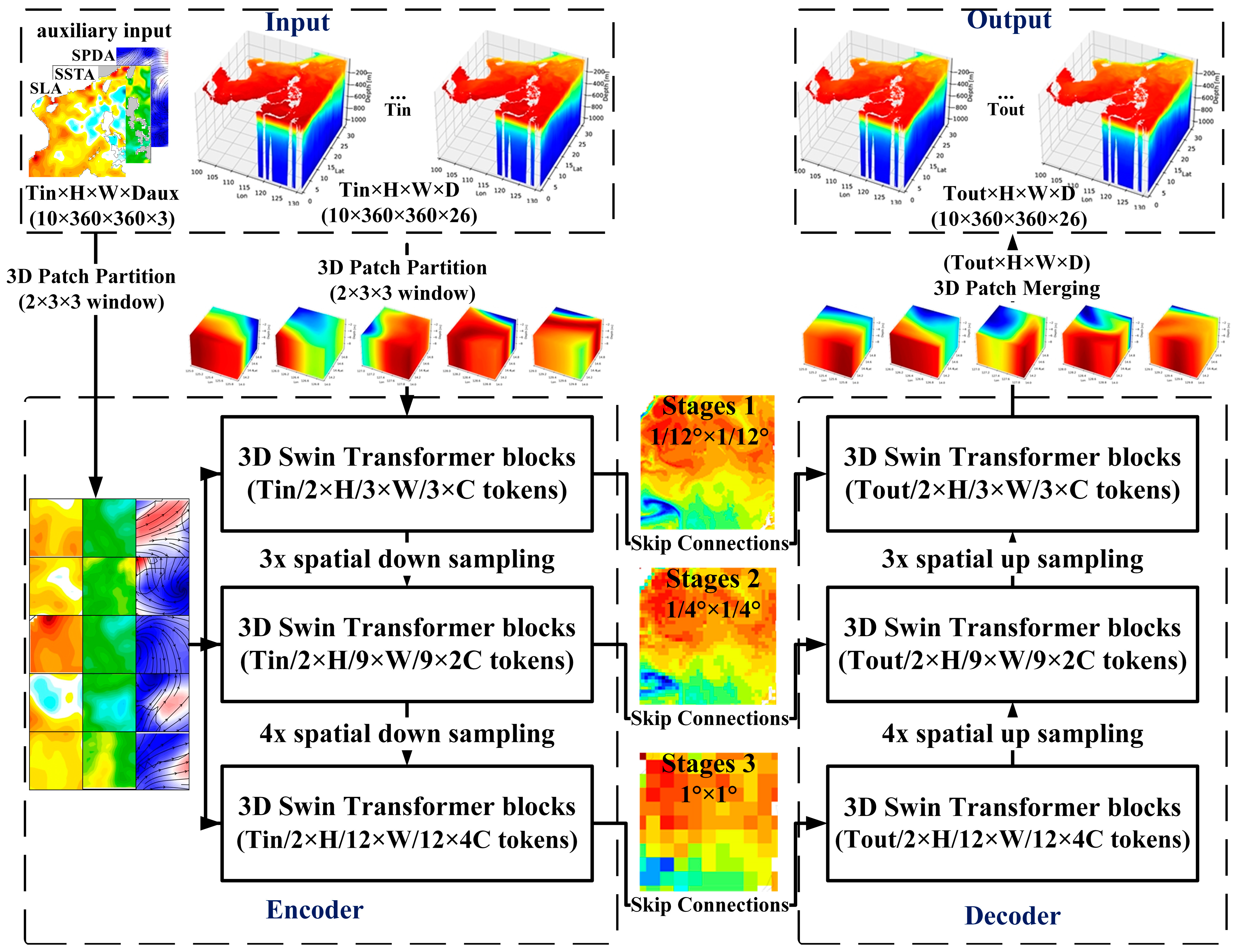
3.1. TSformer Model Architecture

The TSformer model employs a hierarchical U-Net encoder–decoder framework that leverages 3D Swin Transformer blocks to systematically encode the input sequence into a hierarchy of representations and facilitate forecasting through a coarse-to-fine approach. This architecture consists of four primary components, as depicted in Figure 2. Firstly, the extensive input dataset undergoes dimensionality reduction via joint spatio-temporal 3D Patch Partitioning process, which effectively reduces the complexity of the input data while preserving critical spatio-temporal features. Subsequently, a U-Net structure is employed for downsampling to extract features across multiple scales, capturing both local and global patterns in the data. The 3D tokens generated from the previous steps are then passed through a U-shaped encoder–decoder architecture, founded on 3D Swin Transformer blocks and incorporating skip connections to preserve spatial and temporal information. The encoder processes the input data hierarchically, generating multi-scale memory outputs, which are utilized by the decoder along with auxiliary inputs to perform comprehensive spatio-temporal feature learning. Finally, the 3D Patch Merging operation reintegrates the processed sub-regions to reconstruct the original output configuration, ensuring that the forecasted data retains the spatial and temporal coherence of the input data. Detailed information on each component within the TSformer model is provided in the subsequent sections.

The 3D Patch Partitioning process treats each 3D patch of size 2 × 3 × 3 as a token, partitioning the high-dimensional input data into manageable sub-regions to enhance processing efficiency. This partitioning results in the extraction of [Tin/2 × H/3 × W/3] 3D tokens, with each token encompassing a 522-dimensional feature (2 × 3 × 3 × D + 2 × 3 × 3 × Daux). Once the 3D tokens are derived from both the 3D TS data and the 2D auxiliary inputs, a linear embedding layer is applied to project the token features into an arbitrary dimension, denoted by C, which represents the base channel width, and is set to 256 in this context.

The encoder, which employs a hierarchical U-Net architecture, is engineered to capture contextual information and extract features from the input 3D tokens across three stages. Except for the initial stage, each stage begins by downsampling the input feature map to reduce resolution, thereby increasing the receptive field to encompass global information. During the second stage, the patch merging layer achieves a 3× spatial downsampling (1/4° × 1/4°); in the third stage, it performs a 4× spatial downsampling (1° × 1°). The encoder is composed of three 3D Swin Transformer blocks and two downsampling layers, which are designed to progressively reduce the spatial resolution of the original 3D ocean data (1/12° × 1/12°) while expanding the number of feature maps. This design aids the model in capturing higher-level features. The 3D Swin Transformer block is instrumental in computing correlations among various spatio-temporal elements, enabling the detection of long-term trends, periodicity, and 3D spatial features within the data. Through these three stages, high-level features for small-scale (1/12° × 1/12°), medium-scale (1/4° × 1/4°), and large-scale (1° × 1°) ocean data are sequentially extracted. This methodology facilitates the efficient extraction of multi-scale spatio-temporal features from the 3D ocean data, leading to a comprehensive understanding of the spatio-temporal characteristics within the dataset.

The decoder, adhering to the U-Net architectural paradigm, is responsible for the incremental upscaling of feature spatio-temporal dimensions. It plays a critical role in merging features from the downsampling path using skip connections. Consisting of three 3D Swin Transformer blocks and two upsampling layers, the decoder receives multi-scale feature outputs from the corresponding encoder block and the preceding decoder stage. Each upsampling layer skillfully integrates these inputs. The strategic integration of skip connections alongside 3D Swin Transformer blocks within the decoder architecture is essential for reconstructing the original spatial and temporal attributes of the 3D ocean dataset and its auxiliary inputs.

The 3D Patch Merging process, occurring in the final stage of the decoder, is crucial for transforming feature maps into the ultimate 3D forecasting field. It serves as the inverse of the 3D Patch Partition process, meticulously reassembling the processed sub-regions to reconstruct the 3D output with precision.

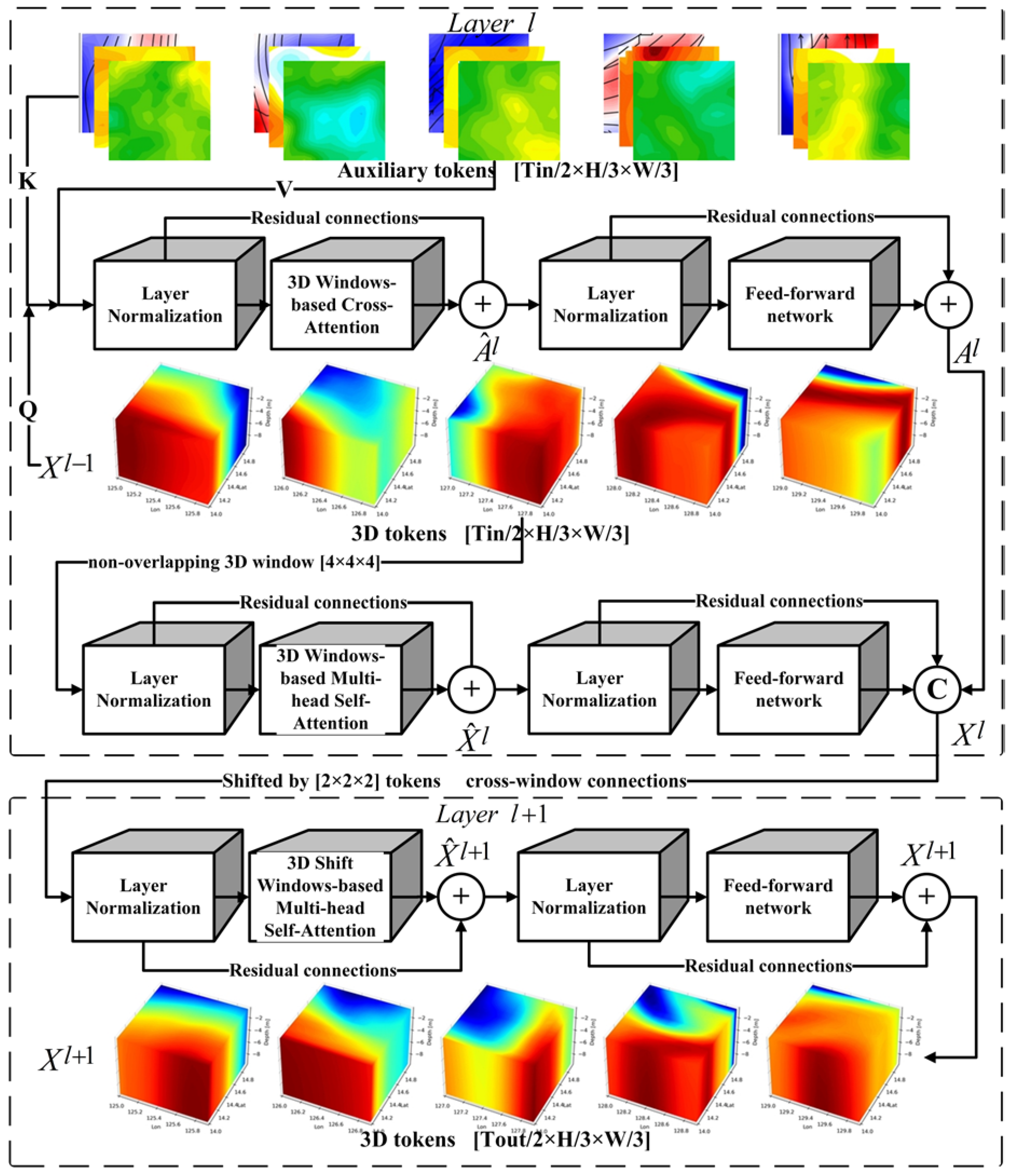
3.2. 3D Swin Transformer Block

We propose the 3D Swin Transformer block (see Figure 3), which is designed to address various data correlations, including temporal and spatial correlations, by employing multiple structure-aware space–time attention layers. This methodology extends the scope of local attention from purely spatial to encompass spatio-temporal computations. Consequently, the TSformer is capable of capturing the intricate temporal dynamics among different variables and extracting fine-grained spatial features across various vertical layers. This dual capability significantly bolsters the model’s forecasting accuracy.

The computation formula of the 3D Swin Transformer block is shown in Equation (2).

$$\begin{array}{l}{\widehat{A}}^l=3D\text{-}W\text{-}CA(LN(A^{l-1}))+A^{l-1},\\ A^l=FFN(LN({\widehat{A}}^l))+{\widehat{A}}^l,\\ {\widehat{X}}^l=3D\text{-}W\text{-}MSA(LN(X^{l-1}))+X^{l-1},\\ X^l=FFN(LN({\widehat{X}}^l))+{\widehat{X}}^l,\\ {\widehat{X}}^{l+1}=3D\text{-}SW\text{-}MSA(LN(concat(X^l,A^l)))+concat(X^l,A^l),\\ X^{l+1}=FFN(LN({\widehat{X}}^{l+1}))+{\widehat{X}}^{l+1},\end{array}$$

(2)

where ${\widehat{A}}^l$ and ${\widehat{X}}^l$ denote the output features of the 3D window-based cross-attention (3D-W-CA) module and the 3D window-based multi-head self-attention (3D-W-MSA) module for block $l$, respectively; layer normalization (LN) refers to the process of normalizing inputs across the features of a layer to stabilize and accelerate training; $A^l$ and $X^l$ denote the output features of the feed-forward network (FFN) module for block $l$, respectively; ${\widehat{X}}^{l+1}$ and $X^{l+1}$ denote the output features of the 3D shifted window-based multi-head self-attention (3D-SW-MSA) module and FFN module for block $l+1$, respectively.

In the 3D Swin Transformer block, the 3D TS data and auxiliary data are initially divided into spatio-temporal cuboid patches. These patches are then processed by two distinct modules: the 3D-W-CA module and the 3D-W-MSA module [48]. The 3D-W-CA module calculates the correlation and weighted sum between different sequences of the 3D TS and auxiliary input tokens, representing an advanced form of multi-head attention. This allows the model to capture cross-correlations between the primary data and auxiliary information effectively. Conversely, the 3D-W-MSA module focuses on analyzing the relationships between elements within the same input 3D TS sequence. By performing such an analysis, it reveals the intrinsic features of the 3D TS data, which is crucial for enhancing the model’s long-term forecasting capabilities. Subsequently, the attended weights generated by the FFN module are concatenated to reconstruct the output feature maps. This entire process enables the 3D Swin Transformer block to capture the complex spatio-temporal patterns within the 3D TS and auxiliary data through the synergistic operation of the 3D-W-CA and 3D-W-MSA modules. Finally, the 3D-SW-MSA module incorporates a shift window mechanism to introduce cross-window connections between adjacent non-overlapping 3D cuboid windows from the previous layer. This design enhances the model’s ability to capture long-range dependencies and contextual information across different spatial and temporal regions, thereby improving the overall forecasting accuracy and robustness of the TSformer model.

3.3. Non-Autoregressive Methods

Unlike traditional autoregressive models, which iteratively generate multi-step predictions through sequential single-step outputs (a process prone to amplified errors over extended lead times) [29], the TSformer directly produces multi-step forecasts in a single operation. For example, it leverages historical 3D TS data and auxiliary observations from the preceding 10-day period to predict the 3D TS fields for the subsequent 10 days. By treating the prediction window as an integrated unit, this design dramatically reduces iterative steps—generating a 30-day forecast requires only three iterations, whereas traditional autoregressive models demand 30 sequential single-step predictions, thereby significantly mitigating error propagation risks. The TSformer captures spatio-temporal patterns of ocean dynamics by processing continuous 10-day historical sequences, mirroring the 4D variational data assimilation (4D-Var) method’s emphasis on optimizing initial conditions through assimilation windows [49,50]. Both approaches prioritize harmonizing model predictions with observational data within defined temporal spans to enhance initial field accuracy and forecast coherence [51,52]. Although the TSformer, as a purely data-driven model, does not explicitly integrate physical equations, its window-based training strategy implicitly enforces temporal physical consistency, akin to the 4D-Var’s constraints on aligning model states with observations over time windows. However, challenges persist in managing error propagation across windows during iterative predictions and exploring the potential integration of explicit physical constraints to improve prediction realism.

3.4. Train and Hyperparameters

The TSformer model, developed utilizing the PyTorch Lightning framework (version 2.0.1), comprises approximately 222 million parameters, with hyperparameters detailed in

Table 1. Hyperparameters for training the TSformer model.

Hyperparameters	Value
Input Size	10 × 360 × 360 × 26
	10 × 360 × 360 × 3
Output Size	10 × 360 × 360 × 26
Loss Function	RMSE
Optimizer	AdamW
Learning Rate	0.001
β1	0.9
β2	0.999
Batch Size	16
Weight Decay	0.00001
Learning Rate Decay	Cosine
Max Training Epochs	200
Warm Up Percentage	10%
Early Stop	True
Early Stop Patience	10
Parameters	222 million

. The pretraining phase of the TSformer is anticipated to last around 10 days, utilizing a cluster of 8 Nvidia A800 GPUs. We employ the AdamW optimizer [53], setting β1 to 0.9 and β2 to 0.999, and incorporate a negative slope of 0.1 for the LeakyReLU activation function. The training process spans 200 epochs across all datasets, with early stopping initiated based on the validation score, permitting a patience of 10 epochs. A 20% linear warm-up phase precedes the cosine learning rate scheduler, which gradually decreases the learning rate to zero after the warm-up period. To mitigate memory consumption, a Fully Sharded Data Parallel [54] is implemented during training. Considering the high-resolution and high-dimensional nature of the dataset, the TSformer may require a larger parameter set and extended training durations. Therefore, practical deployment might require customized adjustments and optimizations to align with specific task demands and resource constraints.

4. Operational Forecast Results

To evaluate the operational forecasting performance of the TSformer model, we integrated near real-time satellite remote sensing data as surface forcing and utilized the 3D TS nowcast fields from the Operational Mercator global ocean analysis and forecast system, which is part of the real-time global forecasting CMEMS system [55]. This system closely mirrors the GLORYS12 reanalysis dataset [40]. These fields were used as initialization inputs for our model throughout 2023.

The TSformer operates daily, providing forecasts from 1 January 2023 to 31 December 2023, offering forecasts leading to 30 days. The physical 30-day forecast products from the TSformer, hereafter referred to as the 3D TS forecast results, include daily mean 3D TS fields on standard 1/12° grid (0.0833° latitude × 0.0833° longitude) in the SCS, with 26 geopotential levels ranging from 0 to 1000 m, consistent with the resolution of the GLORYS12 reanalysis data.

The accuracy of the 3D TS forecast results was evaluated using the 2023 evaluation dataset. The assessment involved out-of-sample 3D TS reanalysis datasets, quality-controlled Argo observations at delayed times (reprocessed when available), and independent WM_IR SST data. It is essential to underline that the uncertainty in analyzing the SST and observations is higher in near real-time forecasts compared to hindcast runs.

4.1. Metrics

We objectively assessed the accuracy and skill of the 3D TS forecasts from two distinct perspectives. Accuracy is determined by the discrepancy between the forecast and the observations or analyses, while skill is evaluated by comparing the forecast performance to a reference method, such as persistence or an alternative forecast system. The persistence model posits that the initial forecast state remains unchanged throughout the entire lead time [56], and it represents a cost-effective forecasting approach [57]. The alternative forecast systems used in this paper includes the PSY4 numerical forecast system, the TSformer model without auxiliary observational data (TSformer-w/o-aux), and the TSformer model integrated with autoregressive methods (TSformer-AR).

The evaluation was conducted using three principal performance indicators: bias, root mean square error (RMSE), mean relative error (MRE), and anomaly correlation coefficient (ACC). Bias indicates the presence of systematic errors, a perfect score of Bias = 0 does not preclude the possibility of large errors with opposite signs that may cancel each other out, thus the concurrent use of RMSE is essential for a comprehensive assessment. The RMSE, a widely accepted measure of accuracy, shows that higher values correspond to poorer forecasting proficiency. On the other hand, the ACC is regarded as a skill metric relative to climatology, with higher values indicating superior forecast skill. An ACC value of 0.5 suggests that the forecast errors are comparable to those of a forecast based on climatological averages alone.

$$Bias=\overline{f-o}$$

(3)

$$RMSE=\sqrt{\overline{{(f-o)}^2}}$$

(4)

$$MRE=\overline{\left|(f-o)/o\right|}$$

(5)

$$ACC=\overline{(f-c)(o-c)}{\sqrt{\overline{{(f-c)}^2}\overline{{(o-c)}^2}}}^{-1}$$

(6)

In this context, $f$ denotes the forecast value, while $o$ represents the observed or analyzed value. The climate value, indicated by $c$, is defined as the long-term average conditions of the ocean over a specified reference period. For the purposes of this paper, the reference period extends from 1993 to 2010. The over-bar symbol (-) signifies an average computed over an extensive sample, encompassing both temporal and spatial dimensions.

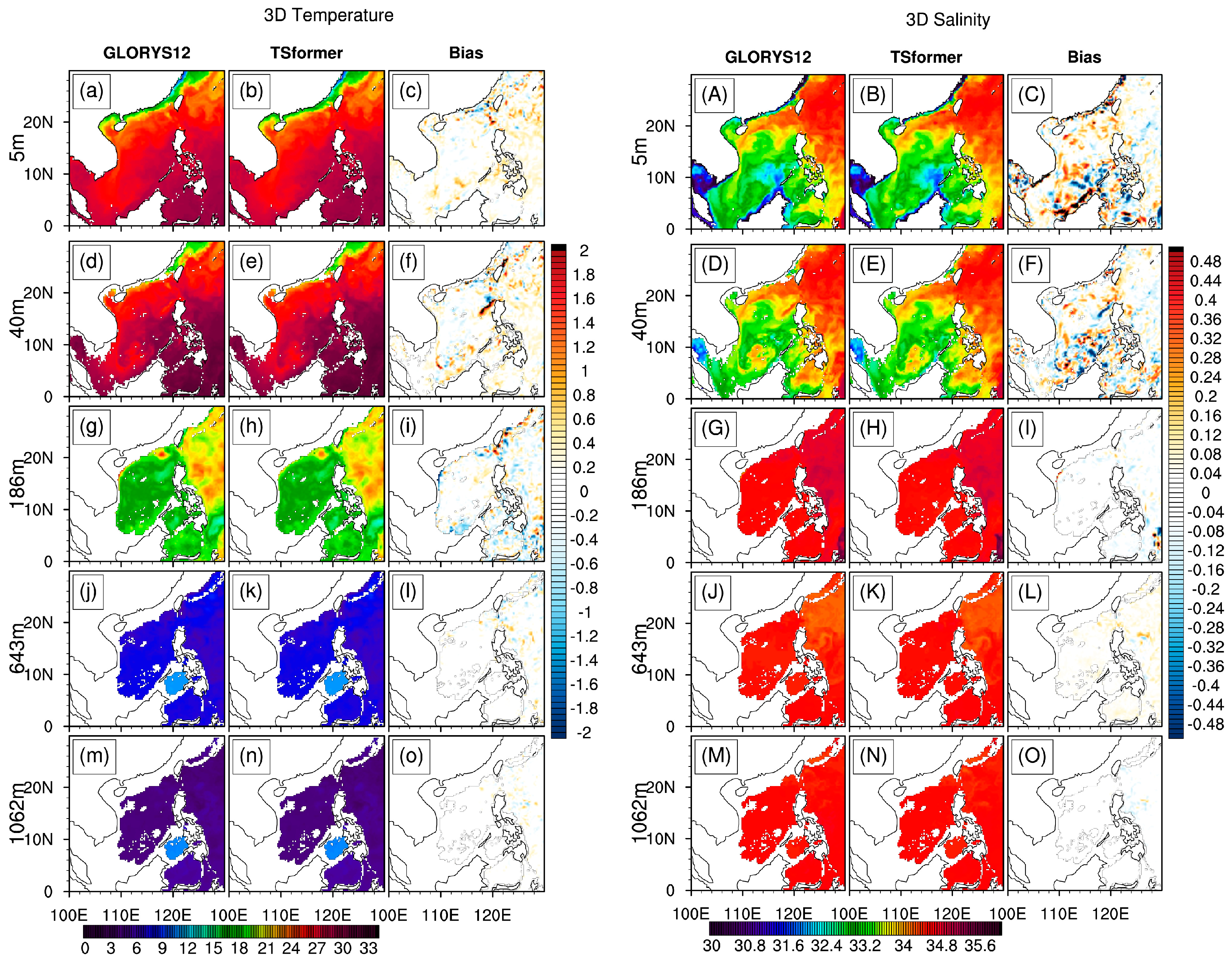
4.2. 3D TS Forecast Results Evaluation with GLORYS12V1

Given that current remote sensing satellites are limited to monitoring only the ocean surface conditions, and with underwater temperature and salinity observations heavily dependent on the sparse data from Argo profiling floats (as referenced in Figure 1), we initially employ the GLORYS12v1 reanalysis data as a benchmark for qualitatively evaluating the accuracy of the TSformer model. Through a comparison of the 3D TS forecasts with the GLORYS12v1 reanalysis dataset (Figure 4), it is observed that the TSformer model accurately captures the characteristics of 3D TS variations at various depths. The spatial distribution of the 3D TS forecast across the mixed layer, thermocline, and deep layer consistently matches the GLORYS12v1 data. Upon analyzing the vertical distribution of biases, temperature biases are primarily concentrated in the thermocline region, while salinity biases are predominantly found in the surface layer, with minimal horizontal biases overall. Specifically, the 3D temperature bias is most pronounced in the Luzon Strait and the eastern sea of the Philippines, regions that are significantly influenced by water mass distribution and seasonal changes due to the Kuroshio [58]. Conversely, the 3D salinity bias is more significant in the northern coastal and southern regions of the SCS, associated with external freshwater inputs and the marine processes driven by the entire SCS monsoon system [59].

Furthermore, it is notable that the TSformer model exhibits intriguing emergent capabilities when trained on a large scale and using non-autoregressive methods. These capabilities enable the TSformer to accurately replicate the physical properties and processes of 3D TS data, which are derived from sequences of physical reanalysis datasets. Impressively, even in the absence of explicit induced biases specific to 3D current fields, the TSformer is capable of generating 3D TS representations that incorporate dynamic current patterns. As the movement of water masses, TS elements consistently flow through 3D space as well.

Figure 5 illustrates the 10-day average of RMSE, MRE, and Bias over time and depth of the 3D TS forecast. The TSformer model displays an average 3D temperature bias of 0.02 °C, maintaining a neutral bias of 0 °C at depths below 250 m. Relative to GLORYS12v1, the TSformer exhibits a warm bias around 30 m, reaching a peak of 0.11 °C (as depicted in Figure 5a), originating from the initial conditions. At the surface, the average 3D temperature RMSE and MRE is 0.45 °C and 1.12%, with the highest RMSE and MRE observed at 80 m (0.60 °C), which subsequently decreases to 0.40 °C at depths below 250 m (Figure 5a). For salinity, the maximum RMSE and MRE is 0.26 PSU and 0.46% at the surface, with an average RMSE of 0.16 PSU above 100 m and 0.04 PSU below 100 m (refer to Figure 5b). The average salinity bias is 0.003 PSU, displaying notable variations with depth.

Figure 6 shows the time series comparison of the 10-day average RMSE and Bias between the TSformer model and the GLORYS12v1 reanalysis data, highlighting the good stability of the TSformer model by comparison. Notably, from July to November 2023, there is a certain increase in the RMSE for both temperature and salinity, coinciding with the active typhoon period in the SCS. This phenomenon will be further discussed in Section 4.4.

Furthermore, we objectively evaluated the skill of the TSformer model with two reference methods: persistence and the TSformer-AR model, which processes discrete single-time-step tokens as inputs and targets. Figure 7 illustrates the detailed quantitative comparison among these three models based on the 2023 operational forecast results against the GLORYS12V1 reanalysis data over the SCS. At lead times of 2 days, the RMSE and ACC of the TSformer-AR are essentially consistent with the TSformer. However, due to its autoregressive methods, the skill of the TSformer-AR declines precipitously beyond 5 cycles, resulting in RMSE values that exceed those of persistence forecasting. Conversely, the TSformer exhibits a gradual and steady increase in the RMSE (or decrease in the ACC), maintaining an ACC above 0.5 for both temperature and salinity by the 30th day. This performance surpasses all baseline models, and demonstrates superior forecasting capabilities. The enhanced performance of the TSformer can be attributed to its end-to-end training for 3D TS forecasting. By employing an efficient space–time attention block and a U-Net encoder–decoder architecture, the TSformer extends the scope of local attention computation from the spatial domain to the spatio-temporal domain. This approach introduces periodic characteristics by expanding the temporal dimension and effectively reduces long-term cumulative errors.

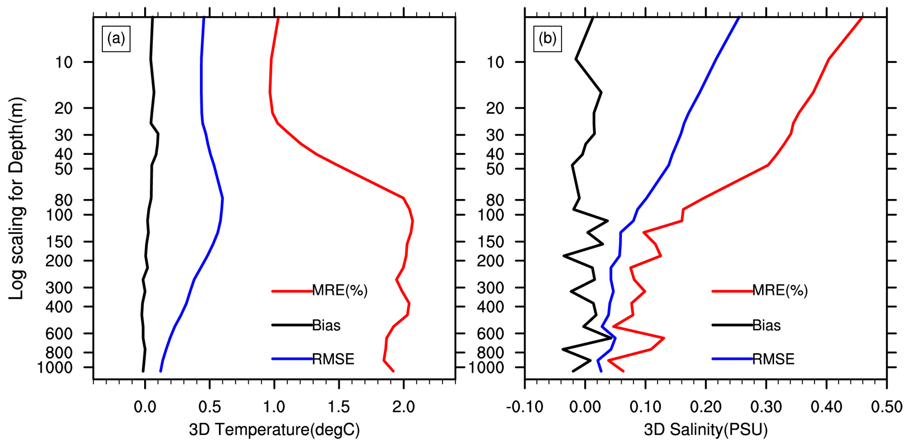
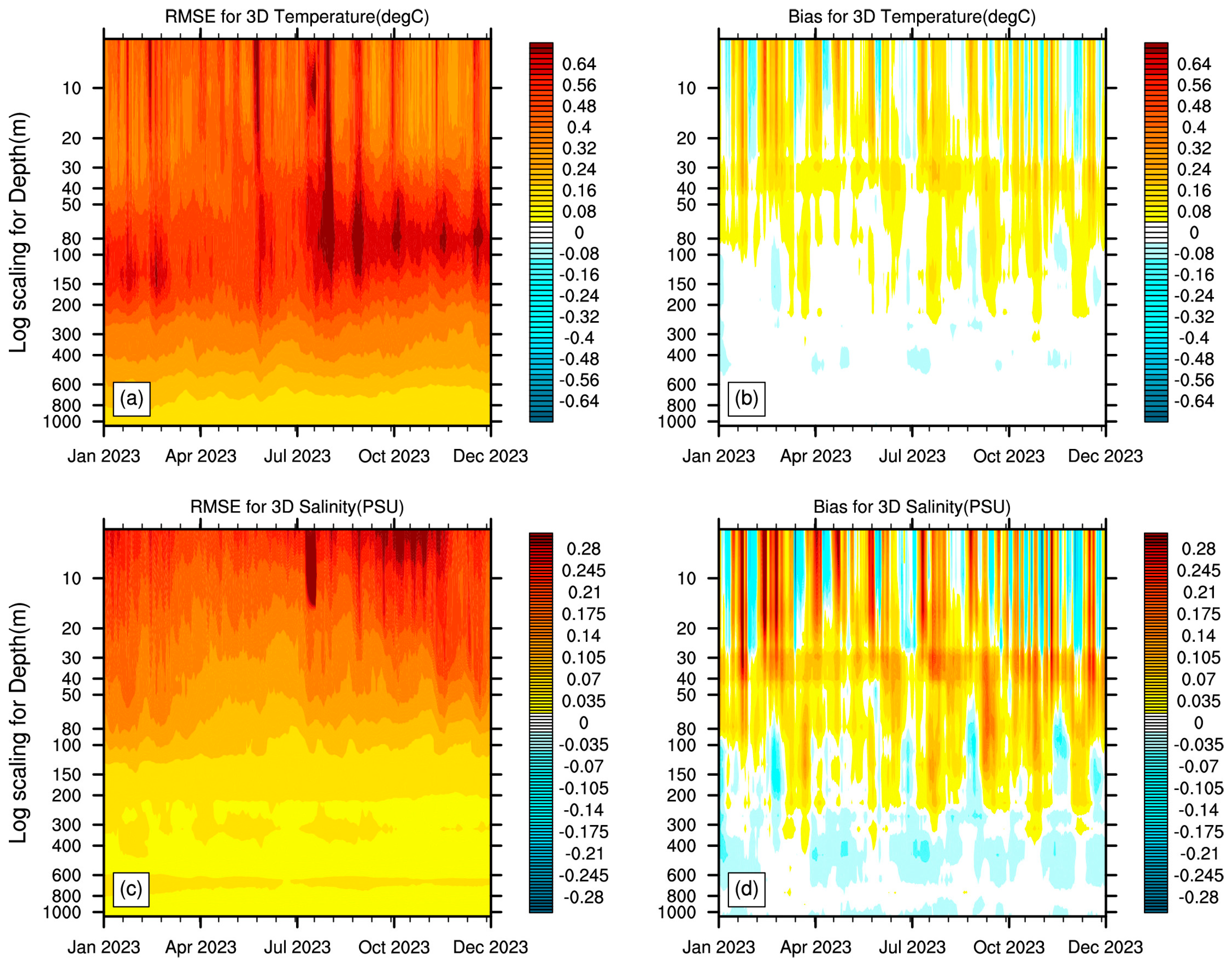
4.3. TS Vertical Profiles Evaluation with Argo

Utilizing the Argo vertical profiles in 2023, the forecasting capability of the TSformer model was evaluated and compared with the state-of-the-art numerical forecasting system PSY4. Figure 8 illustrate the temperature and salinity RMSE profiles for various forecast lead days at depths exceeding 1000 m. It is observed that, within the mixed layer, ranging from 0 to 20 m, the RMSE for the TSformer is slightly higher than that of the PSY4, with an increase that correlates with the forecast lead time. Specifically, on the first lead day, the difference in 3D temperature RMSE between the two models is negligible (less than 0.05 °C), whereas by the 10th lead day, this difference grows to 0.18 °C within the mixed layer. This divergence within the mixed layer may arise from the atmospheric field forcings for the PSY4, which are derived from the ECMWF IFS with a 3-h sampling frequency to capture the diurnal cycle. By contrast, the TSformer currently relies on a daily auxiliary data for surface forcing, which has both significantly larger time and spatial intervals compared to the PSY4. As a result, the TSformer extracts fewer and less comprehensive auxiliary features, leading to increased errors in the surface layer. However, at depths beyond 20 m, the temperature and salinity forecasts from the TSformer significantly surpass those of the PSY4. The average maximum RMSE for temperature is observed at a depth of 50m, with the TSformer reporting values of 0.89 °C and 1.17 °C on the first and tenth days, respectively, compared to the PSY4 values of 1.23 °C and 1.29 °C for the corresponding lead times.

The time series of the area-weighted RMSE, as depicted in Figure 9, indicates that the TSformer model initiates with RMSE values of 0.59 °C for temperature and 0.08 PSU for salinity, both of which are subject to the influence of initial conditions. By the 30th day, these values increase to 0.98 °C and 0.12 PSU, respectively. It is noteworthy that, within the initial 10 days of the forecast, the TSformer model matches the performance of the PSY4 model. Unlike the PSY4, which relies on HPC for extended numerical simulations, the TSformer is capable of completing a 30-day forecast in approximately 40 s utilizing only a CPU, demonstrating a significant advantage in computational efficiency.

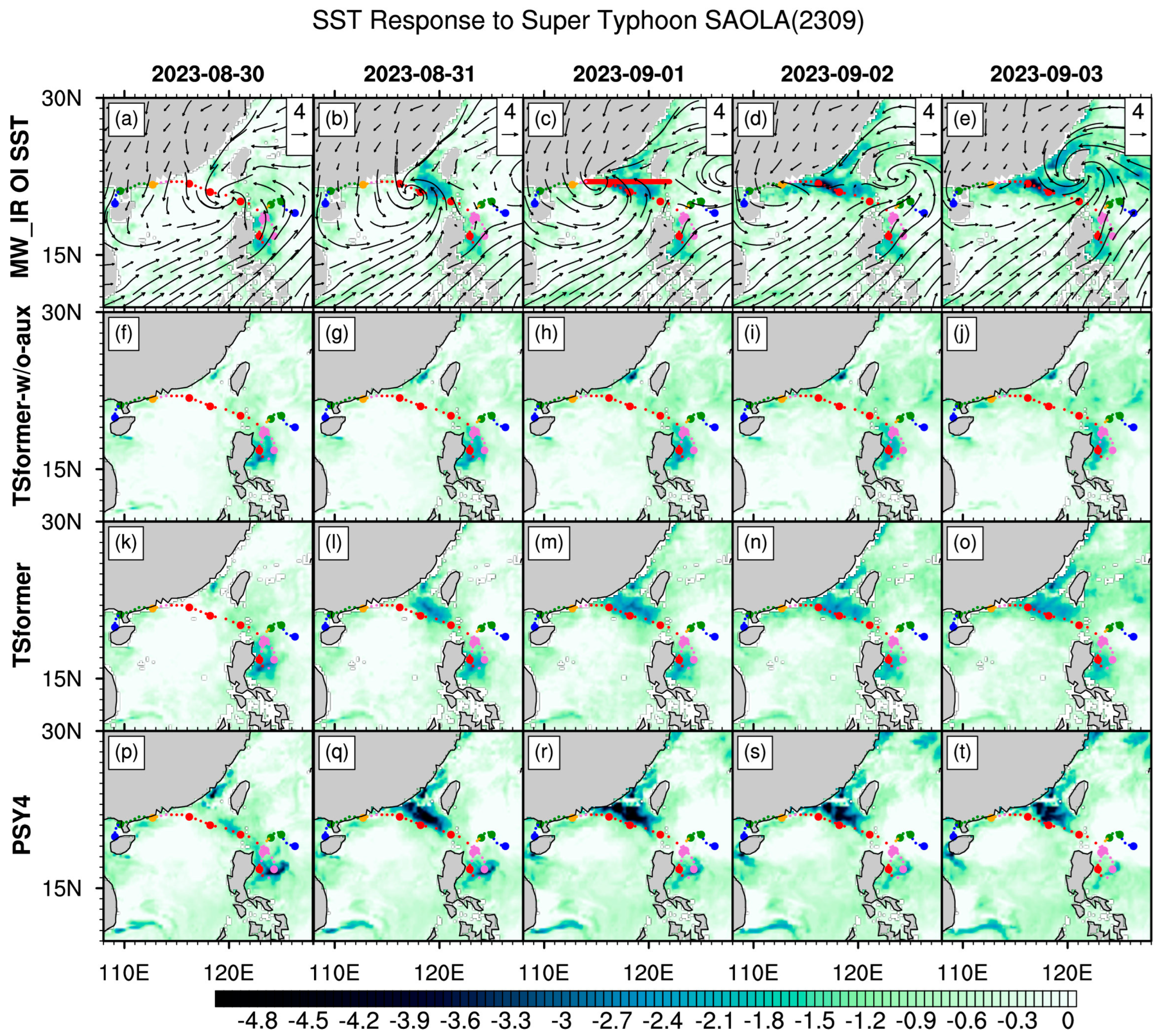
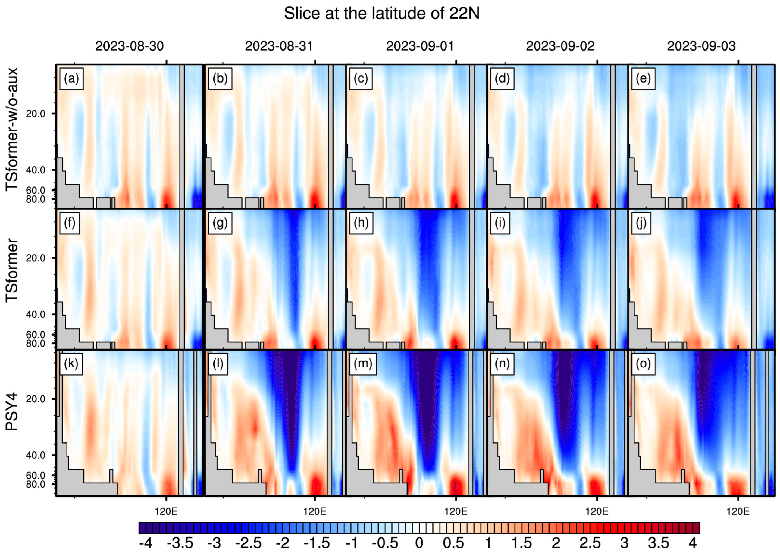
4.4. SST Cooling Evaluation with Satellite Observation

The SCS serves as a critical region for the genesis and landfall of typhoons that originate from the northwest Pacific and the SCS itself [60]. In 2023, the SCS encountered 20 typhoons (Figure 1), with these events typically occurring between April and December. Additionally, with the annual increase in the heat content of the upper ocean, the intensity of typhoons has shown an upward trend over the past forty years [61].

Leveraging the cloud-penetrating capabilities of satellite microwave radiometers, which provide crucial observational data on the SST, this study utilizes the MW_IR OI SST and compares the TSformer model with the PSY4 model and the TSformer model without auxiliary data (TSformer-w/o-aux) to rigorously evaluate the forecast accuracy and stability under typhoon conditions. The time series analysis of the average RMSE and ACC (Figure 10) reveals significant performance differences among the models. Despite utilizing the same 3D TS input data, the TSformer-w/o-aux model, which does not incorporate 2D surface variables as auxiliary input, exhibits lower forecast accuracy for the SST compared to the TSformer and PSY4 models, both in average performance and variability. This divergence is especially marked from May to October, with the TSformer-w/o-aux model exhibiting over a 30% increase in the RMSE for the SST forecasts relative to the TSformer model. Conversely, the TSformer model maintains exceptional stability in the SST forecasting, achieving an average ACC of 0.92 and an average RMSE of 0.50 °C, which is comparable to the performance of the PSY4 model. During the typhoon-active months of July to October, the TSformer model achieves a maximum RMSE of 0.81 °C for the super typhoon Doksuri (2305), outperforming the PSY4 model (1.0 °C).

Tropical cyclones, as intense local disturbances, transfer momentum to the ocean and absorb heat during their movement, leading to significant dynamic and thermal changes in the ocean over a short period [62,63]. These cyclones induce substantial upper-ocean mixing and upwelling, leading to sea surface cooling, thereby producing a negative feedback effect on the cyclone itself [64]. Observations have indicated that the SST cooling caused by tropical cyclone ranges from 1 to 6 °C [65], with a delayed effect, peaking 1–2 days after the cyclone has passed. Notably, this SST cooling exhibits a pronounced asymmetry, primarily related to the forward advection of cold wake water by geostrophic currents on the right side of the cyclone [66].

Taking Super Typhoon Saola (2309) as a case study, we examined the oceanic influences on typhoon-induced SST cooling through the application of three distinct models (Figure 11f–j: TSformer-w/o-aux; Figure 11k–o: TSformer; and Figure 11p–t: PSY4). In this study, the SST cooling is operationally defined by comparing the average SST from 17–20 August 2023 designated as the pre-typhoon baseline (prior to Typhoon Saola, which occurred on 23 August 2023), with the SST values at each grid point from August 30 to September 4. Figure 11a–e illustrate the SST cooling observed by satellite microwave radiometers after the passage of Saola. Saola was classified as a tropical cyclone on August 25 in the eastern waters of Luzon, where it was notably affected by the topography of Luzon Island, which includes elevations surpassing 2000 m. The cyclone lingered in the eastern part of Luzon for four days, resulting in substantial SST cooling (see Figure 11a). On 30 August, Saola crossed the Luzon Strait into the SCS, where the SST were predominantly above 27 °C and exhibited a relatively uniform horizontal distribution. These conditions provided the necessary thermal energy and moisture for the further intensification of the typhoon, leading Saola to rapidly develop into a super typhoon, with the maximum SST cooling amplitude reaching approximately 4.41 °C (see Figure 11b,c). The cooling effects were primarily localized on the right side of the trajectory (see Figure 11c–e). Subsequently, after 2 September, Saola weakened into a tropical cyclone due to friction with the nearshore topography, coinciding with the arrival of Severe Typhoon Haikui (2311) in eastern Taiwan, which caused a decline in the SST in the Taiwan Strait.

Based on the spatial distribution of the SST response to Super Typhoon Saola, the performance of the three models was evaluated (Figure 11). The TSformer-w/o-aux model, which lacks key drivers, such as surface wind fields, inadequately simulated the typhoon-induced SST cooling, with a cooling intensity of only 1.22 °C (see Figure 11i). The TSformer model, which incorporates daily auxiliary input data, accurately predicted the SST cooling characteristics, especially in the region predominantly situated to the right of the track, demonstrating a closer alignment with observational data; however, it underestimated the cooling amplitude, with a recorded intensity of 2.96 °C (Figure 11m). This underestimation might be attributed to the TSformer model current reliance only on auxiliary datasets with larger time and spatial intervals for surface forcing, a limitation discussed in Section 4.3. Conversely, the PSY4 model overestimated the SST cooling intensity, with a value of 6.2 °C (Figure 11r).

Notably, under the initial conditions of a local weak cooling characteristic in the Taiwan Strait (1.14 °C, see Figure 11f,k), both the TSformer-w/o-aux and the TSformer models successfully simulated the SST cooling process induced by the new typhoon Haikui (2311) within the next five days. However, the spatial distribution of the SST cooling forecasted by the TSformer-w/o-aux model was more concentrated, whereas the TSformer model provided a more accurate spatial distribution of the SST cooling, closely matching satellite observations.

Furthermore, the influence of typhoons on the ocean is not limited to the sea surface, they can also impact the subsurface layers of the ocean through mechanisms such as near-inertial oscillations, Ekman pumping, and ocean mixing, with these effects reaching depths of approximately 60 m [67]. Our study focused on the region where the SST cooling was most significant, as indicated by the red line in Figure 11c, and conducted a vertical slice analysis to assess the subsurface impact of typhoons. Upon evaluating the outcomes from the three models (Figure 12), it became clear that the TSformer-w/o-aux model, due to its limited capacity to capture the characteristics of typhoon wind field changes, led to a weaker cooling and slower mixing response. Conversely, the TSformer model, which incorporates surface auxiliary observational data, effectively replicated the vertical cooling and mixing effects induced by Typhoon Saola, achieving a rapid cooling mixing depth of 80 m within a 2-day forecast lead time (Figure 12g). The temporal and spatial distribution patterns of the vertical cooling process from the TSformer model closely matched those of the PSY4 model.

5. Conclusions

In this paper, we explore the large-scale training of an ocean forecast model utilizing the 3D ocean reanalysis product. Specifically, we adopt a hierarchical U-net encoder–decoder architecture, integrated with 3D Swin Transformer blocks, which process spatio-temporal patches of 3D TS variables and 2D surface forcing. Our target model, the TSformer, is capable of forecasting 30 days of 3D eddy-resolving ocean physical variables in a non-autoregressive approach, with a daily temporal resolution and a 1/12° spatial resolution that covers 3D TS variables across 26 vertical levels.

The performance of the TSformer model has been comprehensively evaluated through its comparison with the GLORYS12V1 reanalysis data and verification against data from the Argo profiling floats and satellite observations. Based on the near-real-time operational forecast results from 2023, the TSformer, which differs from autoregressive models, has expanded the scope of local attention computation from the spatial to the spatio-temporal. This expansion not only preserves the consistency of 3D TS in the physical motion process within space but maintains long-range coherence and stability in long-term forecasts, significantly reducing cumulative errors. Moreover, the TSformer model jointly extracts both 3D TS features and 2D surface forcing characteristics through its 3D Swin Transformer modules, which are adept at handling self-attention computations in parallel at the cubic level. As a result, the TSformer has demonstrated its effectiveness in managing extreme events, exemplified by its successful forecasting of the SST cooling induced by Super Typhoon Saola. It is particularly remarkable that the TSformer has outperformed the PSY4 model in forecasting the thermocline dynamics below a depth of 20 m in the SCS, a critical factor for enhancing our comprehension of the internal structure and processes of the oceans. Specifically, the TSformer model is capable of completing a comprehensive 30-day forecast in approximately 40 s using only CPU resources, which is significantly faster by orders of magnitude compared to traditional numerical forecast models.

While the TSformer model offers computational efficiency and high accuracy in ocean eddy-resolving forecasting, there is room for enhancement. The first limitation is that TSformer relies on 2D daily remote sensing data for surface forcing, omitting essential parameters at the air–sea interface, such as air temperature, pressure, fluxes, and precipitation. This deficiency limits the ability to fully simulate vertical and horizontal exchanges and interactions, leading to weaker typhoon-induced cooling. To address this, future iterations of the TSformer model could integrate a broader spectrum of weather parameters with ERA5 atmospheric reanalysis datasets, and increase the capability of resolving fine-scale processes with high-resolution satellite observations (e.g., the Surface Water and Ocean Topography mission). The second limitation is that the deterministic nature of the TSformer limits its capacity to provide probabilistic forecasts and uncertainties, especially over extended forecast periods. Enhancing the TSformer to include probabilistic forecasting could mitigate these limitations by offering a spectrum of potential outcomes and their probabilities. This would enable the model to present multiple future scenarios, thereby enhancing the forecast capabilities for extreme events. By incorporating these improvements, the TSformer could achieve a more comprehensive and nuanced understanding of complex atmospheric and oceanic phenomena, ultimately refining its forecasting prowess.

References

1. Suthers, I.M.; Young, J.W.; Baird, M.E.; Roughan, M.; Everett, J.D.; Brassington, G.B.; Byrne, M.; Condie, S.A.; Hartog, J.R.; Hassler, C.S.; et al. The Strengthening East Australian Current, Its Eddies and Biological Effects—An Introduction and Overview. Deep. Res. Part II Top. Stud. Oceanogr. 2011, 58, 538–546. [Google Scholar] [CrossRef]
2. Cheng, L.; Abraham, J.; Hausfather, Z.; Trenberth, K. How Fast Are the Oceans Warming? Science 2019, 363, 128–129. [Google Scholar] [CrossRef]
3. Fox-Kemper, B.; Hewitt, H.T.; Xiao, C.; Aðalgeirsdóttir, G.; Drijfhout, S.S.; Edwards, T.L.; Golledge, N.R.; Hemer, M.; Kopp, R.E.; Krinner, G. Ocean, Cryosphere and Sea Level Change. Climate Change 2021: The Physical Science Basis. Contribution of Working Group I to the Sixth Assessment Report of the Intergovernmental Panel on Climate Change; Zhai, P., Pirani, A., Eds.; IPCC: Geneva, Switzerland, 2021. [Google Scholar]
4. Liu, X.; Wang, Y.; Zhang, H.; Guo, X. Susceptibility of Typical Marine Geological Disasters: An Overview. Geoenviron. Disasters 2023, 10, 10. [Google Scholar] [CrossRef]
5. Burnet, W.; Harper, S.; Preller, R.; Jacobs, G.; Lacroix, K. Overview of Operational Ocean Forecasting in the US Navy: Past, Present, and Future. Oceanography 2014, 27, 24–31. [Google Scholar] [CrossRef]
6. Blockley, E.W.; Martin, M.J.; McLaren, A.J.; Ryan, A.G.; Waters, J.; Lea, D.J.; Mirouze, I.; Peterson, K.A.; Sellar, A.; Storkey, D. Recent Development of the Met Office Operational Ocean Forecasting System: An Overview and Assessment of the New Global FOAM Forecasts. Geosci. Model Dev. 2014, 7, 2613–2638. [Google Scholar] [CrossRef]
7. Semtner, A.J., Jr.; Chervin, R.M. A Simulation of the Global Ocean Circulation with Resolved Eddies. J. Geophys. Res. Ocean. 1988, 93, 15502–15522. [Google Scholar] [CrossRef]
8. Gurvan, M.; NEMO Team. NEMO Ocean Engine (Version v3.6). 2017, p. 1472492. Available online: https://epic.awi.de/id/eprint/39698/1/NEMO_book_v6039.pdf (accessed on 10 May 2025).
9. Guo, H.; Chen, Z.; Zhu, R.; Cai, J. Increasing Model Resolution Improves but Overestimates Global Mid-Depth Circulation Simulation. Sci. Rep. 2024, 14, 29356. [Google Scholar] [CrossRef]
10. Zhang, S.; Fu, H.; Wu, L.; Li, Y.; Wang, H.; Zeng, Y.; Duan, X.; Wan, W.; Wang, L.; Zhuang, Y.; et al. Optimizing High-Resolution Community Earth System Model on a Heterogeneous Many-Core Supercomputing Platform. Geosci. Model Dev. 2020, 13, 4809–4829. [Google Scholar] [CrossRef]
11. Xiao, B.; Qiao, F.; Shu, Q.; Yin, X.; Wang, G.; Wang, S. Development and Validation of a Global 1∕32° Surface-Wave–Tide–Circulation Coupled Ocean Model: FIO-COM32. Geosci. Model Dev. 2023, 16, 1755–1777. [Google Scholar] [CrossRef]
12. Li, X.; Liu, B.; Zheng, G.; Ren, Y.; Zhang, S.; Liu, Y.; Gao, L.; Liu, Y.; Zhang, B.; Wang, F. Deep-Learning-Based Information Mining from Ocean Remote-Sensing Imagery. Natl. Sci. Rev. 2021, 7, 1584–1605. [Google Scholar] [CrossRef]
13. Ravuri, S.; Lenc, K.; Willson, M.; Kangin, D.; Lam, R.; Mirowski, P.; Fitzsimons, M.; Athanassiadou, M.; Kashem, S.; Madge, S.; et al. Skilful Precipitation Nowcasting Using Deep Generative Models of Radar. Nature 2021, 597, 672–677. [Google Scholar] [CrossRef] [PubMed]
14. Zhang, Y.; Long, M.; Chen, K.; Xing, L.; Jin, R.; Jordan, M.I.; Wang, J. Skilful Nowcasting of Extreme Precipitation with NowcastNet. Nature 2023, 619, 526–532. [Google Scholar] [CrossRef]
15. Berbić, J.; Ocvirk, E.; Carević, D.; Lončar, G. Application of Neural Networks and Support Vector Machine for Significant Wave Height Prediction. Oceanologia 2017, 59, 331–349. [Google Scholar] [CrossRef]
16. Wolff, S.; O’Donncha, F.; Chen, B. Statistical and Machine Learning Ensemble Modelling to Forecast Sea Surface Temperature. J. Mar. Syst. 2020, 208, 103347. [Google Scholar] [CrossRef]
17. Weyn, J.A.; Durran, D.R.; Caruana, R.; Cresswell-Clay, N. Sub-seasonal Forecasting with a Large Ensemble of Deep-learning Weather Prediction Models. J. Adv. Model. Earth Syst. 2021, 13, e2021MS002502. [Google Scholar] [CrossRef]
18. Ham, Y.G.; Kim, J.H.; Luo, J.J. Deep Learning for Multi-Year ENSO Forecasts. Nature 2019, 573, 568–572. [Google Scholar] [CrossRef]
19. Ashkezari, M.D.; Hill, C.N.; Follett, C.N.; Forget, G.; Follows, M.J. Oceanic Eddy Detection and Lifetime Forecast Using Machine Learning Methods. Geophys. Res. Lett. 2016, 43, 12234–12241. [Google Scholar] [CrossRef]
20. Shi, X.; Chen, Z.; Wang, H.; Yeung, D.Y.; Wong, W.K.; Woo, W.C. Convolutional LSTM Network: A Machine Learning Approach for Precipitation Nowcasting. In Proceedings of the Advances in Neural Information Processing Systems, Montreal, QC, Canada, 7–12 December 2015; pp. 802–810. [Google Scholar]
21. Wang, Y.; Jiang, L.; Yang, M.H.; Li, L.J.; Long, M.; Fei-Fei, L. Eidetic 3D LSTM: A Model for Video Prediction and Beyond. In Proceedings of the 7th International Conference on Learning Representations, ICLR 2019, New Orleans, LA, USA, 6–9 May 2019; p. 10. [Google Scholar]
22. Xiao, C.; Tong, X.; Li, D.; Chen, X.; Yang, Q.; Xv, X.; Lin, H.; Huang, M. Prediction of Long Lead Monthly Three-Dimensional Ocean Temperature Using Time Series Gridded Argo Data and a Deep Learning Method. Int. J. Appl. Earth Obs. Geoinf. 2022, 112, 102971. [Google Scholar] [CrossRef]
23. Wang, G.; Wang, X.; Wu, X.; Liu, K.; Qi, Y.; Sun, C.; Fu, H. Hybrid Multivariate Deep Learning Network for Multistep Ahead Sea Level Anomaly Forecasting. J. Atmos. Ocean. Technol. 2022, 39, 285–301. [Google Scholar] [CrossRef]
24. Dong, C.; Xu, G.; Han, G.; Bethel, B.J.; Xie, W.; Zhou, S. Recent Developments in Artificial Intelligence in Oceanography. Ocean. Res. 2022, 2022, 9870950. [Google Scholar] [CrossRef]
25. Vaswani, A.; Shazeer, N.; Parmar, N.; Uszkoreit, J.; Jones, L.; Gomez, A.N.; Kaiser, Ł.; Polosukhin, I. Attention Is All You Need. Adv. Neural Inf. Process. Syst. 2017, 30, 5998–6008. [Google Scholar]
26. Dosovitskiy, A.; Beyer, L.; Kolesnikov, A.; Weissenborn, D.; Zhai, X.; Unterthiner, T.; Dehghani, M.; Minderer, M.; Heigold, G.; Gelly, S.; et al. An Image Is Worth 16X16 Words: Transformers for Image Recognition At Scale. In Proceedings of the ICLR 2021—9th International Conference on Learning Representations, Virtual, 3–7 May 2021. [Google Scholar]
27. Han, T.; Guo, S.; Ling, F.; Chen, K.; Gong, J.; Luo, J.; Gu, J.; Dai, K.; Ouyang, W.; Bai, L. Fengwu-Ghr: Learning the Kilometer-Scale Medium-Range Global Weather Forecasting. arXiv 2024, arXiv:2402.00059. [Google Scholar]
28. Kurth, T.; Subramanian, S.; Harrington, P.; Pathak, J.; Mardani, M.; Hall, D.; Miele, A.; Kashinath, K.; Anandkumar, A. Fourcastnet: Accelerating Global High-Resolution Weather Forecasting Using Adaptive Fourier Neural Operators. In Proceedings of the Platform for Advanced Scientific Computing Conference, Davos, Switzerland, 26–28 June 2023; pp. 1–11. [Google Scholar]
29. Lam, R.; Sanchez-Gonzalez, A.; Willson, M.; Wirnsberger, P.; Fortunato, M.; Alet, F.; Ravuri, S.; Ewalds, T.; Eaton-Rosen, Z.; Hu, W.; et al. Learning Skillful Medium-Range Global Weather Forecasting. Science 2023, 382, 1416–1421. [Google Scholar] [CrossRef] [PubMed]
30. Bi, K.; Xie, L.; Zhang, H.; Chen, X.; Gu, X.; Tian, Q. Accurate Medium-Range Global Weather Forecasting with 3D Neural Networks. Nature 2023, 619, 533–538. [Google Scholar] [CrossRef] [PubMed]
31. Liu, Z.; Lin, Y.; Cao, Y.; Hu, H.; Wei, Y.; Zhang, Z.; Lin, S.; Guo, B. Swin Transformer: Hierarchical Vision Transformer Using Shifted Windows. In Proceedings of the IEEE International Conference on Computer Vision, Montreal, QC, Canada, 11–17 October 2021; pp. 9992–10002. [Google Scholar]
32. Gao, Z.; Shi, X.; Wang, H.; Zhu, Y.; Wang, Y.B.; Li, M.; Yeung, D.-Y. Earthformer: Exploring Space-Time Transformers for Earth System Forecasting. Adv. Neural Inf. Process. Syst. 2022, 35, 25390–25403. [Google Scholar]
33. Liu, Z.; Hu, H.; Lin, Y.; Yao, Z.; Xie, Z.; Wei, Y.; Ning, J.; Cao, Y.; Zhang, Z.; Dong, L.; et al. Swin Transformer V2: Scaling Up Capacity and Resolution. In Proceedings of the IEEE Computer Society Conference on Computer Vision and Pattern Recognition, New Orleans, LA, USA, 18–24 June 2022; pp. 11999–12009. [Google Scholar]
34. Chen, L.; Zhong, X.; Zhang, F.; Cheng, Y.; Xu, Y.; Qi, Y.; Li, H. FuXi: A Cascade Machine Learning Forecasting System for 15-Day Global Weather Forecast. npj Clim. Atmos. Sci. 2023, 6, 190. [Google Scholar] [CrossRef]
35. Chen, L.; Zhong, X.; Li, H.; Wu, J.; Lu, B.; Chen, D.; Xie, S.-P.; Wu, L.; Chao, Q.; Lin, C.; et al. A Machine Learning Model That Outperforms Conventional Global Subseasonal Forecast Models. Nat. Commun. 2024, 15, 6425. [Google Scholar] [CrossRef]
36. Wang, X.; Wang, R.; Hu, N.; Wang, P.; Huo, P.; Wang, G.; Wang, H.; Wang, S.; Zhu, J.; Xu, J. Xihe: A Data-Driven Model for Global Ocean Eddy-Resolving Forecasting. arXiv 2024, arXiv:2402.02995. [Google Scholar]
37. Patrick, M.; Campbell, D.; Asano, Y.; Misra, I.; Metze, F.; Feichtenhofer, C.; Vedaldi, A.; Henriques, J.F. Keeping Your Eye on the Ball: Trajectory Attention in Video Transformers. Adv. Neural Inf. Process. Syst. 2021, 34, 12493–12506. [Google Scholar]
38. Fan, H.; Xiong, B.; Mangalam, K.; Li, Y.; Yan, Z.; Malik, J.; Feichtenhofer, C. Multiscale Vision Transformers. In Proceedings of the IEEE/CVF International Conference on Computer Vision, Montreal, BC, Canada, 11–17 October 2021; pp. 6824–6835. [Google Scholar]
39. Yan, S.; Xiong, X.; Arnab, A.; Lu, Z.; Zhang, M.; Sun, C.; Schmid, C. Multiview Transformers for Video Recognition. In Proceedings of the IEEE/CVF Conference on Computer Vision and Pattern Recognition, New Orleans, LA, USA, 18–24 June 2022; pp. 3333–3343. [Google Scholar]
40. Jean-Michel, L.; Eric, G.; Romain, B.-B.; Gilles, G.; Angélique, M.; Marie, D.; Clément, B. The Copernicus Global 1/12 Oceanic and Sea Ice GLORYS12 Reanalysis. Front. Earth Sci. 2021, 9, 698876. [Google Scholar] [CrossRef]
41. Mears, C.; Lee, T.; Ricciardulli, L.; Wang, X.; Wentz, F. Improving the Accuracy of the Cross-Calibrated Multi-Platform (CCMP) Ocean Vector Winds. Remote Sens. 2022, 14, 4230. [Google Scholar] [CrossRef]
42. Good, S.; Fiedler, E.; Mao, C.; Martin, M.J.; Maycock, A.; Reid, R.; Roberts-Jones, J.; Searle, T.; Waters, J.; While, J.; et al. The Current Configuration of the OSTIA System for Operational Production of Foundation Sea Surface Temperature and Ice Concentration Analyses. Remote Sens. 2020, 12, 720. [Google Scholar] [CrossRef]
43. Wong, A.P.S.; Wijffels, S.E.; Riser, S.C.; Pouliquen, S.; Hosoda, S.; Roemmich, D.; Gilson, J.; Johnson, G.C.; Martini, K.; Murphy, D.J.; et al. Argo Data 1999–2019: Two Million Temperature-Salinity Profiles and Subsurface Velocity Observations From a Global Array of Profiling Floats. Front. Mar. Sci. 2020, 7, 700. [Google Scholar] [CrossRef]
44. Chao, G.; Wu, X.; Zhang, L.; Fu, H.; Liu, K.; Han, G. China Ocean ReAnalysis (CORA) Version 1.0 Products and Validation for 2009–18. Atmos. Ocean. Sci. Lett. 2021, 14, 100023. [Google Scholar] [CrossRef]
45. Sun, W.; Wang, J.; Zhang, J.; Ma, Y.; Meng, J.; Yang, L.; Miao, J. A New Global Gridded Sea Surface Temperature Product Constructed from Infrared and Microwave Radiometer Data Using the Optimum Interpolation Method. Acta Oceanol. Sin. 2018, 37, 41–49. [Google Scholar] [CrossRef]
46. Wang, X.; Wang, C.; Han, G.; Li, W.; Wu, X. Effects of Tropical Cyclones on Large-Scale Circulation and Ocean Heat Transport in the South China Sea. Clim. Dyn. 2014, 43, 3351–3366. [Google Scholar] [CrossRef]
47. Tuo, P.; Yu, J.Y.; Hu, J. The Changing Influences of ENSO and the Pacific Meridional Mode on Mesoscale Eddies in the South China Sea. J. Clim. 2018, 32, 685–700. [Google Scholar] [CrossRef]
48. Liu, Z.; Ning, J.; Cao, Y.; Wei, Y.; Zhang, Z.; Lin, S.; Hu, H. Video Swin Transformer. In Proceedings of the IEEE Computer Society Conference on Computer Vision and Pattern Recognition, New Orleans, LA, USA, 18–24 June 2022; pp. 3192–3201. [Google Scholar]
49. Courtier, P.; Thépaut, J.-N.; Hollingsworth, A. A Strategy for Operational Implementation of 4D-Var, Using an Incremental Approach. Q. J. R. Meteorol. Soc. 1994, 120, 1367–1387. [Google Scholar] [CrossRef]
50. Xiao, Y.; Bai, L.; Xue, W.; Chen, K.; Han, T.; Ouyang, W. FengWu-4DVar: Coupling the Data-Driven Weather Forecasting Model with 4D Variational Assimilation. arXiv 2023, arXiv:2312.12455. [Google Scholar]
51. Dee, D.P.; Uppala, S.M.; Simmons, A.J.; Berrisford, P.; Poli, P.; Kobayashi, S.; Andrae, U.; Balmaseda, M.A.; Balsamo, G.; Bauer, P.; et al. The ERA-Interim Reanalysis: Configuration and Performance of the Data Assimilation System. Q. J. R. Meteorol. Soc. 2011, 137, 553–597. [Google Scholar] [CrossRef]
52. Lorenc, A.C.; Rawlins, F. Why Does 4D-Var Beat 3D-Var? Q. J. R. Meteorol. Soc. A J. Atmos. Sci. Appl. Meteorol. Phys. Oceanogr. 2005, 131, 3247–3257. [Google Scholar] [CrossRef]
53. Llugsi, R.; El Yacoubi, S.; Fontaine, A.; Lupera, P. Comparison between Adam, AdaMax and Adam W Optimizers to Implement a Weather Forecast Based on Neural Networks for the Andean City of Quito. In Proceedings of the 2021 IEEE Fifth Ecuador Technical Chapters Meeting (ETCM), Cuenca, Ecuador, 12–15 October 2021; IEEE: Piscataway, NJ, USA, 2021; pp. 1–6. [Google Scholar]
54. Zhao, Y.; Gu, A.; Varma, R.; Luo, L.; Huang, C.-C.; Xu, M.; Wright, L.; Shojanazeri, H.; Ott, M.; Shleifer, S.; et al. Pytorch Fsdp: Experiences on Scaling Fully Sharded Data Parallel. arXiv 2023, arXiv:2304.11277. [Google Scholar] [CrossRef]
55. Lellouche, J.M.; Greiner, E.; Le Galloudec, O.; Garric, G.; Regnier, C.; Drevillon, M.; Benkiran, M.; Testut, C.E.; Bourdalle-Badie, R.; Gasparin, F.; et al. Recent Updates to the Copernicus Marine Service Global Ocean Monitoring and Forecasting Real-Time 1 g 12° High-Resolution System. Ocean Sci. 2018, 14, 1093–1126. [Google Scholar] [CrossRef]
56. Levine, R.A.; Wilks, D.S. Statistical Methods in the Atmospheric Sciences. J. Am. Stat. Assoc. 2000, 95, 344. [Google Scholar] [CrossRef]
57. Shriver, J.F.; Hurlburt, H.E.; Smedstad, O.M.; Wallcraft, A.J.; Rhodes, R.C. 1/32° Real-Time Global Ocean Prediction and Value-Added Over 1/16° Resolution. J. Mar. Syst. 2007, 65, 3–26. [Google Scholar] [CrossRef]
58. Qu, T. Upper-Layer Circulation in the South China Sea. J. Phys. Oceanogr. 2000, 30, 1450–1460. [Google Scholar] [CrossRef]
59. Yi, D.L.; Melnichenko, O.; Hacker, P.; Potemra, J. Remote Sensing of Sea Surface Salinity Variability in the South China Sea. J. Geophys. Res. Ocean. 2020, 125, e2020JC016827. [Google Scholar] [CrossRef]
60. Zhao, Z.; Yang, S.; Wang, H.; Yuan, T.; Ren, K. The Remote Effects of Typhoons on the Cold Filaments in the Southwestern South China Sea. Remote Sens. 2024, 16, 3293. [Google Scholar] [CrossRef]
61. Guan, S.; Li, S.; Hou, Y.; Hu, P.; Liu, Z.; Feng, J. Increasing Threat of Landfalling Typhoons in the Western North Pacific Between 1974 and 2013. Int. J. Appl. Earth Observ. Geoinf. 2018, 68, 279–286. [Google Scholar] [CrossRef]
62. Potter, H.; Drennan, W.M.; Graber, H.C. Upper Ocean Cooling and Air-Sea Fluxes Under Typhoons: A Case Study. J. Geophys. Res. Ocean. 2017, 122, 7237–7252. [Google Scholar] [CrossRef]
63. Wang, X.D.; Han, G.J.; Qi, Y.Q.; Li, W. Impact of Barrier Layer on Typhoon-Induced Sea Surface Cooling. Dyn. Atmos. Ocean. 2011, 52, 367–385. [Google Scholar] [CrossRef]
64. Jullien, S.; Marchesiello, P.; Menkes, C.E.; Lefèvre, J.; Jourdain, N.C.; Samson, G.; Lengaigne, M. Ocean Feedback to Tropical Cyclones: Climatology and Processes. Clim. Dyn. 2014, 43, 2831–2854. [Google Scholar] [CrossRef]
65. Bender, M.A.; Ginis, I.; Kurihara, Y. Numerical Simulations of Tropical Cyclone-ocean Interaction with a High-resolution Coupled Model. J. Geophys. Res. Atmos. 1993, 98, 23245–23263. [Google Scholar] [CrossRef]
66. Vincent, E.M.; Lengaigne, M.; Vialard, J.; Madec, G.; Jourdain, N.C.; Masson, S. Assessing the Oceanic Control on the Amplitude of Sea Surface Cooling Induced by Tropical Cyclones. J. Geophys. Res. Ocean. 2012, 117, C5. [Google Scholar] [CrossRef]
67. Karnauskas, K.B.; Zhang, L.; Emanuel, K.A. The Feedback of Cold Wakes on Tropical Cyclones. Geophys. Res. Lett. 2021, 48, e2020GL091676. [Google Scholar] [CrossRef]
Figure 1. The launch location of the 941 Argo floats (yellow points) under delayed mode quality control in the South China Sea (SCS) for the year 2023. The black lines indicate the paths of the 20 typhoons that affected the SCS in 2023.
Jmse 13 00966 g001
Figure 2. An overview of the proposed TSformer model architecture.
Jmse 13 00966 g002
Figure 3. An illustration of two successive 3D Swin Transformer block.
Jmse 13 00966 g003
Figure 4. A Visualization example of the spatial distribution of forecast performance on 5 January 2023. The forecasts generated by the TSformer model for the fifth day (starting from 1 January 2023) are depicted in the second and fifth columns, whereas the GLORYS12V1 reanalysis data is shown in the first and fourth columns. Additionally, the figure includes a spatial map illustrating the bias between the TSformer and GLORYS12V1 for 3D Temperature (third column) and 3D Salinity (sixth column). (ao) 3D Temperature (AO) 3D Salinity.
Jmse 13 00966 g004
Figure 5. The 10-day average RMSE (blue line), MRE (red line), and Bias (black line) profiles for the 3D temperature (a) and 3D salinity (b), respectively.
Jmse 13 00966 g005
Figure 6. The time series comparison of the 10-day average RMSE and Bias for the TSformer model and the GLORYS12v1 reanalysis is presented. (a) RMSE for 3D temperature (b) Bias for 3D temperature (c) RMSE for 3D salinity (d) Bias for 3D salinity.
Jmse 13 00966 g006
Figure 7. The forecast skill comparison of the average RMSE (black line) and ACC (blue line) based on the 2023 operational forecast results against the GLORYS12V1 reanalysis data over the SCS for both 3D temperature (a) and 3D salinity (b).
Jmse 13 00966 g007
Figure 8. The vertical profiles of the average RMSE for 3D temperature (a) and 3D salinity (b), as compared with Argo data for two different models: the TSformer (solid line) and the PSY4 (dashed line). The lead times for the forecasts are represented by different colors: 1 day (blue), 10 days (orange), and 30 days (red).
Jmse 13 00966 g008
Figure 9. The forecast performance of the average RMSE for 3D temperature (red) and 3D salinity (blue), respectively, as compared with Argo data for two different models: the TSformer (solid line) and the PSY4 (dashed line).
Jmse 13 00966 g009
Figure 10. The time series comparison of the 3-day average RMSE (a) and ACC (b) of the SST forecast is depicted for the TSformer-w/o-aux (red), the TSformer (blue), and the PSY4 (black). These evaluations are benchmarked against the MW_IR OI SST dataset, with both sets of results extracted from the 2023 operational forecast results.
Jmse 13 00966 g010
Figure 11. The oceanic influences on typhoon-induced cooling, as observed through the MW_IR OI SST (panels (ae)) and assessed using three distinct models (panels (fj): TSformer-w/o-aux, panels (ko): TSformer, and panels (pt): PSY4).
Jmse 13 00966 g011
Figure 12. The impact of Typhoon Saola on the subsurface ocean layers at the latitude of 22N, where the SST cooling effect was most pronounced. The study presents the results from three models: TSformer-w/o-aux (panels (ae)), TSformer (panels (fj)), and PSY4 (panels (ko)).
Jmse 13 00966 g012