Synergistic Effects of Ocean Background and Tropical Cyclone Characteristics on Tropical Cyclone-Induced Sea Surface Cooling in the Western North Pacific

Abstract

Tropical cyclones (TCs) induce intense mixing in the upper ocean, which significantly impacts sea surface temperature (SST) and marine environment. Previous studies have shown that TCs can cause a decrease in sea surface temperature (DSST), while further research is required to elucidate the factors influencing SST changes. This study employs satellite observations and reanalysis data from the western North Pacific during 2002–2020 to investigate the relationship between DSST and the ocean background state (BG). In addition, by incorporating TC characteristics, we construct indices to explore the synergistic effects of TCs and BG on DSST, enabling a more comprehensive understanding of the mechanisms governing DSST variability. The results indicate that DSST exhibits significant monthly variations, with the maximum DSST in September for coastal regions and in August for offshore regions. Regardless of TC characteristics, when the mixed layer depth (MLD) exceeds 60 m or thermocline depth (TD) exceeds 115 m, it is difficult for the DSST to exceed 1 °C. In both coastal and offshore regions, MLD and TD exhibit moderate negative correlations with DSST, with values around −0.3. When TC characteristics are incorporated, these correlations rise to approximately 0.6, highlighting the importance of jointly considering BG and TC effects in characterizing DSST. The findings of this study provide theoretical support for improving the capability to predict DSST changes before the TC approaches the coast.

1. Introduction

Tropical cyclones (TCs) are frequent natural hazards in the Western North Pacific (WNP) during the summer [1], causing widespread destruction in coastal regions through intense winds and large waves [2]. TCs are closely coupled with oceanic conditions, exhibiting strong interactions [3,4,5,6]. A sea surface temperature (SST) above 26 °C provides the energy required for TC intensification [7,8,9], and SST largely determines the maximum potential intensity a TC can reach. Conversely, stronger TCs induce a greater decrease in sea surface temperature (DSST) along their tracks [1,10,11,12]. In addition to TCs, the ocean background state (BG) can also affect DSST; therefore, studying the synergistic effects of TCs and BG on DSST is essential [13,14,15,16,17,18]. Furthermore, since coastal and offshore regions exhibit different ocean structures, it is necessary to investigate DSST in each region separately.

During the passage period of TCs, DSST is primarily driven by dynamic processes, including strong wind-driven vertical mixing of cold subsurface water and upwelling [19,20,21,22,23]. In offshore regions, vertical mixing plays a dominant role, whereas in coastal regions, advection processes play a primary role [24,25]. In contrast, thermal processes such as heat exchange contribute less than 20% to DSST [26,27,28]. The dynamic and thermal factors inducing DSST are both influenced by the TCs and BG characteristics. For instance, slow-moving, intense TCs generally cause greater DSST than fast-moving, weaker TCs [29,30,31,32,33,34]. Additionally, Pun et al. [32] demonstrated that when TCs curve northward along their tracks, both TC size and the average radius of maximum wind increase significantly, thereby sustaining the intensity of DSST. Previous studies have emphasized the importance of TC characteristics in influencing DSST. For example, Pun et al. [35] reported moderate correlations between DSST and parameters such as TC size, intensity, and translation speed. Vincent et al. [12] proposed the Wind Power Index to quantify DSST based on TC forcing, while Cui et al. [36] applied machine learning to identify intensity, size, and speed as key predictors. In addition to TC characteristics, the upper ocean vertical structure also plays a key role in TC-induced mixing [37].

Since vertical mixing depends strongly on the vertical temperature structure, the degree of DSST is closely linked to pre-existing stratification [11,38]. Moreover, when TCs are weaker, faster-moving, or smaller, they induce less intense and shallower mixing, allowing the stratified temperature profile to exert an increasingly dominant influence on DSST [35,39,40,41,42,43,44]. Mixed layer depth (MLD) and thermocline depth (TD) are key indicators of the vertical temperature profile. MLD refers to the depth of the upper ocean layer with relatively uniform temperature and salinity, while TD represents the depth at which the ocean temperature decreases most rapidly with depth. Previous studies have indicated that shallow MLD and TD facilitate the entrainment of colder subsurface waters by wind-driven mixing and upwelling, resulting in a significant DSST. Conversely, when the entrainment is limited, DSST is substantially suppressed [45,46,47,48,49,50]. Furthermore, freshwater enhances the ocean’s salinity stratification, which fosters the formation of a barrier layer at the base of the mixed layer. When TCs pass through the barrier layer region, this layer suppresses the vertical mixing and DSST induced by TCs [51,52,53]. Moreover, research by Miles et al. [54] shows that the suppression of DSST can reach up to 57%. Additionally, in the Bay of Bengal, the DSST during the pre-monsoon season is approximately three times that after the monsoon season. This difference is essentially related to seasonal changes in oceanic stratification rather than to differences in TC wind energy input. During the post-monsoon season, stronger thermal stratification and significant upper-ocean freshening strongly inhibit DSST induced by vertical mixing beneath TCs. On average, thermal stratification contributes to 60% of this cooling reduction during postmonsoon season, while haline stratification contributes to the remaining 40% [55,56]. Previous studies have highlighted the role of ocean background conditions in DSST. For instance, Da et al. [24] and Vincent et al. [56] demonstrated the importance of stratification metrics like MLD and SST–T100, while Oey [57] proposed a nonlinear model capturing upper-ocean structure. However, these parameters are often examined in isolation from TC characteristics, limiting an integrated understanding.

Many studies have investigated TC-induced DSST in both coastal and offshore regions. Observational and numerical simulation research has revealed significant differences in the characteristics of BG between these areas, resulting in distinct oceanic responses to TCs [15,17,25,33,58]. To further explore how the distinct structural characteristics of coastal and offshore regions influence TC-induced DSST, this study divided the WNP into these two regions to examine the spatial and temporal distribution of the BG and DSST, as well as their correlation, and further explore the synergistic effects of the TC and BG on DSST, proposing indices to better characterize DSST. This study provides an understanding of TC-induced ocean cooling, offering both new perspectives on ocean–atmosphere interactions and a theoretical foundation for improving TC forecasts and early warning systems in coastal regions.

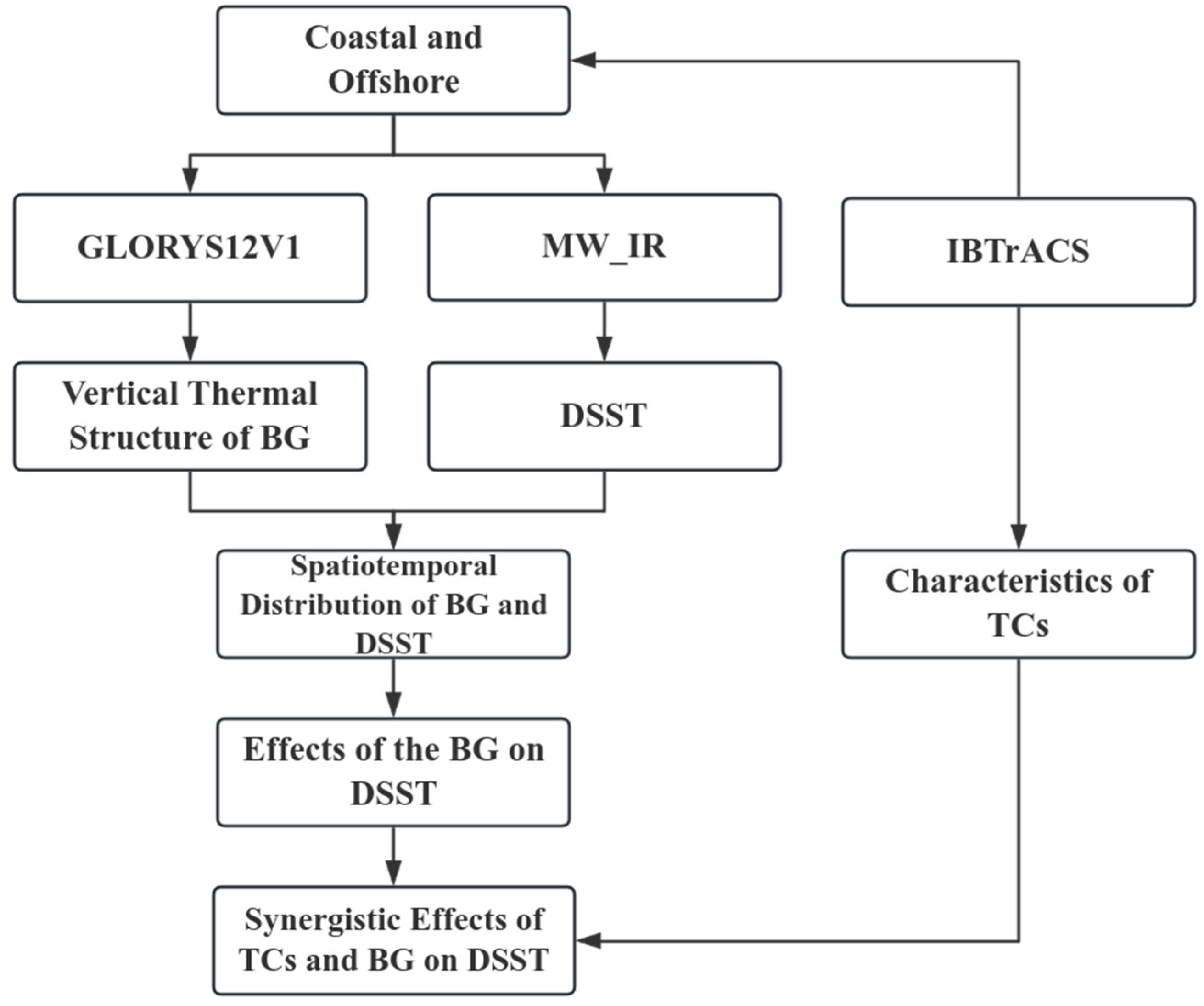
2. Materials and Methods

2.1. Data

TC data are obtained from Version 4 [59] of the International Best Track Archive for Climate Stewardship (IBTrACS), accessed through the NOAA National Centers for Environmental Information. This dataset includes a range of TC characteristic parameters with 3-h temporal resolution, where each interval represents a distinct observation. Hereafter, the term ‘observation’ refers to a record in the IBTrACS dataset corresponding to a specific 3-h interval. The dataset includes the TCs’ geographic coordinates, maximum sustained wind speed (usa_wind in the dataset, MW hereafter for short), translation speed of the TC (storm_speed in the dataset, Trans hereafter for short), radius of 34-knot winds (usa_r34 in the dataset, R34 hereafter for short), and other relevant parameters used to represent the characteristics of TCs. Da et al. [24] demonstrated notable variations in TC and BG within and beyond 500 km from the coastlines. The vertical temperature gradient remains stable in regions within 500 km from the coastline before declining, while the salinity gradient (MLD) decreases (increases) rapidly, and then changes at a slower rate. Beyond 500 km offshore, MW gradually decreases, Trans gradually increases, and R34 remains steady, while these parameters show pronounced variability within 500 km. Building on this finding, this study partitions the WNP into coastal and offshore regions using a 500 km threshold from continental and major island coastlines. Specifically, any TC observations with a distance-to-land (dist2land) value ≤ 500 km are classified as coastal regions, while those > 500 km are designated offshore regions.

For the computation of DSST, we use the satellite sea surface temperature dataset (MW_IR), which integrates microwave and infrared remote sensing data provided by Remote Sensing Systems. The spatial resolution of the dataset is $0.25°\times 0.25°$ from June 2002 to now and this daily dataset is less affected by clouds [60].

Subsurface temperature is derived from the GLORYS12V1 [61] reanalysis product (GLOBAL_MULTIYEAR_PHY_001_030), obtained through the Copernicus Marine Environment Monitoring Service (CMEMS). This eddy-resolving dataset provides daily 3D temperature fields from 1993 to present, spanning 50 vertical levels (0–5500 m) with 1/12° horizontal resolution, thus fully meeting the requirements of this study to calculate relevant parameters of the vertical temperature structure in the BG. In addition, previous studies have shown that GLORYS12V1 is consistent with observed ocean temperatures, as it assimilates Argo float data and exhibits good agreement with Argo profiles, with a maximum difference of less than 0.2 °C and a root mean square (RMS) error of 0.02 °C [62]. All data used cover the period from June 2002 to the end of 2020.

2.2. Methods

After the passage of a TC, more than 40% of the DSST recovers to the climatological SST within 5 days [8]. In addition, the average R34 of a TC is approximately 300 km [35], and Yu et al. [63] found that SST decreases were observed at 86% of locations within a 300 km radius from the TC center. Based on these considerations, for each TC observation in this study, DSST is defined as the difference between the SST for the post-TC period (averaged over 1–5 days after the TC) and the pre-TC period (averaged over 1–5 days before the TC). The regional mean SST difference is calculated within a $6°\times 6°$ area centered on the TC location.

For the BG, this study calculates the vertical temperature structure of a $6°\times 6°$ sea area centered on the TC location 5 days prior to the TC. Given that strong TCs typically induce mixing within the upper 100 m, this study adopts the temperature at 100 m (T100) as a key parameter. It also utilizes temperature difference between the SST and T100, denoted as SST-T100 [56], which effectively captures the extent of DSST associated with upper mixing processes.

To comprehensively explain the effect of the BG on DSST and considering the vertical mixing-induced cooling, this study defines the MLD using a temperature threshold method that captures the vertical temperature structure. A threshold of 0.8 °C is adopted, as it is applicable across global oceans and in all seasons. Compared with other thresholds, 0.8 °C can accurately represent the penetration depth of turbulent mixing [64]. In addition to mixed layer, we also consider the thermocline. To characterize the ocean vertical thermal structure and its influence on DSST, this study adopts thermocline parameters—including thermocline thickness (T Thickness), TD, and thermocline strength (TS)—following the definitions and calculation methods proposed by Fiedler [65]. These parameters provide a physically meaningful description of the thermocline based on established stratification metrics, ensuring consistency with previous studies.

The first parameter, T Thickness is defined as the vertical distance between the thermocline bottom (TB) and MLD:

$$\mathrm{T}\mathrm{Thickness}=\mathrm{TB}-\mathrm{MLD}$$

(1)

where TB is defined as the depth at which temperature equals the midpoint between the mixed layer temperature (MLT) and T400. T400 is the temperature at 400 m [65]. The region beneath 400 m exhibits a relatively steady vertical temperature gradient largely insensitive to seasonal or regional variability, whereas the MLD shows pronounced seasonal variation. Since the thermocline lies between a seasonally variable upper layer and a relatively stable deep layer, this stratification-based approach provides a consistent and adaptable method for identifying TB across different oceanic regions and seasons.

The second parameter, TD, is defined as the midpoint between the MLD and the TB, approximating the location of the steepest temperature gradient within the thermocline. Compared with previous studies that adopted a fixed isotherm (e.g., 20 °C or 12 °C) to represent thermocline depth, we follow Fiedler‘s [65] approach by using a location-dependent definition of TD. This method better captures spatial and temporal variability in thermocline structure, and reflects the physical transition zone between the seasonally varying upper ocean and the more stable deep layer. TD is calculated as follows:

$$\mathrm{TD}=(\mathrm{MLD}+\mathrm{TB})\times 0.5$$

(2)

The third parameter, TS, is defined to quantify the intensity of the thermocline, representing the temperature gradient between the thermocline temperature (TT) and the MLT over the depth range between the TD and MLD, calculated as follows:

$$\mathrm{TS}={\displaystyle \frac{\mathrm{TT}-\mathrm{MLT}}{\mathrm{TD}-\mathrm{MLD}}}$$

(3)

where MLT represents the temperature at the MLD, and TT is calculated as follows:

$$\mathrm{TT}=\mathrm{MLT}-0.25\times (\mathrm{MLT}-\mathrm{T}400)$$

(4)

TT is the temperature at the midpoint between MLT and TB temperature, which can be approximated as the temperature at the location of the steepest decline. Equation (4) presents its simplified form.

Six ocean thermal parameters (T100, SST-T100, MLD, T Thickness, TD and TS) are calculated to describe the spatial and temporal differences in the BG and to analyze the impact of the BG on the magnitude of the DSST in the WNP. Additionally, for each TC observation, a $6°\times 6°$ grid was interpolated centered on the TC center. After gridding, only grid cells with at least five TC observations were retained for analysis to ensure statistical robustness. In addition, months with insufficient TC occurrences were excluded from the annual analysis. The main abbreviations used in this study are listed in

Table 1. List of abbreviations and their corresponding full terms used throughout this study.

Abbreviation	Full Term	Abbreviation	Full Term
BG	Ocean Background State	TB	Thermocline Bottom
DSST	Decrease in Sea Surface Temperature	TC	Tropical Cyclone
MLD	Mixed Layer Depth	TD	Thermocline Depth
MLT	Mix Layer Temperature	Trans	Translation Speed of TC
MW	Maximum Sustained Wind Speed	TS	Thermocline Strength
R34	Radius of 34-knot Winds	TT	Thermocline Temperature
SST	Sea Surface Temperature	T Thickness	Thermocline Thickness
T100	Temperature at 100 m	WNP	Western North Pacific

.

Overall, this study uses the GLORYS12V1 dataset to calculate the vertical thermal structure of the BG and the MW_IR dataset to calculate DSST. This study then statistically analyzes the spatiotemporal distributions of BG and DSST. TC characteristics are derived from the IBTrACS dataset to study the synergistic effects of TCs and BG on DSST. Additionally, the distance-to-land from the IBTrACS dataset is used to distinguish between coastal and offshore TCs, with a 500 km threshold from the coastline (Figure 1).

3. Results

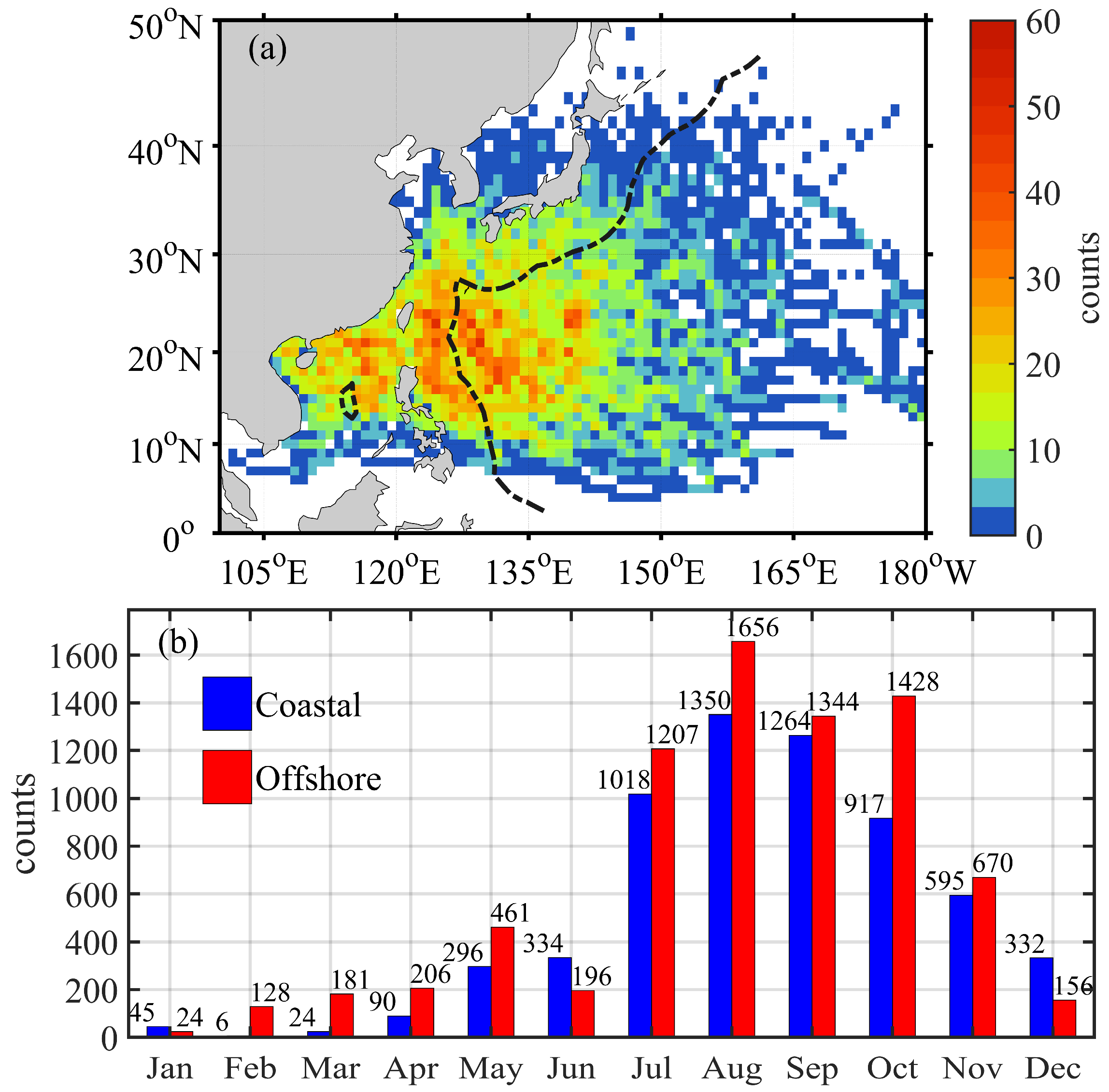
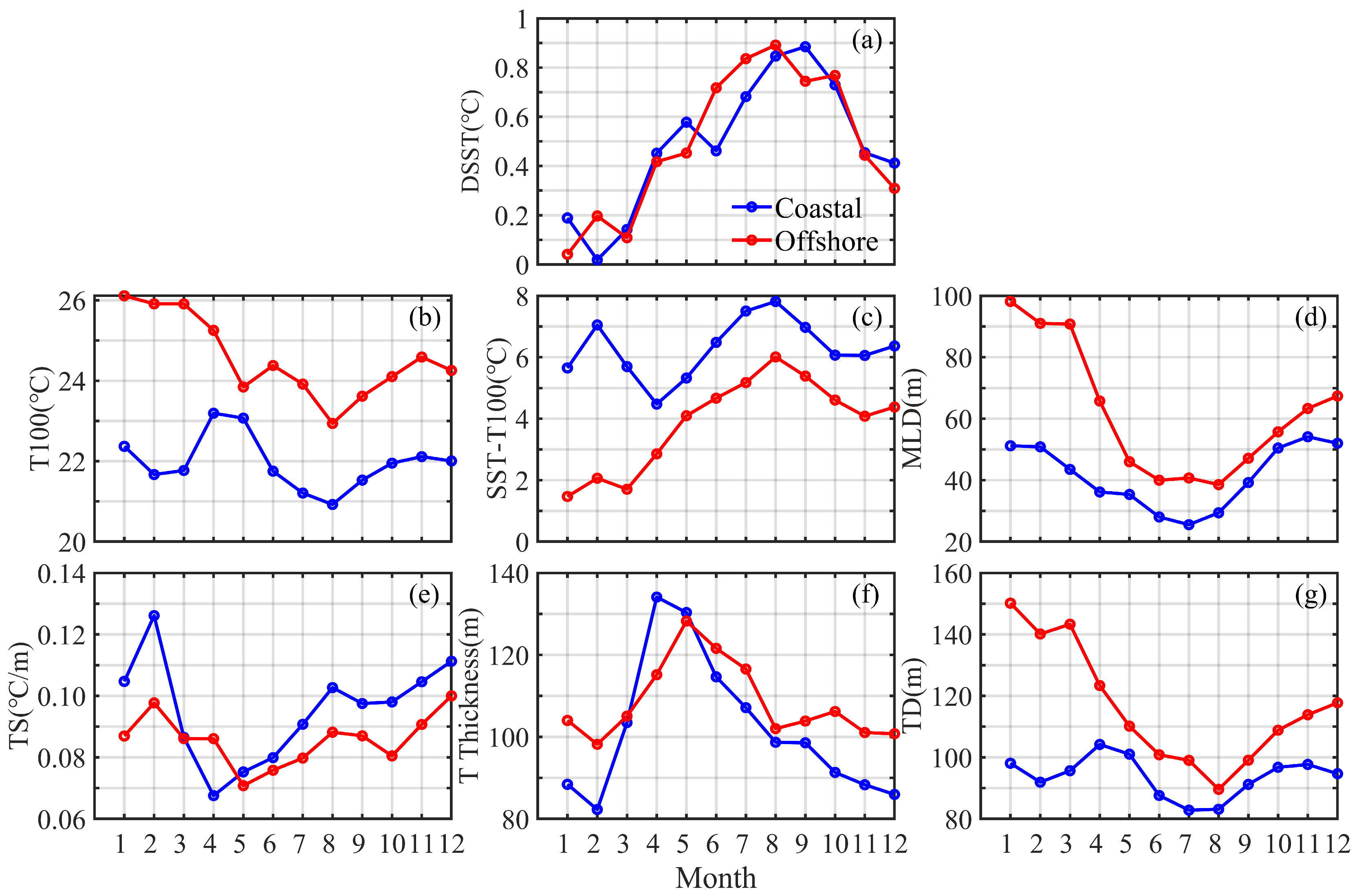
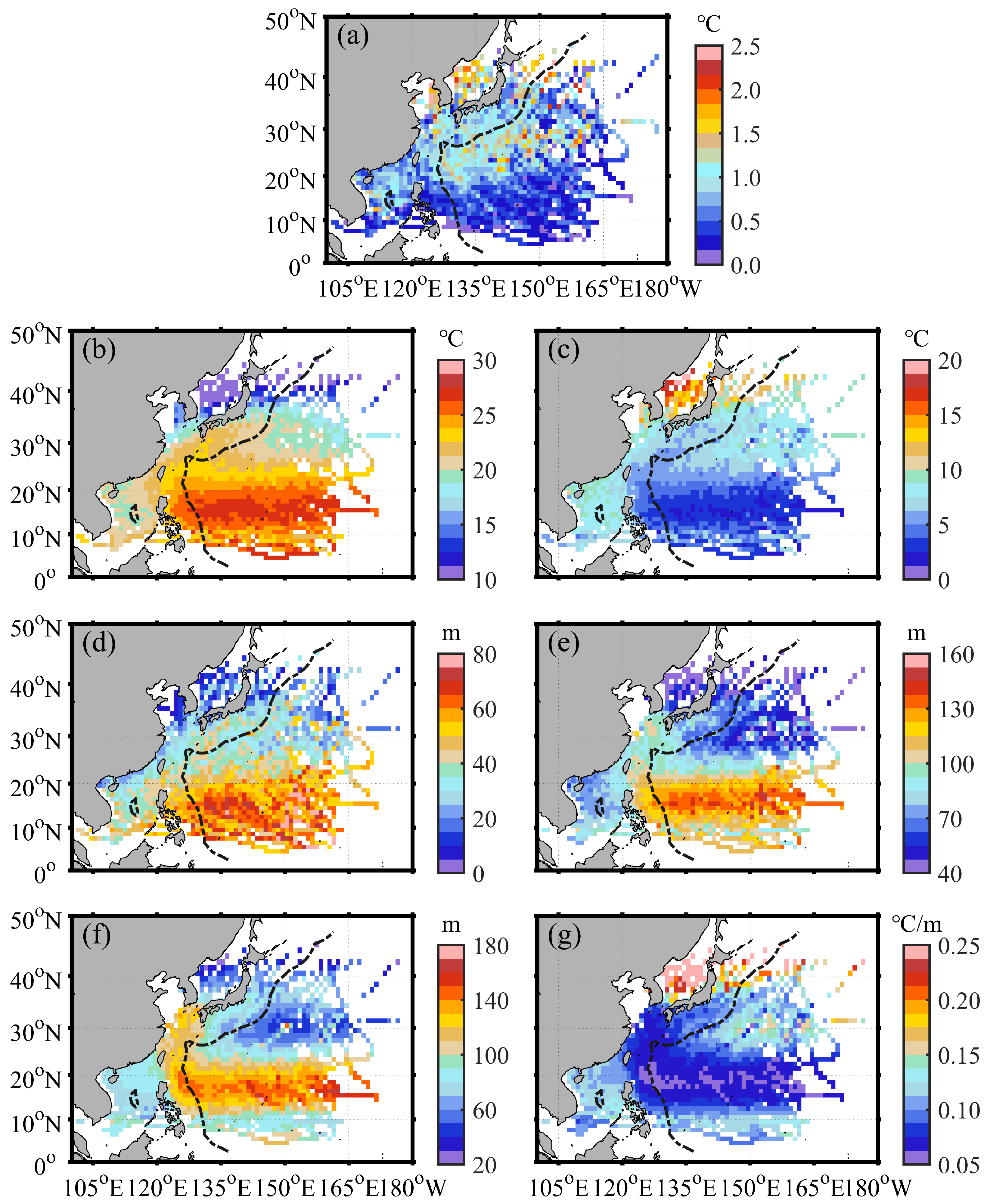
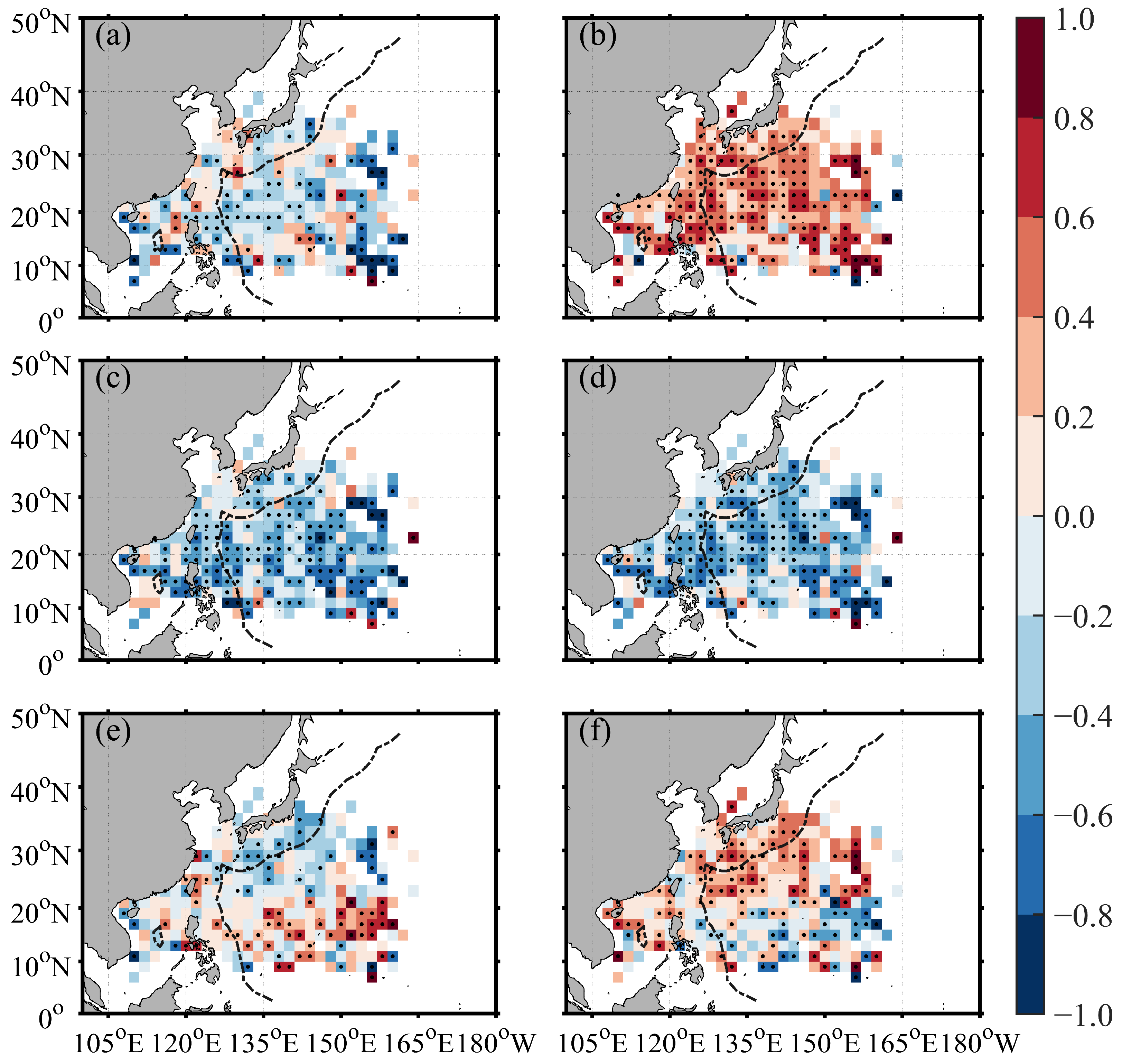
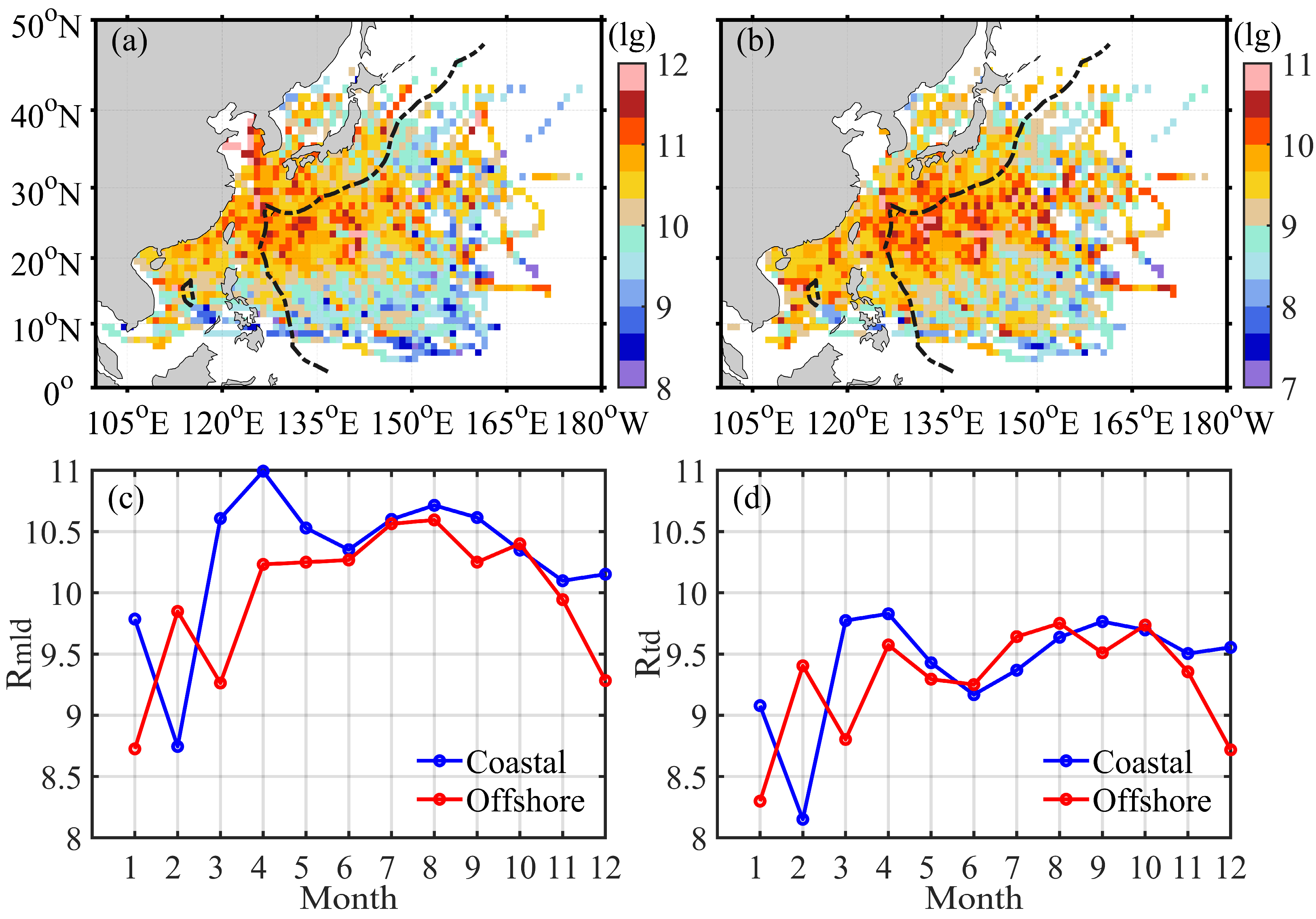
3.1. Spatial and Temporal Distribution of BG and DSST in the WNP

This study compiles the number of TCs and the number of TC observations in the WNP. Figure 2a reveals pronounced TC clustering in the WNP, mainly concentrated to the west of 140° E between 15° N and 30° N. The highest concentration is near Luzon Island (16° N, 121° E) and decreases outward. During the study period, a total of 376 TCs are recorded. The total number of TC observations in the coastal regions amounted to 6271, while the offshore regions accounted for 7657. The monthly distribution demonstrates strong seasonality, with 73% of coastal region and 74% of offshore region TC occurrences concentrated in July–October, and the highest concentration observed in August. Conversely, January–March accounts for <3% of annual activity, which may have a certain impact on the results of the subsequent analysis (Figure 2b).

The number of TCs exhibits a pronounced seasonal variability. Therefore, this study analyzes the monthly variations of different BG parameters in the WNP. As shown in Figure 3, the climatological monthly variations reveal significant coastal–offshore contrasts in the BG parameters. During the months with a large number of TCs (July–October), the DSST exceeds 0.6 $°\mathrm{C}$, with the maximum exceeding 0.85 $°\mathrm{C}$ in September for coastal regions and in August for offshore regions (Figure 2b and Figure 3a). T100 reaches its minimum in August, with the coastal minimum approaching 21 $°\mathrm{C}$ and offshore minimum approaching 23 $°\mathrm{C}$, which is even comparable to the coastal maximum in April (Figure 3b). SST-T100 reaches its annual maximum in August, indicating that the vertical temperature gradient between the surface and 100 m depth is conducive to amplifying the DSST induced by TCs (Figure 3c). The MLD and TD generally exhibit a V-shaped distribution, with minimum values occurring in summer, and offshore regions are consistently higher than those in coastal regions across all months. Specifically, the MLD (TD) minimum value is about 25 m (80 m) in coastal regions and about 38 m (90 m) in offshore regions (Figure 3d,g). TS and T Thickness exhibit opposite temporal trends from April to December, with TS demonstrating an increasing trend while T Thickness shows a decreasing trend (Figure 3e,f).

Additionally, this study focuses on the climatological spatial distribution of various BG parameters in the WNP. As shown in Figure 4, the spatial pattern of the DSST exhibits a latitudinal gradient, with stronger cooling in the northern regions and lower cooling in the southern regions. This pattern corresponds to the distribution of SST-T100, which generally decreases toward the south, whereas T100 exhibits the opposite trend (Figure 4a–c). In the north of 20° N, shallower MLD and TD enhance cooling, whereas deeper MLD and TD in the south of 20° N are associated with weaker cooling (Figure 4a,d,e). Both T Thickness and TS reach their maximum and minimum values between 10° N and 20° N, and their distribution patterns exhibit some differences compared to DSST (Figure 4a,f,g).

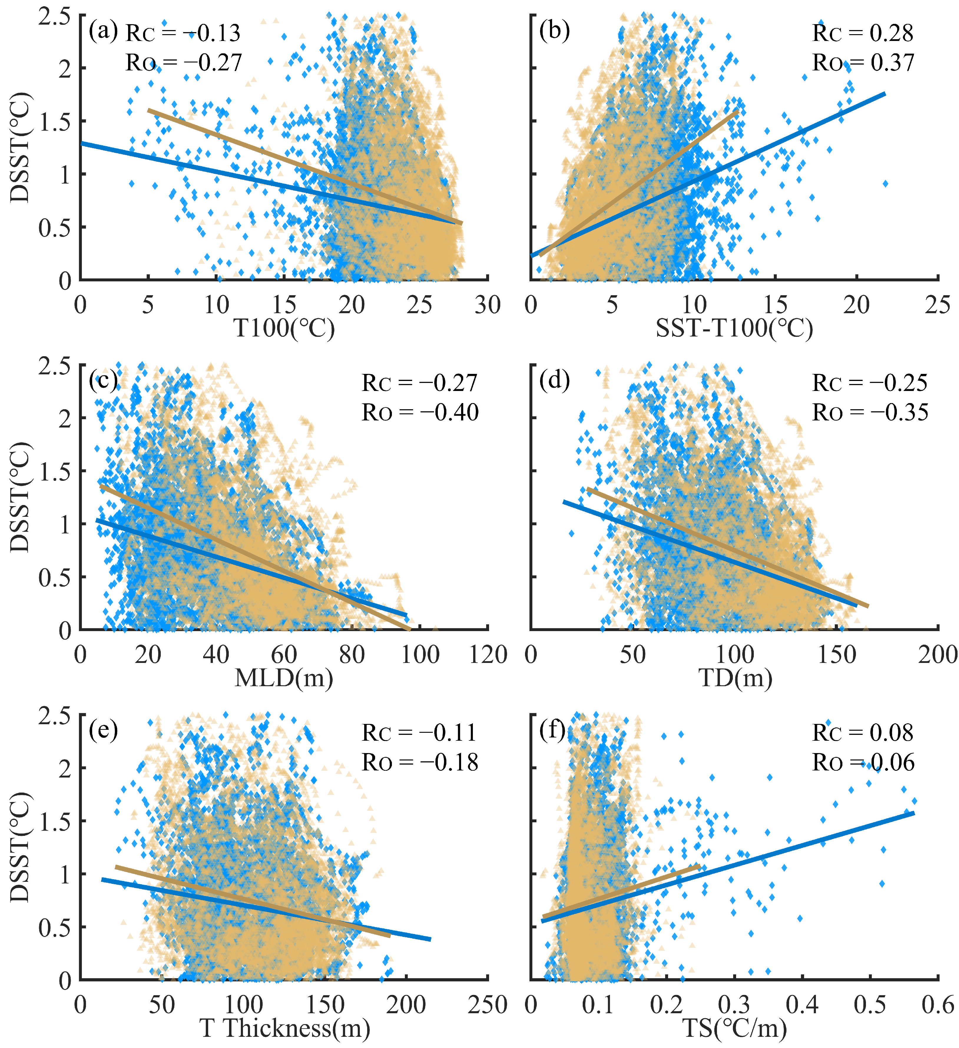
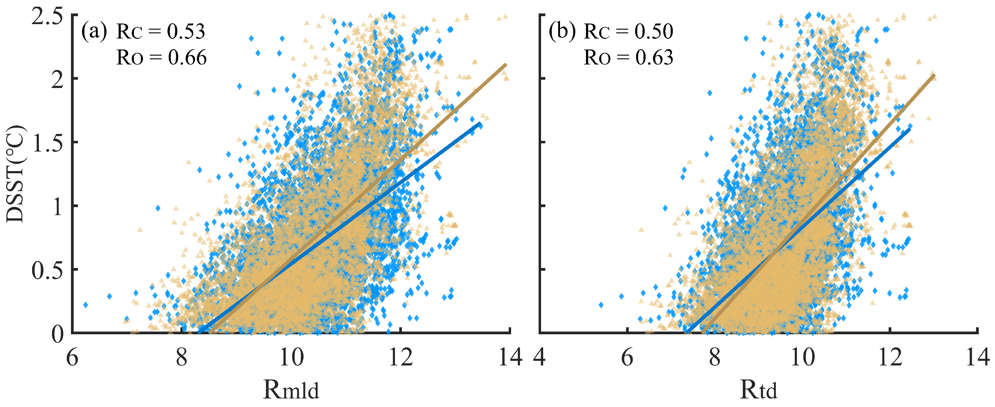
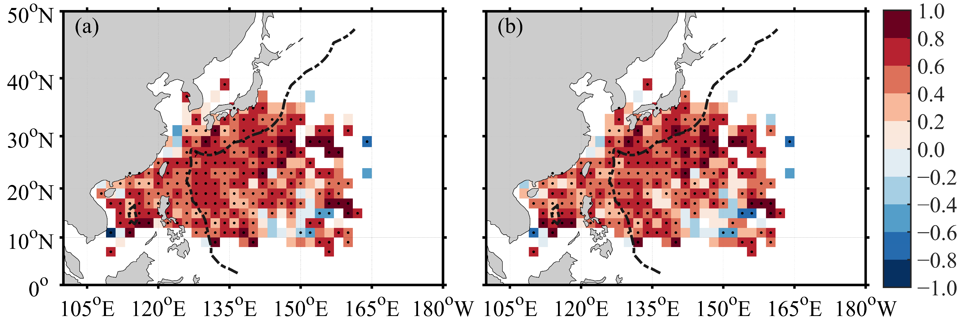
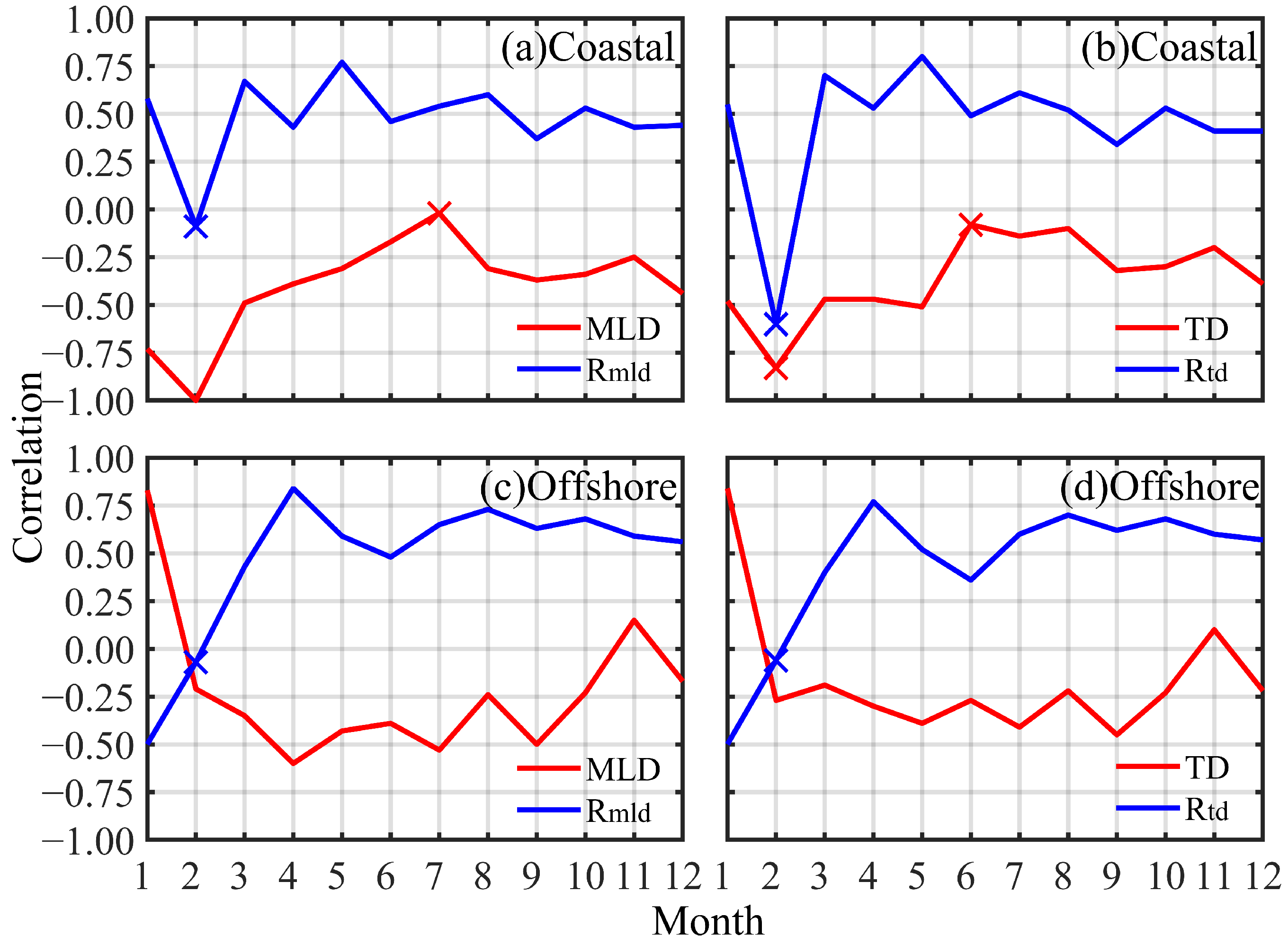
3.2. Effects of the BG on DSST

To further investigate the relationship between DSST and various BG parameters, this study conducts a Spearman correlation analysis between them. Due to the limited amount of data in the first three months, they will be excluded from the overall statistical analysis as well as from the subsequent correlation discussions.

In

Table 2. Monthly Spearman correlation between BG parameters and DSST (C represents coastal regions, O represents offshore regions, and values marked with an asterisk denote correlations that pass the 95% confidence interval; All excludes data from January to March).

Month	T100		SST−T100		MLD		T Thickness		TD		TS
	C	O	C	O	C	O	C	O	C	O	C	O
1	−0.31 *	0.63	0.33	−0.83	−0.73	0.83	−0.50	0.70	−0.48	0.84	0.34 *	−0.83
2	−0.94	0.06 *	0.94	0.16 *	−1.00	−0.21	0.94	−0.34	−0.83 *	−0.27	−0.83 *	0.42
3	−0.35 *	−0.18	0.92	0.18	−0.49	−0.35	−0.88	0.42	−0.47	−0.19	0.92	−0.44
4	−0.38	−0.46	0.42	0.40	−0.39	−0.60	−0.21	0.20	−0.47	−0.30	0.31	−0.14
5	−0.13	−0.19	0.57	0.31	−0.31	−0.43	−0.38	−0.06 *	−0.51	−0.39	0.46	−0.05 *
6	0.35	−0.09 *	0.16	0.43	−0.17	−0.39	0.05 *	0.16	−0.08 *	−0.27	0.11	−0.23
7	0.08	−0.32	0.13	0.48	−0.02 *	−0.53	−0.12	−0.22	−0.14	−0.41	0.11	0.15
8	−0.07	−0.16	0.13	0.23	−0.31	−0.24	0.04 *	−0.18	−0.10	−0.22	−0.08	0.15
9	−0.25	−0.39	0.30	0.47	−0.37	−0.50	−0.18	−0.35	−0.32	−0.45	0.16	0.22
10	−0.18	−0.23	0.27	0.24	−0.34	−0.23	−0.19	−0.19	−0.30	−0.23	0.12	0.03 *
11	−0.08	−0.01 *	0.20	−0.14	−0.25	0.15	−0.08	0.05 *	−0.20	0.10	0.16	−0.26
12	−0.45	−0.31	0.40	0.21	−0.44	−0.17	−0.20	−0.11 *	−0.39	−0.22	0.02 *	0.09 *
All	−0.13	−0.27	0.28	0.37	−0.27	−0.40	−0.11	−0.18	−0.25	−0.35	0.08	0.06

, the monthly correlation represents the Spearman correlation between the time series of BG parameters and DSST, both spatially averaged. T100, MLD, T Thickness, and TD exhibit significant negative correlations with DSST, while SST-T100 and TS exhibit positive correlations. Additionally, offshore correlations generally exceed coastal values during the same months. In terms of correlation coefficients, SST-T100 is more significant than T100. Furthermore, T Thickness and TS generally show lower correlations than the other parameters in each month, with more data failing the significance test. Moreover, the correlations of BG parameters tend to be weaker during the summer months. When T Thickness, TD, and TS exhibit a strong correlation with DSST, SST-T100 exhibits a similar correlation, and vice versa. For example, in May for coastal regions (September for offshore regions), the correlation coefficients of T Thickness, TD, and TS with DSST are −0.38 (−0.35), −0.51 (−0.45), and 0.46 (0.22), respectively, while the correlation for SST-T100 is 0.57 (0.47). Despite the fact that SST-T100, MLD, and TD exhibit the most substantial correlations in the BG parameters, they nevertheless demonstrate relatively weak correlations.

Building on the above analysis, this study further presents statistical scatter plots of DSST against various BG parameters to examine their correspondence and compare their respective regression fits. Figure 5 illustrates these scatter plots, showing the overall Spearman correlation between the time series of each BG parameter and DSST. The results indicate that T100, MLD, TD, and T Thickness exhibit negative correlations with DSST, whereas SST-T100 and TS demonstrate positive correlations. In addition, the ranges of key BG parameters in coastal and offshore regions show notable differences. For instance, T100, SST-T100, and TS are generally wider in coastal regions than in offshore regions, while MLD, TD, and T Thickness exhibit similar distribution ranges across both regions. However, the MLD and TD in offshore regions are concentrated in deeper depth ranges.

To further investigate the relationship between DSST and various BG parameters, this study presents the spatial distribution of the Spearman temporal correlation between BG parameters and DSST, as shown in Figure 6. The results demonstrate that SST-T100 exhibits a stronger correlation with DSST than T100, with a generally positive correlation across the field. In contrast, MLD and TD show a distinct negative correlation throughout most of the field. Additionally, the Spearman correlations of TS and T Thickness with DSST display an intricate spatial pattern with opposite trends, suggesting that a single variable cannot adequately describe the DSST. To better understand the relationship between BG and DSST, it is necessary to conduct a comprehensive analysis incorporating multiple parameters (Figure 6e,f).

The preceding discussion outlined the relationship between DSST and various BG parameters. To further investigate DSST, this study incorporates TC characteristics (R34, Trans, MW) to assess their influence. Therefore, Figure 7 and Figure 8 illustrate the relationships between TC characteristics (R34, Trans, and MW) and BG parameters (MLD and TD) in relation to DSST. In general, TCs with a large radius, slow movement, and strong maximum sustained winds, along with a shallower MLD and TD, are more likely to induce intense DSST.

In coastal regions, when MLD < 40 m, DSST can exceed 1.5 $°\mathrm{C}$ and when TD < 95 m, DSST can easily surpass 1 $°\mathrm{C}$. This suggests that shallow MLD and TD create favorable conditions for stronger DSST. When MLD > 60 m, DSST generally remains below 0.5 $°\mathrm{C}$, regardless of changes in TC characteristics, and when TD > 115 m, DSST rarely exceeds 0.5 $°\mathrm{C}$. This indicates that BG plays a decisive role in limiting DSST. In addition, when R34 > 305 km, DSST can exceed 0.5 $°\mathrm{C}$ regardless of MLD variations.

In offshore regions, when MLD > 90 m or TD > 145 m, DSST generally remains below 0.5 $°\mathrm{C}$ regardless of TC characteristics, signifying that a deep MLD or TD effectively inhibits DSST. When MLD < 70 m or TD < 115 m, DSST can exceed 1 $°\mathrm{C}$, indicating that shallow MLD and TD create a favorable environment for intense DSST. In addition, when R34 > 320 km, DSST can exceed 0.5 $°\mathrm{C}$, largely independent of MLD or TD variations.

It is clear that both TC characteristics and BG are essential. When the MLD or TD is shallow, even unfavorable TC conditions can induce significant DSST, highlighting the important influence of BG in those conditions. Conversely, large R34 and MW and slow Trans can drive a notable DSST regardless of changes in MLD or TD, reflecting the critical role of TC factors. Hence, no single factor uniformly dominates; rather, the interplay between BG and TC ultimately determines the magnitude of DSST.

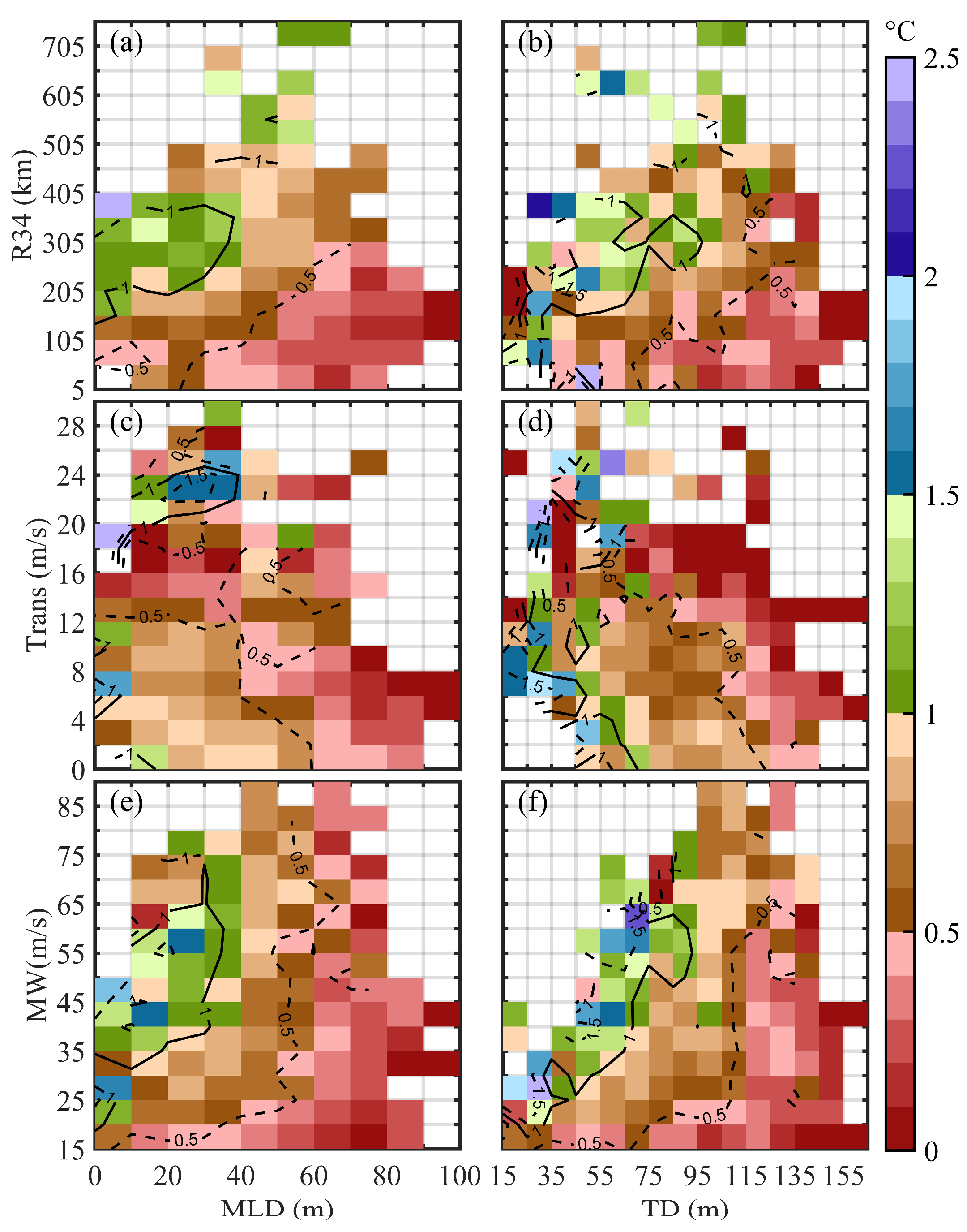
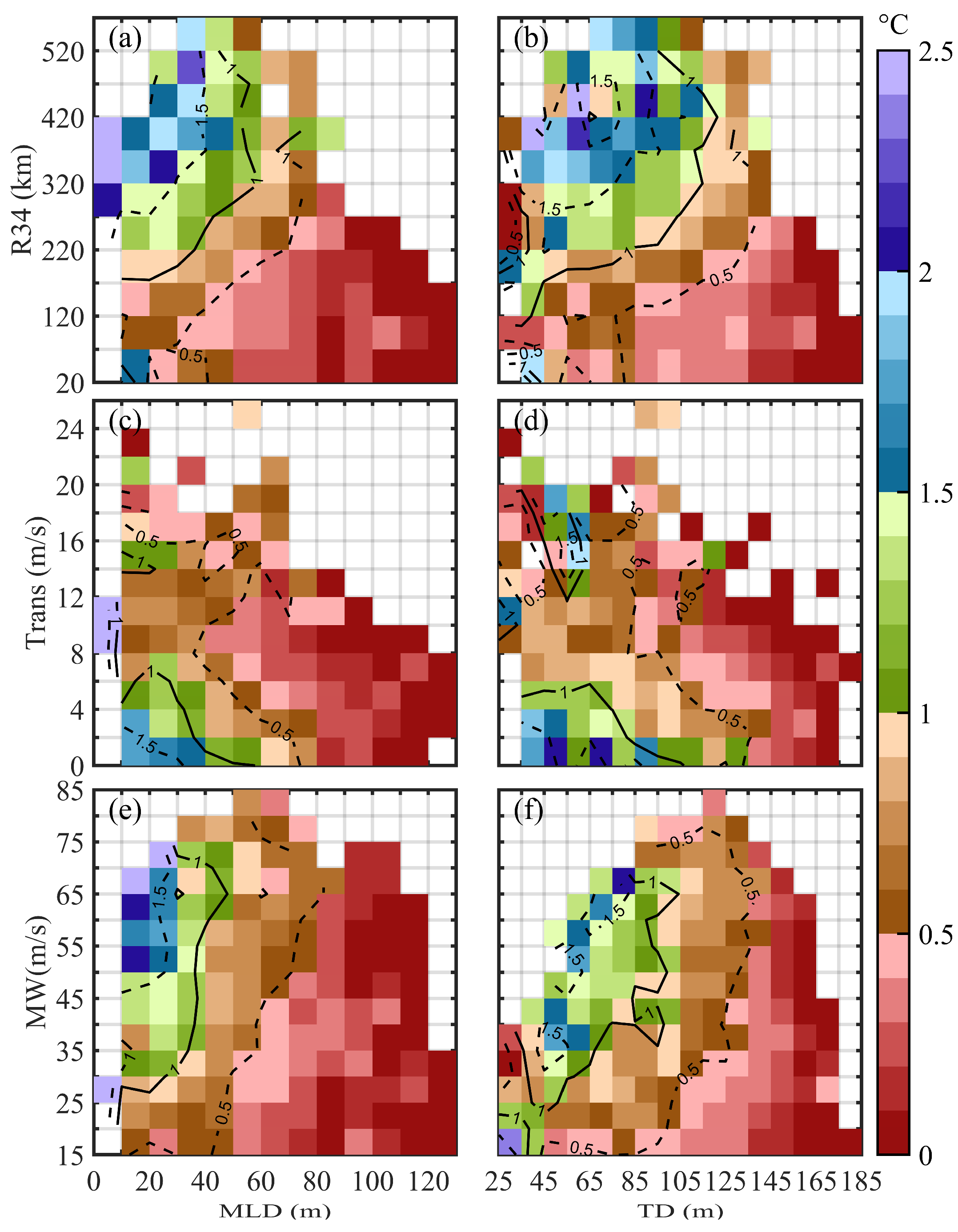
3.3. Synergistic Effects of the BG and TC on DSST

Based on the above analysis, the parameters related to the BG and the characteristics of TC both influence DSST. Larger values of R34 and MW indicate TC characteristics that are favorable for DSST, while larger values of Trans, MLD, and TD reflect TC and BG characteristics that are unfavorable for DSST (Figure 7 and Figure 8). To account for the synergistic effects of TC and BG on DSST, this study introduces the dimensionless parameters ${\mathrm{R}}_{\mathrm{mld}}$ and ${\mathrm{R}}_{\mathrm{td}}$.

First, for the TC, a larger MW indicates stronger energy input from the TC into the ocean, while a larger R34 signifies a broader spatial extent of TC-induced energy input. Additionally, a slower Trans implies a prolonged duration of TC influence which allows the TC’s wind energy input to the same area for a longer time, leading to more pronounced DSST. To comprehensively account for the influence of TC, the TC index (TCI) was formulated,

$$\mathrm{TCI}={\displaystyle \frac{\mathrm{MW}\times {\mathrm{R}}_{34}}{\mathrm{Trans}}}$$

(5)

Next, MLD and TD characterize the influence of the BG on DSST, as they regulate vertical mixing efficiency. Deeper MLD and TD reduce the intensity of DSST, highlighting the constraining effect of the BG on DSST. In contrast, the TCI represents the TC’s capacity to enhance DSST [31]. To capture the synergistic effects of TC and BG on DSST, dimensionless indices ${\mathrm{R}}_{\mathrm{m}\mathrm{l}\mathrm{d}}$ and ${\mathrm{R}}_{\mathrm{t}\mathrm{d}}$ are formulated as follows:

$${\mathrm{R}}_{\mathrm{mld}}={\displaystyle \frac{\mathrm{TCI}}{\mathrm{MLD}}}$$

(6)

$${\mathrm{R}}_{\mathrm{td}}={\displaystyle \frac{\mathrm{TCI}}{\mathrm{TD}}}$$

(7)

The indices ${\mathrm{R}}_{\mathrm{mld}}$ and ${\mathrm{R}}_{\mathrm{td}}$ represent the synergistic effects of the TC and the BG on DSST. These dimensionless metrics quantify the synergistic effects of TC-driven forcing (enhancing cooling through energy input) and oceanic suppression (inhibiting cooling via stratification) in promoting a DSST.

To analyze ${\mathrm{R}}_{\mathrm{mld}}$ and ${\mathrm{R}}_{\mathrm{td}}$, this study presents their climatological spatial distribution and monthly variations, as illustrated in Figure 9 for both coastal and offshore regions. ${\mathrm{R}}_{\mathrm{mld}}$ and ${\mathrm{R}}_{\mathrm{td}}$ exhibit similar spatial and temporal distribution. The climatological spatial distribution reveals that in coastal regions, ${\mathrm{R}}_{\mathrm{mld}}$ and ${\mathrm{R}}_{\mathrm{td}}$ reach their maximum values at 20° N–30° N, gradually decreasing toward both sides of the latitude.

From the climatological monthly temporal distribution of ${\mathrm{R}}_{\mathrm{mld}}$ and ${\mathrm{R}}_{\mathrm{td}}$, it can be observed that in coastal regions, ${\mathrm{R}}_{\mathrm{mld}}$ and ${\mathrm{R}}_{\mathrm{td}}$ reach their maximum values in April, whereas in offshore regions, their peaks occur in August. The peak values of ${\mathrm{R}}_{\mathrm{mld}}$ exceed 10.5 in both regions, while ${\mathrm{R}}_{\mathrm{td}}$ peaks are above 9.5, with ${\mathrm{R}}_{\mathrm{mld}}$ generally larger than ${\mathrm{R}}_{\mathrm{td}}$ during the same period. ${\mathrm{R}}_{\mathrm{mld}}$ and ${\mathrm{R}}_{\mathrm{td}}$ exhibit a similar spatial and temporal distribution to DSST in both coastal and offshore regions. This indicates that the magnitudes of ${\mathrm{R}}_{\mathrm{mld}}$ and ${\mathrm{R}}_{\mathrm{td}}$ can be used to characterize the intensity of DSST. Therefore, ${\mathrm{R}}_{\mathrm{mld}}$ and ${\mathrm{R}}_{\mathrm{td}}$ values exhibit a positive correlation with DSST (Figure 3a, Figure 4a, and Figure 9).

To explore and evaluate the representational capability of the ${\mathrm{R}}_{\mathrm{mld}}$ and ${\mathrm{R}}_{\mathrm{td}}$ for DSST, this study conducts a correlation analysis between ${\mathrm{R}}_{\mathrm{mld}}$ and ${\mathrm{R}}_{\mathrm{td}}$ with DSST.

Table 3. Monthly Spearman correlation analysis between ${\mathrm{R}}_{\mathrm{mld}}$ and R_td with DSST (C represents coastal regions, O represents offshore regions, values marked with an asterisk denote correlations that pass the 95% confidence interval; All excludes data from January to March).

Month	${\mathbf{R}}_{\mathbf{m}\mathbf{l}\mathbf{d}}$		${\mathbf{R}}_{\mathbf{t}\mathbf{d}}$
	C	O	C	O
1	0.58	−0.50	0.55	−0.50
2	−0.09 *	−0.07 *	−0.60 *	−0.06 *
3	0.67	0.43	0.70	0.40
4	0.43	0.84	0.53	0.77
5	0.77	0.59	0.80	0.52
6	0.46	0.48	0.49	0.36
7	0.54	0.65	0.61	0.60
8	0.60	0.73	0.52	0.70
9	0.37	0.63	0.34	0.62
10	0.53	0.68	0.53	0.68
11	0.43	0.59	0.41	0.60
12	0.44	0.56	0.41	0.57
All	0.53	0.66	0.50	0.63

shows the results of the monthly Spearman correlation analysis. From April to December, ${\mathrm{R}}_{\mathrm{mld}}$ and ${\mathrm{R}}_{\mathrm{td}}$ both show a stable positive correlation with DSST, generally showing a more significant correlation in offshore regions compared to coastal regions. In coastal regions, the correlation coefficients of ${\mathrm{R}}_{\mathrm{mld}}$ and ${\mathrm{R}}_{\mathrm{td}}$ peak in May at 0.77 and 0.80, respectively, while in offshore regions, they peak in April at 0.84 and 0.77. Additionally, almost all data pass significance tests. Quantitative comparison in Table 2 reveals that ${\mathrm{R}}_{\mathrm{mld}}$ and ${\mathrm{R}}_{\mathrm{td}}$ exhibit stronger correlations with DSST than MLD and TD, indicating that the incorporation of the TC characteristics alongside the BG parameters provides a more comprehensive description of the DSST.

Although more intense TCs generally lead to larger DSST, the increased correlations between ${\mathrm{R}}_{\mathrm{mld}}$ and DSST, as well as ${\mathrm{R}}_{\mathrm{td}}$ and DSST, indicate that these indices offer a more effective representation of the complex interplay between TC and BG. Specifically, they help capture cases where relatively weak TCs—when occurring under favorable oceanic backgrounds—can induce greater surface cooling than stronger TCs under less favorable conditions. By integrating both TC and BG into unified indices, ${\mathrm{R}}_{\mathrm{mld}}$ and ${\mathrm{R}}_{\mathrm{td}}$ provide a more comprehensive and physically grounded framework for analyzing DSST responses.

Building on the above analysis, Figure 10 presents scatter plots of DSST against ${\mathrm{R}}_{\mathrm{mld}}$ and ${\mathrm{R}}_{\mathrm{td}}$, showing their overall Spearman correlation and demonstrating that both metrics generally exhibit a more pronounced positive correlation with DSST. The values of the ${\mathrm{R}}_{\mathrm{mld}}$ are concentrated between seven and thirteen, while ${\mathrm{R}}_{\mathrm{td}}$ values range from six to twelve, with a similar distribution in both coastal and offshore regions. The correlation coefficients of the MLD and TD with DSST are −0.27 (−0.40) and −0.25 (−0.35) for coastal (offshore) regions, respectively. When further considering the TC characteristics, the correlation coefficients of ${\mathrm{R}}_{\mathrm{mld}}$ and ${\mathrm{R}}_{\mathrm{td}}$ with DSST increase to 0.53 (0.66) and 0.50 (0.63).

To further investigate the relationship between DSST and these two dimensionless metrics, this study also presents the spatial distribution of their Spearman temporal correlation coefficients with DSST, as shown in Figure 11. Both ${\mathrm{R}}_{\mathrm{m}\mathrm{l}\mathrm{d}}$ and ${\mathrm{R}}_{\mathrm{t}\mathrm{d}}$ exhibit more consistent and significant correlations with DSST than MLD and TD, and show a broader spatial extent that passes the significance test (Figure 6 and Figure 11).

${\mathrm{R}}_{\mathrm{m}\mathrm{l}\mathrm{d}}$ and ${\mathrm{R}}_{\mathrm{t}\mathrm{d}}$ comprehensively consider the maximum sustained wind speed, the translation speed, the 34-kt wind radius of the TC, and the BG conditions. Consequently, in describing DSST, ${\mathrm{R}}_{\mathrm{m}\mathrm{l}\mathrm{d}}$ and ${\mathrm{R}}_{\mathrm{t}\mathrm{d}}$ provide more stable and robust representation compared to solely using BG parameters.

4. Discussion

DSST is defined as the SST difference between 1–5 days before and after the passage of each TC. This time window is supported by previous studies showing that SST typically recovers to its climatological state within 5 days, and that the most significant cooling occurs during this period [8]. A spatial domain of 6° × 6° centered on the TC location is used, which encompasses the typical wind radius (~300 km) where SST responses are most pronounced. Jin et al. [66] have shown that while the magnitude of DSST may vary with different temporal and spatial scales, the overall seasonal and spatial patterns remain consistent, supporting the robustness of this approach.

Da et al. [24] analyzed TC parameters (Vmax, Vtrans, and R34) and BG parameters (Grad-T, Grad-S, and MLD) across individual ocean basins. The spatial distributions of the MLD and DSST, as well as their correlations in the WNP, are similar to those presented in this study (Figure 4 and Figure 6). Beyond MLD, our findings demonstrate that the correlation between SST-T100 and DSST was also higher than that of T100 (Table 2), which is consistent with Vincent et al. [56], who pointed out that SST-T100 actually improved the ability to predict TC. In addition, this study primarily investigates the correlations between BG parameters (T100, SST-T100, MLD, TD, T Thickness, and TS) and DSST (Figure 5). In contrast, Pun et al. [35] focused on the correlations of R34, Vmax, translation speed (Uh), and upper ocean heat content (UOHC) with DSST, presenting values of 0.49, 0.46, −0.38, and −0.37, respectively. Consequently, whether considering BG or TC parameters individually, their correlations with DSST rarely exceed 0.5. However, when BG and TC parameters are combined, as demonstrated in this study, the correlation increases (Figure 11). Furthermore, compared to MLD and TD, the ${\mathrm{R}}_{\mathrm{mld}}$ and ${\mathrm{R}}_{\mathrm{td}}$ exhibit more stable correlations with DSST across both spatial and temporal scales (Figure 12).

Our results show that coastal regions correlation between ${\mathrm{R}}_{\mathrm{m}\mathrm{l}\mathrm{d}}$ and ${\mathrm{R}}_{\mathrm{t}\mathrm{d}}$ with DSST exceed 0.75 in May, maintaining values around 0.5 in other months with small seasonal variation (Table 3, Figure 12). In offshore regions, the maximum correlation reaches above 0.75 in April, remaining near 0.5 during most other months. In contrast, Spearman correlations involving MLD and TD exhibit substantial monthly variability in both coastal and offshore regions, even switching between positive and negative values. These findings indicate that ${\mathrm{R}}_{\mathrm{m}\mathrm{l}\mathrm{d}}$ and ${\mathrm{R}}_{\mathrm{t}\mathrm{d}}$ to some extent enhance correlations with DSST.

In this study, we construct dimensionless parameters ${\mathrm{R}}_{\mathrm{m}\mathrm{l}\mathrm{d}}$ and ${\mathrm{R}}_{\mathrm{t}\mathrm{d}}$ to characterize DSST. In addition, there are also many other excellent approaches to describe it. Oey [57] proposed a dimensionless (nonlinear) function $\mathsf{\Psi }$ representing DSST, determined by both TC parameters and upper-layer BG characteristics, and the explained variance in their results is ${\mathrm{r}}^2\approx 0.6$. Cui et al. [36] built a model using an efficient and robust machine learning-based method with 12 predictors related to TC characteristics and pre-storm ocean states. Their findings indicate that TC intensity, translation speed, size, pre-storm MLD, and SST are the dominant factors in determining the magnitude of the SST response. Moreover, Vincent et al. [12] introduced the Wind Power Index (WPi) and Cooling Inhibition Index (CI). WPi primarily considered DSST impacts from TC parameters such as MW, translation speed, and size, while CI explained the pre-TC upper-ocean stratification resistance to DSST. Therefore, WPi and CI describe DSST variability from TC and BG perspectives. The ${\mathrm{R}}_{\mathrm{mld}}$ and ${\mathrm{R}}_{\mathrm{td}}$ proposed in this study systematically incorporates the synergistic effects of BG and TC, achieving a more comprehensive analysis of DSST.

5. Conclusions

Based on the satellite observation data and reanalysis data, this study analyzes the distribution characteristics of the DSST under TC conditions in the WNP as well as the impacts of the TC characteristics and BG structure on the DSST. Further, combining the TC and BG parameters, this study proposes the dimensionless metrics ${\mathrm{R}}_{\mathrm{mld}}$ and ${\mathrm{R}}_{\mathrm{td}}$ to better characterize the spatial and temporal distribution of the DSST.

In the WNP, the magnitude of DSST exhibits significant temporal and spatial variation. The majority of the TC occurrences are concentrated from July to October in both coastal and offshore regions, with the DSST amplitude exceeding 0.6 $°\mathrm{C}$. DSST reaches its maximum in September for coastal regions and in August for offshore regions, with both exceeding 0.85 $°\mathrm{C}$ (Figure 2b and Figure 3a).

In terms of the BG parameters, MLD and TD are effective in representing DSST. The correlations of MLD and TD with DSST in offshore regions are −0.40 and −0.35, respectively, which is more significant than the correlations of −0.27 and −0.25 in coastal regions (Figure 5c,d). However, it is insufficient to only consider BG factors; therefore, we also take the impact of TCs into account. In coastal regions, when MLD > 60 m, DSST generally remains below 0.5 $°\mathrm{C}$, regardless of changes in TC characteristics, and when TD > 115 m, DSST rarely exceeds 1 $°\mathrm{C}$. In addition, when R34 > 305 km, DSST can exceed 0.5 $°\mathrm{C}$ regardless of MLD variations. In offshore regions, when MLD > 90 m or TD > 145 m, DSST generally remains below 0.5 $°\mathrm{C}$ regardless of TC characteristics. In addition, when R34 > 320 km, DSST can exceed 0.5 $°\mathrm{C}$, largely independent of MLD or TD variations. It is clear that the interplay between BG and TC ultimately determines the magnitude of DSST. Based on the above analysis, larger values of R34 and MW are favorable for DSST, while larger values of Trans, MLD, and TD are unfavorable for DSST (Figure 7 and Figure 8). To account for the synergistic effects of TC and BG on DSST, this study introduces the dimensionless parameters ${\mathrm{R}}_{\mathrm{mld}}$ and ${\mathrm{R}}_{\mathrm{td}}$.

In both temporal and spatial dimensions, ${\mathrm{R}}_{\mathrm{mld}}$ and ${\mathrm{R}}_{\mathrm{td}}$ can better characterize DSST than MLD and TD. The Spearman correlations of ${\mathrm{R}}_{\mathrm{m}\mathrm{l}\mathrm{d}}$ and ${\mathrm{R}}_{\mathrm{t}\mathrm{d}}$ with coastal DSST can reach 0.53 and 0.50, respectively, while in offshore regions, the correlations are up to 0.66 and 0.63. Moreover, the correlations exhibit greater spatial consistency and better pass the test of significance (Figure 5, Figure 6, Figure 10, Figure 11 and Figure 12). Since ${\mathrm{R}}_{\mathrm{mld}}$ and ${\mathrm{R}}_{\mathrm{td}}$ incorporate TC parameters such as MW, Trans, R34, and the BG conditions, the ${\mathrm{R}}_{\mathrm{m}\mathrm{l}\mathrm{d}}$ and ${\mathrm{R}}_{\mathrm{t}\mathrm{d}}$ are more stable across different seasons, making them more representative than the solely BG parameters. Indeed, more intense TCs tend to produce a larger DSST, which is consistent with existing literature. However, the novel contribution of this study lies in its comprehensive approach. The key innovation here is not just the expected correlation between TC or BG and DSST, but the ability to capture cases where relatively weak TCs—when occurring under favorable oceanic backgrounds—can induce greater surface cooling than stronger TCs under less favorable conditions. This insight improves our understanding of the complex interaction between TCs and BG, enabling better forecasting of DSST and related phenomena in different TC scenarios.

This study specifically focuses on the oceanic conditions prior to the arrival of TCs. Incorporating parameters such as ${\mathrm{R}}_{\mathrm{mld}}$ and ${\mathrm{R}}_{\mathrm{td}}$ captures the synergistic effects of BG and TC on DSST. This approach enables us to estimate and provide early warnings for areas that will soon be affected by the TCs. Specifically, by predicting the changes in DSST before the TC reaches the coast, we improve our ability to forecast TC intensity and anticipate potential impacts, which is critical for disaster preparedness and mitigation in coastal regions. But in constructing the indices, only the more significant temporal and spatial correlations of MLD and TD are considered, and the more complex TS and T Thickness are not considered. Future studies should systematically explore the synergistic effects of various BG and TC parameters on the DSST. Moreover, while investigating the ocean’s response to TCs, it is also crucial to analyze the ocean’s impact on the TCs.

References

1. Emanuel, K. Tropical Cyclones. Annu. Rev. Earth Planet. Sci. 2003, 31, 75–104. [Google Scholar] [CrossRef]
2. Li, A.; Guan, S.; Mo, D.; Hou, Y.; Hong, X.; Liu, Z. Modeling Wave Effects on Storm Surge from Different Typhoon Intensities and Sizes in the South China Sea. Estuar. Coast. Shelf Sci. 2020, 235, 106551. [Google Scholar] [CrossRef]
3. Emanuel, K.A. Thermodynamic Control of Hurricane Intensity. Nature 1999, 401, 665–669. [Google Scholar] [CrossRef]
4. Jin, F.-F.; Boucharel, J.; Lin, I.-I. Eastern Pacific Tropical Cyclones Intensified by El Niño Delivery of Subsurface Ocean Heat. Nature 2014, 516, 82–85. [Google Scholar] [CrossRef]
5. Lin, I.-I.; Black, P.; Price, J.F.; Yang, C.-Y.; Chen, S.S.; Lien, C.-C.; Harr, P.; Chi, N.-H.; Wu, C.-C.; D’Asaro, E.A. An Ocean Coupling Potential Intensity Index for Tropical Cyclones. Geophys. Res. Lett. 2013, 40, 1878–1882. [Google Scholar] [CrossRef]
6. Mei, W.; Xie, S.-P.; Primeau, F.; McWilliams, J.C.; Pasquero, C. Northwestern Pacific Typhoon Intensity Controlled by Changes in Ocean Temperatures. Sci. Adv. 2015, 1, e1500014. [Google Scholar] [CrossRef] [PubMed]
7. Bracken, W.E.; Bosart, L.F. The Role of Synoptic-Scale Flow during Tropical Cyclogenesis over the North Atlantic Ocean. Mon. Weather. Rev. 2000, 128, 353–376. [Google Scholar] [CrossRef]
8. Dare, R.A.; McBride, J.L. Sea Surface Temperature Response to Tropical Cyclones. Mon. Weather Rev. 2011, 139, 3798–3808. [Google Scholar] [CrossRef]
9. Gray, W. Global View of the Origin of Tropical Disturbances and Storms. Mon. Weather Rev. 1968, 96, 669–700. [Google Scholar] [CrossRef]
10. Cione, J.J.; Uhlhorn, E.W. Sea Surface Temperature Variability in Hurricanes: Implications with Respect to Intensity Change. Mon. Weather Rev. 2003, 131, 1783–1796. [Google Scholar] [CrossRef]
11. Price, J.F. Upper Ocean Response to a Hurricane. J. Phys. Oceanogr. 1981, 11, 153–175. [Google Scholar] [CrossRef]
12. Vincent, E.M.; Lengaigne, M.; Madec, G.; Vialard, J.; Samson, G.; Jourdain, N.C.; Menkes, C.E.; Jullien, S. Processes Setting the Characteristics of Sea Surface Cooling Induced by Tropical Cyclones. J. Geophys. Res. Oceans 2012, 117, C02020. [Google Scholar] [CrossRef]
13. Lin, I.-I.; Pun, I.-F.; Wu, C.-C. Upper-Ocean Thermal Structure and the Western North Pacific Category 5 Typhoons. Part II: Dependence on Translation Speed. Mon. Weather Rev. 2009, 137, 3744–3757. [Google Scholar] [CrossRef]
14. Shay, L.K.; Brewster, J.K. Oceanic Heat Content Variability in the Eastern Pacific Ocean for Hurricane Intensity Forecasting. Mon. Weather Rev. 2010, 138, 2110–2131. [Google Scholar] [CrossRef]
15. Glenn, S.M.; Miles, T.N.; Seroka, G.N.; Xu, Y.; Forney, R.K.; Yu, F.; Roarty, H.; Schofield, O.; Kohut, J. Stratified Coastal Ocean Interactions with Tropical Cyclones. Nat. Commun. 2016, 7, 10887. [Google Scholar] [CrossRef]
16. Guan, S.; Zhao, W.; Sun, L.; Zhou, C.; Liu, Z.; Hong, X.; Zhang, Y.; Tian, J.; Hou, Y. Tropical Cyclone-Induced Sea Surface Cooling over the Yellow Sea and Bohai Sea in the 2019 Pacific Typhoon Season. J. Mar. Syst. 2021, 217, 103509. [Google Scholar] [CrossRef]
17. Mahapatra, D.K.; Rao, A.D.; Babu, S.V.; Srinivas, C. Influence of Coast Line on Upper Ocean’s Response to the Tropical Cyclone. Geophys. Res. Lett. 2007, 34, L17603. [Google Scholar] [CrossRef]
18. Shen, W.; Ginis, I. Effects of Surface Heat Flux-Induced Sea Surface Temperature Changes on Tropical Cyclone Intensity. Geophys. Res. Lett. 2003, 30, 1933. [Google Scholar] [CrossRef]
19. Greatbatch, R.J. On the Response of the Ocean to a Moving Storm: Parameters and Scales. J. Phys. Oceanogr. 1984, 14, 59–78. [Google Scholar] [CrossRef]
20. Jacob, S.D.; Shay, L.K.; Mariano, A.J.; Black, P.G. The 3D Oceanic Mixed Layer Response to Hurricane Gilbert. J. Phys. Oceanogr. 2000, 30, 1407–1429. [Google Scholar] [CrossRef]
21. Lin, S.; Zhang, W.-Z.; Shang, S.-P.; Hong, H.-S. Ocean Response to Typhoons in the Western North Pacific: Composite Results from Argo Data. Deep Sea Res. Part Oceanogr. Res. Pap. 2017, 123, 62–74. [Google Scholar] [CrossRef]
22. Peng, Y.; Tian, D.; Zhou, F.; Zhang, H.; Ma, X.; Zeng, D.; Meng, Q.; Zhou, B.; Ye, R.; Chen, Y.; et al. Observed Oceanic Response to Tropical Cyclone Amphan (2020) from a Subsurface Mooring in the Bay of Bengal. Prog. Oceanogr. 2023, 219, 103148. [Google Scholar] [CrossRef]
23. Shay, L.K.; Black, P.G.; Mariano, A.J.; Hawkins, J.D.; Elsberry, R.L. Upper Ocean Response to Hurricane Gilbert. J. Geophys. Res. Oceans 1992, 97, 20227–20248. [Google Scholar] [CrossRef]
24. Da, N.D.; Foltz, G.R.; Balaguru, K.; Fernald, E. Stronger Tropical Cyclone–Induced Ocean Cooling in Near-Coastal Regions Compared to the Open Ocean. J. Clim. 2023, 36, 6447–6463. [Google Scholar] [CrossRef]
25. Zheng, Y.; Ma, Z.; Tang, J.; Zhang, Z. The Coastal Effect on Ahead-of-Eye-Center Cooling Induced by Tropical Cyclones. J. Phys. Oceanogr. 2023, 53, 1519–1534. [Google Scholar] [CrossRef]
26. Chiang, T.-L.; Wu, C.-R.; Oey, L.-Y. Typhoon Kai-Tak: An Ocean’s Perfect Storm. J. Phys. Oceanogr. 2011, 41, 221–233. [Google Scholar] [CrossRef]
27. Guan, S.; Zhao, W.; Huthnance, J.; Tian, J.; Wang, J. Observed Upper Ocean Response to Typhoon Megi (2010) in the Northern South China Sea. J. Geophys. Res. Oceans 2014, 119, 3134–3157. [Google Scholar] [CrossRef]
28. Ren, D.; Han, S.; Wang, S. Upper Ocean Responses to Tropical Cyclone Mekunu (2018) in the Arabian Sea. J. Mar. Sci. Eng. 2024, 12, 1177. [Google Scholar] [CrossRef]
29. Bender, M.A.; Ginis, I.; Kurihara, Y. Numerical Simulations of Tropical Cyclone-Ocean Interaction with a High-Resolution Coupled Model. J. Geophys. Res. Atmos. 1993, 98, 23245–23263. [Google Scholar] [CrossRef]
30. Lin, I.-I.; Wu, C.-C.; Emanuel, K.A.; Lee, I.-H.; Wu, C.-R.; Pun, I.-F. The Interaction of Supertyphoon Maemi (2003) with a Warm Ocean Eddy. Mon. Weather Rev. 2005, 133, 2635. [Google Scholar] [CrossRef]
31. Price, J.F. Internal Wave Wake of a Moving Storm. Part I. Scales, Energy Budget and Observations. J. Phys. Oceanogr. 1983, 13, 949–965. [Google Scholar] [CrossRef]
32. Pun, I.-F.; Lin, I.-I.; Lien, C.-C.; Wu, C.-C. Influence of the Size of Supertyphoon Megi (2010) on SST Cooling. Mon. Weather Rev. 2018, 146, 661–677. [Google Scholar] [CrossRef]
33. Pun, I.-F.; Chan, J.C.L.; Lin, I.-I.; Chan, K.T.F.; Price, J.F.; Ko, D.S.; Lien, C.-C.; Wu, Y.-L.; Huang, H.-C. Rapid Intensification of Typhoon Hato (2017) over Shallow Water. Sustainability 2019, 11, 3709. [Google Scholar] [CrossRef]
34. Wang, H.; Li, J.; Song, J.; Leng, H.; Wang, H.; Zhang, Z.; Zhang, H.; Zheng, M.; Yang, X.; Wang, C. The Abnormal Track of Super Typhoon Hinnamnor (2022) and Its Interaction with the Upper Ocean. Deep. Sea Res. Part Oceanogr. Res. Pap. 2023, 201, 104160. [Google Scholar] [CrossRef]
35. Pun, I.-F.; Knaff, J.A.; Sampson, C.R. Uncertainty of Tropical Cyclone Wind Radii on Sea Surface Temperature Cooling. J. Geophys. Res. Atmos. 2021, 126, e2021JD034857. [Google Scholar] [CrossRef]
36. Cui, H.; Tang, D.; Mei, W.; Liu, H.; Sui, Y.; Gu, X. Predicting Tropical Cyclone-Induced Sea Surface Temperature Responses Using Machine Learning. Geophys. Res. Lett. 2023, 50, e2023GL104171. [Google Scholar] [CrossRef]
37. Moon, I.-J.; Kwon, S.J. Impact of Upper-Ocean Thermal Structure on the Intensity of Korean Peninsular Landfall Typhoons. Prog. Oceanogr. 2012, 105, 61–66. [Google Scholar] [CrossRef]
38. Balaguru, K.; Foltz, G.R.; Leung, L.R.; Hagos, S.M. Impact of Rainfall on Tropical Cyclone-Induced Sea Surface Cooling. Geophys. Res. Lett. 2022, 49, e2022GL098187. [Google Scholar] [CrossRef]
39. D’Asaro, E.A.; Black, P.G.; Centurioni, L.R.; Chang, Y.-T.; Chen, S.S.; Foster, R.C.; Graber, H.C.; Harr, P.; Hormann, V.; Lien, R.-C.; et al. Impact of Typhoons on the Ocean in the Pacific. Bull. Am. Meteorol. Soc. 2014, 95, 1405–1418. [Google Scholar] [CrossRef]
40. Knaff, J.A.; DeMaria, M.; Sampson, C.R.; Peak, J.E.; Cummings, J.; Schubert, W.H. Upper Oceanic Energy Response to Tropical Cyclone Passage. J. Clim. 2013, 26, 2631–2650. [Google Scholar] [CrossRef]
41. Lin, I.-I.; Rogers, R.F.; Huang, H.-C.; Liao, Y.-C.; Herndon, D.; Yu, J.-Y.; Chang, Y.-T.; Zhang, J.A.; Patricola, C.M.; Pun, I.-F.; et al. A Tale of Two Rapidly Intensifying Supertyphoons: Hagibis (2019) and Haiyan (2013). Bull. Am. Meteorol. Soc. 2021, 102, E1645–E1664. [Google Scholar] [CrossRef]
42. Mei, W.; Lien, C.-C.; Lin, I.-I.; Xie, S.-P. Tropical Cyclone–Induced Ocean Response: A Comparative Study of the South China Sea and Tropical Northwest Pacific. J. Clim. 2015, 28, 5952–5968. [Google Scholar] [CrossRef]
43. Potter, H.; DiMarco, S.F.; Knap, A.H. Tropical Cyclone Heat Potential and the Rapid Intensification of Hurricane Harvey in the Texas Bight. J. Geophys. Res. Oceans 2019, 124, 2440–2451. [Google Scholar] [CrossRef]
44. Zhuang, Z.; Yang, Y.; Shu, Q.; Song, Z.; Zhao, B.; Yuan, Y. Variability of Non-Breaking Surface-Wave Induced Mixing and Its Effects on Ocean Thermodynamical Structure in the Northwest Pacific during Typhoon Lekima (2019). Deep. Sea Res. Part Oceanogr. Res. Pap. 2023, 202, 104178. [Google Scholar] [CrossRef]
45. Chan, J.C.L.; Duan, Y.; Shay, L.K. Tropical Cyclone Intensity Change from a Simple Ocean–Atmosphere Coupled Model. J. Atmos. Sci. 2001, 58, 154–172. [Google Scholar] [CrossRef]
46. Maneesha, K.; Murty, V.S.N.; Ravichandran, M.; Lee, T.; Yu, W.; McPhaden, M.J. Upper Ocean Variability in the Bay of Bengal during the Tropical Cyclones Nargis and Laila. Prog. Oceanogr. 2012, 106, 49–61. [Google Scholar] [CrossRef]
47. Mei, W.; Pasquero, C. Restratification of the Upper Ocean after the Passage of a Tropical Cyclone: A Numerical Study. J. Phys. Oceanogr. 2012, 42, 1377–1401. [Google Scholar] [CrossRef]
48. Wang, G.; Wu, L.; Johnson, N.C.; Ling, Z. Observed Three-Dimensional Structure of Ocean Cooling Induced by Pacific Tropical Cyclones. Geophys. Res. Lett. 2016, 43, 7632–7638. [Google Scholar] [CrossRef]
49. Wu, C.-R.; Chang, Y.-L.; Oey, L.-Y.; Chang, C.-W.J.; Hsin, Y.-C. Air-Sea Interaction between Tropical Cyclone Nari and Kuroshio. Geophys. Res. Lett. 2008, 35, L12605. [Google Scholar] [CrossRef]
50. Yu, J.; Zhang, H.; Wang, H.; Tian, D.; Li, J. Upper-Ocean Structure Variability in the Northwest Pacific Ocean in Response to Tropical Cyclones. Front. Mar. Sci. 2023, 10, 1245348. [Google Scholar] [CrossRef]
51. Balaguru, K.; Chang, P.; Saravanan, R.; Leung, L.R.; Xu, Z.; Li, M.; Hsieh, J.-S. Ocean Barrier Layers’ Effect on Tropical Cyclone Intensification. Proc. Natl. Acad. Sci. USA 2012, 109, 14343–14347. [Google Scholar] [CrossRef] [PubMed]
52. Balaguru, K.; Foltz, G.R.; Leung, L.R.; Asaro, E.D.; Emanuel, K.A.; Liu, H.; Zedler, S.E. Dynamic Potential Intensity: An Improved Representation of the Ocean’s Impact on Tropical Cyclones. Geophys. Res. Lett. 2015, 42, 6739–6746. [Google Scholar] [CrossRef]
53. Balaguru, K.; Foltz, G.R.; Leung, L.-Y.; Kaplan, J.; Xu, W.; Reul, N.; Chapron, B. Pronounced Impact of Salinity on Rapidly Intensifying Tropical Cyclones. Bull. Am. Meteorol. Soc. 2020, 101, E1497–E1511. [Google Scholar] [CrossRef]
54. Miles, T.N.; Coakley, S.J.; Engdahl, J.M.; Rudzin, J.E.; Tsei, S.; Glenn, S.M. Ocean Mixing during Hurricane Ida (2021): The Impact of a Freshwater Barrier Layer. Front. Mar. Sci. 2023, 10, 1224609. [Google Scholar] [CrossRef]
55. Neetu, S.; Lengaigne, M.; Vincent, E.M.; Vialard, J.; Madec, G.; Samson, G.; Ramesh Kumar, M.R.; Durand, F. Influence of Upper-Ocean Stratification on Tropical Cyclone-Induced Surface Cooling in the Bay of Bengal. J. Geophys. Res. Oceans 2012, 117, C12020. [Google Scholar] [CrossRef]
56. Vincent, E.M.; Lengaigne, M.; Vialard, J.; Madec, G.; Jourdain, N.C.; Masson, S. Assessing the Oceanic Control on the Amplitude of Sea Surface Cooling Induced by Tropical Cyclones. J. Geophys. Res. Oceans 2012, 117, C05023. [Google Scholar] [CrossRef]
57. Oey, L. A Simple Model of Sea-Surface Cooling under a Tropical Cyclone. J. Mar. Sci. Eng. 2023, 11, 397. [Google Scholar] [CrossRef]
58. Doong, D.-J.; Peng, J.-P.; Babanin, A.V. Field Investigations of Coastal Sea Surface Temperature Drop after Typhoon Passages. Earth Syst. Sci. Data 2019, 11, 323–340. [Google Scholar] [CrossRef]
59. Knapp, K.R.; Kruk, M.C.; Levinson, D.H.; Diamond, H.J.; Neumann, C.J. The International Best Track Archive for Climate Stewardship (IBTrACS): Unifying Tropical Cyclone Data. Bull. Am. Meteorol. Soc. 2010, 91, 363–376. [Google Scholar] [CrossRef]
60. Da, N.D.; Foltz, G.R.; Balaguru, K. A Satellite-Derived Upper-Ocean Stratification Data Set for the Tropical North Atlantic with Potential Applications for Hurricane Intensity Prediction. J. Geophys. Res. Oceans 2020, 125, e2019JC015980. [Google Scholar] [CrossRef]
61. Jean-Michel, L.; Eric, G.; Romain, B.-B.; Gilles, G.; Angélique, M.; Marie, D.; Clément, B.; Mathieu, H.; Olivier, L.G.; Charly, R.; et al. The Copernicus Global 1/12° Oceanic and Sea Ice GLORYS12 Reanalysis. Front. Earth Sci. 2021, 9, 698876. [Google Scholar] [CrossRef]
62. He, Y.; Lin, X.; Han, G.; Liu, Y.; Zhang, H. The Different Dynamic Influences of Typhoon Kalmaegi on Two Pre-Existing Anticyclonic Ocean Eddies. Ocean Sci. 2024, 20, 621–637. [Google Scholar] [CrossRef]
63. Yu, J.; Lv, H.; Tan, S.; Wang, Y. Tropical Cyclone-Induced Sea Surface Temperature Responses in the Northern Indian Ocean. J. Mar. Sci. Eng. 2023, 11, 2196. [Google Scholar] [CrossRef]
64. Kara, A.B.; Rochford, P.A.; Hurlburt, H.E. An Optimal Definition for Ocean Mixed Layer Depth. J. Geophys. Res. Oceans 2000, 105, 16803–16821. [Google Scholar] [CrossRef]
65. Fiedler, P.C. Comparison of Objective Descriptions of the Thermocline. Limnol. Oceanogr. Methods 2010, 8, 313–325. [Google Scholar] [CrossRef]
66. Jin, M.; Zhao, Z.; Wu, R.; Zhu, P. Latitudinal and Seasonal Variations in Tropical Cyclone-Induced Ocean Surface Cooling in the Tropical Western North Pacific. J. Meteorol. Res. 2023, 37, 790–801. [Google Scholar] [CrossRef]
Figure 1. Flowchart of the study.
Jmse 13 00955 g001
Figure 2. Spatial and temporal distribution of 3-h TC observations in the WNP. (a) Spatial distribution of TC observations (2002–2020), calculated on a 1 ° × 1 ° grid; (b) Monthly distribution of TC observations among coastal (blue) and offshore (red) regions. The black dashed line indicates the 500 km boundary.
Jmse 13 00955 g002
Figure 3. Climatological monthly variations of BG parameters in the WNP. (a) DSST; (b) T100; (c) SST-T100; (d) MLD; (e) TS; (f) T Thickness; (g) TD.
Jmse 13 00955 g003
Figure 4. The climatological spatial distribution of the DSST and BG parameters: (a) DSST; (b) T100; (c) SST-T100; (d) MLD; (e) TD; (f) T Thickness; and (g) TS. The black dashed line indicates the 500 km boundary.
Jmse 13 00955 g004
Figure 5. Correlation of the DSST with (a) T100; (b) SST-T100; (c) MLD; (d) TD; (e) T Thickness; and (f) TS. The lines in the figure represent the regression fits ( R C represents coastal regions, blue; R O represents offshore regions, yellow).
Jmse 13 00955 g005
Figure 6. Spatial distribution of the Spearman temporal correlation between BG parameters and DSST. (a) T100; (b) SST-T100; (c) MLD; (d) TD; (e) T Thickness; (f) TS. Black dots represent regions passing the 95% confidence level. The black dashed line indicates the 500 km boundary.
Jmse 13 00955 g006
Figure 7. Relationship between coastal DSST and MLD (left panel) or TD (right panel) under different conditions of (a,b) R34, (c,d) Trans and (e,f) MW. The black solid and dashed lines are contour lines.
Jmse 13 00955 g007
Figure 8. Relationship between offshore DSST and MLD (left panel) or TD (right panel) under different conditions of (a,b) R34, (c,d) Trans, and (e,f) MW. The black solid and dashed lines are contour lines.
Jmse 13 00955 g008
Figure 9. Climatological spatial and temporal distribution of (a,c) R mld and (b,d) R td . Values are shown as lg. The black dashed line indicates the 500 km boundary.
Jmse 13 00955 g009
Figure 10. Same as Figure 5 but for (a) R m l d and (b) R t d ( R C represents coastal regions, blue; R O represents offshore regions, yellow).
Jmse 13 00955 g010
Figure 11. Same as Figure 6. But for (a) R mld and (b) R td . The black dashed line indicates the 500 km boundary.
Jmse 13 00955 g011
Figure 12. Comparative analysis of the correlation between the BG parameters (red line) and the metrics ( R mld and R td , blue line) with DSST. (The symbol × denotes a failure to achieve the 95% significance level). The upper panel shows coastal regions and the lower panel shows offshore regions.
Jmse 13 00955 g012