Article

Scenario-Based Economic Analysis of Underwater Biofouling Using Artificial Intelligence

1
Division of Marine Engineering, National Korea Maritime and Ocean University, Busan 49112, Republic of Korea
2
Interdisciplinary Major of Maritime and AI Convergence, National Korea Maritime and Ocean University, Busan 49112, Republic of Korea
3
Division of Marine System Engineering, National Korea Maritime and Ocean University, Busan 49112, Republic of Korea
4
Division of Navigation Convergence Studies, National Korea Maritime and Ocean University, Busan 49112, Republic of Korea
*
Authors to whom correspondence should be addressed.
J. Mar. Sci. Eng. 2025, 13(5), 952; https://doi.org/10.3390/jmse13050952
Submission received: 17 April 2025 / Revised: 7 May 2025 / Accepted: 12 May 2025 / Published: 14 May 2025
(This article belongs to the Section Ocean Engineering)

Abstract

:
This study presents a novel framework to evaluate the impact of a certain cycle of underwater hull and propeller cleaning. The artificial neural network model was created to predict fuel consumption, and the coefficients for the six voyages were calculated. Three scenarios, in which the coefficients changed in different ways, were established, and the monthly fuel consumption values were calculated accordingly. The annual fuel cost saving when the cycle of underwater hull and propeller cleaning was four months was USD 10,402–26,685, and it was USD 9653–24,102 for a cycle of six months. We confirmed that using the novel framework we presented, the optimal hull cleaning timing could be determined for oceangoing vessels worldwide, considering economic impact based on data and machine learning models.

1. Introduction

Trucks, trains, and airplanes that transport cargo move on land or in the sky; however, ships always navigate on water and, as a consequence, this allows marine life to attach itself to their underwater structures. This phenomenon, called fouling, can be categorized into micro- and macro-fouling. The former forms a primary biofouling film, and is generally caused by bacteria, protozoa, fungi, and diatoms. The latter, on the other hand, is caused by visible-size organisms and comprises green, brown, or red algae, or creatures, such as barnacles [1]. According to Adland et al., biofouling may not be uniform on underwater structures; however, it has a number of adverse effects on vessels [2].
Several studies were conducted on the effects of biofouling on ships. Oliveira and Granhag reported that fouling of the hull and propeller resulted in increased hydrodynamic hull resistance and decreased propeller efficiency [3]. Demirel et al. performed a computational fluid dynamics simulation with a KRISO container ship hull and confirmed that the frictional resistance coefficient increased under heavily slimy conditions and heavy calcareous fouling at 19 and 24 knots [4]. Oliveira et al. mentioned that the increase in hydrodynamic resistance, effect on maneuverability, and decrease in the speed owing to biofouling caused significant economic costs [5]. Hakim et al., using ship operation data and linear regression, revealed that biofouling increased fuel consumption (FC) over a period of time after drydocking [6]. Valchev et al. reported that an increased surface roughness led to an increase in FC, resulting in higher greenhouse gas (GHG) emissions [7]. Liu et al. calculated the FC, associated cost, and GHG emissions under different fouling conditions, and confirmed the importance of optimizing the biofouling management plans [8]. Swain et al. reported that proactive in-water cleaning reduced GHG emissions, extended the service life of fouling control coatings, reduced point-source discharge, and prevented the transport of invasive species [9].
According to Song and Cui, underwater cleaning methods for large vessels primarily include powered rotary-brush cleaning systems and contactless cleaning technologies [10]. These underwater cleaning methods can be performed if biofouling cleaning is allowed in the port, reputable service providers are arranged, and the vessel is stationary. In addition to the aforementioned physical biofouling removal methods, research incorporating data-based analysis and machine learning technology is also actively underway.
Oliveira et al. developed a tool that enabled evidence-based decisions related to hull maintenance strategies for vessels sailing in the Baltic Sea region. The tool was capable of simulating emissions to air and water, calculating differences in economic, health, and environmental damage costs [11]. Coraddu et al. predicted hull and propeller fouling conditions using anomaly detection methods based on real ship operation data, support vector machines, and k-nearest neighbors [12]. Coraddu et al. developed a data-driven digital twin model based on a deep extreme learning machine to estimate the speed loss owing to biofouling, and its speed loss prediction accuracy was better than that of ISO 19030 [13]. Farkas et al. estimated the detrimental effects of biofilms using the operating profiles and engine loads of Post-Panamax- and Post-Panamax-Plus-sized containerships. Furthermore, the potential FC and emission reductions with hull cleaning were estimated [14]. Laurie et al. predicted shaft power using data from five sister container ships and five machine learning models, and the simulated power–speed curves revealed that the average increase in the shaft power owing to fouling was 5.2% [15]. Adland et al. investigated the impact of periodic hull cleaning on energy efficiency based on data obtained from noon reports of eight identical Aframax-sized crude-oil tankers. According to the research results, periodic hull cleaning reduced daily FC, while drydocking reduced it further, and the hull cleaning energy efficiency effect was greater in laden conditions than in ballast conditions [2].
Oliveira et al. [11] used a single value of each ship parameter. Therefore, big data of ship parameters obtained in various environments were overlooked, with the possible consequence that precise results might not be derived. Coraddu et al. [12,13] and Laurie et al. [15] used big data to diagnose biofouling and predicted speed loss and shaft power. However, a result-based hull cleaning solution was not presented. Through the methods proposed by Farkas et al. [14], the monthly change trends in FC cannot be determined; therefore, appropriate timing of hull cleaning cannot be suggested. Likewise, Adland et al. [2] also could not provide a solution for the timing of hull cleaning. Based on previous studies, improved ship propulsion efficiency through underwater hull cleaning leads to a reduction in FC. Consequently, ships can accrue economic benefit. Therefore, ship management companies aim to determine the optimal hull cleaning time in relation to the opportunity cost. However, a systematic determination of the timing of hull cleaning is rare in the maritime field. Therefore, companies typically perform hull cleaning at regular intervals or based on visual inspection.
Previous studies had the following shortcomings: (1) lack of big data of ship parameters collected from various environments, (2) impossible to determine monthly change trends in FC, and (3) no solution provided for timing of hull cleaning. To overcome the shortcomings of previous studies and problems in the field, herein, we propose a systematic framework to determine the optimal hull cleaning time, based on the economic effect, by considering predictions based on ship-specific data and the impact of biofouling under various scenarios. This approach is unique and significant, as it leads to reduced fuel consumption and improved efficiency, resulting in a reduction in ship operating costs.
Data from a latest training ship, where propeller polishing, underwater hull cleaning, and drydock cleaning were performed, are used to analyze their effects. Accordingly, an analysis of the economic benefit of underwater cleaning is conducted based on the collected data analysis, calculated coefficients, an optimized ANN model, and for different scenarios. Finally, we confirm that the optimal hull cleaning timing can be determined for oceangoing vessels, considering economic impact based on data and machine learning models.

2. Materials and Methods

2.1. Experimental Setup

A newly built training ship with a cruise ship shape, named T/S HANNARA, was used as the subject of the experiment, and its specifications are listed in Table 1. The ship was built in 2019 and is equipped with the latest electronically controlled engine and other machinery, and it has been in operation to train future engineers and navigators.
Owing to the nature of the training ship, it does not sail continuously and is moored at the wharf most of the time. Consequently, marine life attaches to its underwater structures, such as the hull, thrusters, and propeller, thereby deteriorating the performance of the ship and causing the ship to undergo periodic cleaning.
Table 2 shows information related to the training ship’s voyages for approximately 1.5 years from April 2022 to November 2023. Furthermore, the cleaning methods employed to address the performance degradation caused by marine life are explained. The thruster cleaning, propeller polishing, hull cleaning, and drydocking were conducted, and these activities encompass all the cleaning methods employed to remove the attached marine life. All cleaning except drydocking was performed by divers, while the vessel was at berth. The load on the stern thruster increased owing to the attachment of marine life; therefore, the cleaning was conducted two months later in August 2022. Considering that propeller polishing was also carried out after three months, it can be inferred that a significant mass of marine life attached to the ship moored for a long period of time.
Additionally, detailed information about drydocking is presented in Figure 1 and Figure 2 and Table 3. The propeller blades were painted to prevent marine life from attaching to them, thereby increasing the ship’s energy efficiency and reducing greenhouse gas emissions. After the propeller blades were painted, a liquid penetrant inspection was performed to confirm that there were no defects. The hull side and propeller were painted three and four times, respectively. As the lower part for the waterline of the hull was in contact with sea water, ‘EH2560-Y/LIGHT’, which provides a tough and high build film with excellent resistance to sea water, was used. ‘A/F795-RED BROWN’ and ‘MetaCruise NS’ are self-polishing copolymer (SPC) antifouling paints that are tributyl tin (TBT)-free and do not affect the marine environment.
Figure 3 shows a universal globe map of the routes sailed by T/S HANNARA. The starting point for all the routes was Busan, where it was moored at the university wharf. Starting from Busan, the ship sailed to Ulsan and Dokdo to the east, Masan, Yeosu, and Incheon to the west, and Iloilo abroad. The training ship performed voyages in various seasons and sea environments. Therefore, a fuel consumption prediction model could be created based on data collected in various environments.

2.2. Model Theory

2.2.1. ANN

The ANN is composed of input, hidden, and output layers [18]. Equation (1) represents the basic operating process of a neuron, in which a bias is added to the weighted sum of the output data of the former layer:
T i = i = 1 n w i ψ i + b
where w is the weight, ψ is the output data of the former layer, and b is the bias. An activation function with non-linear properties is used to add complexity to the model, and a ReLU is typically used, as shown in Equations (2) and (3) [19,20]:
ReLU :   f x = max 0 ,   x
ψ i = f T i = f i = 1 n w i ψ i + b
The process described in Equations (1)–(3) is propagated from the input layer to the output layer, and the predicted output data ( ψ ) are compared with the actual target data ( y ) to obtain the cost function. Representative cost functions include the M A E and RMSE, as expressed in Equations (4) and (5) [21]:
C f = 1 n y ψ
C f = 1 n y ψ 2
Back propagation is performed, wherein the weight and bias values are updated by calculating the gradient using a chain rule based on the cost function [22]. This cycle is repeated for the number of epochs determined by the user in the direction of the decreasing cost function [23].

2.2.2. Curve-Fitting Algorithm

The curve fit function of the Scipy library was used to obtain a speed–power curve (SPC) that represents the given data [24]. The curve fit function uses non-linear least squares to optimize the parameters of the function defined by the user for the given data. Among the several non-linear least squares optimization methods, the default Levenberg–Marquardt (LM) method was used [25].
The LM method is an improvement of the Gauss–Newton method, with a strategy to control the damping parameter λ [26,27]. The LM method iteratively updates parameters using the gradient descent and Gauss–Newton methods. The λ initially has large values, so the first update takes small steps in the steepest-descent direction. As the calculated values differ from the final solution, λ increases, and as they become similar, λ decreases. Large values of λ cause a gradient descent update, while small values of λ cause a Gauss–Newton update. The final solution is accelerated to the local minimum by the Gauss–Newton update [28]. The parameters θ are updated at each iteration, as given by Equation (6):
θ k + 1 = θ k J ε J J + λ k I θ = θ k
where J is the Jacobian matrix f θ θ θ = θ k , ε is the error, and I is the identity matrix [29].

2.3. Methodology

Figure 4 shows the overall flowchart of this study, and the following sections will proceed sequentially based on this.

2.3.1. Analysis of Sea Trial Data

Sea trials are an important procedural step in conducting various tests to evaluate the performance and safety of a ship after it is built. Sea trial data and main engine (M/E) shop test data from a ship represent various parameters when the ship and M/E are in their best condition; therefore, they are commonly referred to as a standard for diagnosing the condition of a ship. In this study, sea trial data were used for ANN modeling, and progressive speed trial data, which are fundamental in plotting the SPC, were referenced (HHIC, 2019). In the progressive speed trial, the following parameters were investigated: M/E load—25%, 50%, and 75%, ship speed (knots)—12.981, 16.381, and 18.083, and M/E power (kW)—1713.2, 3372.8, and 4989.8.

2.3.2. Acquisition of Voyage Data

In this study, ‘speed log’ and ‘shaft power’ variables were basically used to predict the FC of M/E. The training ship was equipped with the latest data collection system; therefore, various ship variables from the sensors were automatically saved at regular intervals. Specifications of the sensor equipment that measured the three variables (FC, ‘shaft power’, and ‘speed log’) are enumerated in Table 4. Data were saved to a data collection system at 1 min intervals for Masan, Yeosu, and Iloilo voyages, and at 10 s intervals for Incheon, Ulsan, and Dokdo voyages. These data were downloaded into a Microsoft Access Database and in Excel format and used for data analysis and machine learning models.

2.3.3. Data Cleaning

According to the training ship’s harbor speed table, when the telegraph order ahead was half, full, and navigation full (nav. full), the ship speed was 10.6, 13.8, and 18.8 knots, respectively. Most large ships sail with the telegraph order set to full or higher after they sail a certain distance from the port and set it to half or lower when passing through ship-dense areas, such as a straight or narrow channel, or when entering a port or anchorage area. When the ship speed was less than 10.6 knots, the data points were sporadically scattered. Therefore, only those data with a ship speed of 10.6 knots or more, but less than 13.8 knots, were selected as half–full data based on a telegraph order. Full–nav. full data were created by selecting data that satisfied the condition of ship speed being 13.8 knots or more, but less than 18.8 knots. We used Python (version 3.11.5) and Pandas (version 2.1.4) libraries with Jupyter notebook to load the voyage data, and generated half–full and full–nav. full data that met the ship speed conditions mentioned above.
Table 5 presents the data shapes for each voyage. The three columns are FC, ‘shaft power’, and ‘speed log’ variables. The data were preprocessed according to the telegraph order, and the data samples were reduced by less than half in Dokdo and Ulsan voyages. Therefore, it can be inferred that there was a large amount of data with a ship speed of less than 10.6 knots. To perform data analysis by telegraph order, the data were divided as shown in the 4th and 5th columns of Table 5.

2.3.4. Curve Fitting

The curve-fitting algorithm was used to indirectly confirm the degree of marine life attachment to the ship for each voyage data point. The cubic law (or propeller law) was used as the function optimized by the curve-fitting algorithm for all the voyages. The cubic law assumes that the relationship between a ship’s required power and speed is cubic, as expressed in Equation (7):
P v = k v 3
where P v is the ship’s required power (kW), k is a coefficient, and v is the ship speed (knots) [33].
The data used for curve fitting of the sea trial were the progressive speed trial data. A value of 0 was added to the ship speed and shaft power to draw a fitted SPC. As the sea trial data were not significantly large, the k was calculated for the entire speed range. Consequently, as listed in Table 6, the k in Equation (7) was obtained as 0.8139 for the sea trial.
The data distribution depending on the ship speed for the six voyages was different. Therefore, the k was calculated according to the telegraph order. However, the data points were scattered in the lower speed range; therefore, the proposed curve-fitting procedure was limited to the higher speed range. Table 6 lists the k values of the cubic law obtained for each telegraph order for all the voyages.
For the half–nav. full range, k during the sea trial had the lowest value of 0.8139, while the same after the drydock cleaning was 0.8744, implying no significant difference compared to the sea trial. The next smallest k was after the UHPC, with a k value of 1.0654. Masan and Incheon had similar k values of 1.4231 and 1.4298, respectively; therefore, a clear difference could not be observed. However, in the case of the Dokdo voyage, although it was after the propeller polishing, the k value (1.4517) was larger than those of Masan and Incheon. Therefore, the k was calculated according to a different ship speed to reflect the effect of propeller polishing on the data analysis. Finally, the k value of 1.9954, which corresponded to a ship that did not carry out the UHPC for one year, was more than twice that of the sea trial.

2.3.5. Feature Engineering

In this study, a novel feature engineering method was presented so that the ANN model could reflect the state of the underwater structure properly for each voyage when training the ANN model. This novel feature engineering method is as follows: (1) The two functions, based on Equation (7), were created for the half–full and full–nav. full sections using the k values listed in Table 6. (2) The voyage shaft power value was obtained by entering the voyage ‘speed log’ value for each section into the two functions obtained in (1). (3) The sea trial shaft power value was obtained by entering the voyage ‘speed log’ value for each section into the sea trial function based on Table 6 and Equation (7). (4) A ‘power difference’ variable was created by subtracting the value obtained in (3) from that obtained in (2).

2.3.6. Performance Metrics

To evaluate the performance of the model, the M A E , R 2 , and M A P E were used, as shown in Equations (8)–(10):
M A E = 1 n   i = 1 n y i y ^ i
R 2 = 1 i = 1 n y i y ^ i 2 i = 1 n y i y ¯ 2 ,       w h e r e       y ¯ = 1 n i = 1 n y i
M A P E = 100   n × i = 1 n y i y i ^ y i
where y i are the actual values, y ^ i are the predicted values, and n is the total number of actual and predicted values. The M A E calculates the mean of absolute errors between the actual and predicted values, and varies from 0 to , with lower values indicating better performance [34]. R 2 , known as the percentage of variance of the response variable, is determined based on its relationship with the explanatory variables [35]. M A P E is the percentage of average absolute relative error between the actual and predicted values [36].

2.3.7. ANN Modeling Process

ANN modeling was implemented using the TensorFlow and Keras libraries. The ANN model was trained using NVIDIA GeForce RTX 3090 hardware and CUDA 11.2 software. The number of epochs of the ANN was set to 300, and early stopping was set to 10 to prevent overfitting. The variables ‘speed log’, ‘shaft power’, and ‘power difference’ were used as input variables, ‘FC’ was used as an output variable, the outliers were removed, and min–max scaling was carried out for normalization.
Various hyperparameters exist in the ANN model, and their performance can be improved through appropriate combinations of the hyperparameters. Therefore, the hyperparameters were selected, as shown in Table 7, and hyperparameter optimization was performed using the W&B library. The library can be referenced for hyperparameter descriptions [37]. The Bayesian search method was used in the W&B’s hyperparameter optimization process to minimize the M A E of the validation set, and the number of trials was set to 100 [38,39]. It took 5.5 h to train the ANN model and optimize the hyperparameters. The W&B library has the advantage of visually presenting a parallel coordinate plot to help users understand which hyperparameter combination produces the optimal performance. Thus, users can save time by eliminating, in advance, hyperparameter combinations that do not produce a good performance.

2.3.8. Scenarios for Calculation of Monthly k

Next, a scenario analysis was performed based on the description of the ship conditions in Table 2 and the k values from Table 6. The k of Iloilo was the value obtained after the drydocking and was similar to that of the sea trial state, as shown in Figure 5a. Therefore, it became the base point for the scenarios.
Referring to Table 6, no UHPC was performed on the ship for approximately a year from 31 October 2022 to 16 October 2023. Therefore, a scenario analysis was conducted based on the k values of the Ulsan and Yeosu voyages. Three scenarios regarding the k change for a year were made, as follows: (1) the k would increase at the same rate every month, (2) the k would increase along the SR function graph, and (3) a weight may be given according to the SW temperature for the k . Scenario (1) offers a simple and fast calculation method, owing to the same value of the monthly increasing k . Scenario (2) is based on two research results. According to Visscher, the sum of the ratios for light, moderate, and heavy fouling showed the SR function graph form over the period after the last previous drydocking [40]. Furthermore, the coating efficiency gradually decreased with the form of the SR function graph, as per Hadžić et al. [41]. Hakim et al. showed that growth of roughness and fouling followed the form of an SR function graph over time [6]. Munk et al. also showed that hull roughness assumed the form of an SR function graph over time [42]. Therefore, referring to the pattern of increase in fouling and decrease in the coating efficiency, this study also inferred that the k increased in the form of an SR function graph. According to Graham and Gay, Lord et al., and the UK Defence Club, a warm SW temperature is related to an increase in marine fouling species and attachment [43,44,45]. According to Crisp, 20% to 100% of the barnacles Balanus balanoides and Elminius modestus were found to die in severe winter [46]. Therefore, a weight based on the SW temperature was assigned to the change in the k under Scenario (3).
Table 8 presents the calculation process for the monthly increase in the k value based on these three scenarios. First, the difference in k values between the Ulsan and Yeosu voyages was calculated, as underwater cleaning had not been conducted between these voyages for a year. This difference in k values was divided by 12 to obtain a mean monthly k increase. Accordingly, the k value change over 12 months based on the k value of Iloilo was calculated and is shown in Table S1. A curve-fitting algorithm was used for the k function: k = β · m + γ , to obtain an optimized SR function, where β is the variable to be found, m is a month, and γ is the k value of Iloilo. The k value of the 12th month in Table S1 and the value of 12 were used as the values of k and m, respectively, and β was calculated as follows: β was 0.2633, 0.2189, and 0.2685 for half–full, full–nav. full, and half–nav. full, respectively. Lord calculated the mean combined percent cover of five species on an experimental panel according to the SW temperature [47]. Therefore, the monthly increase in the k value for SW temperature was calculated, as shown in Table 8 according to Lord, and the monthly Busan SW temperature in 2022 investigated by KHOA [47,48]. Table S2 presents the detailed calculation process. Finally, the monthly k values for Scenarios (2) and (3) were obtained, as shown in Table S3.

2.3.9. Scenarios for Ship Operation

T/S HANNARA, the subject of the experiment in this study, spent significantly more time berthing at the wharf than sailing as a training ship. Based on the past records presented in Table 9, it was assumed that the ship would sail for an average of two days and five hours (53 h) per month. Referring to Figure 6, the training ship mostly sailed at less than 13.8 knots, which is the full speed on the harbor speed table. Referring to the Incheon, Dokdo, and Ulsan voyages, the frequency of 13 knots was generally high in the half–full section. Referring to the Incheon and Iloilo voyages, the frequency of 15 knots was generally high in the full–nav. full section. Therefore, it was assumed that T/S HANNARA sailed at 13 knots for 95% and at 15 knots for 5% of the entire speed range during a scenario interpretation based on the Incheon, Dokdo, and Ulsan voyages, which had the largest amount of preprocessed data.
Table 9. Sailing history of T/S HANNARA from 31 October 2022 to 30 October 2023.
DepartureRun/Up Engine
Date (Time)
ArrivalStand by Engine
Date (Time)
Total Sailing Time (h)
Ulsan voyageBusan31 October 2022 (10:36)Ulsan1 Noveber 2022 (08:00)21.4
Ulsan2 Noveber 2022 (09:30)Busan3 Noveber 2022 (07:30)22
Jeju voyageBusan21 Noveber 2022 (14:24)Jeju22 Noveber 2022 (12:00)21.6
Jeju24 Noveber 2022 (08:48)Busan25 Noveber 2022 (07:30)22.7
Masan voyageBusan5 December 2022 (10:00)Masan6 December 2022 (07:00)21
Masan7 December 2022 (10:18)Busan8 December 2022 (07:30)21.2
Jeju voyageBusan13 March 2023 (11:30)Jeju14 March 2023 (09:30)22
Jeju15 March 2023 (16:12)Busan16 March 2023 (13:00)20.8
Yeosu voyageBusan27 March 2023 (11:30)Yeosu28 March 2023 (08:48)21.3
Yeosu29 March 2023 (11:30)Busan30 March 2023 (09:30)22
Donghae voyageBusan10 April 2023 (11:36)Donghae11 April 2023 (06:36)19
Donghae12 April 2023 (11:42)Busan13 April 2023 (09:18)21.6
Busan voyageBusan24 April 2023 (11:06)Busan26 April 2023 (10:00)46.9
Japan voyageBusan17 May 2023 (11:06)Naha20 May 2023 (08:00)68.9
Naha22 May 2023 (13:06)Tokyo25 May 2023 (07:36)66.5
Tokyo29 May 2023 (09:42)Busan31 May 2023 (19:36)57.9
Mokpo voyageBusan7 August 2023 (19:36)Mokpo8 August 2023 (11:48)16.2
Mokpo10 August 2023 (22:12)Busan11 August 2023 (14:12)16
Jeju voyageBusan18 September 2023 (11:30)Jeju19 September 2023 (09:30)22
Jeju21 September 2023 (10:12)Busan22 September 2023 (08:00)21.8
Yeosu voyageBusan15 October 2023 (11:12)Yeosu17 October 2023 (07:12)44
Yeosu29 October 2023 (16:24)Busan30 October 2023 (13:24)21
Total sum of sailing time (h) from 31 October 2022 to 30 October 2023637.8
Total time (h) in a year8760
Sailing rate (%) in one year7.2808
Sailing time in a month based on the sailing rate in one year2 days and 5 h
Figure 5. (a) SPC scatter plot for six voyages across the speed range of the ship. SPC scatter plots in sections where the ship speed was above 10.6 knots for (b) Masan and Incheon, (c) Incheon and Dokdo, (d) Dokdo and Ulsan, (e) Ulsan and Yeosu, and (f) Yeosu and Iloilo.
Jmse 13 00952 g005
Figure 6. Histograms of speed logs for the six voyages.
Jmse 13 00952 g006

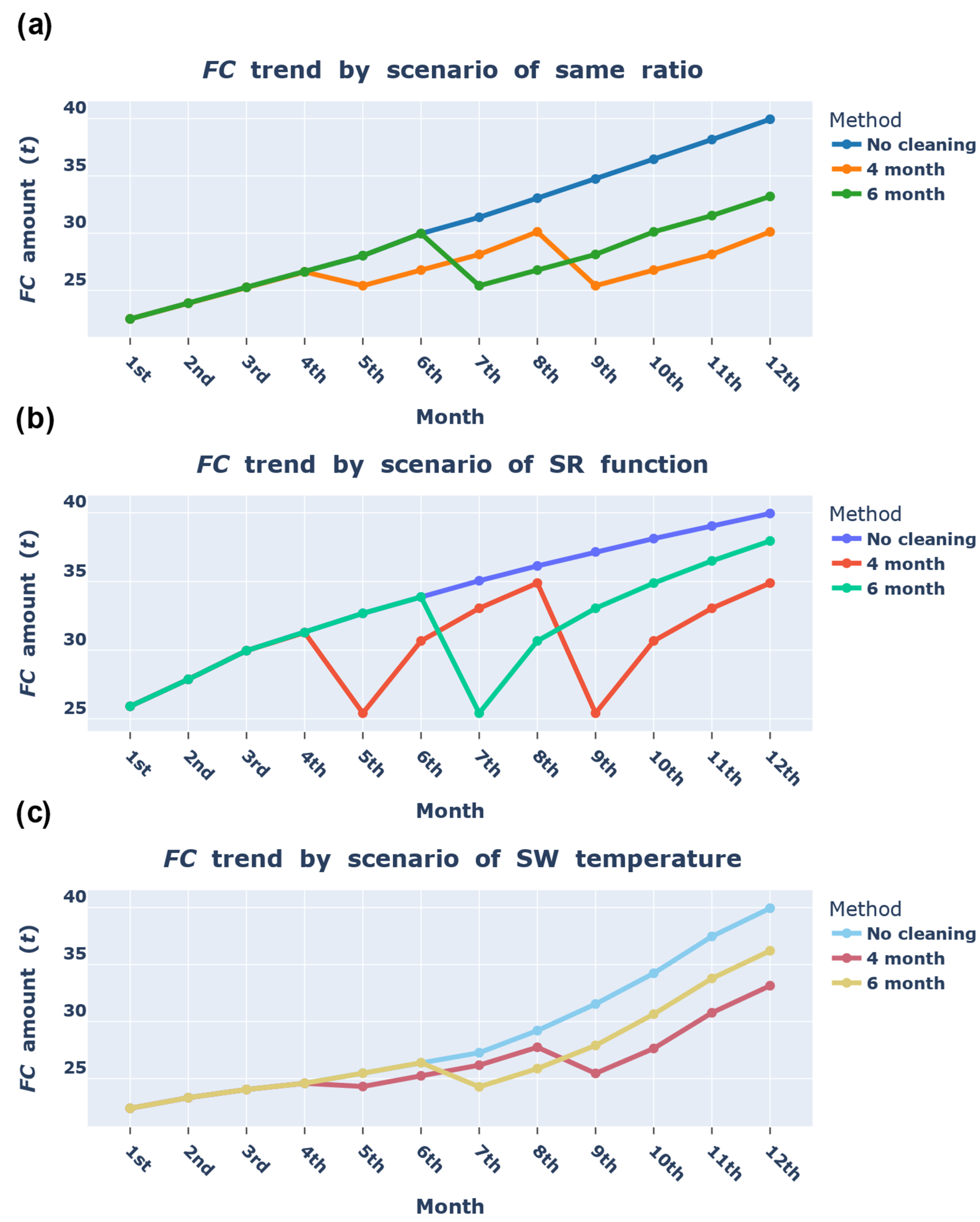
2.3.10. Calculation of FC Based on Scenarios

The shaft power was calculated and presented in Tables S4–S6 based on the ship speeds of 13 and 15 knots, and the monthly k values for all the scenarios were obtained and presented in Tables S3 and S5. The power difference was obtained from the difference between the obtained shaft power and that of the sea trial. The obtained ship speed, shaft power, and power difference values were input after min–max scaling, and the output of the optimal ANN model was inversely transformed by min–max scaling to finally obtain the FC. The monthly averaged sailing time was 53 h, and the monthly sailing time was 50 h at 13 knots and 3 h at 15 knots. Finally, the monthly FC was calculated.

3. Results

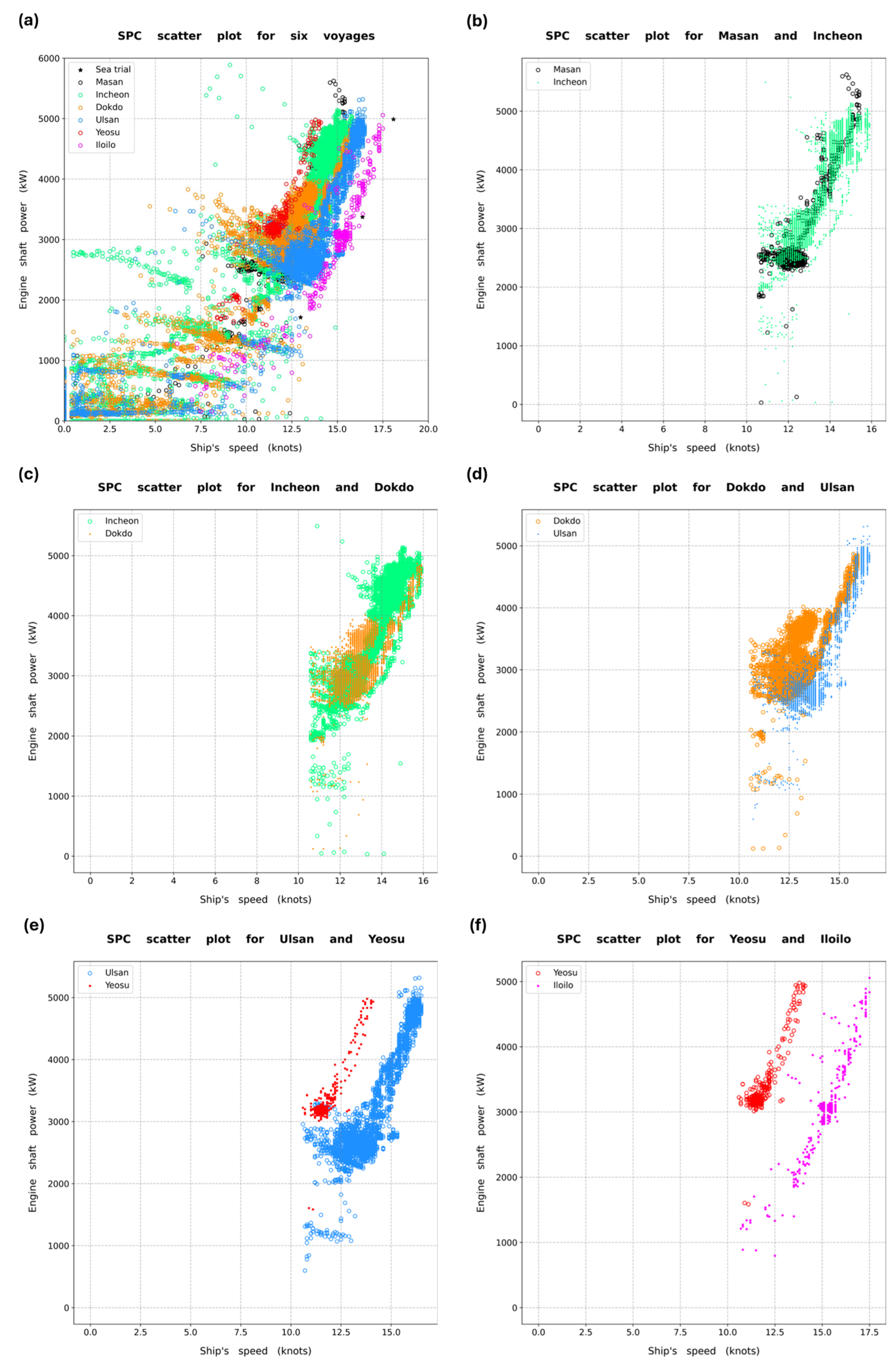
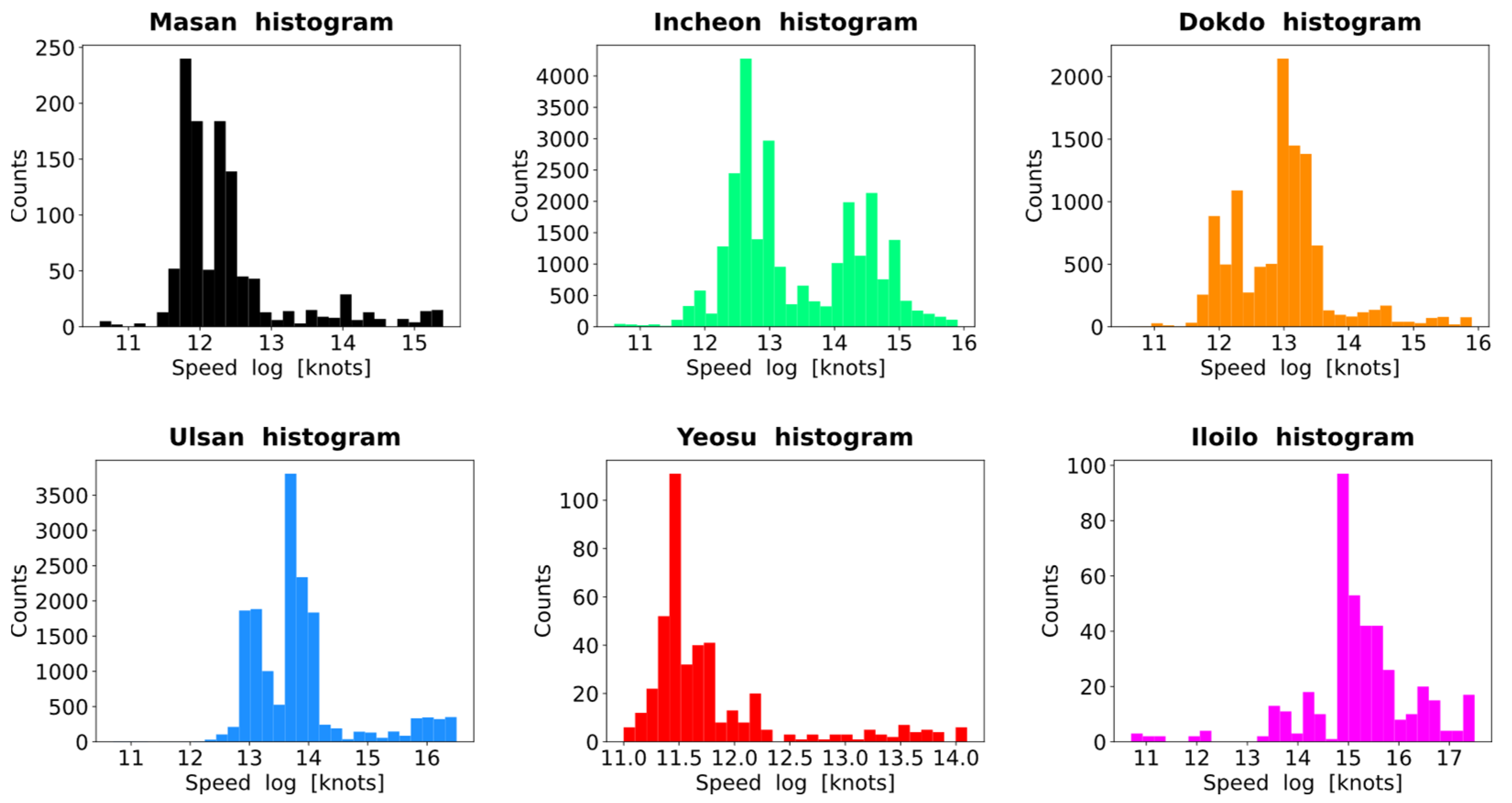
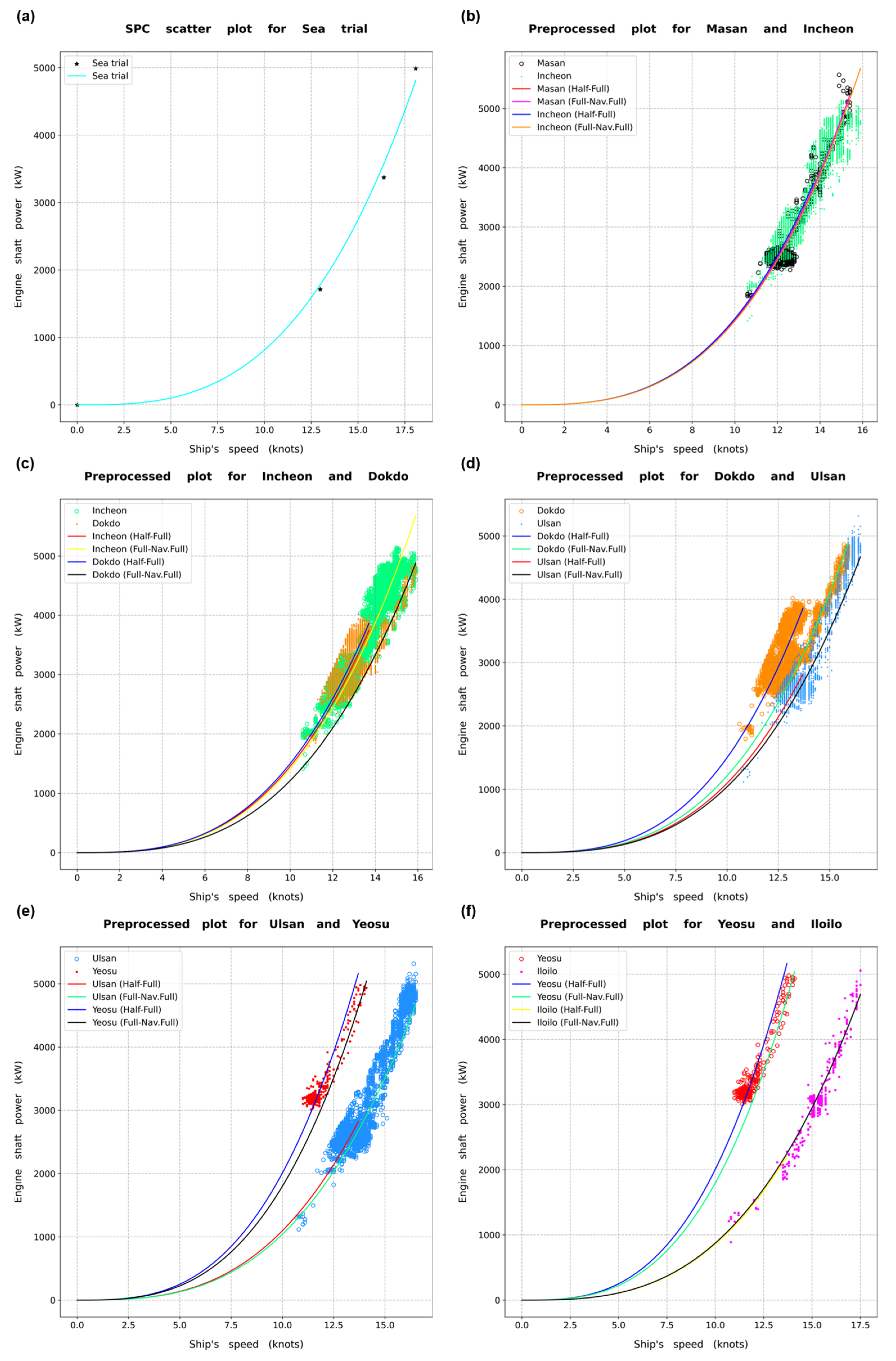
3.1. Analysis of SPC Scatter Plot for Six Voyages

Figure 5a shows that a visual analysis was difficult because of the overlapping data. Therefore, each time, two sets of voyage data were represented in the SPC scatter plots, and comparative analyses were performed according to the ship’s condition. Figure 5b shows a scatter plot of the SPC data with ship speed above 10.6 knots from the Masan and Incheon voyages. To prevent scattered data points from overlapping, the voyage datasets were represented by dots and circles. As shown in Figure 5b, the SPC data appeared to satisfy the cubic law, which can be confirmed in all the voyages (referring to Figure 5a). Most data generally followed the cubic law, with some outliers. Therefore, preprocessing became necessary to remove the outliers for proper data learning. Although a one-month gap existed between the Masan and Incheon voyages, the distributions of their SPC data exhibited a similar pattern, thus indicating that the marine life attachment over this one-month gap did not cause serious performance deterioration. Referring to Figure 5c, the outliers occurred at low shaft power values, and it happened in all six voyage datasets. In the telegraph order range from half (10.6 knots) to full (13.8 knots), the two voyage datasets showed similar distributions. However, in the full (13.8 knots) to nav. full (18.8 knots) section, the shaft power required for the Dokdo voyage to achieve the same ship speed was less than that of the Incheon voyage. This can be inferred to be the benefit of propeller polishing performed before starting the Dokdo voyage. Referring to Figure 5d, the two voyage datasets showed clear differences in distribution. In all ship speed sections, the Ulsan voyage data were generally lower than the Dokdo voyage data. This data pattern could be inferred to be the result of the UHPC conducted a month before the start of the Ulsan voyage. These results indicate that not only the propeller polishing but also underwater hull cleaning can be clearly effective over various speed ranges. Figure 5e reveals a clear difference in the distribution between the two voyage datasets. A one-year gap existed between the Yeosu and Ulsan voyages, and no underwater cleaning was performed during this period. Therefore, Yeosu voyage data were located at the uppermost left side, as shown in Figure 5a, indicating that a large amount of marine life was attached to the ship. Therefore, to improve the performance of the ship, removing the marine life attached to the hull through underwater cleaning or drydock cleaning was necessary. Figure 5f shows the clearest distribution difference among all the voyage datasets, which can also be confirmed from Figure 5a. The Iloilo voyage was conducted after the drydock cleaning, and when compared with Yeosu voyage data that did not undergo any cleaning for a year, the effect of drydock cleaning was confirmed.

3.2. Outlier Removal and Normalization

The k values in Table 6 were used to remove outliers. Methods for removing the outliers vary among users. In this study, an additional two cubic law lines were created, bordering 20% above and below the k value for each voyage, and data located outside the additional cubic law lines were removed. For example, two cubic law lines for the half–full section of the Masan voyage were obtained as follows: The values 1.137 and 1.7054, which are 20% lower and higher than 1.4212, respectively, were calculated and applied to Equation (7) to generate two cubic lines. Speed–power data points deviating from the two cubic law lines at the corresponding speed were considered outliers and excluded from the Pandas library. This process was performed on half–full and full–nav. full sections for the six voyage datasets. The preprocessed voyage data used for ANN model training are shown as SPC scatter plots in Figure 7. Furthermore, the fitted cubic law lines are shown for different telegraph order sections.
The data from which the outliers were removed were divided into training, validation, and test sets to be used in the ANN model, and the ratio was set to 6/2/2. The training, validation, and test sets of the six voyage datasets were combined to create total sets. The total sets were normalized to convert the variable values between 0 and 1 using the min–max scaling in Equation (11) to improve the model’s training performance:
x s c a l e d = x x m i n x m a x x m i n

3.3. Hyperparameter Optimization for ANN

As shown in Figure 8, values less than 40 were mostly tested for ‘batch_size’, values of 0.2 and 0.3 were mainly tested for ‘drop_rate’, a value of 1 was mainly tested for ‘hidden_layers’, and a wide distribution of values was tested for the remaining hyperparameters. Most M A E values were between 5 and 25. Although the number of hyperparameters was the largest at 8, the maximum M A E value was 69.598. As a result of hyperparameter tuning optimization, the values selected for ‘batch_size’, ‘activation’, ‘drop_rate’, ‘hidden_layers’, ‘init_mode’, ‘learning_rate’, ‘num_neurons’, and ‘optimizer’ were 8, selu, 0.1, 1, he_uniform, 0.05, 15, and adam, respectively, and the optimized M A E was 9.596.

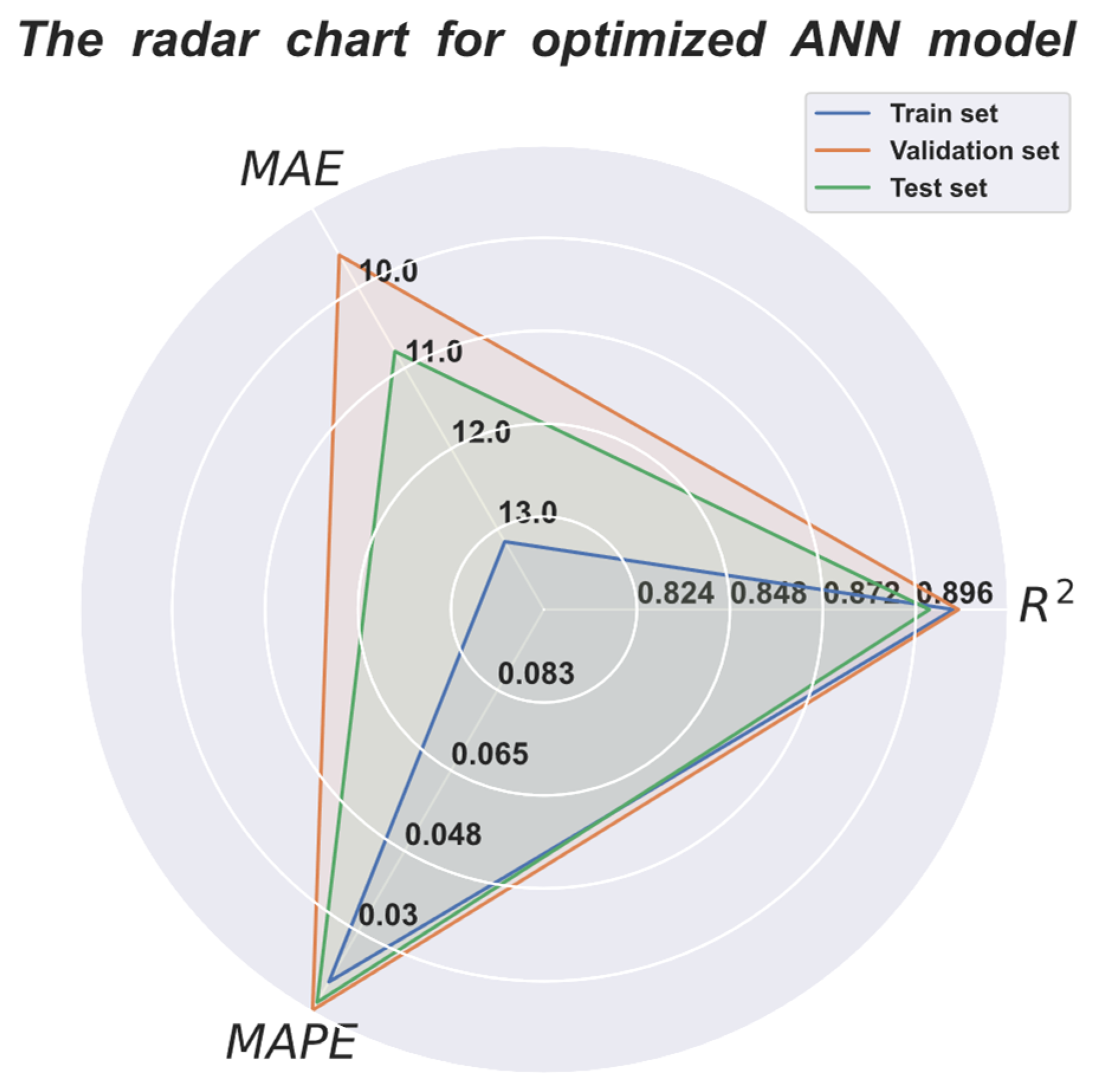
3.4. Evaluation of ANN Model Based on Performance Metrics

The performance of the model with the optimal hyperparameters was analyzed. M A E , R 2 , and M A P E were used as performance metrics, and the model performances were evaluated on the training, validation, and test sets. To facilitate a visual comparison and analysis of the model performances, a radar chart is presented in Figure 9. M A E and M A P E had small values located outside the circle, whereas R 2 had large values outside the circle. Accordingly, the larger the size of the triangle in the radar chart, the better the model’s performance.
The radar chart of the ANN model exhibited a high prediction performance for the validation set, which indicates that the ANN model had a high generalization performance and was not extremely overfitted to the training set. It can be inferred that this was due to the use of an early stopping function and dropout among the hyperparameters. The performance metrics of the ANN model are listed in Table 10. Based on the results, the optimized ANN model had high performance on the validation and test sets for FC prediction.

4. Scenario-Based Economic Analysis

To analyze the economic impact based on the calculated monthly FC, the LSMGO prices at the international ports of Rotterdam and Singapore were referenced, as presented in Table 11 [49,50]. The fuel prices at these two ports are typically representative of the global prices.
Based on the monthly FC obtained from Tables S4–S6 and the fuel prices from Table 11, the monthly FC costs were obtained, as shown in Table S7. Referring to Table S7, the change in the monthly FC differed according to the three scenarios and, consequently, the monthly FC costs as well. As a result, there were differences in the total FC and costs between the three scenarios.
The standard method suggested by the Korean Register shows that the in-water survey is conducted once every 2.5 years and the docking survey is conducted once every 5 years [51]. During the underwater survey, underwater hull cleaning is typically performed in advance to facilitate the inspection. Referring to Akinfiev et al., the fuel performance decreased six months after the drydock and continued to decrease rapidly [52]. Accordingly, it is recommended that large vessels perform underwater hull cleaning earlier than 2.5 years, typically at intervals of 4–6 months between the hull cleanings. Furthermore, it is recommended that hull cleaning be performed thrice a year for certain geographic fouling zones established by the U.S. Navy. Therefore, this study conducted an analysis to establish the economic feasibility of UHPC over four- and six-month cycles. The cost incurred for UHPC was calculated to be USD 7500, according to past work history and reference data [53].
Referring to Table S8, the UHPC was performed in the 5th and 9th months and the k value of the Ulsan voyage from Table 6 was applied. After the k value decreased, it increased again by the monthly increase amount specified in Table 8. Table S9 shows the monthly FC when UHPC was performed every six months. The monthly FC values in Tables S10–S13 were calculated in the same manner as in Tables S8 and S9 by changing the k values reffering to Table 8, except for the scenario of ‘SW temperature’. As the k value of the Ulsan voyage was obtained one month after a UHPC, the increase in the k value for October (Table S2) was subtracted from the k value of the Ulsan voyage. Based on the subtracted k value, the k value increase from the 5th and 9th months was applied in the UHPC with a 4-month cycle, and the k value increase from the 7th month was applied in the 6-month cycle.
Figure 10 shows the FC trend for each of the three scenarios, allowing a comparison of the effects of UHPC. In the case of the ‘same ratio’ scenario, the FC increased at a constant rate with no cleaning, and after the UHPC as well. For the 7th to 8th month period, it appears that the gaps between the three graphs were of similar size. However, for the 9th to 12th month period, the gap between ‘no cleaning’ and ‘four-month cycle’ was twice as large as that between the ‘four-month cycle’ and ‘six-month cycle’. This is because the UHPC was performed twice in a four-month cycle, indicating that the effect of periodic UHPC increased as time passed compared with ‘no cleaning’. In the case of the ‘SR function’ scenario, the FC increased in the shape of an SR graph. Here, the reason FC decreased sharply after the UHPC was that the initial increase in the value was large because of the nature of the SR graph. In other words, the effect was maximized at the beginning of the UHPC implementation compared with that of the ‘no cleaning’ case, and the effect became smaller over time. In the ‘SW temperature’ scenario, the increase in the FC was small from the 1st to the 4th month because this period coincided with winter. Therefore, the decrease in the FC appeared to be smaller in the 5th month than in the 7th or 9th month. The increase in the FC was large from the 9th to the 12th month, when percent cover of the five species on the experimental panel was large, according to the referred research. In other words, the effectiveness of the UHPC in the ‘SW temperature’ scenario might vary depending on the season of its implementation.
The fuel costs based on the monthly FCs in Tables S8–S13 were calculated according to the UHPC interval, as shown in Tables S14 and S15. The difference in the total value between Tables S14 and S15 and Table S7 was calculated as the saving from the UHPC. In calculating the fuel cost saving, USD 15,000 and USD 7500 were reflected in Tables S14 and S15, respectively, because those tables contained two UHPCs and one UHPC, respectively. A summary of Tables S14 and S15 is shown in Figure 11 and Figure 12 and is separated into left and right by the UHPC interval.
The blue and black line graphs are the monthly averaged fuel costs without UHPC. This shows that the fuel cost to be spent every month increased for all the scenarios, and the fuel prices in Rotterdam were higher than those in Singapore. The green and red line graphs represent the monthly averaged fuel costs based on the UHPC interval. The line graph is expressed as the FC multiplied by the fuel cost; thus, it shows the same trend as does Figure 10. A candle chart is displayed using the minimum and maximum values from Tables S14 and S15. Referring to the left candle charts in Figure 11, the maximum values of the candle charts exceeded the monthly averaged fuel cost without UHPC before the 9th month of the UHPC. However, it appears that the maximum values were generally lower than the monthly averaged fuel cost with no UHPC after the 9th month of the UHPC. Particularly, the effect of the second UHPC in the four-month cycle was maximized in the ‘same ratio’ scenario. Referring to the candle charts on the right, the maximum values after the 7th month of the UHPC were similar to or slightly higher than the monthly averaged fuel cost during no UHPC. However, the effect of UHPC appeared to be clear in terms of fuel cost savings, as indicated by the green and red line graphs for both UHPC intervals [47].
Figure 12 shows the bar charts of the saving accrued by subtracting the UHPC cost from the one-year fuel cost saving. The bar charts are based on the average fuel cost saving, and the error bars are based on the maximum and minimum fuel cost savings. On a one-year basis, Rotterdam and Singapore’s fuel cost savings were similar. By comparing the effects of the UHPC interval, it appears that cleaning the four-month UHPC cycle can further reduce the fuel cost. Particularly, the difference in fuel cost saving according to the UHPC interval was significant in the ‘SR function’ scenario. In the ‘same ratio’ scenario, the Rotterdam fuel cost saving was the highest at USD 26,685 and USD 24,102 for the four- and six-month UHPC intervals, respectively. In the ‘SW temperature’ scenario, Singapore’s fuel cost saving was the lowest at USD 10,402 and USD 9653 for the four- and six-month UHPC intervals, respectively.
In this study, the hull cleaning interval was set to four and six months; however, various intervals could be analyzed depending on the user, thus making it possible to determine the optimal hull cleaning timing, considering the sailing schedule and hull cleaning cost. Additionally, the proposed methodology has the advantage of deriving stable results by adopting the conservative approach by referring to various scenarios and fuel prices.

5. Discussion

As of 2023, the world’s merchant fleet consisted of 105,493 vessels of 100 gross tons and above, and as of 2020, the number of world’s fishing vessels was estimated at 4.1 million [54,55]. As all these vessels float on water, avoiding biofouling can be an impossible task. Therefore, proper physical biofouling removal methods are performed to remove biofouling.
Powered rotary brush cleaning is performed by divers to remove biofouling. However, hull cleaning by divers has disadvantages in terms of accident risk [56]. Furthermore, rotary brush cleaning can damage hull welds and protrusions and reduce mechanical integrity. In addition to underwater cleaning performed in ports, biofouling from ships is regularly removed during drydocking using methods, such as hydroblasting, sand blasting, scrapping, or sandpapering [57]. However, implementing the physical biofouling removal methods require enormous costs. Therefore, proper management of biofouling is essential from an economic perspective.
As recently built ships are equipped with more intelligence, the biofouling management framework presented in this study, which is based on collected data, can be applied. However, this does not mean that it cannot be applied to existing merchant or oceangoing fishing vessels. This is because the engine logbooks of these ships are updated daily by skilled marine engineers, and manually written values, such as the ship speed, shaft power, and fuel consumption values, can be transformed into a Microsoft Excel files for data preprocessing. Furthermore, the date when the UHPC was performed is recorded in the engine logbook, and all ships possess sea trial data. Therefore, an FC prediction AI model that represents the characteristics of each ship can be developed based on sea trial data, UHPC history, and the Excel file, in which the ship’s performance variables are written. If a company that owns a ship cannot analyze the data or develop an AI model, it can use the framework developed by a ship management software company. Thus, most ships worldwide can accrue economic benefit from optimal UHPC management plans.
Our research presented a novel framework for calculating coefficients based on ship big data and analyzed the economic impact based on various scenarios, UHPC costs, and AI model results; accordingly, follow-up research can be conducted using this approach. Referring to the Figure 12, the annual fuel cost savings were USD 10,402–26,685 and USD 9653–24,102 when UHPC intervals were four and six months, respectively. Although annual fuel cost savings may vary depending on the price of fuel and UHPC, shipping companies could select optimal UHPC intervals based on the framework we have presented.
The framework can be applied to all existing ships, and offers a solution based on data science without requiring additional expensive equipment or sensors. Therefore, the problem of performance degradation caused by biofouling of commercial ships and fishing boats floating in the world’s oceans can be effectively addressed. This can potentially guide ships worldwide in reducing their fuel consumption by performing economically effective UHPC, and achieving net zero emissions, as targeted.

6. Conclusions

Data and ship-cleaning history were obtained from the latest training ship that had performed six voyages. The measured parameters ‘speed log’ and ‘shaft power’ were used as input variables, and fuel consumption was used as an output variable to train the ANN model. We performed novel feature engineering that could reflect the state of the underwater structure to generate ‘power difference’ data and use them as an input variable.
The data were selected at a ship speed of 10.6 knots or higher and were divided into half–full and full–nav. full sections in telegraph order. Therefore, the proposed curve-fitting procedure was limited to the higher-speed range. The coefficient values of a sea trial and six voyages were obtained using a curve-fitting algorithm, and outliers were removed.
The speed–power curve scatter plots of the six voyages were compared and analyzed based on the cleaning history and data distribution. The W&B library was used to optimize various hyperparameters of the ANN algorithm, and the Bayesian optimization process was confirmed using a parallel coordinate plot. The ANN algorithm exhibited high prediction and generalization performance for predicting the fuel consumption.
Scenario-based economic analysis was conducted to verify the effectiveness of UHPC and determine the optimal hull cleaning timing. Three scenarios were created, in which the coefficient changed based on ‘same ratio’, ‘SR function’, and ‘SW temperature’ using data that did not include underwater cleaning for a year. Based on the distribution of the ship operation data, the speeds for half–full and full–nav. full sections were determined. The monthly fuel consumption for each scenario was calculated based on the optimized ANN model and the monthly vessel operation time.
The fuel costs for four- and six-month UHPC intervals were calculated using monthly fuel consumption and low-sulfur marine gas oil prices from two international ports. The annual fuel cost savings were calculated from the one-year fuel costs incurred with and without UHPC being performed, and these were presented as candle and line charts; for comparison, the cost when UHPC was not implemented was shown as a line chart. The results confirmed that the monthly fuel costs decreased for either of the UHPC intervals. Particularly, for the four-month cycle, the fuel cost saving was found to be greater. Yearly fuel cost savings of USD 10,402–26,685 and USD 9653–24,102 were achieved with four- and six-month UHPC cycles, respectively. Ship management companies can determine the optimal hull cleaning timing by considering various UHPC intervals and hull cleaning costs.

Supplementary Materials

The following supporting information can be downloaded at: https://www.mdpi.com/article/10.3390/jmse13050952/s1. Table S1: Monthly k for the ‘same ratio’ scenario. Table S2: Monthly percent cover value according to Busan seawater (SW) temperature and monthly increase in k . Table S3: Monthly k for the ‘SR function’ and ‘SW temperature’ scenarios. Table S4: Calculation of monthly FC based on ‘same ratio’ scenario. Table S5: Calculation of monthly FC based on ‘SR function’ scenario. Table S6: Calculation of monthly FC based on ‘SW temperature’ scenario. Table S7: Fuel costs for the three scenarios considered, according to the bunker prices at two international ports. Table S8: Monthly FC calculations for the ‘same ratio’ scenario with a 4-month UHPC cycle. Table S9: Monthly FC calculation for the ‘same ratio’ scenario with a 6-month UHPC cycle. Table S10: Monthly FC calculation for the ‘SR function’ scenario, with a 4-month UHPC cycle. Table S11: Monthly FC calculation for the ‘SR function’ scenario, with a 6-month UHPC cycle. Table S12: Monthly FC calculation for the ‘SW temperature’ scenario, with a 4-month UHPC cycle. Table S13: Monthly FC calculation for the ‘SW temperature’ scenario, with a 6-month UHPC cycle. Table S14: Fuel cost savings for the three scenarios considered, with a 4-month UHPC cycle. Table S15: Fuel cost savings for the three scenarios considered, with a 6-month UHPC cycle.

Author Contributions

Conceptualization, M.-H.P., J.-J.H., G.-H.Y. and W.-J.L.; methodology, M.-H.P., J.-J.H. and G.-H.Y.; data curation, M.-H.P., J.-J.H. and G.-H.Y.; investigation, M.-H.P.; formal analysis, M.-H.P.; software, M.-H.P.; visualization, M.-H.P. and J.-J.H.; supervision, W.-J.L.; project administration, W.-J.L.; funding acquisition, W.-J.L.; writing—original draft, M.-H.P.; writing—review and editing, M.-H.P. and W.-J.L. All authors have read and agreed to the published version of the manuscript.

Funding

This research was supported by the ‘Autonomous Ship Technology Development Program (20016140)’, funded by the Ministry of Trade, Industry, and Energy (MOTIE, Korea) and the Korea Planning and Evaluation Institute of Industrial Technology (KEIT), the National Research Foundation of Korea (NRF) grant, funded by the Korea government (MSIT; NRF-2022R1F1A1073764), and the ‘Technology development Program (S3366238)’, funded by the Ministry of SMEs and Startups (MSS, Korea).

Data Availability Statement

The original contributions presented in this study are included in the article. Further inquiries can be directed to the corresponding author.

Conflicts of Interest

The authors declare no conflicts of interest.

Nomenclature

AIArtificial intelligence
ANNArtificial neural network
FCFuel consumption
IMOInternational Maritime Organization
ISOInternational Organization for Standardization
KHOAKorea Hydrographic and Oceanographic Agency
KRISOKorea Research Institute of Ships and Ocean Engineering
LMLevenberg–Marquardt
LSMGOLow-sulfur marine gas oil
MAEMean absolute error
MAPEMean absolute percentage error
M/EMain engine
ReLURectified linear unit
RMSERoot mean square error
RPMRevolutions per minute
SPCSpeed–power curve
SRSquare root
SWSea water
UHPCUnderwater hull and propeller cleaning
UKUnited Kingdom
W&BWeights and biases

References

  1. Lindholdt, A.; Dam-Johansen, K.; Olsen, S.M.; Yebra, D.M.; Kiil, S. Effects of Biofouling Development on Drag Forces of Hull Coatings for Ocean-Going Ships: A Review. J. Coat. Technol. Res. 2015, 12, 415–444. [Google Scholar] [CrossRef]
  2. Adland, R.; Cariou, P.; Jia, H.; Wolff, F.C. The Energy Efficiency Effects of Periodic Ship Hull Cleaning. J. Clean. Prod. 2018, 178, 1–13. [Google Scholar] [CrossRef]
  3. Oliveira, D.R.; Granhag, L. Ship Hull In-Water Cleaning and Its Effects on Fouling-Control Coatings. Biofouling 2020, 36, 332–350. [Google Scholar] [CrossRef]
  4. Demirel, Y.K.; Turan, O.; Incecik, A. Predicting the Effect of Biofouling on Ship Resistance Using CFD. Appl. Ocean Res. 2017, 62, 100–118. [Google Scholar] [CrossRef]
  5. Oliveira, D.; Larsson, A.I.; Granhag, L.; Ralston, E.; Gardner, H.; Hunsucker, K.Z.; Swain, G.; Schultz, M.P.; Tian, L.; Yin, Y.; et al. Factors That Influence Vessel Biofouling and Its Prevention and Management; Final Report for CEBRA Project 190803; Cebra: Parkville, Australia, 2021; p. 34. [Google Scholar]
  6. Hakim, M.L.; Nugroho, B.; Nurrohman, M.N.; Suastika, I.K.; Utama, I.K.A.P. Investigation of Fuel Consumption on an Operating Ship Due to Biofouling Growth and Quality of Anti-Fouling Coating. IOP Conf. Ser. Earth Environ. Sci. 2019, 339, 012037. [Google Scholar] [CrossRef]
  7. Valchev, I.; Coraddu, A.; Kalikatzarakis, M.; Geertsma, R.; Oneto, L. Numerical Methods for Monitoring and Evaluating the Biofouling State and Effects on Vessels’ Hull and Propeller Performance: A Review. Ocean Eng. 2022, 251, 110883. [Google Scholar] [CrossRef]
  8. Liu, S.; Kee, Y.H.; Shang, B.; Papanikolaou, A. Assessment of the Economic, Environmental and Safety Impact of Biofouling on a Ship’s Hull and Propeller. Ocean Eng. 2023, 285, 115481. [Google Scholar] [CrossRef]
  9. Swain, G.; Erdogan, C.; Foy, L.; Gardner, H.; Harper, M.; Hearin, J.; Hunsucker, K.Z.; Hunsucker, J.T.; Lieberman, K.; Nanney, M.; et al. Proactive In-Water Ship Hull Grooming as a Method to Reduce the Environmental Footprint of Ships. Front. Mar. Sci. 2022, 8, 808549. [Google Scholar] [CrossRef]
  10. Song, C.; Cui, W. Review of Underwater Ship Hull Cleaning Technologies. J. Mar. Sci. Appl. 2020, 19, 415–429. [Google Scholar] [CrossRef]
  11. Oliveira, D.R.; Lagerström, M.; Granhag, L.; Werner, S.; Larsson, A.I.; Ytreberg, E. A Novel Tool for Cost and Emission Reduction Related to Ship Underwater Hull Maintenance. J. Clean. Prod. 2022, 356, 131882. [Google Scholar] [CrossRef]
  12. Coraddu, A.; Lim, S.; Oneto, L.; Pazouki, K.; Norman, R.; Murphy, A.J. A Novelty Detection Approach to Diagnosing Hull and Propeller Fouling. Ocean Eng. 2019, 176, 65–73. [Google Scholar] [CrossRef]
  13. Coraddu, A.; Oneto, L.; Baldi, F.; Cipollini, F.; Atlar, M.; Savio, S. Data-Driven Ship Digital Twin for Estimating the Speed Loss Caused by the Marine Fouling. Ocean Eng. 2019, 186, 106063. [Google Scholar] [CrossRef]
  14. Farkas, A.; Degiuli, N.; Martić, I.; Ančić, I. Energy Savings Potential of Hull Cleaning in a Shipping Industry. J. Clean. Prod. 2022, 374, 134000. [Google Scholar] [CrossRef]
  15. Laurie, A.; Anderlini, E.; Dietz, J.; Thomas, G. Machine Learning for Shaft Power Prediction and Analysis of Fouling Related Performance Deterioration. Ocean Eng. 2021, 234, 108886. [Google Scholar] [CrossRef]
  16. Cesium The Platform for 3D Geospatial. Available online: https://cesium.com/ (accessed on 1 April 2025).
  17. Archnuri Completion of Basic Design for Construction of New Training Ship Hannara. Available online: http://www.archnuri.com/new/sub01.asp?mode=list&page=33&s_type=&s_value=&n_code=ARCHNURI-201201&c_code=02&c_sort=0201 (accessed on 1 April 2025).
  18. Amato, F.; López, A.; Peña-Méndez, E.M.; Vaňhara, P.; Hampl, A.; Havel, J. Artificial Neural Networks in Medical Diagnosis. J. Appl. Biomed. 2013, 11, 47–58. [Google Scholar] [CrossRef]
  19. Villarrubia, G.; De Paz, J.F.; Chamoso, P.; De la Prieta, F. Artificial Neural Networks Used in Optimization Problems. Neurocomputing 2018, 272, 10–16. [Google Scholar] [CrossRef]
  20. Park, M.-H.; Hur, J.-J.; Lee, W.-J. Prediction of Diesel Generator Performance and Emissions Using Minimal Sensor Data and Analysis of Advanced Machine Learning Techniques. J. Ocean Eng. Sci. 2023, 10, 150–168. [Google Scholar] [CrossRef]
  21. Park, M.H.; Lee, C.M.; Nyongesa, A.J.; Jang, H.J.; Choi, J.H.; Hur, J.J.; Lee, W.J. Prediction of Emission Characteristics of Generator Engine with Selective Catalytic Reduction Using Artificial Intelligence. J. Mar. Sci. Eng. 2022, 10, 1118. [Google Scholar] [CrossRef]
  22. Jiang, J.; Trundle, P.; Ren, J. Medical Image Analysis with Artificial Neural Networks. Comput. Med. Imaging Graph. 2010, 34, 617–631. [Google Scholar] [CrossRef]
  23. Park, M.H.; Hur, J.J.; Lee, W.J. Prediction of Oil-Fired Boiler Emissions with Ensemble Methods Considering Variable Combustion Air Conditions. J. Clean. Prod. 2022, 375, 134094. [Google Scholar] [CrossRef]
  24. SciPy v1.12.0 Manual Scipy.Optimize.Curve_fit. Available online: https://docs.scipy.org/doc/scipy/reference/generated/scipy.optimize.curve_fit.html (accessed on 1 April 2025).
  25. Chen, K.; Zhang, M.; Fu, S.; Zhao, B.; Luo, C. A Numerical Model for Stress Relaxation Analysis of Sealing Systems in Nonbonded Pipe End Fittings. J. Ocean Eng. Sci. 2023, 2, 43. [Google Scholar] [CrossRef]
  26. Shan, S. A Levenberg-Marquardt Method for Large-Scale Bound-Constrained Nonlinear Least-Squares. Ph.D. Thesis, University of British Columbia, Vancouver, BC, Canada, 2008. [Google Scholar]
  27. Wang, M.; Xu, X.; Yan, Z.; Wang, H. An Online Optimization Method for Extracting Parameters of Multi-Parameter PV Module Model Based on Adaptive Levenberg-Marquardt Algorithm. Energy Convers. Manag. 2021, 245, 114611. [Google Scholar] [CrossRef]
  28. Gavin, H.P. The Levenberg-Marquardt Algorithm for Nonlinear Least Squares Curve-Fitting Problems; Duke University: Durham, NC, USA, 2019. [Google Scholar]
  29. Dkhichi, F.; Oukarfi, B.; Fakkar, A.; Belbounaguia, N. Parameter Identification of Solar Cell Model Using Levenberg-Marquardt Algorithm Combined with Simulated Annealing. Sol. Energy 2014, 110, 781–788. [Google Scholar] [CrossRef]
  30. Furuno Electric. Finished Plan—Speed Log (DS-60); Furuno Electric: Nishinomiya, Hyogo, Japan, 2019. [Google Scholar]
  31. Aquametro. Final Drawing—Flowmeter for M/E F.O (10K-40A); Aquametro: Therwil, Switzerland, 2018. [Google Scholar]
  32. Specs. Final Drawing for Shaft Torque Power Meter; Specs: Austin, TX, USA, 2018. [Google Scholar]
  33. Psaraftis, H.N.; Lagouvardou, S. Ship Speed vs Power or Fuel Consumption: Are Laws of Physics Still Valid? Regression Analysis Pitfalls and Misguided Policy Implications. Clean. Logist. Supply Chain 2023, 7, 100111. [Google Scholar] [CrossRef]
  34. Park, M.H.; Yeo, S.; Yang, S.K.; Shin, D.; Kim, J.H.; Choi, J.H.; Lee, W.J. Analysis and Forecasting of National Marine Litter Based on Coastal Data in South Korea from 2009 to 2021. Mar. Pollut. Bull. 2023, 189, 114803. [Google Scholar] [CrossRef]
  35. Renaud, O.; Victoria-Feser, M.P. A Robust Coefficient of Determination for Regression. J. Stat. Plan. Inference 2010, 140, 1852–1862. [Google Scholar] [CrossRef]
  36. Aydın, B.; Yağuzluk, S.; Açıkkar, M. Prediction of Landslide Tsunami Run-up on a Plane Beach through Feature Selected MLP-Based Model. J. Ocean Eng. Sci. 2024, 9, 222–231. [Google Scholar] [CrossRef]
  37. Keras. Keras 3 API Documentation. Available online: https://keras.io/api/ (accessed on 1 April 2025).
  38. Weights & Biases. The AI Developer Platform. Available online: https://wandb.ai/site (accessed on 1 April 2025).
  39. Wu, J.; Chen, X.Y.; Zhang, H.; Xiong, L.D.; Lei, H.; Deng, S.H. Hyperparameter Optimization for Machine Learning Models Based on Bayesian Optimization. J. Electron. Sci. Technol. 2019, 17, 26–40. [Google Scholar] [CrossRef]
  40. Visscher, J.P. Nature and Extent of Fouling of Ships’ Bottoms. Bull. Bur. Fish. Part II 1927, 43, 193–252. [Google Scholar]
  41. Hadžić, N.; Gatin, I.; Uroić, T.; Ložar, V. Biofouling Dynamic and Its Impact on Ship Powering and Dry-Docking. Ocean Eng. 2022, 245, 110522. [Google Scholar] [CrossRef]
  42. Munk, T.; Kane, D.; Yebra, D.M. The Effects of Corrosion and Fouling on the Performance of Ocean-Going Vessels: A Naval Architectural Perspective. In Advances in Marine Antifouling Coatings and Technologies; Elsevier: Amsterdam, The Netherlands, 2009. [Google Scholar]
  43. Graham, H.W.; Gay, H. Season of Attachment and Growth of Sedentary Marine Organisms at Oakland, California. Ecology 1945, 26, 375–386. [Google Scholar] [CrossRef]
  44. Lord, J.P.; Calini, J.M.; Whitlatch, R.B. Influence of Seawater Temperature and Shipping on the Spread and Establishment of Marine Fouling Species. Mar. Biol. 2015, 162, 2481–2492. [Google Scholar] [CrossRef]
  45. UK Defence Club. Hull Fouling: The Legal and the Practical. Available online: https://www.ukdefence.com/fileadmin/uploads/uk-defence/Documents/Soundings/2020/1411-UKDC-Hull-Fouling-web.pdf (accessed on 1 April 2025).
  46. Crisp, D.J. The Effects of the Severe Winter of 1962–63 on Marine Life in Britain. J. Anim. Ecol. 1964, 33, 165. [Google Scholar] [CrossRef]
  47. Lord, J.P. Impact of Seawater Temperature on Growth and Recruitment of Invasive Fouling Species at the Global Scale. Mar. Ecol. 2017, 38, e12404. [Google Scholar] [CrossRef]
  48. KHOA. Ocean Data in Grid Framework. Available online: http://www.khoa.go.kr/oceangrid/khoa/intro.do (accessed on 1 April 2025).
  49. Ship & Bunker. World Bunker Prices. Available online: https://shipandbunker.com/prices#MGO (accessed on 1 April 2025).
  50. Bayraktar, M.; Yuksel, O.; Pamik, M. An Evaluation of Methanol Engine Utilization Regarding Economic and Upcoming Regulatory Requirements for a Container Ship. Sustain. Prod. Consum. 2023, 39, 345–356. [Google Scholar] [CrossRef]
  51. Korean Register Rules for the Classification of Steel Ships Part 1 Classification and Surveys. Available online: https://www.krs.co.kr/KRRules/KRRules2022/KRRulesE.html (accessed on 1 April 2025).
  52. Akinfiev, T.; Janushevskis, A.; Lavendelis, E. A Brief Survey of Ship Hull Cleaning Devices. Transp. Eng. 2007, 24, 133–146. [Google Scholar]
  53. GloMEEP. Hull Cleaning. Available online: https://glomeep.imo.org/technology/hull-cleaning/ (accessed on 1 April 2025).
  54. FAO. Estimate of the Global Fleet and Its Regional Distribution. Available online: https://www.fao.org/3/cc0461en/online/sofia/2022/fishing-fleet.html (accessed on 1 April 2025).
  55. UNCTAD. Review of Maritime Transport 2023. Available online: https://unctad.org/system/files/official-document/rmt2023_en.pdf (accessed on 1 April 2025).
  56. Nassiraei, A.A.F.; Sonoda, T.; Ishii, K. Development of Ship Hull Cleaning Underwater Robot. In Proceedings of the International Conference on Emerging Trends in Engineering and Technology, ICETET, Himeji, Japan, 5–7 November 2012. [Google Scholar]
  57. Soon, Z.Y.; Jung, J.H.; Yoon, C.; Kang, J.H.; Kim, M. Characterization of Hazards and Environmental Risks of Wastewater Effluents from Ship Hull Cleaning by Hydroblasting. J. Hazard. Mater. 2021, 403, 123708. [Google Scholar] [CrossRef]
Figure 1. Images of the underwater hull, propeller, and thruster before cleaning at the drydock (all parts are covered with marine life): (a) bulbous bow, (bd) underwater hull, (e) enlarged photograph of underwater hull, (f) thruster propeller seen from the front, (g) thruster propeller seen from the back, (h) sea chest grating, (i) propeller, and (j) lower hull of the bilge keel.
Jmse 13 00952 g001
Figure 2. Images of the underwater hull, propeller, and thruster during and after cleaning at the drydock: (a,b) jet cleaning of the underwater hull, (c,d) sand blasting of the underwater hull, (e) cleaning of the thruster, (f) painting of the thruster, (g) disassembled propeller after cleaning, (hj) touch-up painting with anti-corrosive paint, and (k,l) full painting with antifouling paint.
Jmse 13 00952 g002
Figure 3. Universal globe map of the destination routes sailed by T/S HANNARA [16,17].
Jmse 13 00952 g003
Figure 4. Flowchart for scenario-based analysis of the economic impact of underwater biofouling.
Jmse 13 00952 g004
Figure 7. SPC scatter plots and fitted cubic law lines for preprocessed data of sea trial and six voyages: (a) SPC scatter plot for sea trial, and preprocessed plots for (b) Masan and Incheon, (c) Incheon and Dokdo, (d) Dokdo and Ulsan, (e) Ulsan and Yeosu, and (f) Yeosu and Iloilo.
Jmse 13 00952 g007
Figure 8. Parallel coordinate plot of the ANN model for hyperparameter tuning.
Jmse 13 00952 g008
Figure 9. Radar chart based on three performance metrics for the optimized ANN model.
Jmse 13 00952 g009
Figure 10. FC trend with different cleaning methods under the three scenarios: (a) ‘same ratio’, (b) ‘SR function’, and (c) ‘SW temperature’.
Jmse 13 00952 g010
Figure 11. Fuel cost trends for different scenarios and UHPC intervals: (a) ‘same ratio’, 4 months; (b) ‘same ratio’, 6 months; (c) ‘SR function’, 4 months; (d) ‘SR function’, 6 months; (e) ‘SW temperature’, 4 months; (f) ‘SW temperature’, 6 months.
Jmse 13 00952 g011
Figure 12. Yearly fuel cost savings for different scenarios and UHPC intervals: (a) four-month UHPC cycle and (b) six-month UHPC cycle.
Jmse 13 00952 g012
Table 1. Key specifications of the training ship.
ParameterValueParameterValue
IMO number9,807,279Length between perpendiculars (m)120
NameHANNARABreadth (m)19.4
TypeTraining shipWetted surface area (m2)2694.8
FlagSouth KoreaYear built2019
Gross tonnage (t)9196Engine typeMAN 6S40ME-B9.5
Summer deadweight (t)3671Engine power6618 kW at 146 rpm
Displacement at maximum draught (t)9122.2No. of propeller blades4
Length overall (m)133Propeller diameter (m)4
Table 2. Description of ship cleaning history for six voyages.
Voyage DestinationDate of Data CollectionDescription
Masan25–26 April 2022Two months before bow/stern thrusters’ cleaning and propeller polishing.
Incheon25–30 May 2022One month before bow/stern thrusters’ cleaning and propeller polishing.
Dokdo25–27 June 2022After bow/stern thrusters’ cleaning and propeller polishing (23 June 2022).
Ulsan31 October–3 November 2022(1) Two months after stern thruster cleaning (24 August 2022).
(2) One month after underwater hull and propeller cleaning (30 September 2022).
Yeosu16 October 2023Before drydocking.
Iloilo11 November 2023After drydocking.
Table 3. Information on paint used at the drydock for hull and propeller coatings.
Painting AreaPaint NamePaint MakerPaint TypeDry Film Thickness (µm)Thinner NumberOrder of Painting
Upper part for the waterline of hullEH2350-2260KCC CorporationEpoxy anti-abrasion1000241st
EH2350-1128Epoxy anti-abrasion1000242nd
UT6581(K1)-1000Polyurethane finish10006243rd
Lower part for the waterline of hullEH2350-2260Epoxy anti-abrasion1000241st
EH2560-Y/LIGHTModified vinyl epoxy1000242nd
A/F795-RED BROWNTin-free SPC antifouling paint1000023rd
PropellerEH2350-2260Epoxy anti-abrasion1250241st
MetaCruise PrimerEpoxy primer1250242nd
MetaCruise TieTie coat1000023rd
MetaCruise NSSilicone AF150Not recommended4th
Table 4. Specifications of fuel oil flowmeter, shaft torque power meter, and Doppler sonar [30,31,32].
Fuel Oil FlowmeterShaft Torque Power MeterDoppler Sonar
ItemDescriptionItemDescriptionItemDescription
ManufacturerAquametroManufacturerSpecsManufacturerFuruno Electric
TypeVZFA II 40 FL 130/25Rotor
-
Power supply
-
Output signal
-
Baud rate
-
DC 7–35 V 0.5 A
-
2.4 GHz digital RF
-
1–2 Mbps
-
Type
-
DS-60
Nominal diameterDN 40 mmStator
-
Power supply
-
Output signal
-
Baud rate
-
DC 24 V 3 A, or
-
AC 220 V 60 Hz 1 A
-
RS485C Serial data
-
9600 BPS
Transducer
-
Transmit frequency
-
Number of beams
-
320 kHz
-
3 beams
Nominal pressurePN 25 barRPM sensing unit
and power head
-
Power supply
-
Output signal
-
DC 24 V 1.5 A
-
Magnet sensor (pulse signal)
Ship’s speed range
-
Fore–aft
-
Port–starboard
-
–10.0–40.0 knots
-
–9.9–9.9 knots
Maximum temperature130 °C Working depth
-
Speed over ground
-
Speed through water
-
1–200 m below hull bottom
-
0.5–25 m below hull bottom
Measuring range225–9000 l/h Accuracy
-
Ground tracking
-
Ground tracking (< 1 knots)
-
Port–starboard speed at stern (bow installation of transducer)
-
±1% or 0.1 knots, whichever is greater
-
±2% or 0.01 m/s, whichever is greater
-
±1% or 0.04 m/s, whichever is greater
Maximum permissible error±0.5% of actual value
-
Current direction/speed
-
360°/0.00–9.99 knots
Repeatability±0.1%
Nominal voltage24 V DC
Power supply via 4~20 mA6–30 V DC
Protection degree (IEC60529)IP66/IP68/IP69
Ambient temperature–25 to +70 °C
Table 5. Shape of original and preprocessed data for six voyages.
VoyageOriginal Data
(Rows/Columns)
Preprocessed Data
(Rows/Columns)
Half–Full Data
(Rows/Columns)
Full–Nav. Full Data
(Rows/Columns)
Masan(1440/3)(1194/3)(1089/3)(105/3)
Incheon(42,996/3)(26,552/3)(16,527/3)(10,025/3)
Dokdo(25,709/3)(11,751/3)(10,795/3)(956/3)
Ulsan(34,331/3)(16,456/3)(9803/3)(6653/3)
Yeosu(467/3)(433/3)(423/3)(10/3)
Iloilo(475/3)(432/3)(45/3)(387/3)
Table 6. The k values of cubic law for sea trial and six voyages based on telegraph order sections.
k
VoyageHalf–FullFull–Nav. FullHalf–Nav. Full
Sea trial0.8139
Masan1.42121.43001.4231
Incheon1.45461.41201.4298
Dokdo1.50081.21371.4517
Ulsan1.09611.04011.0654
Yeosu2.00781.79881.9954
Iloilo0.85810.87500.8744
Table 7. Hyperparameters and ranges for the ANN model.
ModelHyperparameterRange/Values
ANNBatch sizemin: 8, max: 128
Activation functionrelu, selu, elu, leaky relu, gelu, swish
Dropout ratemin: 0.1, max: 0.3
Number of hidden layersmin: 1, max: 3
Initial moderandom normal, random uniform,
glorot normal, glorot uniform,
he normal, he uniform
Learning ratemin: 10−4, max: 0.1
Number of neuronsmin: 3, max: 15
Optimizersgd, rmsprop, adam, adagrad, nadam
Table 8. Calculation of monthly increase in the k values for the three scenarios.
Difference in k Description
Half–FullFull–Nav. FullHalf–Nav. Full
Change in k values over a year0.91170.75870.93Difference in the k values between Ulsan and Yeosu voyages.
Monthly increase in  k Description
Half–FullFull–Nav. FullHalf–Nav. Full
(1) Same ratio ( α )0.0760.06320.0775 k value change over a year divided by 12.
(2) SR function β · m + 1 m Monthly difference in the calculated SR function.
(3) SW temperature 12 α · P e r c e n t   c o v e r   f o r   s p e c i f i c   m o n t h S u m   o f   p e r c e n t   c o v e r   o v e r   a   y e a r Percent cover value for each month calculated based on research and data [47,48].
Table 10. Three performance metrics for the optimized ANN model.
M A E R 2 M A P E
ANNTraining set13.15600.90570.0195
Validation set9.59600.90700.0134
Test set10.79250.89950.0151
Table 11. LSMGO prices at Rotterdam and Singapore during a one-year period from 9 February 2023 to 8 February 2024.
RangePrice (USD/MT)Date
RotterdamMaximum995.515 September 2023
Minimum643.53 May 2023
Average819.5
SingaporeMaximum98115 September 2023
Minimum6564 May 2023
Average818.5
Disclaimer/Publisher’s Note: The statements, opinions and data contained in all publications are solely those of the individual author(s) and contributor(s) and not of MDPI and/or the editor(s). MDPI and/or the editor(s) disclaim responsibility for any injury to people or property resulting from any ideas, methods, instructions or products referred to in the content.

