


Maritime Risk Assessment: A Cutting-Edge Hybrid Model Integrating Automated Machine Learning and Deep Learning with Hydrodynamic and Monte Carlo Simulations


Abstract
1. Introduction
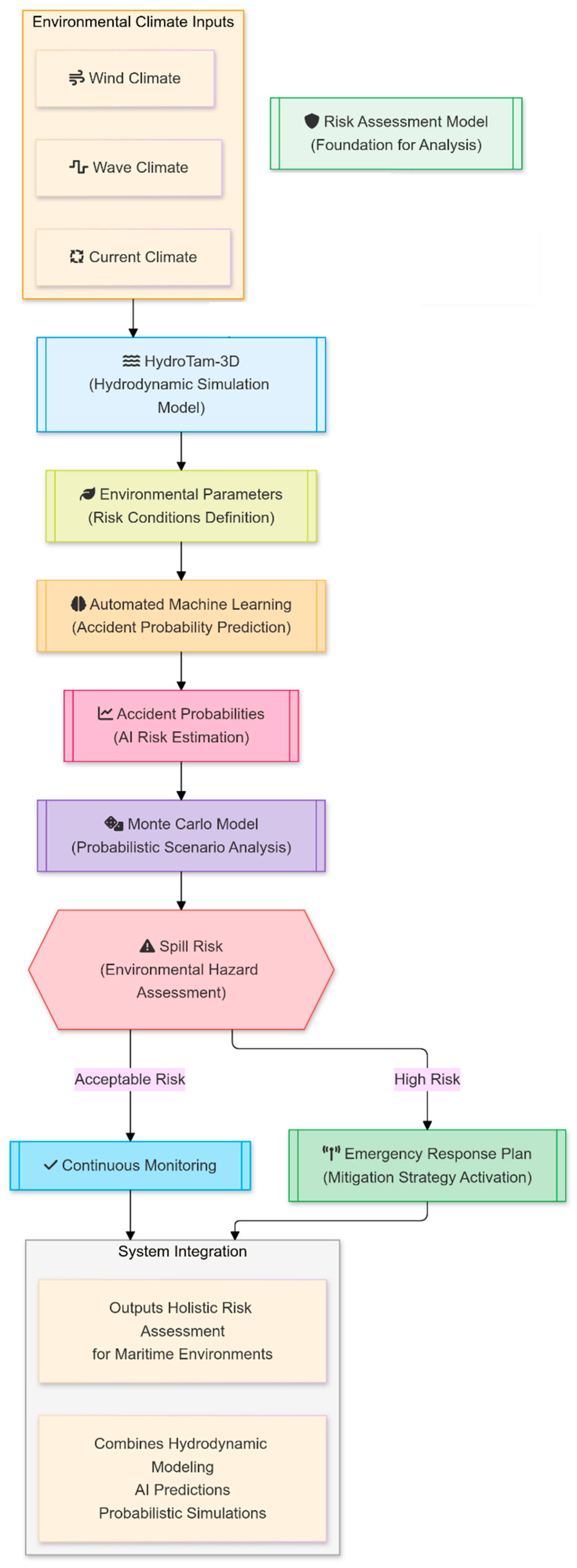
2. The Hybrid Maritime Risk Assessment (HMRA) Model
2.1. AML Sub-Models
- Division of the Dataset
- 2.
- Training Models
- 3.
- Multi-Classification Machine Learning
- 4.
- Breaking point
- 5.
- Testing and Evaluation
- 6.
- Cross-Validation
2.2. DL Sub-Models
2.2.1. The CNN-DL Model
2.2.2. The MLP-DL Model
2.2.3. The TensorFlow CNN-DL Model
2.2.4. The TensorFlow LSTM-DL Model
2.2.5. The TensorFlow MLP-DL Model
2.3. MCS Sub-Model
2.4. Wind Climate Model
2.5. Wave Climate Model
2.6. Current Climate Model
2.7. Pollutant Transport Model
3. Application of the Hybrid Model
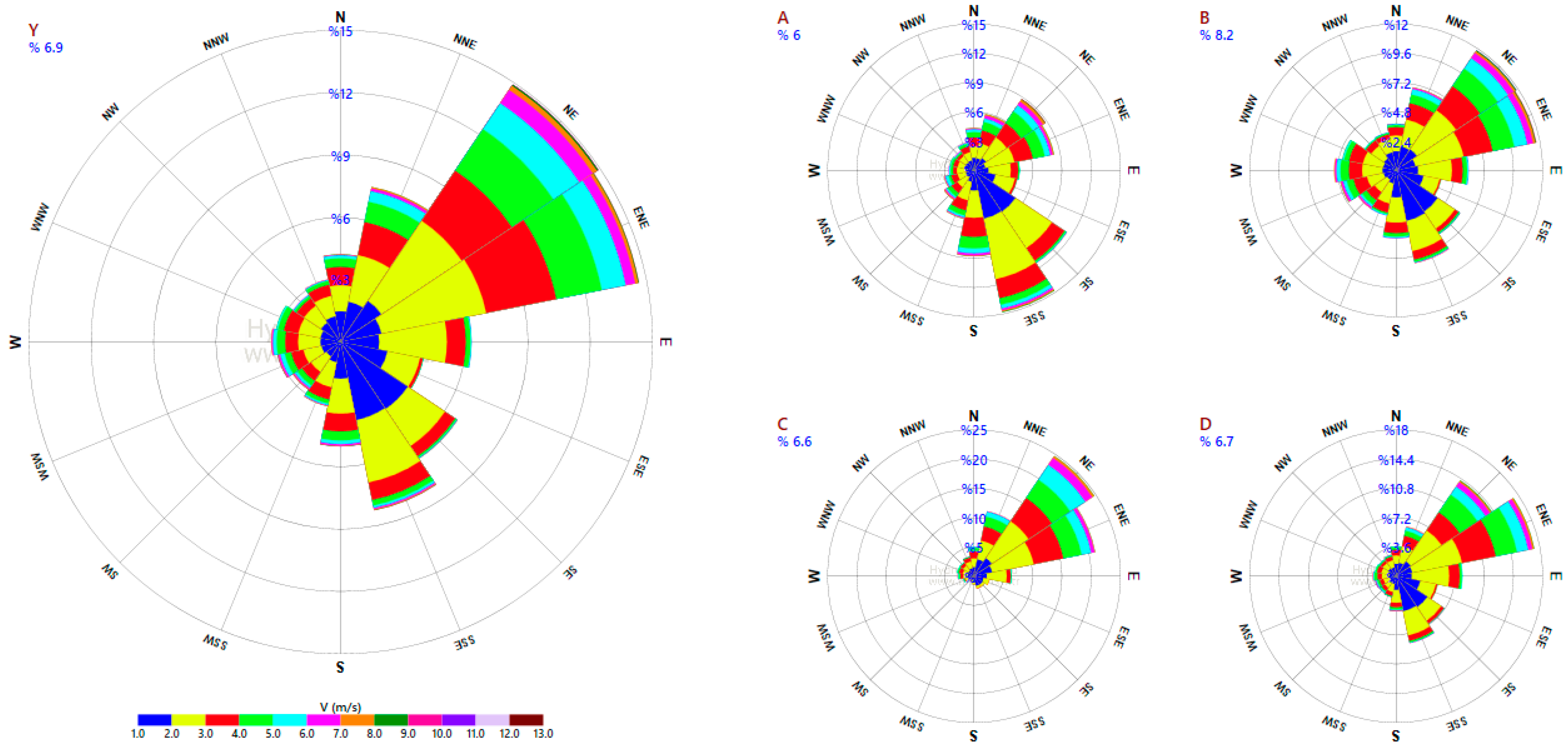
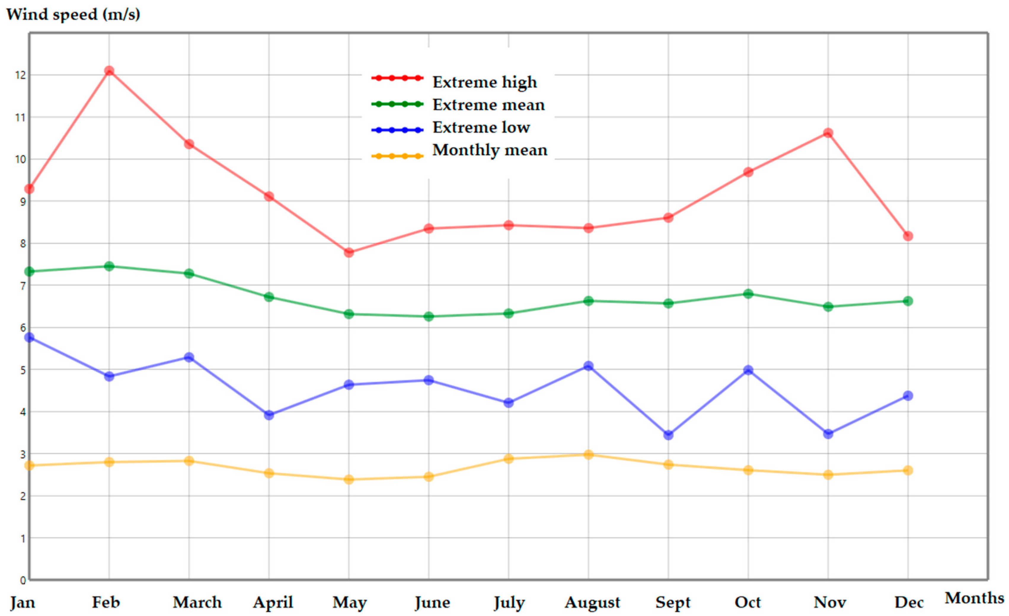
3.1. Wind Climate
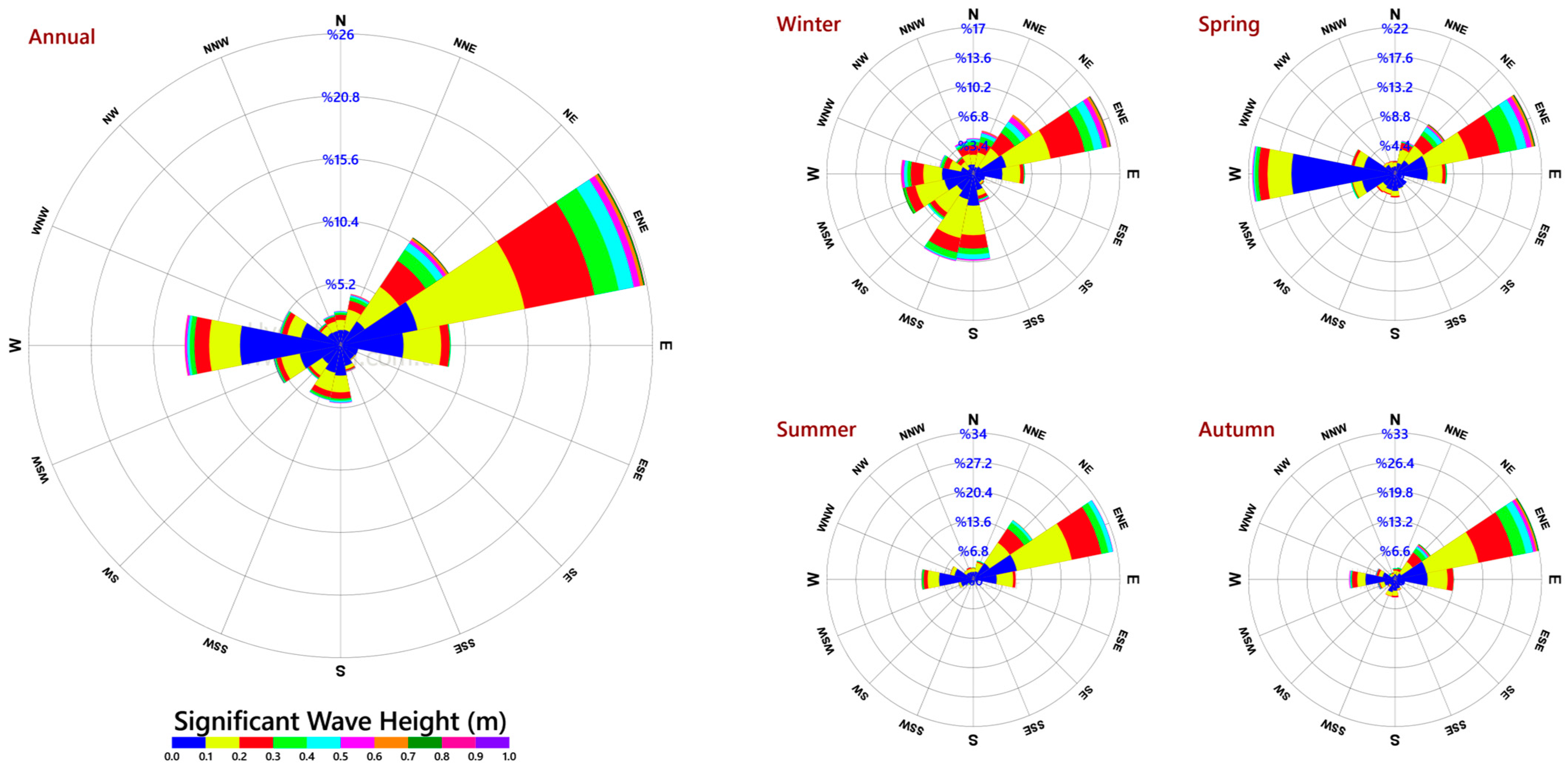
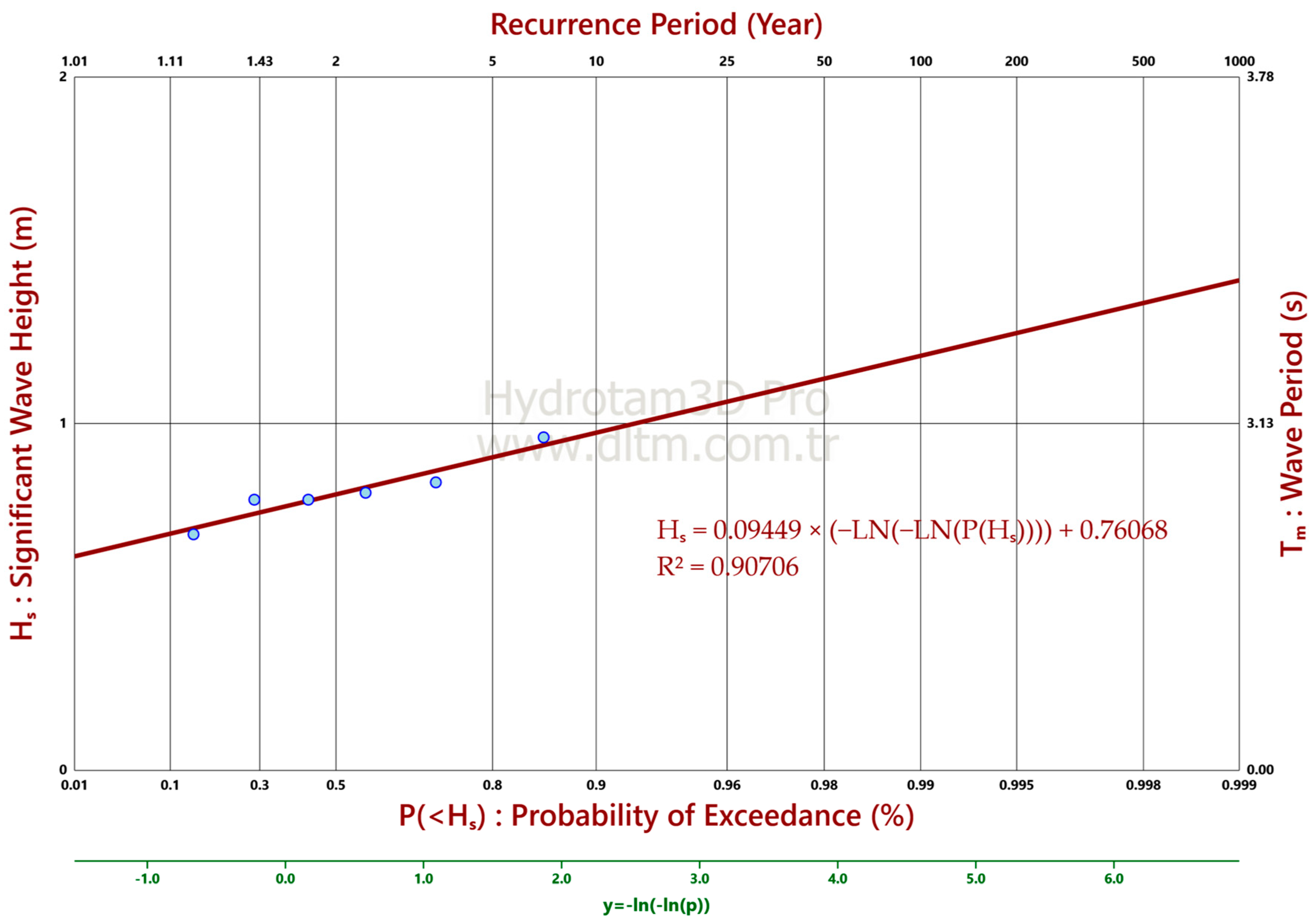
3.2. Wave Climate
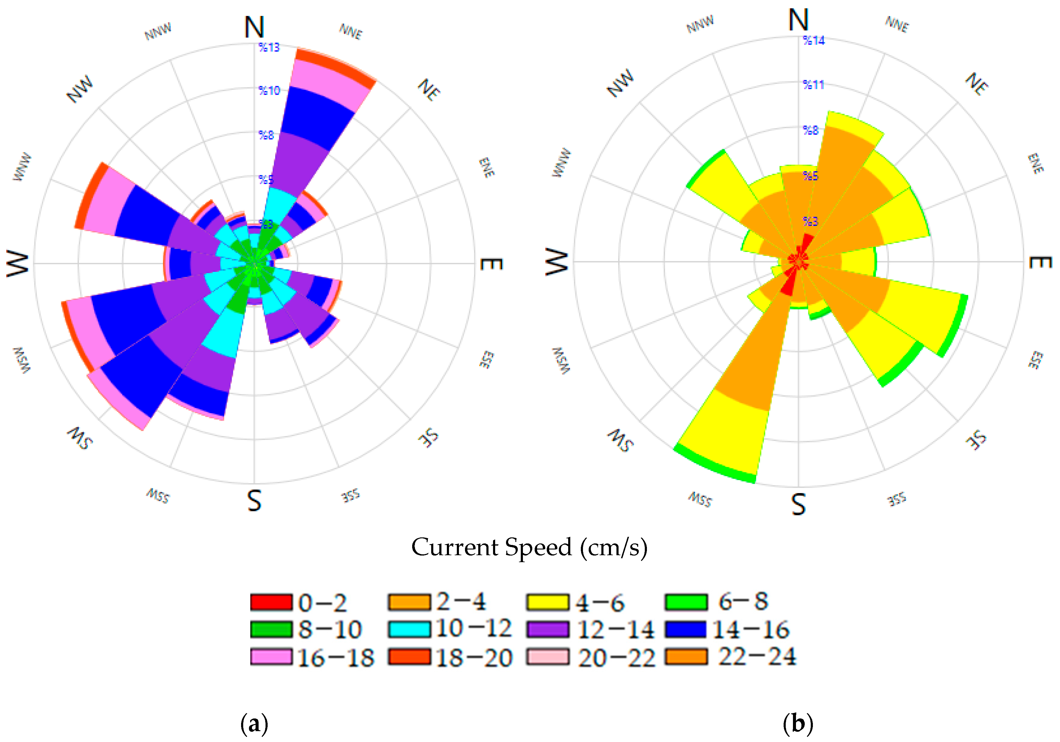
3.3. Current Climate
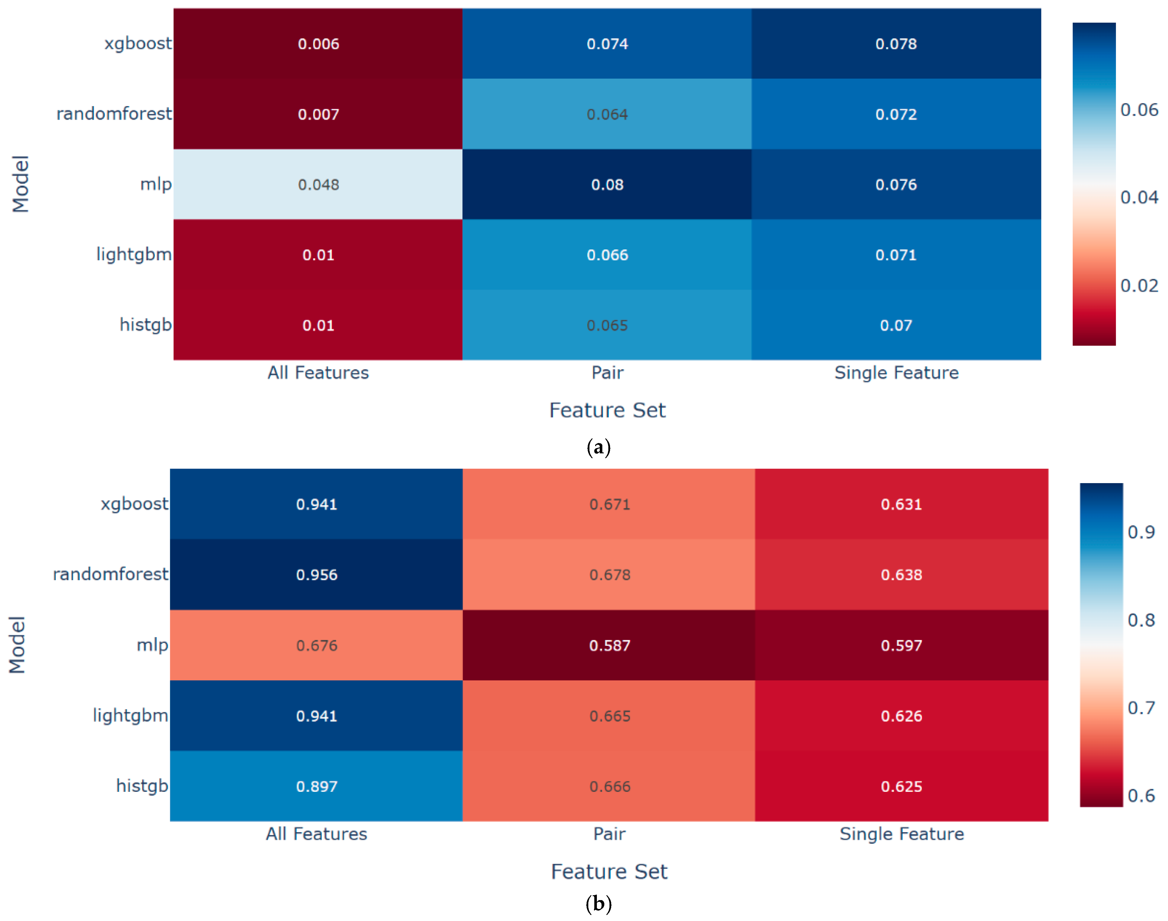
3.4. The AML and DL Sub-Models
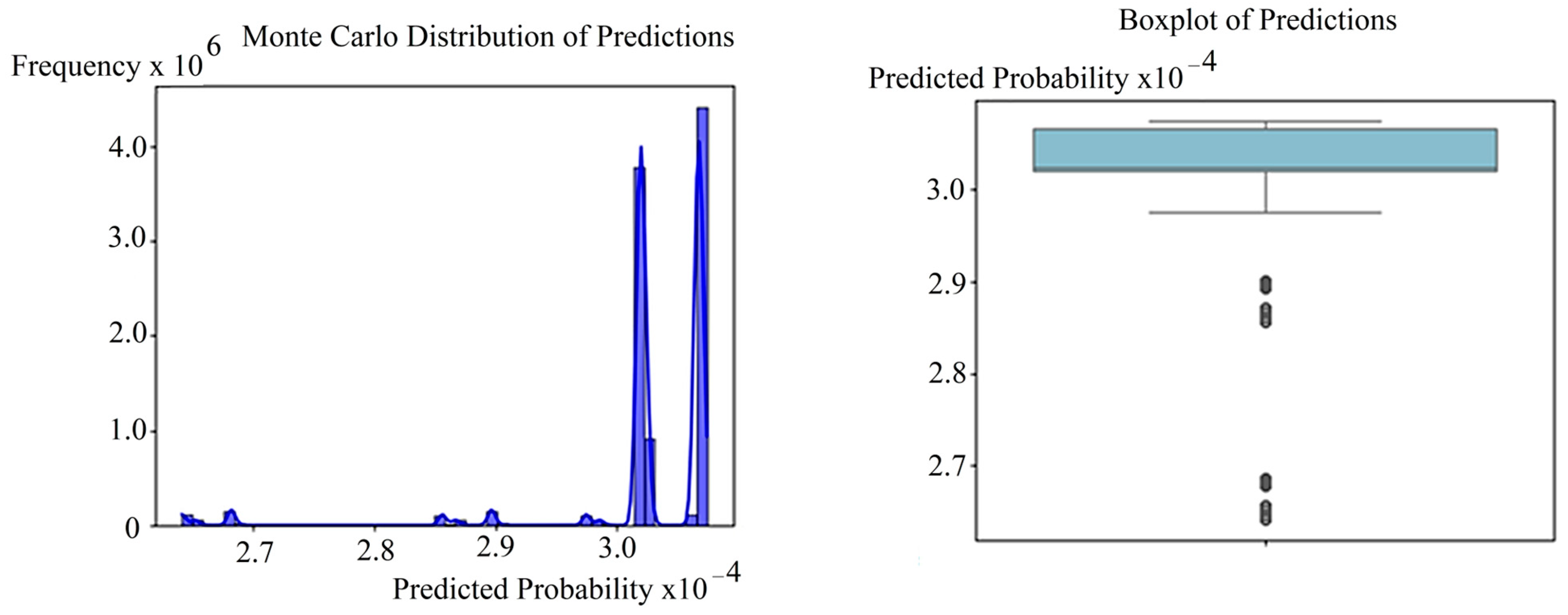
3.5. The MCS Sub-Model
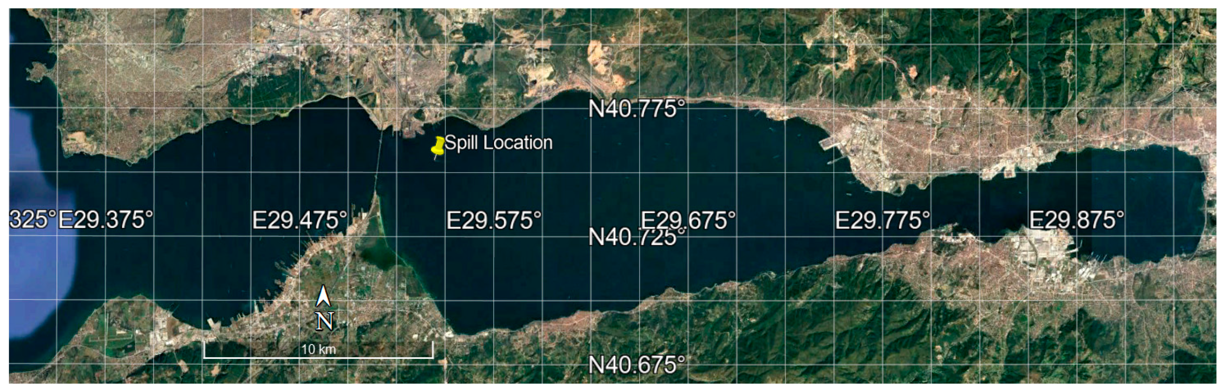
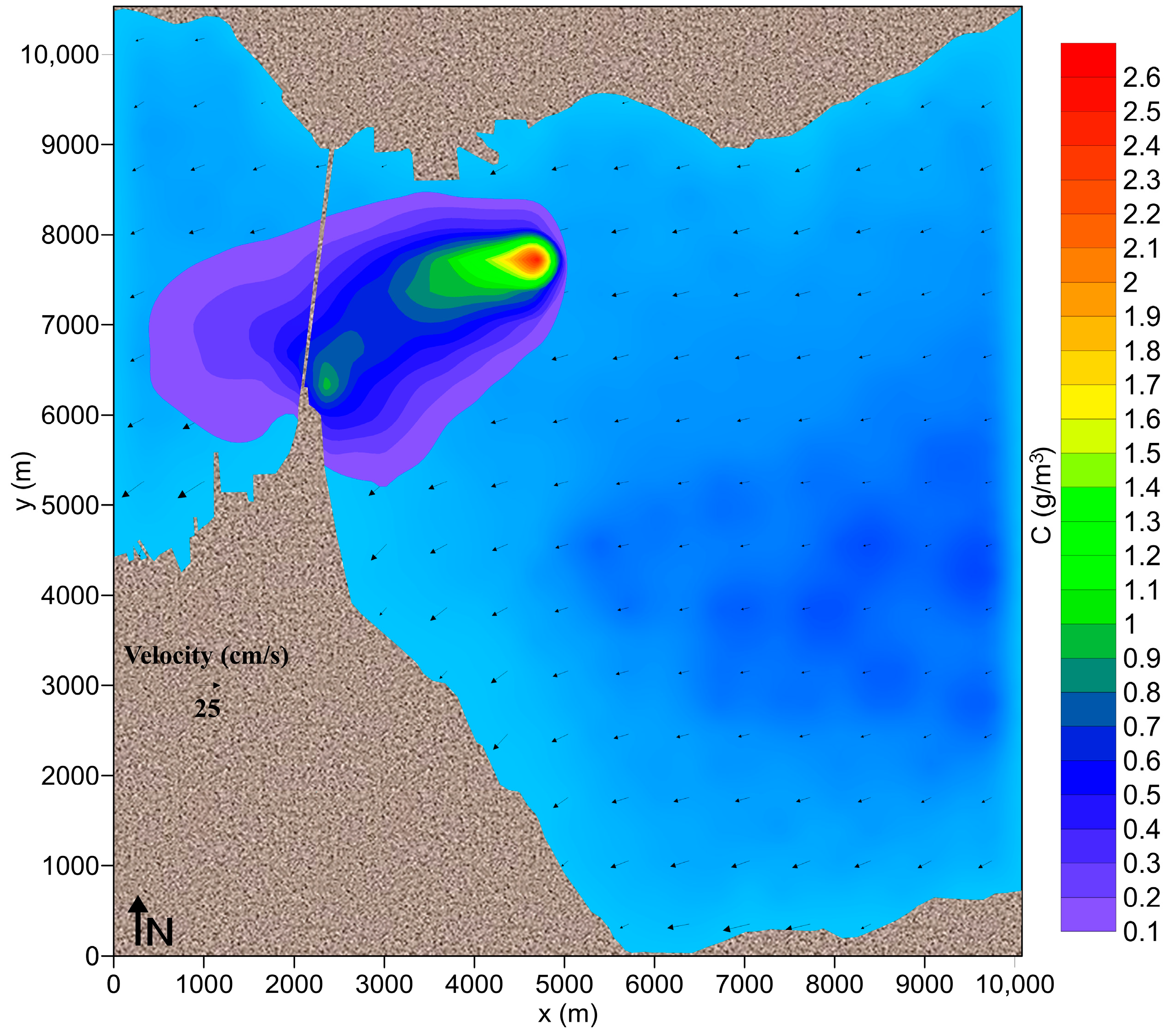
4. Hydrodynamic Transport Spill Simulation
- The evaporation rate of the spill is 19.6%,
- The density increase is 0.863 g/cm3,
- Viscosity is increased to 144 cSt,
- The spatial extent of the oil spill is 2 km.
5. Discussion of Results
6. Conclusions
7. Model Limitations
- Data Collection and Preparation
- Environmental Data: HYDROTAM 3D is calibrated using local environmental data, including meteorological conditions (wind, waves, currents).
- Vessel Traffic Data: Region-specific data on vessel types, traffic patterns, and operational behaviors, such as frequency, routes, and maneuvers, are obtained from maritime authorities.
- Accident Data: Accident records, including the types, causes, and outcomes of incidents, such as collisions, groundings, and oil spills, are acquired from maritime authorities.
- Calibration of the Hydrodynamic Model
- iii.
- Modeling Local Accident Types and Risk Factors
- Accident Categories: Accident types for the new region based on local maritime traffic and historical incident data are identified and categorized.
- Maneuvering and Vessel Behavior: Vessel-specific features, such as GT, LOA, and maneuvering difficulty, are determined using accident records to reflect regional ship types and behaviors.
- iv.
- Calibration of AML and DL models
- Feature Selection and Training: Environmental conditions, vessel characteristics, and operational factors are used to determine the most predictive features for the new region. AML models of LightGBM, XGBoost, Random Forest, and MLP are trained using region-specific accident data.
- Hyperparameter Tuning: Hyperparameter optimization and cross-validation are performed to fine-tune model performance for the target region.
- v.
- Calibration of MCS
- Local Spill Scenarios: MCS simulations of accident scenarios specific to the new region, including spill volumes, trajectories, and environmental impact based on regional maritime operations, are performed.
- Environmental Variability: Regional variability in factors such as wind speed, currents, and sea conditions, which affect oil spill behavior and environmental risk, is incorporated by the sensitivity analyses of MCS.
- vi.
- Performance Evaluation and Validation
8. Future Studies
Author Contributions
Funding
Data Availability Statement
Acknowledgments
Conflicts of Interest
Appendix A

| Ship Type | Accident Date | Time | Accident Location | Environmental Condition | GRT | LOA (m) | Port of Departure | Port of Arrival | Cargo Information | Crew | Severity |
|---|---|---|---|---|---|---|---|---|---|---|---|
| Bulk Cargo | 30 December 2024 | 15:20 | Tekirdağ | Wind and sea calm, good visibility | 14,909 | 159.9 | Dakar/Senegal | Aden/Yemen | Flour | 16 | Very Serious |
| Ferry | 2 March 2023 | 6:05 | 40°52′39″ N–37°34′04″ E | Wind NE 4 BF, Weather sunny, Wave 0.5–1.25 m, good visibility | 495 | 70 | Bandırma-Çelebi Port | Tekirdağ Ceyport | Passenger/Car | 6 | Serious |
| Tug | 31 August 2022 | 13:14 | Tuzla/İstanbul | Wind N to NE 7–12 knot calm sea, good visibility, weather clear | 103 | 18.7 | Özkaradeniz Shipyard | Özkaradeniz Shipyard | 4 | Very Serious | |
| Bulk Cargo | 31 August 2022 | 13:14 | Tuzla/İstanbul | Wind N to NE 7–12 knot calm sea, good visibility, weather clear | 5632 | 108.2 | İzmit | Tuzla | 12 | Very Serious | |
| Petrol Chemical Tanker | 28 August 2022 | 17:00 | Bandırma | Calm sea and wind, good weather, good visibility | 8391 | 135.6 | Reni/Ukraine | Bandırma | Crude sunflower oil | 15 | Very Serious |
| Chemical Tanker | 3 March 2022 | 12:15 | Bosphorus South Entrance Area C (40°56′6″ N–28°51′0″ E )/İstanbul | Wind from N to NW 4 to 6 BS, Wave height 1–1.5 m, weather rainy-cloudy, sea calm, good visibility | 2788 | 96 | Sisam/Greece | Kulevi/Georgia | 13 | Very Serious | |
| Agency Boat | 3 March 2022 | 12:15 | Bosphorus South Entrance Area C (40°56′6″ N–28°51′0″E)/İstanbul | Wind from N to NW 4 to 6 BS, Wave height 1–1.5 m, weather rainy-cloudy, sea 7 C, good visibility | 24.97 | 14.3 | Zeyport/İstanbul | Zeyport/İstanbul | 2 | Very Serious | |
| Bulk Cargo | 8 September 2021 | 14:10 | İzmit Belde Port/İzmit | Wind from E 4 BS, weather partly cloudy, the Sea is at 2 Beaufort scale, good visibility | 19,825 | 175.53 | Shanghai China | Poti/Georgia | Roll Sheet/Chipboard/Sheet Metal | 23 | Very Serious |
| Container | 17 June 2021 | 15:12 | Bosphorus Northern Exit/İstanbul | Breeze north, calm sea, good visibility, weather clear | 17,068 | 180.42 | Haydarpaşa | Constanta/Romania | 6840 MT containers | 17 | Very Serious |
| Fishing Boat | 17 June 2021 | 15:12 | Bosphorus Northern Exit/İstanbul | Breeze north, calm sea, good visibility, weather clear | 3.09 | 7.3 | Poyrazköy Port | Büyük Liman | 3 | Very Serious | |
| Bulk Cargo | 26 November 2019 | 19:15 | Karabiga | Wind S to SE 3–5 BF, calm sea, Rainy weather, good visibility | 784 | 54.9 | Marmara Island | Offshore of Şarköy/Tekirdağ | Concrete block | 6 | Very Serious |
| Bulk Cargo | 13 March 2019 | 17:40 | Marmara Island | Wind NE 4 BF, Weather cloudy, Wave 2–2.5 m, Good visibility | 994 | 76.15 | Marmara Island/Turkey | İzmit/Turkey | 1606 MT calcite | 7 | Very Serious |
| Bulk Cargo | 7 April 2018 | 15:33 | Bosphorus/İstanbul | Wind N to NE 4 BF, moderate sea, good visibility, overcast weather | 38,732 | 225 | Kavkaz Russia | Cidde Saudi Arabia | 20 | Serious | |
| Split Barge | 31 January 2018 | 4:30 | Safiport Derince/İzmit | Wind from N 12–19 km/h, Wave height 0.2–0.3m, good visibility | 376.31 | 48.5 | Dirt | 3 | Occupational Accident | ||
| Bulk Cargo | 10 January 2018 | 15:30 | Derince Port/İzmit | Calm sea and wind, cloudy weather, good visibility | 1249 | 79.3 | Elefsis/Greece | İzmit/Turkey | 11 | Occupational Accident | |
| Ferry | 7 December 2017 | 0:13 | Front of Port of Gestaş/Gelibolu | Wind SE direction 1–3 knot, sea calm, good visibility | 466 | 47.66 | Çardak/Çanakkale | Gelibolu/Çanakkale | Passenger/Car | 5 | Very Serious |
| Boat | 7 December 2017 | 0:13 | Front of Gestaş Port/Gelibolu | Wind SE direction 1–3 knot, sea calm, good visibility | 4–5m | 2 | Very Serious | ||||
| Bulk Cargo | 5 December 2017 | 15:06 | Marmara Ereğli/Tekirdağ | Wind from N 1–2 BS, weather clear, calm sea, good visibility | 31,538 | 190 | Kocaeli | Cristobal/Panama | 33,378 MT steel rebar | 20 | Very Serious |
| Bulk Cargo | 1 November 2017 | 3:52 | Şile/İstanbul | Wind from W to NW 4 to 5 BS, Wave height 1.5–2.5 m, weather partly cloudy, calm sea, good visibility | 1863 | 78.5 | Gemlik | Karadeniz Ereğli | 3150 MT tuff | 9 | Very Serious |
| LPG TANKER | 29 April 2017 | 16:30 | Habaş Platform/Yarımca | Wind East to SE 2–4 BF, Wave height 0.5–1 m, Good Visibility | 6529 | 112.16 | Temruk/Russia | Habaş Platform/İzmit | Air LPG mix | 24 | Very Serious |
| Agency Boat | 29 April 2017 | 16:30 | Habaş Platform/Yarımca | Wind East to SE 2–4 BF, Wave height 0.5–1 m, Good Visibility | 10.96 | 9.5 | 11 | Very Serious | |||
| Bulk Cargo | 14 May 2017 | 15:50 | Çelebi Bandırma Port/Sea of Marmara | Wind from NE 3 to 4 BS, clear weather, calm sea, good visibility | 1998 | 77 | Gemlik | Ambarlı | 96 TEU containers | 13 | Serious |
| Model | Hyperparameters | Feature List | CV MSE | CV R2 | Test MSE | Test RMSE | Test MAE | Test R2 | CV Accuracy | Test Accuracy | Test Precision | Test Recall | Test F1 | Test Balanced Accuracy | Test Log Loss |
|---|---|---|---|---|---|---|---|---|---|---|---|---|---|---|---|
| XgBoost | Objective: R2 error Random state: 42 Learning rate: 0.05 Max depth: 6 N estimators: 200 | Direction of daily Max Wind Maneuver Difficulty | 0.00638 | 0.893 | 0.00700 | 0.0837 | 0.0597 | 0.907 | 0.919 | 0.941 | 0.909 | 1.000 | 0.952 | 0.929 | 0.348 |
| XgBoost | Objective: R2 error Random state: 42 Learning rate: 0.05 Max depth: 6 N estimators: 200 | Monthly Average Wind Maneuver Difficulty | 0.00645 | 0.893 | 0.01612 | 0.1269 | 0.0726 | 0.785 | 0.896 | 0.882 | 0.833 | 1.000 | 0.909 | 0.857 | 0.364 |
| Random Forest | Random state: 42 | Direction of daily max wind Maneuver Difficulty | 0.00678 | 0.885 | 0.00696 | 0.0834 | 0.0601 | 0.907 | 0.926 | 0.941 | 0.909 | 1.000 | 0.952 | 0.929 | 0.347 |
| XgBoost | Objective: R2 error Random state: 42 | Sea Condition Maneuver Difficulty | 0.00684 | 0.888 | 0.01144 | 0.1070 | 0.0656 | 0.847 | 0.926 | 0.971 | 0.952 | 1.000 | 0.976 | 0.964 | 0.357 |
| Histgb | Random state: 42, Max iteration: 200, Max depth: 6 Learning rate: 0.05 Min samples leaf: 10 | Maneuver Difficulty Average Turn of Vessel | 0.00684 | 0.886 | 0.00835 | 0.0914 | 0.0579 | 0.889 | 0.926 | 0.941 | 0.909 | 1.000 | 0.952 | 0.929 | 0.348 |
| Random Forest | Random state: 42 | Maneuver Difficulty | 0.00720 | 0.877 | 0.00823 | 0.0907 | 0.0569 | 0.890 | 0.926 | 0.941 | 0.909 | 1.000 | 0.952 | 0.929 | 0.349 |
| Random Forest | Random state: 42 | Monthly Average Wind Average Current | 0.00724 | 0.881 | 0.01117 | 0.1057 | 0.0608 | 0.851 | 0.896 | 0.912 | 0.870 | 1.000 | 0.930 | 0.893 | 0.356 |
| Random Forest | Random state: 42 | Monthly Foggy Days, Direction of daily max wind, Average Current, Maneuver Difficulty, LOA | 0.00762 | 0.876 | 0.00678 | 0.0823 | 0.0554 | 0.910 | 0.911 | 0.941 | 0.909 | 1.000 | 0.952 | 0.929 | 0.342 |
| XgBoost | Objective: R2 error Random state: 42 | Monthly Foggy Days, Direction of daily max wind, Average Current, Maneuver Difficulty, LOA | 0.00827 | 0.865 | 0.00784 | 0.0885 | 0.0602 | 0.895 | 0.896 | 0.941 | 0.909 | 1.000 | 0.952 | 0.929 | 0.333 |
| Random Forest | Random state: 42 N estimators: 200 Max depth: 10 Min sample split: 5 Min samples leaf: 2 | Monthly Foggy Days Direction of daily max wind Average Current Maneuver Difficulty LOA | 0.00925 | 0.842 | 0.00726 | 0.0852 | 0.0569 | 0.903 | 0.896 | 0.941 | 0.909 | 1.000 | 0.952 | 0.929 | 0.347 |
| Histgb | Random state: 42 | Monthly Foggy Days Direction of daily max wind, Average Current Maneuver Difficulty LOA | 0.00963 | 0.837 | 0.01088 | 0.1043 | 0.0651 | 0.855 | 0.904 | 0.882 | 0.833 | 1.000 | 0.909 | 0.857 | 0.365 |
| Histgb | Random state: 42 Max iteration: 200 Learning rate: 0.05 Max depth: 6 Min samples leaf: 20 | Monthly Foggy Days Direction of daily max wind, Average Current Maneuver Difficulty LOA | 0.00977 | 0.835 | 0.01038 | 0.1019 | 0.0642 | 0.862 | 0.896 | 0.912 | 0.905 | 0.950 | 0.927 | 0.904 | 0.363 |
| LightGbm | Objective: Regression Random state: 42 Verbosity: −1 | Monthly Foggy Days Direction of daily max wind, Average Current Maneuver Difficulty LOA | 0.01215 | 0.785 | 0.01017 | 0.1009 | 0.0746 | 0.864 | 0.889 | 0.941 | 0.909 | 1.000 | 0.952 | 0.929 | 0.384 |
| LightGbm | Objective: Regression, Random state: 42, Verbosity: −1 Num leaves: 31, Learning rate: 0.05, Max depth: 6, Min samples: 20, Subsample: 0.8, Co-sample by tree: 0.8 | Monthly Foggy Days Direction of daily max wind, Average Current Maneuver Difficulty LOA | 0.01580 | 0.727 | 0.01499 | 0.1225 | 0.0979 | 0.800 | 0.881 | 0.941 | 0.909 | 1.000 | 0.952 | 0.929 | 0.413 |
| MLP | Random state: 42 Hidden layer sizes: 50 Max iteration: 500 | Monthly Foggy Days, Direction of daily max wind, Average Current Maneuver Difficulty LOA | 0.03775 | 0.381 | 0.04799 | 0.2191 | 0.1827 | 0.360 | 0.800 | 0.706 | 0.679 | 0.950 | 0.792 | 0.654 | 0.580 |
| MLP | Random state: 42 Hidden layers 100 Max iteration: 1000 Learning rate: Adaptive Early stopping: True | Monthly Foggy Days Direction of daily max wind Average Current Maneuver Difficulty LOA | 0.05964 | 0.033 | 0.01976 | 0.1406 | 0.0890 | 0.736 | 0.533 | 0.765 | 0.714 | 1.000 | 0.833 | 0.714 | 0.439 |
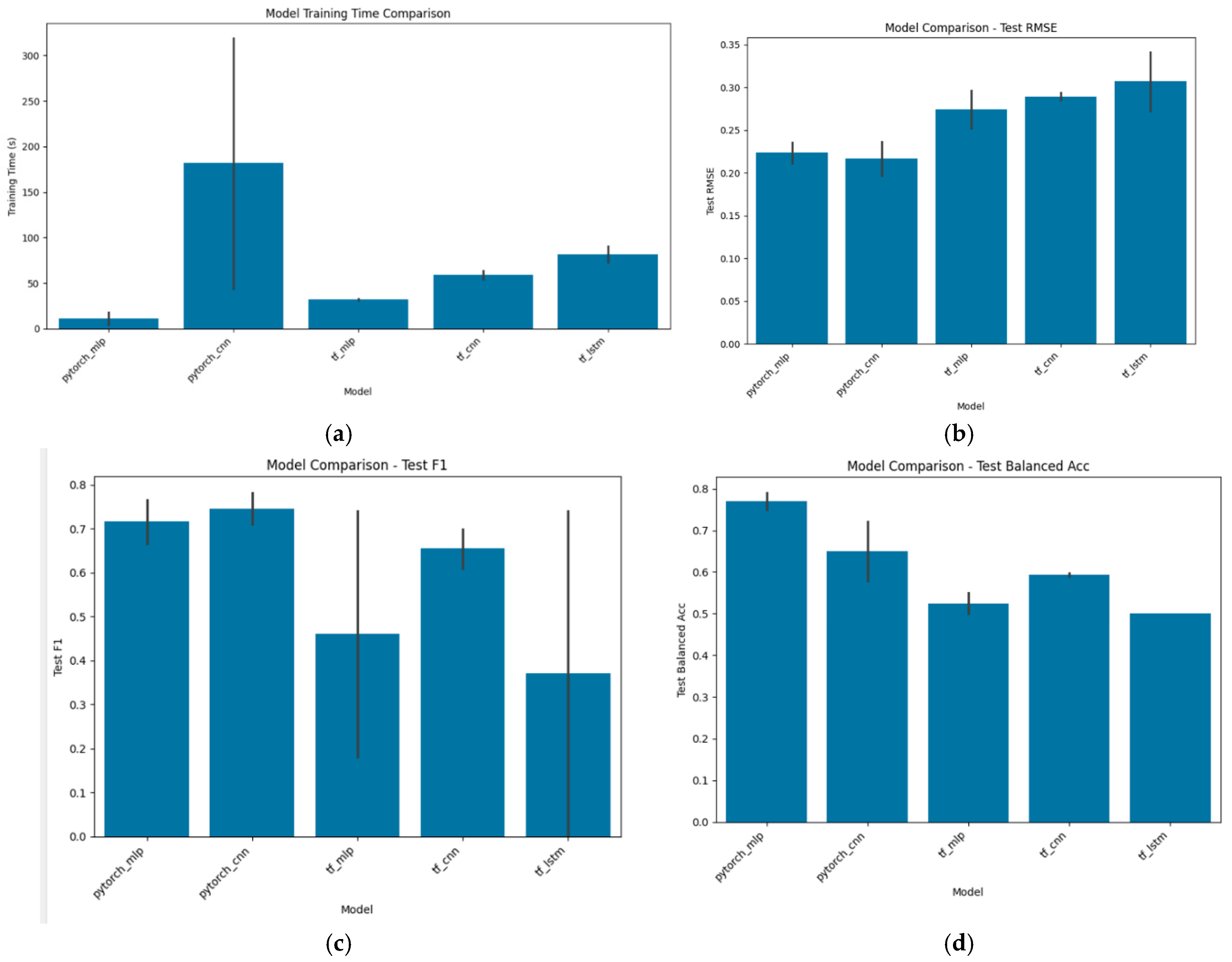
| Model | Training Time (s) | CV MSE (Mean) | CV MSE (std) | Test MSE | Test RMSE | Test MAE | CV Accuracy (Mean) | CV Balanced Acc (Mean) | CV Log Loss (Mean) | Test Accuracy | Test Precision | Test Recall | Test F1 | Test Balanced Acc |
|---|---|---|---|---|---|---|---|---|---|---|---|---|---|---|
| CNN Tuned | 43.9682 | 0.0320 | 0.0101 | 0.4882 | 0.0559 | 0.2365 | 0.1995 | 0.2537 | 0.7630 | 0.7835 | 0.5258 | 0.7353 | 0.7619 | 0.8000 |
| CNN Baseline | 319.3604 | 0.0382 | 0.0114 | 0.3787 | 0.0388 | 0.1971 | 0.1528 | 0.4816 | 0.7111 | 0.6938 | 0.5830 | 0.6176 | 0.6400 | 0.8000 |
| TF LSTM Tuned | 90.7243 | 0.0646 | 0.0108 | −0.0271 | 0.0746 | 0.2731 | 0.2407 | 0.0048 | 0.6000 | 0.4983 | 0.6764 | 0.5882 | 0.5882 | 1.0000 |
| TF CNN Tuned | 63.8258 | 0.0719 | 0.0331 | −0.0970 | 0.0812 | 0.2850 | 0.2473 | −0.0843 | 0.5407 | 0.5706 | 0.6725 | 0.6176 | 0.6522 | 0.7500 |
| MLP Tuned | 17.8127 | 0.0820 | 0.0560 | −0.4342 | 0.0447 | 0.2115 | 0.1820 | 0.4032 | 0.7037 | 0.7148 | 0.6027 | 0.7647 | 0.9286 | 0.6500 |
| TF CNN Baseline | 54.5599 | 0.0970 | 0.0701 | −0.4581 | 0.0863 | 0.2938 | 0.2413 | −0.1520 | 0.5333 | 0.6012 | 0.7529 | 0.5882 | 0.6875 | 0.5500 |
| TF MLP Baseline | 31.0620 | 0.1010 | 0.0553 | −0.7347 | 0.0876 | 0.2960 | 0.2479 | −0.1695 | 0.5556 | 0.5365 | 0.7792 | 0.4706 | 1.0000 | 0.1000 |
| TF MLP Tuned | 32.6604 | 0.1406 | 0.1089 | −1.0670 | 0.0634 | 0.2519 | 0.2294 | 0.1533 | 0.4963 | 0.5387 | 0.9898 | 0.5882 | 0.5882 | 1.0000 |
| MLP Baseline | 4.3379 | 0.1602 | 0.1500 | −1.9381 | 0.0555 | 0.2357 | 0.2126 | 0.2587 | 0.6963 | 0.6867 | 1.5766 | 0.7059 | 1.0000 | 0.5000 |
References
- Main Search and Rescue Coordination Center. Accident and Events Statistics, 2016–2024; Main Search and Rescue Coordination Center: Ankara, Turkey, 2024. Available online: https://ulasimemniyeti.uab.gov.tr/uploads/pages/istatistikler/deniz-1.pdf (accessed on 17 April 2025).
- UNCTAD. UNCTAD/RMT/2023 Review of Maritime Transport; United Nations Conference on Trade and Development: New York, NY, USA, 2023; ISBN 978-92-1-358456-9. Available online: https://unctad.org/publication/review-maritime-transport-2023 (accessed on 3 February 2024).
- OECD. Globalisation, Transport and the Environment; Organisation for Economic Cooperation and Development OECD: Paris, France, 2010; ISBN 9789264079199. [Google Scholar]
- Usluer, H.B.; Alkan, G.; Turan, O. A Ship Maneuvers Could be Predicted in the Turkish Straits by Marine Science Effects? Int. J. Environ. Geoinformatics 2022, 9, 95–101. [Google Scholar] [CrossRef]
- Yildiz, S.; Uğurlu, Ö.; Wang, J.; Loughney, S. Application of the HFACS-PV approach for identification of human and organizational factors (HOFs) influencing marine accidents. Reliab. Eng. Syst. Saf. 2021, 208, 107395. [Google Scholar] [CrossRef]
- IPIECA. Oil Spill Preparedness and Response: An Introduction Guidance Document for the Oil and Gas Industry; International Petroleum Industry Environmental Conservation Association: London, UK, 2019; Available online: https://www.ipieca.org/work/marine-spill-preparedness-and-response (accessed on 4 February 2024).
- IMO. Guide to Maritime Security & The ISPS Code, International Maritime Organization; IMO: London, UK, 2021; ISBN 978-9280117400. Available online: https://www.imo.org/en/OurWork/Security/Pages/SOLAS-XI-2%20ISPS%20Code.aspx (accessed on 3 February 2024).
- Kayıran, B.; Yazır, D.; Aslan, B. Data-driven Bayesian network approach to maritime accidents involved by dry bulk carriers in Turkish search and rescue areas. Reg. Stud. Mar. Sci. 2023, 67, 103193. [Google Scholar] [CrossRef]
- Arslanoglu, B.; Elidolu, G.; Uyanık, T. Application of Machine Learning Methods for Prediction of Seafarer Safety Perception. Int. J. Marit. Eng. 2023, 164, 269–282. [Google Scholar] [CrossRef]
- Korçak, M.; Balas, C.E. Reducing the probability for the collision of ships by changing the passage schedule in Istanbul Strait. Int. J. Disaster Risk Reduct. 2020, 48, 101593. [Google Scholar] [CrossRef]
- Sakar, C.; Toz, A.C.; Buber, M.; Koseoglu, B. Risk Analysis of Grounding Accidents by Mapping a Fault Tree Into a Bayesian Network. Appl. Ocean Res. 2021, 113, 102764. [Google Scholar] [CrossRef]
- Galieriková, A.; Dávid, A.; Materna, M.; Mako, P. Study of maritime accidents with hazardous substances involved: Comparison of HNS and oil behaviours in marine environment. Transp. Res. Procedia 2021, 55, 1050–1064. [Google Scholar] [CrossRef]
- Ekici, C.V.; Öztürk, Ü.; Şenol, Y.E. A data-driven Ship Risk Profile model for Turkish Straits (TS-SRP) using Machine Learning. Ocean Eng. 2024, 311, 119002. [Google Scholar] [CrossRef]
- IMO. Convention on the International Regulations for Preventing Collisions at Sea (COLREG); IMO: London, UK, 2016; Available online: https://www.imo.org/en/About/Conventions/Pages/COLREG.aspx (accessed on 4 February 2024).
- Saçu, Ş.; Şen, O.; Erdik, T. A stochastic assessment for oil contamination probability: A case study of the Bosphorus. Ocean Eng. 2021, 231, 109064. [Google Scholar] [CrossRef]
- Dimitrakiev, D.; Milev, D.; Gunes, E. The Risk Analysis of Chemical Tankers Passing Through the Turkish Straits between 2010–2022. Strateg. Policy Sci. Educ.-Strateg. Na Obraz. Nauchnata Polit. 2023, 31, 45–55. [Google Scholar] [CrossRef]
- Lee, D.; Namgung, H.; Yoo, S.-L. Development of a Risk Assessment System for Navigational Obstacles Considering Collision and Pollution Risks. Appl. Sci. 2025, 15, 2325. [Google Scholar] [CrossRef]
- Uyanık, T.; Karatuğ, Ç.; Arslanoğlu, Y. Machine learning based visibility estimation to ensure safer navigation in strait of Istanbul. Appl. Ocean Res. 2021, 112, 102693. [Google Scholar] [CrossRef]
- Rawson, A.; Brito, M.; Sabeur, Z.; Tran-Thanh, L. A machine learning approach for monitoring ship safety in extreme weather events. Saf. Sci. 2021, 141, 105336. [Google Scholar] [CrossRef]
- Merrick, J.R.W.; Dorsey, C.A.; Wang, B.; Grabowski, M.; Harrald, J.R. Measuring Prediction Accuracy in a Maritime Accident Warning System. Prod. Oper. Manag. 2022, 31, 819–827. [Google Scholar] [CrossRef]
- Rawson, A.; Brito, M.; Sabeur, Z. Spatial Modeling of Maritime Risk Using Machine Learning. Risk Anal. 2022, 42, 2291–2311. [Google Scholar] [CrossRef]
- Liu, K.; Yu, Q.; Yuan, Z.; Yang, Z.; Shu, Y. A systematic analysis for maritime accidents causation in Chinese coastal waters using machine learning approaches. Ocean. Coast. Manag. 2021, 213, 105859. [Google Scholar] [CrossRef]
- Feng, Y.; Wang, X.; Chen, Q.; Yang, Z.; Wang, J.; Li, H.; Xia, G.; Liu, Z. Prediction of the severity of marine accidents using improved machine learning. Transp. Res. E Logist. Transp. Rev. 2024, 188, 103647. [Google Scholar] [CrossRef]
- Brandt, P.; Munim, Z.H.; Chaal, M.; Kang, H.-S. Maritime accident risk prediction integrating weather data using machine learning. Transp. Res. D Transp. Environ. 2024, 136, 104388. [Google Scholar] [CrossRef]
- Munim, Z.H.; Sørli, M.A.; Kim, H.; Alon, I. Predicting maritime accident risk using Automated Machine Learning. Reliab. Eng. Syst. Saf. 2024, 248, 110148. [Google Scholar] [CrossRef]
- Madsen, P.M.; Dillon, R.L.; Morris, E.T. Using near misses, artificial intelligence, and machine learning to predict maritime incidents: A U.S. Coast Guard case study. Risk Anal. 2024, 45, 830–845. [Google Scholar] [CrossRef]
- Yuzui, T.; Kaneko, F. Toward a hybrid approach for the risk analysis of maritime autonomous surface ships: A systematic review. J. Mar. Sci. Technol. 2025, 30, 153–176. [Google Scholar] [CrossRef]
- Ugurlu, H.; Cicek, I. Analysis and assessment of ship collision accidents using Fault Tree and Multiple Correspondence Analysis. Ocean Eng. 2022, 245, 110514. [Google Scholar] [CrossRef]
- Adland, R.; Jia, H.; Lode, T.; Skontorp, J. The value of meteorological data in marine risk assessment. Reliab. Eng. Syst. Saf. 2021, 209, 107480. [Google Scholar] [CrossRef]
- Yang, Y.; Liu, Y.; Li, G.; Zhang, Z.; Liu, Y. Harnessing the power of Machine learning for AIS Data-Driven maritime Research: A comprehensive review. Transp. Res. E Logist. Transp. Rev. 2024, 183, 103426. [Google Scholar] [CrossRef]
- Korupoju, A.K.; Kapadia, V.; Vilwathilakam, A.S.; Samanta, A. Ship Collision Risk Evaluation using AIS and weather data through fuzzy logic and deep learning. Ocean Eng. 2025, 318, 120116. [Google Scholar] [CrossRef]
- Dağkıran, B.; Bolat, P. Weighting the factors affecting safety of navigation: A case study for the Gulf of İzmit, Türkiye. Marit. Technol. Res. 2024, 7, 274135. [Google Scholar] [CrossRef]
- Altalhan, M.; Algarni, A.; Turki-Hadj Alouane, M. Imbalanced Data Problem in Machine Learning: A Review. IEEE Access 2025, 13, 13686–13699. [Google Scholar] [CrossRef]
- Xiao, Y.; Jin, M.; Qi, G.; Shi, W.; Li, K.X.; Du, X. Interpreting the influential factors in ship detention using a novel random forest algorithm considering dataset imbalance and uncertainty. Eng. Appl. Artif. Intell. 2024, 133, 108369. [Google Scholar] [CrossRef]
- Painsky, A.; Wornell, G. On the Universality of the Logistic Loss Function. In Proceedings of the 2018 IEEE International Symposium on Information Theory (ISIT), Vail, CO, USA, 17–22 June 2018; pp. 936–940, ISBN 978-1-5386-4781-3. [Google Scholar] [CrossRef]
- Tian, Y.; Meng, H.; Yuan, F. FREGNet: Ship Recognition Based on Feature Representation Enhancement and GCN Combiner in Complex Environment. IEEE Trans. Intell. Transp. Syst. 2024, 25, 15641–15653. [Google Scholar] [CrossRef]
- Kamal, B.; Çakır, E. Data-driven Bayes approach on marine accidents occurring in Istanbul strait. Appl. Ocean Res. 2022, 123, 103180. [Google Scholar] [CrossRef]
- Wang, M.; Wang, Y.; Ding, J.; Yu, W. Interaction aware and multi-modal distribution for ship trajectory prediction with spatio-temporal crisscross hybrid network. Reliab. Eng. Syst. Saf. 2024, 252, 110463. [Google Scholar] [CrossRef]
- Bologna, G. A Rule Extraction Technique Applied to Ensembles of Neural Networks, Random Forests, and Gradient-Boosted Trees. Algorithms 2021, 14, 339. [Google Scholar] [CrossRef]
- Balas, L.; Özhan, E. A Baroclinic Three Dimensional Numerical Model Applied to Coastal Lagoons. Comput. Sci. —ICCS 2003 2003, 2658, 205–212. [Google Scholar] [CrossRef]
- HYDROTAM-3D. HYDROTAM-3D, Three Dimensional Hydrodynamic Transport and Water Quality Model. 2025. Available online: http://www.hydrotam.com/ (accessed on 3 May 2023).
- Balas, L.; Inan, A.; Genc Numanoglu Asli. Modelling of Dilution of Thermal Discharges in Enclosed Coastal Waters. Res. J. Chem. Env. 2013, 17, 82–89. [Google Scholar]
- Genc Numanoğlu, A.; Inan, A.; Yilmaz, N.; Balas, L. Modeling of Erosion at Goksu Coasts. J. Coast. Res. 2013, 65, 2155–2160. [Google Scholar] [CrossRef]
- ECMWF. IFS Documentation CY41R2—Part III: Dynamics and Numerical Procedures. In IFS Documentation CY41R2; ECMWF: Reading, UK, 2016. [Google Scholar] [CrossRef]
- Uğurlu, A.; Balas, E.A.; Balas, C.E.; Akbaş, S.O. Unleashing the Potential of a Hybrid 3D Hydrodynamic Monte Carlo Risk Model for Maritime Structures’ Design in the Imminent Climate Change Era. J. Mar. Sci. Eng. 2024, 12, 931. [Google Scholar] [CrossRef]
- Balas, E.A. A hybrid Monte Carlo simulation risk model for oil exploration projects. Mar. Pollut. Bull. 2023, 194, 115270. [Google Scholar] [CrossRef]
- Durap, A.; Balas, C.E.; Çokgör, Ş.; Balas, E.A. An Integrated Bayesian Risk Model for Coastal Flow Slides Using 3-D Hydrodynamic Transport and Monte Carlo Simulation. J. Mar. Sci. Eng. 2023, 11, 943. [Google Scholar] [CrossRef]
- Ülker, D.; Burak, S.; Balas, L.; Çağlar, N. Mathematical modelling of oil spill weathering processes for contingency planning in Izmit Bay. Reg. Stud. Mar. Sci. 2022, 50, 102155. [Google Scholar] [CrossRef]
- General Directorate of Coastal Safety. General Directorate of Coastal Safety. Vessel Traffic Service of İzmit Bay. Available online: https://www.kiyiemniyeti.gov.tr/gemi_trafik_bilgi_sistemleri (accessed on 17 December 2024).
- Board of Transportation Safety. Board of Transportation Safety. Marine Accident Investigation Reports. Available online: https://ulasimemniyeti.uab.gov.tr/deniz (accessed on 17 February 2025).
- AASHTO. Guide Specifications and Commentary for Vessel Collision Design of Highway Bridges with Interim Revisions; AASHTO: Washington, DC, USA, 2009; Available online: https://store.transportation.org/Item/PublicationDetail?ID=1740 (accessed on 3 February 2024)ISBN 978-1-56051-495-4.
- Küçükosmanoğlu, A.; Arlı Küçükosmanoğlu, Ö. Estimation of Vessel Passage Through Bosphorus. Int. J. Eng. Appl. Sci. 2021, 13, 56–70. [Google Scholar] [CrossRef]
- Küçükosmanoğlu, A. Maritime Accidents Forecast Model for Bosphorus. Ph.D. Thesis, Middle East Technical University, Ankara, Turkey, 2012. [Google Scholar]
- Mazen, F.; Mazen, A. Airbus Ship Classification, Detection and Segmentation using Cutting-Edge Deep Learning Techniques. Fayoum Univ. J. Eng. 2025, 8, 68–78. [Google Scholar] [CrossRef]
- El Mekkaoui, S.; Benabbou, L.; Caron, S.; Berrado, A. Deep Learning-Based Ship Speed Prediction for Intelligent Maritime Traffic Management. J. Mar. Sci. Eng. 2023, 11, 191. [Google Scholar] [CrossRef]
- Zhang, X.; Lim, H.; Fu, X.; Wang, K.; Xiao, Z.; Qin, Z. Maritime-Context Text Identification for Connecting Artificial Intelligence (AI) Models. In Proceedings of the 2024 IEEE Conference on Artificial Intelligence (CAI), Singapore, 25–27 June 2024; pp. 899–904, ISBN 979-8-3503-5409-6. [Google Scholar] [CrossRef]
- Li, Y.; Yu, Q.; Yang, Z. Vessel Trajectory Prediction for Enhanced Maritime Navigation Safety: A Novel Hybrid Methodology. J. Mar. Sci. Eng. 2024, 12, 1351. [Google Scholar] [CrossRef]
- Jiang, X.; Dai, Y.; Li, S.; Ma, R.; Du, T.; Zou, Y.; Zhang, P.; Zhang, Y.; Sun, P. Research on ship speed prediction based on time series imaging and deep convolutional network fusion method. Appl. Ocean Res. 2025, 154, 104384. [Google Scholar] [CrossRef]
- Turkish Chamber of Shipping. Maritime Sector Report; Turkish Chamber of Shipping: İstanbul, Turkey, 2025; Available online: https://www.denizticaretodasi.org.tr/en/publications/sectorreport (accessed on 11 March 2024).
- Ministry of Transportation and Infrastructure. Turkish Straits Ship Passage Statistics. Available online: https://denizcilikistatistikleri.uab.gov.tr/turk-bogazlari-gemi-gecis-istatistikleri (accessed on 3 May 2025).
- European Maritime Safety Agency. Annual Overview of Marine Casualties and Incidents 2024; European Maritime Safety Agency: Lisbon, Portugal, 2024. [Google Scholar]
- Australian Maritime Safety Authority. Australian Maritime Safety Authority, National Plan to Combat Pollution of the Sea by Oil and Other Noxious and Hazardous Substances Annual Reports; Australian Maritime Safety Authority: Canberra, Australia, 2020. [Google Scholar]
- Det Norske Veritas. Final Report Assessment of the Risk of Pollution from Marine Oil Spills in Australian Ports and Waters, Model of Offshore Oil Spill Risks, Appendix V—Offshore Oil Spill Risk Models; Det Norske Veritas: Sydney, Australia, 2011. [Google Scholar]
- Australian Maritime Safety Authority. Great Barrier Reef Pilotage Fatigue Risk Assessment [Electronic Resource]; Australian Maritime Safety Authority: Canberra, Australia, 2001. [Google Scholar]
- ITOPF Tanker Owners Pollution Federation. Oil Tanker Spill Statistics; ITOPF Tanker Owners Pollution Federation: London, UK, 2025; Available online: https://www.itopf.org/knowledge-resources/data-statistics/ (accessed on 4 February 2024).
- Sackeyfio, N. Oil Tanker Spill Statistics Figures; Creative Commons Attribution License permission granted on 16 April 2025; ITOPF: London, UK, 2025. [Google Scholar]
- Balas, E.A.; Genç, A.N.; Balas, C.E. Strategic Adaptation to Climate Change through Monte Carlo-Based Multi-Criteria Decision Model in Marine Spatial Planning. J. Coast. Res. 2024, 113, 169–174. [Google Scholar] [CrossRef]
- Balas, E.A.; Uğurlu, A.; Balas, C.E. A Hybrid Probabilistic Design Model of Riverine Jetties Incorporating Three-Dimensional Numerical Simulations of Transport Phenomena in the Context of Emerging Climate Change. J. Coast. Res. 2024, 113, 220–224. [Google Scholar] [CrossRef]
- Buyruk, T.; Balas, E.A.; Genç, A.N.; Balas, L. Exploring Renewable Energy on the Coastline of Türkiye: Wind and Wave Power Potential. J. Coast. Res. 2024, 113, 788–792. [Google Scholar] [CrossRef]
- Balas Egemen, A. Numerical Modelling of Microplastics Transport in Mersin Bay. Master’s Thesis, Middle East Technical University, Ankara, Turkey, 2023. [Google Scholar]
- Wamdi Group. The WAM Model—A Third Generation Ocean Wave Prediction Model. J. Phys. Ocean. 1988, 18, 1775–1810. [Google Scholar] [CrossRef]
- Eun Choi, J.; Won Shin, J.; Wan Shin, D. Vector SHAP Values for Machine Learning Time Series Forecasting. J. Forecast. 2025, 44, 635–645. [Google Scholar] [CrossRef]
- Shintani, A.; Taniguchi, N.; Nakayama, Y.; Tanaka, T.; Hamada, K. Development of marine accident probability prediction model for pleasure boats using ship accident database in central part of Seto Inland Sea. Ocean Eng. 2025, 322, 120460. [Google Scholar] [CrossRef]
- Kriuchkova, A.; Toloknova, V.; Drin, S. Predictive model for a product without history using LightGBM. Pricing model for a new product. Mohyla Math. J. 2024, 6, 6–13. [Google Scholar] [CrossRef]
- Mariano Trainiti, G.; Piscopo, V.; Cianelli, D.; Zambianchi, E. Modelling Oil Spill and Dispersion at Sea from a Double Hull Oil Tanker Following Collision Events. In Proceedings of the 2024 IEEE International Workshop on Metrology for the Sea; Learning to Measure Sea Health Parameters (MetroSea), Portorose, Slovenia, 14–16 October 2024; pp. 181–185, ISBN 979-8-3503-7900-6. [Google Scholar] [CrossRef]
- Zhu, G.; Xie, Z.; Xu, H.; Wang, N.; Zhang, L.; Mao, N.; Cheng, J. Oil Spill Environmental Risk Assessment and Mapping in Coastal China Using Automatic Identification System (AIS) Data. Sustainability 2022, 14, 5837. [Google Scholar] [CrossRef]
- Vidmar, P.; Perkovič, M. Update on Risk Criteria for Crude Oil Tanker Fleet. J. Mar. Sci. Eng. 2023, 11, 695. [Google Scholar] [CrossRef]
- Asu, I.; Lale, B. Numerical Modelling of Oil Spill. In Proceedings of the 5th IASME/WSEAS Int Conf on Water Resources, Hydraulics & Hydrology/ Proceedings of the 4th IASME/WSEAS Int Conf on Geology and Seismology 2010, Cambridge, UK, 23–25 February 2010; pp. 62–73. [Google Scholar]
- Republic of Turkey Energy Market Regulatory Authority. Oil Market Industry Report of Türkiye; Annual Report; Republic of Turkey Energy Market Regulatory Authority: Ankara, Turkey, 2024. Available online: https://www.epdk.gov.tr/Detay/Icerik/2-14417/2024-yili-subat-ayi-petrol-piyasasi-sektor-raporu (accessed on 26 April 2025).
- Ülker, D. GIS-Based Modelling for Advection and Diffusion of Oil Pollution in Coastal Waters. PhD Thesis, İstanbul University, İstanbul, Turkey, 2022. [Google Scholar]
- Boranbayeva, L.; Boiko, G.; Sharifullin, A.; Lubchenko, N.; Sarmurzina, R.; Kozhamzharova, A.; Mombekov, S. Analysis of the Processes of Paraffin Deposition of Oil from the Kumkol Group of Fields in Kazakhstan. Processes 2024, 12, 1052. [Google Scholar] [CrossRef]
- Shrestha, A.; Mahmood, A. Review of Deep Learning Algorithms and Architectures. IEEE Access 2019, 7, 53040–53065. [Google Scholar] [CrossRef]
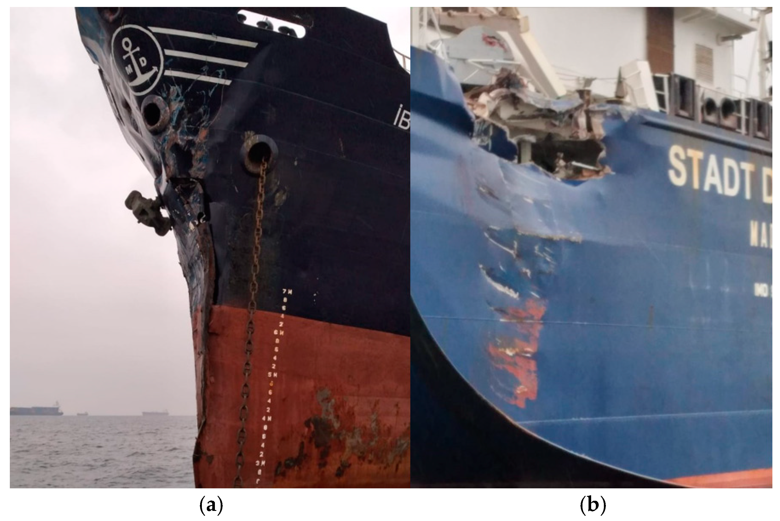
- Haber Global National Newspaper; İhlas News Agency. Two Dry Cargo Ships Collided in the Gulf of Izmit. Habertakvimi.com. 2020. Available online: https://haberglobal.com.tr/gundem/izmit-korfezi-nde-iki-kuru-yuk-gemisi-carpisti-33455 (accessed on 17 April 2025).
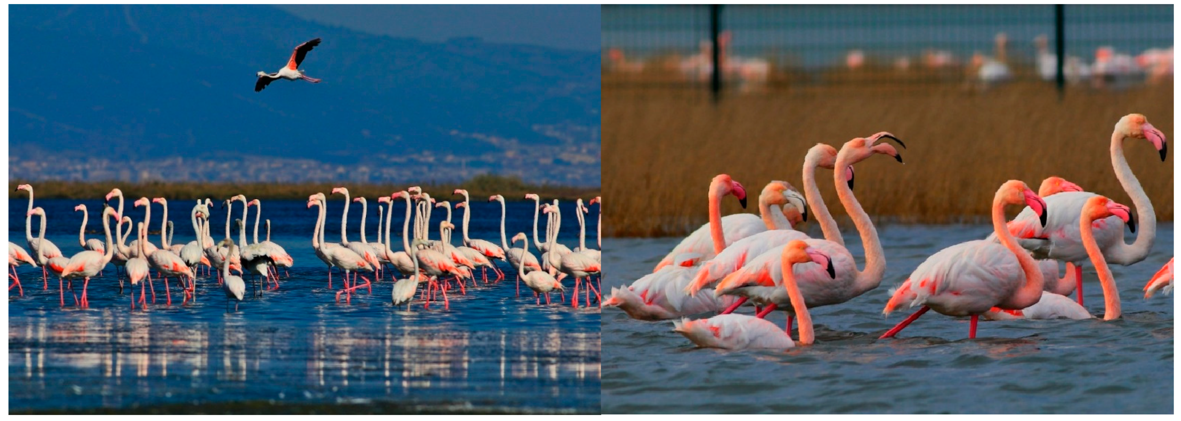
- Bülbül, F. Unpublished Nature Photographs; Altınordu, Türkiye, 2025. [Google Scholar]
- Daily Sabah. Turkish Lagoon Gives Shelter to Flamingos Fleeing Drought. Editorial Daily Sabah. 2022. Available online: https://www.dailysabah.com/turkey/turkish-lagoon-gives-shelter-to-flamingosfleeing-drought/news (accessed on 12 March 2025).
- Hisli, O.; Balkıs, H.; Mülayim, A. Macrobenthic Invertebrates of the Hersek Lagoon (Marmara Sea, Turkey) under Pollution Pressure. Acta Zool. Bulg. 2022, 74, 445–453. [Google Scholar]
- Akay, E.; Dalkıran, N. Assessing biological water quality of Yalakdere stream (Yalova, Turkey) with benthic macroinvertebrate-based metrics. Biologia 2020, 75, 1347–1363. [Google Scholar] [CrossRef]
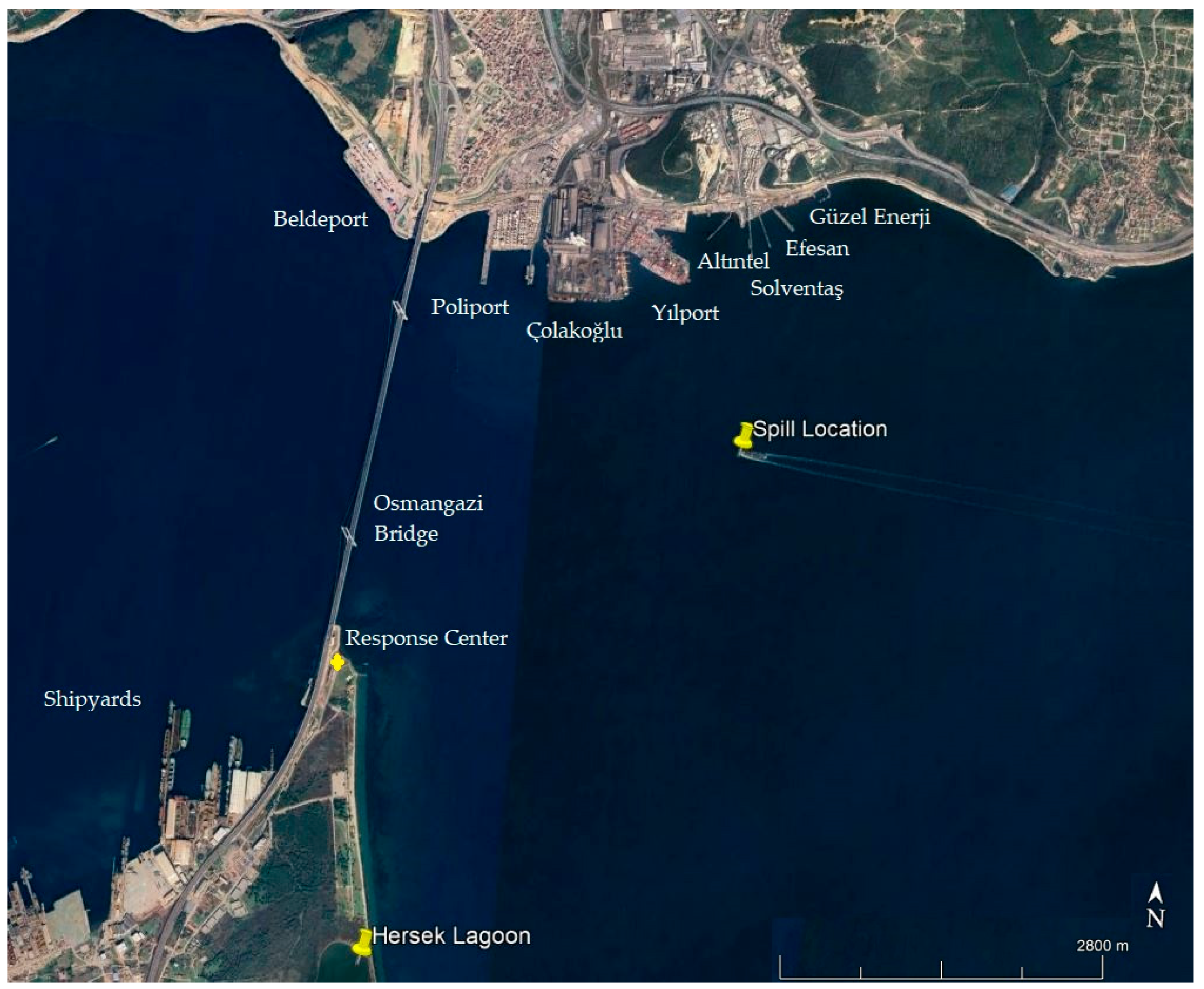
- Koseoglu, B.; Buber, M.; Toz, A.C. Optimum site selection for oil spill response center in the Marmara Sea using the AHP-TOPSIS method. Arch. Environ. Prot. 2018, 44, 38–49. [Google Scholar] [CrossRef]


| Crude Oil | API | Density (g/m3) at 17 °C | Viscosity, cSt at 17 °C | Wind |
|---|---|---|---|---|
| Kazakhstan Light Oil | 42.5 | 0.819 | 14.9 | NE 7 m/s |
| Evaporation (%) | Density (g/cm3) | Viscosity (cSt) | Spill Length (m) |
|---|---|---|---|
| 19.6 | 0.863 | 144 | 2000 |
| (a) | |||||||
| Year | Vessel Movements | Cargo Handled (Tons) | Maritime Accidents | Vessel Failures | Emergency Incidents | Rule Violation | Collision |
| 2023 | 43,145 | 90 | 12 | 33 | 66 | 126 | 2 |
| 2022 | 42,391 | 93 | 9 | 43 | 37 | 114 | 2 |
| 2021 | 42,167 | 85 | 4 | 36 | 53 | 143 | 0 |
| 2020 | 40,502 | 78 | 6 | 49 | 40 | 124 | 1 |
| 2019 | 39,150 | 75 | 6 | 43 | 27 | 120 | 3 |
| (b) | |||||||
| Year | Fire | Flooding | Grounding | Man Overboard | Sinking | Conflict | Accident Probability |
| 2023 | 1 | 1 | 1 | 1 | 1 | 5 | 2.78 × 10⁻⁴ |
| 2022 | 2 | 0 | 1 | 4 | 0 | 0 | 2.12 × 10⁻⁴ |
| 2021 | 0 | 1 | 1 | 0 | 0 | 2 | 9.49 × 10⁻⁴ |
| 2020 | 2 | 0 | 0 | 0 | 0 | 3 | 1.48 × 10⁻⁴ |
| 2019 | 0 | 0 | 0 | 0 | 0 | 3 | 1.53 × 10⁻⁴ |
Disclaimer/Publisher’s Note: The statements, opinions and data contained in all publications are solely those of the individual author(s) and contributor(s) and not of MDPI and/or the editor(s). MDPI and/or the editor(s) disclaim responsibility for any injury to people or property resulting from any ideas, methods, instructions or products referred to in the content. |
© 2025 by the authors. Licensee MDPI, Basel, Switzerland. This article is an open access article distributed under the terms and conditions of the Creative Commons Attribution (CC BY) license (https://creativecommons.org/licenses/by/4.0/).
Share and Cite
Balas, E.A.; Balas, C.E. Maritime Risk Assessment: A Cutting-Edge Hybrid Model Integrating Automated Machine Learning and Deep Learning with Hydrodynamic and Monte Carlo Simulations. J. Mar. Sci. Eng. 2025, 13, 939. https://doi.org/10.3390/jmse13050939
Balas EA, Balas CE. Maritime Risk Assessment: A Cutting-Edge Hybrid Model Integrating Automated Machine Learning and Deep Learning with Hydrodynamic and Monte Carlo Simulations. Journal of Marine Science and Engineering. 2025; 13(5):939. https://doi.org/10.3390/jmse13050939
Chicago/Turabian StyleBalas, Egemen Ander, and Can Elmar Balas. 2025. "Maritime Risk Assessment: A Cutting-Edge Hybrid Model Integrating Automated Machine Learning and Deep Learning with Hydrodynamic and Monte Carlo Simulations" Journal of Marine Science and Engineering 13, no. 5: 939. https://doi.org/10.3390/jmse13050939
APA StyleBalas, E. A., & Balas, C. E. (2025). Maritime Risk Assessment: A Cutting-Edge Hybrid Model Integrating Automated Machine Learning and Deep Learning with Hydrodynamic and Monte Carlo Simulations. Journal of Marine Science and Engineering, 13(5), 939. https://doi.org/10.3390/jmse13050939