1. Introduction
The rapid development of intelligent navigation technology and the widespread application of AISs (automatic identification systems) are driving ship navigation towards automation and unmanned operation [
1]. To achieve unmanned navigation [
2], ships need to compare their own trajectories with the routes stored in their system database and continuously adjust their own routes based on the similarity results. In terms of application, ship trajectory clustering methods have been widely used [
3]. However, during maritime navigation, vessels are subject to special conditions such as environmental factors and human influences, making traditional land-based trajectory similarity algorithms inadequate for meeting actual maritime needs. This necessitates the design of a measurement method for ship trajectory similarity that is tailored to the maritime field to meet practical requirements.
With the rapid development of computer technology and artificial intelligence, many scholars both domestically and internationally have proposed methods for measuring the trajectories of ships. This study takes a comparison between GPS-positioned trajectories and actual navigation tracks as an example to explore the requirements and methods for comparing trajectory similarity in the field of intelligent maritime navigation, particularly emphasizing the importance of similarity accuracy for intelligent navigation. Through analyzing existing similarity calculation processes and traditional similarity computation methods, we reveal their limitations in terms of their robustness and adaptability. To address these issues, this paper proposes a high-precision maritime vessel trajectory similarity assessment method. The method entails, first, a resampling approach that considers the accuracy of linear features to preprocess the given data, ensuring consistency in the data scale. Second, a shape feature extraction (shape feature extraction involves identifying and quantifying distinctive geometric or structural attributes of an object’s form to enable analysis, classification, or recognition in applications like computer vision and pattern recognition) and a transformation process for linear features are established, guaranteeing consistent feature extraction results across multi-scale and various scenarios and thereby enhancing the method’s robustness. Finally, a similarity evaluation criterion based on the “shape” feature extraction results is proposed, enabling quantitative comparison between updated and original data, and providing a scientific basis for currency assessment.
Trajectory similarity based on practical situations and existing algorithms: The algorithms that are traditionally used include the Hausdorff distance [
4], Frechet distance [
5], dynamic time warping (DTW) [
6], edit distance (ED) [
7], and longest common subsequence (LCSS) [
8] algorithms. However, traditional algorithms face significant issues in practical applications. For example, the DTW algorithm has a high computational complexity, making it unsuitable for long time series and difficult to apply in long-duration navigation. The ED and LCSS algorithms are quite robust in handling noise, but they are overly reliant on distance thresholds, which leads to poor measurement performance for trajectories with different sampling frequencies. The improved edit distance (IED) [
9] algorithm redefines the costs of insertion, deletion, and replacement operations for trajectory points based on actual spatial distances and specific matching rules. The fuzzy-based longest common subsequence (FLCSS) algorithm [
10] replaces the threshold of the LCSS algorithm with a fuzzy membership function and defines new matching methods for non-sampled points. Both methods reduce the dependence on distance thresholds and improve the robustness for trajectories with different sampling frequencies. Although sequence-based methods use dynamic programming to obtain a global optimal solution, they strictly follow the sequence order and rely only on the previous state for each calculation, which prevents them from discovering similar relationships between point pairs with significant differences in their sequence order. The Hausdorff distance and Frechet distance algorithms measure trajectory similarity solely based on the distance between a pair of key points, which cannot accurately capture the global characteristics of the trajectory.
Contemporary scholars have leveraged high-performance computing to enhance traditional algorithms, developing innovative approaches such as anchor point matching with distance correction for trajectory similarity measurement [
11], dynamic time warping (DTW) combined with trajectory point compression [
12], traffic flow-aware vessel trajectory similarity metrics [
13], and improved Fréchet distance-based methods for maritime trajectory similarity assessment [
14]. Trajectory similarity measures [
15]; review on trajectory similarity measures [
16]; review of trajectories similarity measures in mining algorithms [
17]; ship trajectory clustering based on trajectory resampling and enhanced BIRCH algorithm [
18]; a novel method for vessel trajectory clustering based on three-dimensional triangulation division algorithm [
19]; marine targets spatiotemporal trajectory similarity measurement method based on multidimensional features [
20]; clustering of maritime trajectories with ais features for context learning [
21]; charting the course of ship track prediction: a novel approach for maritime traffic analysis and enhanced situational awareness [
22]. These advancements exhibit substantial improvements over classical algorithms, offering enhanced “scale invariance” and “noise robustness”, and thereby enable the more accurate characterization of trajectory similarity across diverse spatial scales and under environmental noise. Additionally, they holistically integrate critical factors, including trajectory shape features, directional consistency between start and end points, and temporal intervals at trajectory endpoints, providing a multidimensional framework for robust similarity evaluation in complex maritime scenarios.
The aforementioned methods measure vessel trajectory similarity through spatial distance and shape analysis in their respective application domains. However, these algorithms fail to meet the “high-precision trajectory similarity comparison” requirements for intelligent maritime navigation, where discrepancies between satellite-acquired trajectories and database-stored historical routes often lead to hazardous navigational scenarios due to insufficient alignment accuracy. To address this challenge, this paper proposes a “high-precision maritime vessel trajectory similarity evaluation method” characterized by robust noise resistance and a registration-free framework. By quantifying similarity through shape feature extraction and multi-scale analysis, this method enables the precise, quantitative comparison of trajectory congruence without requiring spatial alignment pre-processing, thereby effectively mitigating operational risks in autonomous maritime navigation systems. Compared to the algorithms referenced in this study, the proposed method achieves three-decimal-place precision, demonstrating superior accuracy. The computational efficiency of the proposed method remains comparable to that of existing approaches, with execution times averaging approximately five seconds under equivalent experimental conditions. Additionally, the framework exhibits enhanced robustness, with significantly improved noise resistance capabilities compared to existing solutions.
Through the analysis of existing similarity computation workflows and traditional similarity calculation methods, this paper reveals the limitations of current algorithms: (1) current mainstream algorithms lack robustness and are susceptible to noise in propagated trajectories; (2) current mainstream algorithms exhibit low adaptability and cannot accommodate the diverse characteristics of ship trajectories across varying environments; (3) current mainstream algorithms lack sufficient precision to meet the high-accuracy requirements of maritime vessels. To address these issues, as referenced in the aforementioned literature, most authors primarily focus on innovating and integrating traditional algorithms to enhance their precision and robustness.
This paper is structured into the following sections:
Section 2 presents the algorithmic principle analysis;
Section 3 describes the algorithmic workflow;
Section 4 demonstrates the experimental procedures;
Section 5 provides the article’s conclusion.
2. Algorithm Principle Analysis
Existing line similarity discrimination methods exhibit limitations in threshold configuration and robustness. To enhance the algorithmic effectiveness of these methods, this paper proposes a line similarity evaluation method based on the shape feature extraction of linear features, addressing the requirement for line similarity computation in flight track comparative analysis. This approach carries out holistic evaluation through local segment matching, demonstrating strong robustness and reliability. The method first standardizes line features through resampling, the subsequently extracts shape characteristics via coordinate system transformation (coordinate system transformation converts spatial data between different reference frames (e.g., via translation, rotation, scaling) to align coordinates), and, finally, designs similarity metrics based on the Fréchet distance and DTW distance from feature extraction results, which collectively form a complete algorithmic framework. This section elaborates the methodological principles of this approach in detail.
2.1. Analysis of Resampling Accuracy Metrics
The current analysis methods of flight track data often rely on multi-source information such as GPS positioning and AIS data, which offer advantages including temporal currency, accessibility, and adaptability, and have been widely utilized in the production and updating of multi-scale vector spatial datasets. Drawing on existing deep learning methodologies, this study extracts historical trajectories from available vector data by leveraging prior information. However, factors such as waves, ocean currents, and weather conditions during navigation significantly influence the movements of ships, resulting in complex historical trajectories. Additionally, variations in vessel types and tonnage lead to inconsistent route selections during voyages, causing discrepancies in the scale and granularity of trajectory data. Consequently, directly extracted linear features often prove impractical due to exhibiting uneven node distribution, which introduces scale inconsistency during similarity comparisons and adversely affects evaluation outcomes.
To address this, this paper introduces a resampling procedure as a preprocessing step prior to the conducting of similarity evaluation, aiming to unify the scale discrepancies and uneven node distributions across linear features while controlling the node quantities to maintain the algorithm’s efficiency within manageable limits. Notably, although the resampling step exclusively serves to conduct the quantitative similarity assessment of linear features without altering the raw data, it inevitably raises concerns about potential inconsistencies between resampled and original linear features. To mitigate this, the precision thresholds for resampling are constrained based on the accuracy requirements across application scenarios, ensuring that the accuracy loss caused by resampling remains controllable. The accuracy assessment of the proposed resampling method is demonstrated in
Figure 1 below:
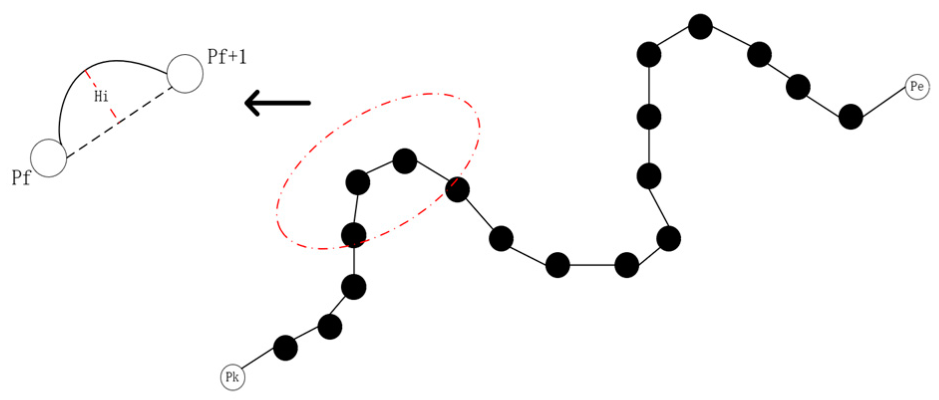
As illustrated, , and represent the start and end of a linear feature containing k nodes. If the shape of the entire linear feature is depicted solely through these nodes, it introduces “linear approximation” errors (replacing curves with straight lines). For example, in the intercepted segment that is shown, describing this portion using a straight line connecting node , results in a sagitta error —the precision loss distance caused by linear simplification.
To address how to set an appropriate step length for keeping the distance accuracy loss within acceptable limits in intelligent ship navigation scenarios, this study conducts a detailed analysis using comparison between GPS-derived trajectories and actual trajectories.
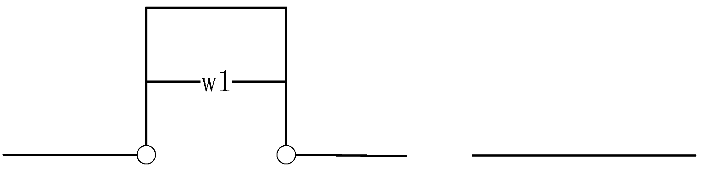
In marine applications, the CA-code single-frequency GPS navigators that are commonly used on ships exhibit a positioning accuracy of approximately 15 m. During actual navigation, scenarios may arise, as depicted in
Figure 2, where a vessel temporarily deviates from its original course to avoid an obstacle before returning. Here, w
1 represents the lateral displacement between the initial and adjusted courses. When w
1 falls below 15 m, the system automatically disregards the deviation, simplifying the trajectory into a straight line. To address this, this study establishes a maximum step length of 15 m, which inversely determines the number of resampling interpolation points. This approach ensures both scale consistency between linear features and maintains the accuracy of the resampled trajectory within standardized tolerances.
2.2. Reversibility Analysis of Linear Feature Shape Feature Extraction
In line similarity measurement, shape description is the most critical factor [
23]. Effective description should abstract the shape characteristics of linear features while maintaining invariance across scenarios and ensuring feature reversibility. Building on a comparative analysis of existing methods, this study develops a high-precision maritime vessel trajectory similarity assessment approach that fulfills these requirements. The current line similarity metrics include methods that compare shapes through feature extraction, yet those that rely solely on global characteristics inadequately capture the local details, while methods that emphasize local features fail to represent global patterns. As mentioned in the introduction, invariant moments have been proposed to document linear features, but they prove computationally intensive for complex shapes, struggle with multi-scale feature extraction, and cannot guarantee unique correspondence between the extracted features and original linear elements.
To address these challenges, this paper abstracts the concept of a “linear feature shape” by extracting inter-point relationships through coordinate system transformation, achieving effective feature extraction that remains robust across multi-scale scenarios. The methodology is as follows: First, the original linear feature
is transformed into the resampled feature
through preprocessing. Let
denote the Euclidean distance calculation, where
represents the number of nodes in
, and
indicates the
th-node. For each node
on
, compute its Euclidean distance to the feature’s starting point, then normalize this value by dividing it by the average distance.
In the formula, denotes the distance from the -th node of linear feature to the starting point (the first node of linear feature ).
Based on the obtained
, step (b) for linear feature extraction essentially entails a coordinate system transformation which sequentially converts each node in linear feature
into the following form:
In the formula, denotes the distance from node 0 to node in linear feature ; step b sequentially transforms all nodes of , which is illustrated here using node as an example, where its original coordinates are converted to .
In the aforementioned transformation process that takes place during feature extraction, the resampled node set
of the linear feature is reconstructed into a shape feature point set
. Notably, due to the resampling procedure, the Euclidean distance between consecutive nodes in this algorithm is equal and defined as
, as detailed below:
In the formula,
denotes the distance from node
to node
, and
represents the distance from node
to the starting point; these values are calculated as follows:
Thus, a linear feature model is established that is governed by fixed parameters. The step length is represented by
, the fixed distance is represented by
, and the fixed length is represented by
. The conceptual framework is illustrated in
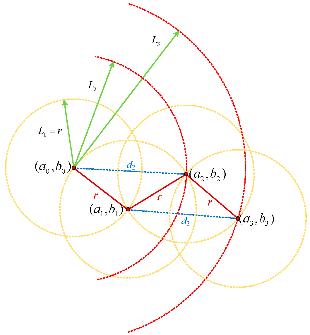
Figure 3 below:
As shown in the diagram, to reconstruct the original point set
from the resampled set
, the following geometric method is applied: Using the current node
as the center, a circle
is drawn with radius
. Simultaneously, another circle
is created with the starting point as the center and
as the radius. The intersection of these two circles determines the position of the next node
. Additionally, the distance between preceding and succeeding nodes of
f must satisfy the constraint
. Due to the algorithmic specificity in this study, the two circles are guaranteed to have at least one intersection point. When two intersections exist, the unique solution is determined by constraining
.
By solving the system of equations mentioned above, the coordinates of the intersection points
can be derived:
In the formula, the distance between circle centers is ; based on , the number of intersections between the two circles (one or two) is determined. The distance from an intersection point to the circle center and the distance from the intersection to the perpendicular bisector are then calculated, which ultimately derives the intersection coordinates . Consequently, at most two linear features can be reconstructed from . It follows that corresponds to a unique linear feature whose shape is fully preserved in the point set . Here, the coordinates present two possible cases, with the unique solution being determined by constraining . This demonstrates that, through transformation and extraction, is made to uniquely represent the shape of a linear feature.
2.3. Principle Analysis of Shape Feature Extraction for Linear Features
The preceding analysis demonstrates that this transformation and extraction process converts linear features into a point set that describes their shape characteristics and which corresponds to a unique linear feature shape. Building on this foundation, this section will analyze the inherent characteristics and significance embedded in the coordinates of the transformed point set, and discuss why this conversion can effectively represent the shape features of a linear feature.
As mentioned earlier, in the transformed point set
, each coordinate contains two elements:
denotes the distance from node
to node
, and
represents the distance from node
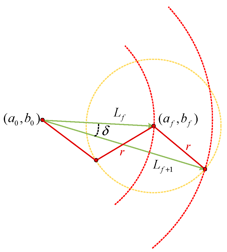
to the starting point. As illustrated in
Figure 4,
in the coordinates corresponds to the labeled
in the diagram. During preprocessing, the step length
is fixed. Given this fixed
and
, the angle
(in radians) between the current node (the circle center in the diagram) and its adjacent nodes can be calculated using the following formula:
In the equation above, it is evident that the coordinate value stores the feature of the angle β between the preceding and succeeding nodes at node , representing the bending characteristics of the linear feature. However, as shown in the diagram above, preserving only the angle β is insufficient to uniquely determine the corresponding point. This necessitates the use of the second coordinate value in the point set to impose additional constraints.
As shown in
Figure 5,
,
, and the step length
form a triangle, allowing the calculation of angle
(in radians) using the three known side lengths according to the law of cosines. The computational method is as follows:
This demonstrates that the transformed point set records two angles, and , which collectively characterize the linear feature.
As shown in
Figure 6, the transformed linear feature
encodes two angles,
and
, which enable the derivation of the coordinates of node
from node
, thereby constructing a point set to characterize the linear feature. Through coordinate system transformation, shape features are extracted. The proposed algorithm achieves robust performance in similarity matching by leveraging these shape features.
2.4. Evaluation and Analysis of Similarity Metrics
Through the above analysis, it is established that the proposed algorithm transforms original point sets into feature point sets that reflect the angles and of linear features via transformation and extraction. Simultaneously, during experimental validation, the authors discovered that retaining the most characteristic segments of linear features enables high matching accuracy through localized partial matching.
As introduced in
Section 2.3, this paper designs a linear similarity evaluation criterion that combined the averaged DTW distance and Fréchet distance after completing feature transformation and shape extraction. To eliminate the multi-scale effects of linear features, the criterion normalizes transformed coordinates, scaling linear features of varying lengths to a unified scale for comparison. The compared point sets are structured as
, where the two coordinate values reflect angles
and
, respectively, which collectively represents the shape characteristics of the entire linear feature. The similarity formula integrates two distance metrics: the DTW distance quantifies the global alignment quality between trajectories, while the Fréchet distance measures the maximum local shape deviation, with the two jointly ensuring comprehensive similarity assessment.
The DTW (dynamic time warping) distance employs a dynamic programming principle that enables non-linear temporal warping between sequences. This allows for the identification of optimal alignment points between two sequences even when they differ in length and shape. Specifically, DTW computes pairwise distances between all elements of one sequence and those of another, constructing a distance matrix. It then identifies a warping path through this matrix, via dynamic programming, that corresponds to the optimal alignment between sequences. During the path calculation, DTW enforces local constraints (e.g., limiting warping ranges) to ensure interpretable alignments. Owing to these characteristics, DTW has been widely applied in signal processing, speech recognition, and image analysis. The proposed algorithm leverages the DTW distance to quantify the local shape compatibility between linear features. As DTW’s computational methodology is extensively documented, it is not elaborated here.
The Fréchet distance is a method for comparing the similarity between two paths by considering the temporal progression and movement along their points. Specifically, the Fréchet distance is defined as the minimum distance required for two paths to traverse synchronously from their starting points at a uniform rate. When one path reaches its endpoint, the distance between the other path’s final position and its own endpoint defines their Fréchet distance. Leveraging this property, this paper incorporates the Fréchet distance between transformed linear features to quantify the maximum deviation in the shape characteristics of the original features, thereby capturing their structural dissimilarity.
By integrating these two distance metrics, the proposed algorithm’s similarity evaluation criterion comprehensively achieves registration-free similarity comparison between linear features. After transformation, the original spatial coordinates of two linear features are converted into shape characteristics, where the DTW distance between the transformed features reflects the local alignment of their original shapes, while the Fréchet distance captures the maximum deviation in their shape characteristics. Based on these two distances, the algorithm effectively quantifies the shape similarity between linear features, demonstrating higher accuracy compared to traditional similarity comparison methods without relying on manually set thresholds. The experimental results indicate that, even if one linear feature represents only a partial segment of another, retaining its characteristic portions still yields high similarity scores due to the preserved geometric invariants encoded in the transformed feature set
4. Experiments and Analysis
To evaluate the effectiveness and superiority of the proposed algorithm for line feature similarity assessment, this study implements the algorithm using the pytorch framework in a Python environment (version 3.13.1). The PIL library is utilized for visualizing and analyzing the experimental results. Three experimental designs are specifically formulated: (1) a reliability analysis experiment for the similarity evaluation metric, (2) an algorithm effectiveness experiment, and (3) a comparative experiment with existing methods. These experiments systematically validate the theoretical foundations proposed earlier from multiple perspectives. The experimental environment consists of an Intel(R) Core (TM) i9-12900H processor (2.50 GHz main frequency), 16 GB of RAM, and a GeForce GTX 3060 laptop GPU (The equipment was sourced Lenovo in Beijing, China).
4.1. Feasibility Experiment of Linear Feature Similarity Matching Method
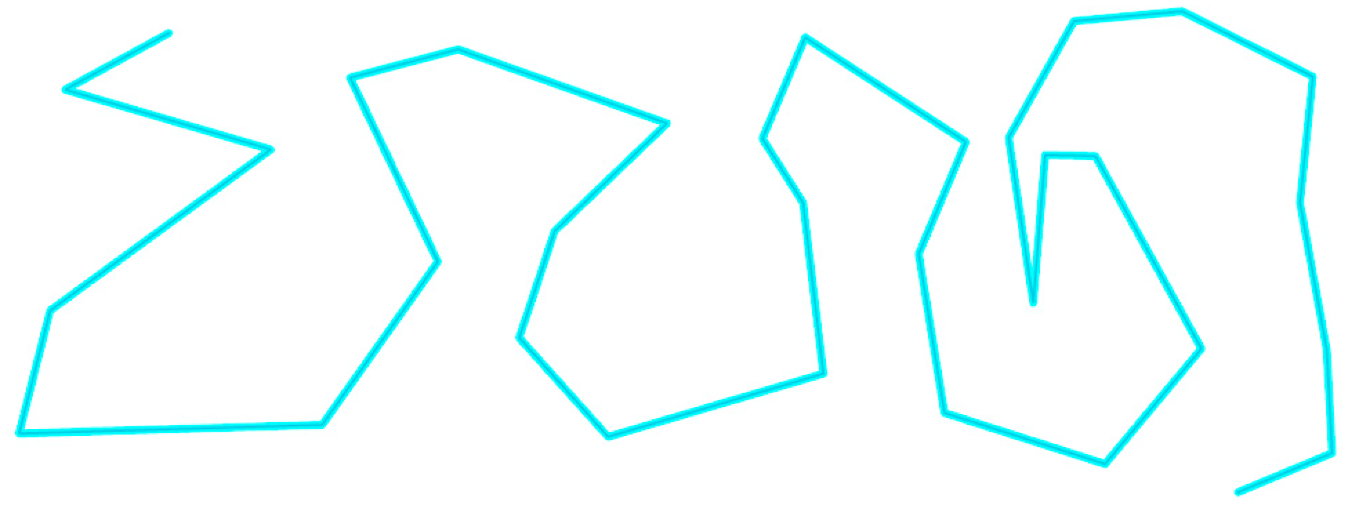
First, this experiment will verify the effectiveness of the proposed similarity evaluation metric. The experimental data employ a complex trajectory composed of 200 nodes, and self-comparisons are conducted for the data while cross-comparisons are conducted with other trajectories to validate the line similarity comparison method. The experimental data are shown in
Figure 8 and
Figure 9.
As shown in the figure, the selected experimental trajectory exhibits complex shapes and scaling characteristics, effectively demonstrating the validity of the proposed similarity evaluation metric. The specific experimental results of the similarity assessment for this complex trajectory are presented in
Table 1.
The intermediate process diagrams and final result diagrams of the line feature transformation conducted in this experiment are shown in
Table 2.
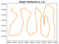
The comparative experimental results above demonstrate that the proposed line similarity evaluation method achieves a 100% similarity score when the test trajectory is compared against itself, and 0% similarity when it is compared against trajectories with significantly dissimilar shapes. This validates the methodological feasibility of the proposed line similarity comparison approach.
4.2. Effectiveness Experiment of the Linear Feature Similarity Quantitative Evaluation Method
4.2.1. Multi-Scale Linear Feature Similarity Matching Experiment
The first experiment involves multi-scale trajectory similarity matching. To validate the effectiveness of the proposed line similarity quantification method, a multi-scale similarity matching test was conducted on a relatively complex trajectory. The experimental dataset used in the test region is illustrated in the figure below (highlighted section represents the adopted linear feature).
As shown in
Figure 10, the experiment utilizes three distinct linear features with similar shapes from the same region. This validation test confirms the effectiveness of the proposed algorithm. The experimental analysis results from pairwise comparisons of these three linear features are presented in the table below.
According to
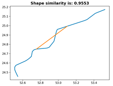
Table 3, the results show that the self-similarity evaluation metric for the same linear feature achieves 100%, meeting the required criteria. Despite significant morphological and characteristic differences between Line3 and Line1/Line2, their similarity scores reach 96.00% and 97.05%, respectively. Line1 and Line2, which share similar features and align in key bending sections, attain a high similarity score of 99.71%, which is consistent with expectations. To visually demonstrate the DTW and Fréchet distance calculations between the transformed linear features, intermediate process diagrams and result diagrams from the experiment are provided.
From
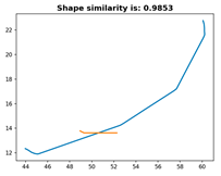
Table 4, it can be seen that the proposed algorithm demonstrates robust similarity computation capabilities under multi-scale conditions, effectively matching partial segments to the entire trajectory. Notably, in Experiment 2_6, Line4 achieved a similarity score of 99.57% despite retaining only two points, which is attributed to the preservation of the most “characteristic” segment of the trajectory. In Experiments 2_4 and 2_5, the comparisons between Line2 and Line3/Line4 also yielded similarity scores exceeding 95%, which validates our hypothesis and confirms the algorithm’s capability of computing similarity under multi-scale conditions. These experiments demonstrate that the proposed algorithm can effectively compare linear features across different scales with strong robustness.
4.2.2. Overall Effectiveness Experiment of Local Matching
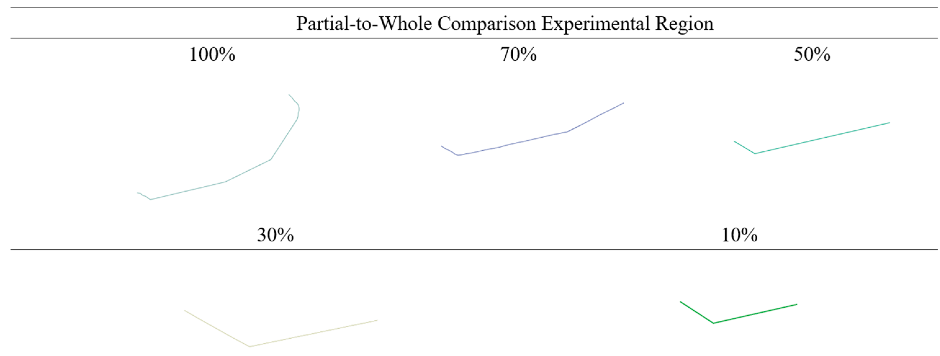
To validate the claim that retaining partial characteristic regions of linear features can maintain high similarity metrics with the original features, this paper conducts a partial–whole comparison experiment. The experimental region uses a trajectory segmented into 70%, 50%, 30%, and 10% portions of the original line feature. The experimental area is illustrated in the figure below.
As shown in
Figure 11, the experimental linear features are different segments of the same original feature. Through this validity test, the effectiveness of the proposed algorithm in matching local regions to the entire feature can be evaluated. The experimental results are presented in the following table.
From
Table 5, it can be seen that the similarity evaluation metric for the same linear feature is 100%, meeting the requirements. As the linear feature is progressively truncated, the similarity decreases. Notably, Experiment 3_4 retains a similarity of 98.53%, with only 30% of the original feature having been preserved. This is attributed to the model retaining the most “characteristic” portion of the linear feature. To validate the reliability of this hypothesis, Experiment 3_5 was conducted. Under the same 10% truncation of the original feature, Experiment 3_5 captured a varying “characteristic” segment. As hypothesized, Experiment 3_5 achieved a high similarity of 99.50% with only 10% of the feature having been retained, which further supports the algorithm’s capability of matching local segments to the entire feature. To visually demonstrate the process of calculating the DTW and Fréchet distances between transformed feature sets and deriving the similarity metric, intermediate transformation steps and results are presented in
Table 6.
As shown in
Table 6, the proposed algorithm effectively matches partial segments to the entire linear feature, achieving higher similarity accuracy particularly when the “characteristic” portions of the linear feature are preserved.
4.3. Limitations of the Study
The algorithm proposed in this paper still has certain potential limitations when facing real-world conditions. Below, we will analyze these issues and propose future directions of improvement.
Currently, the algorithm primarily relies on GPS satellite data. However, the positioning accuracy of GPS is inherently limited, and maritime vessel data can be obtained through various methods, such as radar and AIS, which leads to significant limitations when applying the proposed algorithm to such scenarios. Additionally, the algorithm is constructed based on latitude-longitude coordinates. When processing data without such coordinates, it cannot extract the information required for similarity analysis. The computation time also requires improvement—the current algorithm takes approximately five seconds, which is acceptable on high-performance computers but becomes significantly longer on typical vessel systems with lower computational capabilities, hindering the comparison of similarities in real-time.
In the future, we will optimize the algorithm to accommodate multiple data sources, enhancing its applicability. Further improvements will focus on streamlining the algorithm’s structure, reducing redundant computations, accelerating its processing speed, and lowering its hardware requirements to meet the needs of most maritime vessels.
5. Conclusions
This study takes a comparison between GPS-positioned trajectories and actual navigation tracks as an example to explore the requirements and methods for comparing trajectory similarities in the field of intelligent maritime navigation, particularly emphasizing the importance of similarity accuracy for intelligent navigation. Through analyzing existing similarity calculation processes and traditional similarity computation methods, we reveal their limitations in robustness and adaptability. To address these issues, this paper proposes a high-precision maritime vessel trajectory similarity assessment method. The method first designs a resampling approach that considers the accuracy of linear features to preprocess the data, ensuring consistency in the scale of the data. Second, it establishes a shape feature extraction and transformation process for linear features, guaranteeing consistent feature extraction results across multi-scale and various scenarios and thereby enhancing the method’s robustness. Finally, it proposes a similarity evaluation criterion based on “shape” feature extraction results, enabling quantitative comparison between updated and original data, and providing a scientific basis for currency assessment.
This research provides effective technical support for advancing intelligent maritime navigation and opens new perspectives regarding and methods for the similarity analysis of other maritime vessel trajectories. Future studies could explore the applicability of this method in more application scenarios, such as urban planning and environmental monitoring. Integrating machine learning and deep learning technologies holds potential to further improve the accuracy and automation level of similarity evaluation, promoting the profound development of intelligent maritime navigation technology.


